Quasiperiodic Motion for the Pentagram Map

1 Introduction and main results

The pentagram map, $T$, is a natural operation one can perform on polygons. See [S1], [S2] and [OST] for the history of this map and additional references. Though this map can be defined for an essentially arbitrary polygon over an essentially arbitrary field, it is easiest to describe the map for convex polygons contained in $\mbox{\boldmath{$R$}}^{2}$. Given such an $n$-gon $P$, the corresponding $n$-gon $T(P)$ is the convex hull of the intersection points of consecutive shortest diagonals of $P$. Figure 1 shows two examples.

Figure 1: The pentagram map defined on a pentagon and a hexagon

Thinking of $\mbox{\boldmath{$R$}}^{2}$ as a natural subset of the projective plane $\mbox{\boldmath{$R$}}\mbox{\boldmath{$P$}}^{2}$, we observe that the pentagram map commutes with projective transformations. That is, $\phi(T(P))=T(\phi(P))$, for any $\phi\in\mathrm{PGL}(3,\mbox{\boldmath{$R$}})$. Let ${\cal C\/}_{n}$ be the space of convex $n$-gons modulo projective transformations. The pentagram map induces a self-diffeomorphism $T:{\cal C\/}_{n}\to{\cal C\/}_{n}$.

$T$ is the identity map on ${\cal C\/}_{5}$ and an involution on ${\cal C\/}_{6}$, cf. [S1]. For $n\geq 7$, the map $T$ exhibits quasi-periodic properties. Experimentally, the orbits of $T$ on ${\cal C\/}_{n}$ exhibit the kind of quasiperiodic motion associated to a completely integrable system. More precisely, $T$ preserves a certain foliation of ${\cal C\/}_{n}$ by roughly half-dimensional tori, and the action of $T$ on each torus is conjugate to a rotation. A conjecture [S2] that $T$ is completely integrable on ${\cal C\/}_{n}$ is still open. However, our recent paper [OST] very nearly proves this result.

Rather than work directly with ${\cal C\/}_{n}$, we work with a slightly larger space. A twisted $n$-gon is a map $\phi:\mbox{\boldmath{$Z$}}\to\mbox{\boldmath{$R$}}\mbox{\boldmath{$P$}}^{2}$ such that

$$\phi(n+k)=M\circ\phi(k);\hskip 40.0pt\forall k\in\mbox{\boldmath{$Z$}},$$

for some fixed element $M\in\mathrm{PGL}(3,\mbox{\boldmath{$R$}})$ called the monodromy. We let $v_{i}=\phi(i)$ and assume that $v_{i-1},v_{i},v_{i+1}$ are in general position for all $i$. We denote by ${\cal P\/}_{n}$ the space of twisted $n$-gons modulo projective equivalence. We show that the pentagram map $T:{\cal P\/}_{n}\to{\cal P\/}_{n}$ is completely integrable in the classical sense of Arnold–Liouville. We give an explicit construction of a $T$-invariant Poisson structure and complete list of Poisson-commuting invariants (or integrals) for the map. This is the algebraic part of our theory.

The space ${\cal C\/}_{n}$ is naturally a subspace of ${\cal P\/}_{n}$, and our algebraic results say something (but not quite enough) about the action of the pentagram map on ${\cal C\/}_{n}$. There are still some details about how the Poisson structure and the invariants restrict to ${\cal C\/}_{n}$ that we have yet to work out. To get a crisp geometric result, we work with a related space, which we describe next.

We say that a twisted $n$-polygon is universally convex if the map $\phi$ is such that $\phi(\mbox{\boldmath{$Z$}})\subset\mbox{\boldmath{$R$}}^{2}\subset\mbox{\boldmath{$R$}}\mbox{\boldmath{$P$}}^{2}$ is convex and contained in the positive quadrant. We also require that the monodromy $M:\mbox{\boldmath{$R$}}^{2}\to\mbox{\boldmath{$R$}}^{2}$ is a linear transformation having the form

$$M=\left[\begin{matrix}a&0\cr 0&b\end{matrix}\right];\hskip 40.0pta<1<b.$$ (1)

The image of $\phi$ looks somewhat like a “polygonal hyperbola”. We say that two universally convex twisted $n$-gons $\phi_{1}$ and $\phi_{2}$ are equivalent if there is a positive diagonal matrix $\mu$ such that $\mu\circ\phi_{1}=\phi_{2}$. Let ${\cal U\/}_{n}$ denote the space of universally convex twisted $n$-gons modulo equivalence. It turns out that ${\cal U\/}_{n}$ is a pentagram-invariant and open subset of ${\cal P\/}_{n}$. Here is our main geometric result.

Theorem 1.1

Almost every pont of ${\cal U\/}_{n}$ lies on a smooth torus that has a $T$-invariant affine structure. Hence, the orbit of almost every universally convex $n$-gon undergoes quasi-periodic motion under the pentagram map.

2 Sketch of the Proof

In this section we will sketch the main ideas in the proof of Theorem 1.1. We refer the reader to [OST] for more results and details.

2.1 Coordinates

Recall that the cross ratio of $4$ collinear points in $\mbox{\boldmath{$R$}}\mbox{\boldmath{$P$}}^{2}$ is given by

$$[t_{1},t_{2},t_{3},t_{4}]=\frac{(t_{1}-t_{2})\,(t_{3}-t_{4})}{(t_{1}-t_{3})\,(t_{2}-t_{4})},$$

where $t$ is (an arbitrary) affine parameter. We use the cross ratio to construct coordinates on the space of twisted polygons. We associate to every vertex $v_{i}$ two numbers:

$$\begin{array}[]{rcl}x_{i}&=&\displaystyle\left[v_{i-2},\,v_{i-1},\,\left((v_{i-2},v_{i-1})\cap(v_{i},v_{i+1})\right),\,\left((v_{i-2},v_{i-1})\cap(v_{i+1},v_{i+2})\right)\right]\\[10.0pt] y_{i}&=&\displaystyle[\left((v_{i-2},v_{i-1})\cap(v_{i+1},v_{i+2})\right),\,\left((v_{i-1},v_{i})\cap(v_{i+1},v_{i+2})\right),\,v_{i+1},\,v_{i+2}]\end{array}$$

called the left and right corner cross-ratios, see Figure 2. We call our coordinates the corner invariants.

Figure 2: Points involved in the definition of the invariants

This construction is invariant under projective transformations, and thus gives us coordinates on the space ${\cal P\/}_{n}$. At generic points, ${\cal P\/}_{n}$ is locally diffeomorphic to $\mbox{\boldmath{$R$}}^{2n}$.

We will work with generic elements of ${\cal P\/}_{n}$, so that all constructions are well-defined. Let $\phi^{*}=T(\phi)$ be the image of $\phi$ under the pentagram map. We choose the labelling scheme shown in Figure 3. The black dots represent $\phi$ and the white ones represent $\phi^{*}$.

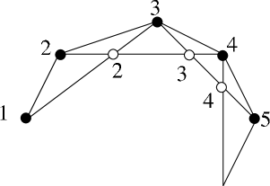
Figure 3: The labelling scheme

Now we describe the pentagram map in coordinates.

$$T^{*}x_{i}=x_{i}\,\frac{1-x_{i-1}\,y_{i-1}}{1-x_{i+1}\,y_{i+1}},\qquad T^{*}y_{i}=y_{i+1}\,\frac{1-x_{i+2}\,y_{i+2}}{1-x_{i}\,y_{i}},$$ (2)

Equation 2 has two immediate corollaroes. First, there is an interesting scaling symmetry of the pentagram map. We have a rescaling operation given by the expression

$$R_{t}:\hskip 10.0pt(x_{1},y_{1},...,x_{n},y_{n})\to(tx_{1},t^{-1}y_{1},...,tx_{n},t^{-1}y_{n}).$$ (3)

Corollary 2.1

The pentagram map commutes with the rescaling operation.

Second, the formula exhibits rather quickly some invariants of the pentagram map. For all $n$, define

$$O_{n}=\prod_{i=1}^{n}x_{i};\hskip 30.0ptE_{n}=\prod_{i=1}^{n}y_{i}$$ (4)

When $n$ is even, define also

$$O_{n/2}=\prod_{i\ {\rm even\/}}x_{i}+\prod_{i\ {\rm odd\/}}x_{i}.\hskip 20.0ptE_{n/2}=\prod_{i\ {\rm even\/}}y_{i}+\prod_{i\ {\rm odd\/}}y_{i}.$$ (5)

The products in this last equation run from $1$ to $n$.

Corollary 2.2

The functions $O_{n}$ and $E_{n}$ are invariant under the pentagram map. When $n$ is even, the functions $O_{n/2}$ and $E_{n/2}$ are also invariant under the pentagram map.

2.2 The Monodromy Invariants

In this section we describe the invariants of the pentagram map. We call them the monodromy invariants. As above, let $\phi$ be a twisted $n$-gon with invariants $x_{1},y_{1},...$. Let $M$ be the monodromy of $\phi$. We lift $M$ to an element of $\mathrm{GL}_{3}(\mbox{\boldmath{$R$}})$. By slightly abusing notation, we also denote this matrix by $M$. The two quantities

$$\Omega_{1}=\frac{{\rm trace\/}^{3}(M)}{{\rm det\/}(M)};\hskip 40.0pt\Omega_{2}=\frac{{\rm trace\/}^{3}(M^{-1})}{{\rm det\/}(M^{-1})};$$

are only dependent on the conjugacy class of $M$.

We define

$$\widetilde{\Omega}_{1}=O_{n}^{2}E_{n}\Omega_{1};\hskip 30.0pt\widetilde{\Omega}_{2}=O_{n}E_{n}^{2}\Omega_{2}.$$

In [S3] (and again in [OST]) it is shown that $\widetilde{\Omega}_{1}$ and $\widetilde{\Omega}_{2}$ are polynomials in the corner invariants. Since the pentagram map preserves the monodromy, and $O_{n}$ and $E_{n}$ are invariants, the two functions $\widetilde{\Omega}_{1}$ and $\widetilde{\Omega}_{2}$ are also invariants.

We say that a polynomial in the corner invariants has weight $k$ if

$$R_{t}^{*}(P)=t^{k}P.$$

here $R_{t}^{*}$ denotes the natural operation on polynomials defined by the rescaling operation above. For instance, $O_{n}$ has weight $n$ and $E_{n}$ has weight $-n$. In [S3] it shown that

$$\widetilde{\Omega}_{1}=\sum_{k=1}^{[n/2]}O_{k};\hskip 30.0pt\widetilde{\Omega}_{2}=\sum_{k=1}^{[n/2]}E_{k}$$

where $O_{k}$ has weight $k$ and $E_{k}$ has weight $-k$. Since the pentagram map commutes with the rescaling operation and preserves $\widetilde{\Omega}_{1}$ and $\widetilde{\Omega}_{2}$, it also preserves their “weighted homogeneous parts”. That is, the functions $O_{1},E_{1},\allowbreak O_{2},E_{2},...$ are also invariants of the pentagram map. These are the monodromy invariants. They are all nontrivial polynomials. In [S3] it is shown that the monodromy invariants are algebraically independent.

The explicit formulas for the monodromy invariants was obtained in [S3]. Introduce the monomials

$$X_{i}:=x_{i}\,y_{i}\,x_{i+1}.$$

1. We call two monomials $X_{i}$ and $X_{j}$ consecutive if $j\in\left\{i-2,\,i-1,\,i,\,i+1,\,i+2\right\};$

2. we call $X_{i}$ and $x_{j}$ consecutive if $j\in\left\{i-1,\,i,\,i+1,\,i+2\right\};$

3. we call $x_{i}$ and $x_{i+1}$ consecutive.

Let $O(X,x)$ be a monomial obtained by the product of the monomials $X_{i}$ and $x_{j}$, i.e.,

$$O=X_{i_{1}}\cdots{}X_{i_{s}}\,x_{j_{1}}\cdots{}x_{j_{t}}.$$

Such a monomial is called admissible if no two of the indices are consecutive. For every admissible monomial, we define the weight $|O|=s+t$ and the sign $\mathrm{sign}(O)=(-1)^{t}$. One then has

$$O_{k}=\sum_{|O|=k}\mathrm{sign}(O)\,O;\hskip 30.0ptk\in\left\{1,2,\ldots,\left[\frac{n}{2}\right]\right\}.$$

The same formula works for $E_{k}$, if we make all the same definitions with $x$ and $y$ interchanged.

2.3 The Poisson Bracket

In [OST] we introduce the Poisson bracket on $C^{\infty}({\cal P\/}_{n})$. For the coordinate functions we set

$$\{x_{i},x_{i\pm 1}\}=\mp{}x_{i}\,x_{i+1},\qquad\{y_{i},y_{i\pm 1}\}=\pm{}y_{i}\,y_{i+1}$$ (6)

and all other brackets vanish. Once we have the definition on the coordinate functions, we use linearity and the Liebniz rule to extend to all rational functions. An easy exercise shows that the Jacobi identity holds.

Recall the standard notions of Poisson geometry. Two functions $f$ and $g$ are said to Poisson commute if $\{f,g\}=0$. A function $f$ is said to be a Casimir (relative to the Poisson structure) if $f$ Poisson commutes with all other functions. The corank of a Poisson bracket on a smooth manifold is the codimension of the generic symplectic leaves. These symplectic leaves can be locally described as levels $f_{i}=\mathrm{const}$ of the Casimir functions.

The main lemmas of [OST] concerning our Poisson bracket are as follows.

1. The Poisson bracket (6) is invariant with respect to the Pentagram map.

2. The monodromy invariants Poisson commute.

3. The invariants in Equations (4) and (in the even case) (5) are Casimirs.

4. The Poisson bracket has corank $2$ if $n$ if odd and corank $4$ if $n$ is even.

We now consider the case when $n$ is odd. The even case is similar. On the space ${\cal P\/}_{n}$ we have a generically defined and $T$-invariant Poisson bracked that is invariant under the pentagram map. This bracket has co-rank $2$, and the generic level set of the Casimir functions has dimension $4[n/2]=2n-2$. On the other hand, after we exclude the two Casimirs, we have $2[n/2]=n-1$ algebraically independent invariants that Poisson commute with each other. This gives us the classical Liouville-Arnold complete integrability.

2.4 The End of the Proof

Now we specialize our algebraic result to the space ${\cal U\/}_{n}$ of universally convex twisted $n$-gons. We check that ${\cal U\/}_{n}$ is an open and invariant subset of ${\cal P\/}_{n}$. The invariance is pretty clear. The openness result derives from $3$ facts.

1. Local convexity is stable under perturbation.

2. The linear transformations in Equation 1 extend to projective transformations whose type is stable under small perturbations.

3. A locally convex twisted polygon that has the kind of hyperbolic monodromy given in Equation 1 is actually globally convex.

As a final ingredient in our proof, we show that the leaves of ${\cal U\/}_{n}$, namely the level sets of the monodromy invariants, are compact. We don’t need to consider all the invariants; we just show in a direct way that the level sets of $E_{n}$ and $O_{n}$ together are compact.

The rest of the proof is the usual application of Sard’s theorem and the definition of integrability. We explain the main idea in the odd case. The space ${\cal U\/}_{n}$ is locally diffeomorphic to $\mbox{\boldmath{$R$}}^{2n}$, and foliated by leaves which generically are smooth compact symplectic manifolds of dimension $2n-2$. A generic point in a generic leaf lies on an $(n-1)$ dimensional smooth compact manifold, the level set of our monodromy invariants. On a generic leaf, the symplectic gradients of the monodromy functions are linearly independent at each point of the leaf.

The $n-1$ symplectic gradients of the monodrony invariants give a natural basis of the tangent space at each point of our generic leaf. This basis is invariant under the pentagram map, and also under the Hamiltonian flows determined by the invariants. This gives us a smooth compact $n-1$ manifold, admitting $n-1$ commuting flows that preserve a natural affine structure. From here, we see that the leaf must be a torus. The pentagram map preserves the canonical basis of the torus at each point, and hence acts as a translation. This is the quasi-periodic motion of Theorem 1.1.

3 Pentagram map as a discrete Boussinesq equation

Remarkably enough, the continuous limit of the pentagram map is precisely the classical Boussinesq equation which is one of the best known infinite-dimensional integrable systems. This was already noticed in [S2] and efficiently used in [OST]. Discretization of the Boussinesq equation is an interesting and wel-studied subject, see [TN] and references therein. However, known versions of discrete Boussinesq equation lack geometric interpretation.

For technical reasons we assume throughout this section that $n\not=3\,m$.

3.1 Difference equations and global coordinates

It is a powerful general idea of projective differential geometry to represent geometrical objects in an algebraic way. It turns out that the space of twisted $n$-gons is naturally isomorphic to a space of difference equations.

To obtain a difference equation from a twisted polygon, lift its vertices $v_{i}$ to points $V_{i}\in\mbox{\boldmath{$R$}}^{3}$ so that $\det(V_{i},V_{i+1},V_{i+2})=1$. Then

$$V_{i+3}=a_{i}\,V_{i+2}+b_{i}\,V_{i+1}+V_{i}$$ (7)

where $a_{i},b_{i}$ are $n$-periodic sequences of real numbers. Conversely, given two arbitrary $n$-periodic sequences $(a_{i}),\,(b_{i})$, the difference equation (7) determines a projective equivalence class of a twisted polygon. This provides a global coordinate system $(a_{i},\,b_{i})$ on the space of twisted $n$-gons.

Corollary 3.1

If $n$ is not divisible by 3 then the space ${\cal P\/}_{n}$ is isomorphic to $\mbox{\boldmath{$R$}}^{2n}$.

When $n$ is divisible by $3$, the topology of the space is trickier.

The relation between coordinates is as follows:

$$x_{i}=\frac{a_{i-2}}{b_{i-2}\,b_{i-1}},\quad y_{i}=-\frac{b_{i-1}}{a_{i-2}\,a_{i-1}}.$$

The explicit formula for the pentagram map and the Poisson structure in the coordinates $(a_{i},\,b_{i})$ is more complicated that (2). Assume $n=3m+1$ or $n=3m+2$. Then

$$T^{*}a_{i}=a_{i+2}\,\prod_{k=1}^{m}\frac{1+a_{i+3k+2}\,b_{i+3k+1}}{1+a_{i-3k+2}\,b_{i-3k+1}},\qquad T^{*}b_{i}=b_{i-1}\,\prod_{k=1}^{m}\frac{1+a_{i-3k-2}\,b_{i-3k-1}}{1+a_{i+3k-2}\,b_{i+3k-1}};$$ (8)

the Poisson bracket (6) is defined on the coordinate functions as follows:

$$\begin{array}[]{rcl}\{a_{i},a_{j}\}&=&\displaystyle\sum_{k=1}^{m}\left(\delta_{i,j+3k}-\delta_{i,j-3k}\right)a_{i}\,a_{j},\\[16.0pt] \{a_{i},b_{j}\}&=&0,\\[6.0pt] \{b_{i},b_{j}\}&=&\displaystyle\sum_{k=1}^{m}\left(\delta_{i,j-3k}-\delta_{i,j+3k}\right)b_{i}\,b_{j}.\end{array}$$ (9)

The monodromy invariants also have a nice combinatorial description in the $(a,b)$-coordinates, cf. [OST].

3.2 The continuous limit

We understand the $n\to\infty$ continuous limit of a twisted $n$-gon as a smooth parametrized curve $\gamma:\mbox{\boldmath{$R$}}\to\mbox{\boldmath{$R$}}\mbox{\boldmath{$P$}}^{2}$ with monodromy:

$$\gamma(x+1)=M(\gamma(x)),$$

for all $x\in\mbox{\boldmath{$R$}}$, where $M\in\mathrm{PGL}(3,\mbox{\boldmath{$R$}})$ is fixed. The assumption that every three consequtive points are in general position corresponds to the assumption that the vectors $\gamma^{\prime}(x)$ and $\gamma^{\prime\prime}(x)$ are linearly independent for all $x\in\mbox{\boldmath{$R$}}$. A curve $\gamma$ satisfying these conditions is usually called non-degenerate. As in the discrete case, we consider classes of projectively equivalent curves.

The space of non-degenerate curves is very well known in classical projective differential geometry. There exists a one-to-one correspondence between this space and the space of linear differential operators on $R$:

$$A=\left(\frac{d}{dx}\right)^{3}+\frac{1}{2}\left(u(x)\,\frac{d}{dx}+\frac{d}{dx}\,u(x)\right)+w(x),$$

where $u$ and $w$ are smooth periodic functions.

We are looking for a continuous analog of the map $T$. The construction is as follows. Given a non-degenerate curve $\gamma(x)$, at each point $x$ we draw the chord $\left(\gamma(x-\varepsilon),\gamma(x+\varepsilon)\right)$ and obtain a new curve, $\gamma_{\varepsilon}(x)$, as the envelop of these chords, see Figure 4. Let $u_{\varepsilon}$ and $w_{\varepsilon}$ be the respective periodic functions. It turns out that

$$u_{\varepsilon}=u+\varepsilon^{2}\widetilde{u}+(\varepsilon^{3}),\quad w_{\varepsilon}=w+\varepsilon^{2}\widetilde{w}+(\varepsilon^{3}),$$

giving the curve flow: $\dot{u}=\widetilde{u},\ \dot{w}=\widetilde{w}$. We show that

$$\dot{u}=w^{\prime},\quad\displaystyle\dot{w}=\displaystyle-\frac{u\,u^{\prime}}{3}-\frac{u^{\prime\prime\prime}}{12},$$

or

$$\ddot{u}+\frac{\left(u^{2}\right)^{\prime\prime}}{6}+\frac{u^{(IV)}}{12}=0,$$

which is nothing else but the classical Boussinesq equation.

Figure 4: Evolution of a non-degenerate curve

Consider the space of functionals of the form

$$H(u,w)=\int_{S^{1}}h(u,u^{\prime},\ldots,w,w^{\prime},\ldots)\,dx,$$

where $h$ is a polynomial. The first Poisson bracket on the above space of functionals is defined by

$$\{G,H\}=\int_{S^{1}}\left(\delta_{u}G\left(\delta_{w}H\right)^{\prime}+\delta_{w}G\left(\delta_{u}H\right)^{\prime}\right)dx,$$ (10)

where $\delta_{u}H$ and $\delta_{w}H$ are the standard variational derivatives. The Poisson bracket (9) is a discrete version of the bracket (10).

Concluding remarks

As it happens, this work provides more open problems than established theorems. Let us mention here the problems that we consider most important.

1. Is there there another, second $T$-invariant Poisson bracket, compatible with the above described one? A positive answer would allow one to apply to the pentagram map the powerful bi-Hamiltonian techniques. It could also help to answer the next question.

2. Is the restriction of the pentagram map to the space ${\cal C\/}_{n}$ of closed polygons integrable?

3. Perhaps the most exciting open problem is to understand the relation of the pentagram map to cluster algebras. It is known that the space ${\cal P\/}_{n}$ is a cluster manifold; besides, our Poisson bracket has a striking similarity with the canonical Poisson bracket on cluster manifolds [GSV], see [OST] for a more detailed discussion.

Acknowledgments. R. S. and S. T. were partially supported by NSF grants, DMS-0604426 and DMS-0555803, respectively. V. O. and S. T. are grateful to the Research in Teams program at BIRS for its hospitality.

4 References

[A] V. I. Arnold, Mathematical Methods of Classical Mechanics, Graduate Texts in Mathematics 60, Springer-Verlag, New York, 1989.

[GSV] M. Gekhtman, M. Shapiro, A. Vainshtein, Cluster algebras and Poisson geometry, Mosc. Math. J. 3 (2003), 899–934.

[OST] V. Ovsienko, S. Tabachnikov, R. Schwartz, The Pentagram Map: A Discrete Integrable System, submitted (2008).

[S1] R. Schwartz, The Pentagram Map, Experimental Math. 1 (1992), 71–81.

[S2] R. Schwartz, Discrete Monodomy, Pentagrams, and the Method of Condensation J. Fixed Point Theory Appl. 3 (2008), 379–409.

[TN] A. Tongas, F. Nijhoff, The Boussinesq integrable system: compatible lattice and continuum structures, Glasg. Math. J. 47 (2005), 205–219.

Valentin Ovsienko: CNRS, Institut Camille Jordan, Université Lyon 1, Villeurbanne Cedex 69622, France, ovsienko@math.univ-lyon1.fr

Serge Tabachnikov: Department of Mathematics, Pennsylvania State University, University Park, PA 16802, USA, tabachni@math.psu.edu

Richard Evan Schwartz: Department of Mathematics, Brown University, Providence, RI 02912, USA, res@math.brown.edu