Dynamics of a three-dimensional inextensible chain

Abstract

In the first part of this work the classical and statistical aspects of the dynamics of an inextensible chain in three dimensions are investigated. In the second part the special case of a chain admitting only fixed angles with respect to the $z-$axis is studied using a path integral approach. It is shown that it is possible to reduce this problem to a two-dimensional case, in a way which is similar to the reduction of the statistical mechanics of a directed polymer to the random walk of a two-dimensional particle.

05.40.-a, 11.10.Lm, 61.25.H-

1 Introduction

In this report we investigate the dynamics of an inextensible three-dimensional chain fluctuating in some medium at fixed temperature $T$. The chain is considered as the continuous limit of a freely jointed chain, which consists of a set of $N-1$ rigid links of length $a$ and $N$ beads of mass $m$ attached at the joints between two consecutive segments. The formulation of the dynamics of a chain with rigid constraints based on the stochastic equation of Langevin has been extensively studied in a series of seminal papers by Edwards and Goodyear [1, 2, 3]. Unfortunately, to deal with these constraints at the level of stochastic equations is a cumbersome task. Up to recent times, most of the developments in the dynamics of a chain with rigid constraints have been confined to numerical simulations, see for example Refs. [4, 5, 6]. For this reason, we recently proposed an interdisciplinary treatment to this problem combining methods of field theory and statistical mechanics [7]. The strategy is to regard the change of the chain conformation as the motion of Brownian particles with constrained trajectories. The framework of the calculations is that of path integrals. The constraints are introduced by a procedure which is commonly applied in statistical mechanics in order to enforce topological conditions on a system of linked polymers. One ends up in this way with a field theory which is a generalized non-linear sigma model (GNL$\sigma$M). Recently, this path integral formulation has been connected to the usual description of the dynamics of a chain as a diffusion process [8]. The GNL$\sigma$M may be applied to the cases of an isolated cold chain or of a hot polymer in the vapor phase. Applications of the GNL$\sigma$M have been developed in Refs. [9, 10].
This work is organized as follows. In Sec. 2 the dynamics of a classical chain is investigated in three dimensions. The kinetic energy of a discrete chain with $N-1$ segments is derived in cartesian and spherical coordinates. Moreover, the limit to a continuous chain is performed. In Sec. 3 the probability distribution function for an inextensible chain in a heat bath is constructed using a path integral approach. Sec. 4 is dedicated to the discussion of the dynamics of a rigid chain in which the segments are allowed to form only fixed angles with respect to the $z$ axis. Finally our Conclusions are drawn in Sec. (5).

2 Classical dynamics of a three-dimensional chain with rigid constraints

Let us consider a chain of $N-1$ segments $P_{i}P_{i-1}$ of fixed lengths $l_{i}$ $(i=2,\ldots,N)$ embedded in a three-dimensional space. With the symbol $l_{1}$ we denote the distance of the end point $P_{1}$ from the origin of the coordinate system. Additionally, there are small beads of mass $m_{i}$ attached at the joints of the segments $P_{i}P_{i-1}$, where $i=1,\ldots,N$.

The above construction describes a freely jointed random chain, which is one of the basic models used in polymer physics. Freely jointed means that a given segment can take with equal probability any spatial orientation independently of the orientations of the neighbouring segments. The position of each segment $P_{i}P_{i-1}$ can be specified by giving the coordinates of its endings $P_{i}$ and $P_{i-1}$ in cartesian coordinates $P_{i}(t)=[x_{i}(t),y_{i}(t),z_{i}(t)]$. However, in the following it will be more convenient to use spherical coordinates:

$$x_{i}(t) = \sum_{j=1}^{i}l_{j}\cos\varphi_{j}(t)\sin\theta_{j}(t)\qquad\qquad(i=1,\ldots,N)$$

$$y_{i}(t) = \sum_{j=1}^{i}l_{j}\sin\varphi_{j}(t)\sin\theta_{j}(t)\qquad\qquad(i=1,\ldots,N)$$

$$z_{i}(t) = \sum_{j=1}^{i}l_{j}\cos\theta_{j}(t)\qquad\qquad\qquad\qquad(i=1,\ldots,N)$$ (1)

We will also neglect analytical complications connected with the inclusion of interactions such as the hydrodynamic interaction and steric effects. In this sense the chain is treated as a free one.

The dynamics of a such a chain can be regarded as the motion of a system of coupled pendulums. For the sake of simplicity one of the ends of the chain has been fixed in the origin, see Fig. 1. Apart from that, no restrictions will be imposed on its motion. This implies that different parts of the chain are allowed to penetrate one into the other. In this case the chain is called a phantom chain.

The fact that the chain is attached at the origin of the coordinates corresponds to the condition $P_{1}=(0,0,0)$ or, equivalently: $l_{1}=\dot{l}_{1}=0$.

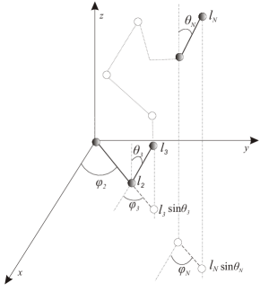
Figure 1: Three-dimensional conformation of a chain made of links and beads.

The calculation of the kinetic energy of the system $K_{disc}(t)$ in spherical coordinates is long but straightforward and gives as an upshot:

$$K_{disc} = \sum_{n=1}^{N}\sum_{k=1}^{n-1}\frac{m_{n}}{2}l^{2}_{n-k+1}\dot{\varphi}_{n-k+1}^{2}\sin^{2}\theta_{n-k+1}+\sum_{n=1}^{N}\sum_{k=1}^{n-1}\frac{m_{n}}{2}l^{2}_{n-k+1}\dot{\theta}^{2}_{n-k+1}$$ (2)

$$+ \sum_{n=1}^{N}\sum_{k=1}^{n-1}\sum_{i=2}^{n-k}m_{n}l_{i}l_{n-k+1}\left[\dot{\varphi}_{i}\dot{\varphi}_{n-k+1}\sin\theta_{i}\sin\theta_{n-k+1}\cos\left(\varphi_{n-k+1}-\varphi_{i}\right)\right.$$

$$+ \dot{\theta}_{i}\dot{\varphi}_{n-k+1}\cos\theta_{i}\sin\theta_{n-k+1}\sin\left(\varphi_{i}-\varphi_{n-k+1}\right)$$

$$+ \dot{\varphi}_{i}\dot{\theta}_{n-k+1}\sin\theta_{i}\cos\theta_{n-k+1}\sin\left(\varphi_{n-k+1}-\varphi_{i}\right)$$

$$+ \left.\dot{\theta}_{i}\dot{\theta}_{n-k+1}\left(\cos\theta_{i}\cos\theta_{n-k+1}\cos\left(\varphi_{n-k+1}-\varphi_{i}\right)+\sin\theta_{i}\sin\theta_{n-k+1}\right)\right]$$

To pass to the limit of a continuous chain we will use the rigorous procedure described in [7], where the two-dimensional case was analyzed. In order to do that, we assume that all segments have the same length and all beads have the same masses:

$$l_{i}=a\qquad(i=2,\ldots,N)\qquad\qquad m_{i}=\frac{M}{L}a\qquad(i=1,\ldots,N)$$ (3)

where $M=\sum\limits_{i=1}^{N}m_{i}$ and $L$ are the total mass and the total length of the chain respectively. The next step consists in performing the limit in which the continuous system is recovered:

$$a\longrightarrow 0\qquad N\longrightarrow+\infty\qquad Na=L$$ (4)

One can see from (4) that the product $Na$ is fixed and gives the total length of the chain. Exploiting Eqs. (2–4) it is possible to get the kinetic energy of the continuous chain. Let’s see for example how the recipe for performing the continuous limit works in the case of the third term in (2):

$$\sum_{n=1}^{N}\sum_{k=1}^{n-1}\sum_{i=2}^{n-k}m_{n}l_{i}l_{n-k+1}\dot{\varphi}_{i}\dot{\varphi}_{n-k+1}\sin\theta_{i}\sin\theta_{n-k+1}\cos(\varphi_{n-k+1}-\varphi_{i})$$ (5)

$$\longrightarrow \frac{M}{L}\sum_{n=1}^{N}a\sum_{k=1}^{n-1}a\sum_{i=2}^{n-k}a\dot{\varphi}(t,s_{i})\dot{\varphi}(t,s_{n}-s_{k}+a)$$

$$\times \sin\theta(t,s_{i})\sin\theta(t,s_{i}-s_{k}+a)\cos(\varphi(t,s_{i}-s_{k}+a)-\varphi(t,s_{i}))$$

$$\stackrel{{\scriptstyle a\rightarrow 0}}{{=}} \frac{M}{L}\int_{0}^{L}ds(L-s)\int_{0}^{s}dv\dot{\varphi}(t,v)\dot{\varphi}(t,s)\sin\theta(t,v)\sin\theta(t,s)$$

$$\times \cos(\varphi(t,s)-\varphi(t,v))$$

In obtaining the last part of the above equation we have exploited the formula

$$\int_{0}^{L}ds\int_{0}^{s}duf(u)=\int_{0}^{L}ds(L-s)f(s)$$ (6)

which is valid for any integrable function $f(s)$. Applying the prescription of Eq. (5) to the rest of the terms in Eq. (2), we get with the additional help of Eq. (6) the full expression of the kinetic energy of the continuos chain:

$$K(t) = \frac{M}{L}\int_{0}^{L}ds(L-s)\int_{0}^{s}dv\Big{[}\dot{\varphi}(t,v)\dot{\varphi}(t,s)\sin\theta(t,v)\sin\theta(t,s)$$ (7)

$$\times \cos\left(\varphi(t,s)-\varphi(t,v)\right)$$

$$+ \dot{\theta}(t,v)\dot{\varphi}(t,s)\cos\theta(t,v)\sin\theta(t,s)\sin\left(\varphi(t,v)-\varphi(t,s)\right)$$

$$+ \dot{\theta}(t,s)\dot{\varphi}(t,v)\sin\theta(t,v)\cos\theta(t,s)\sin\left(\varphi(t,s)-\varphi(t,v)\right)$$

$$+ \left.\dot{\theta}(t,v)\dot{\theta}(t,s)\Big{(}\cos\theta(t,v)\cos\theta(t,s)\cos\left(\varphi(t,s)-\varphi(t,v)\right)\right.$$

$$+ \sin\theta(t,v)\sin\theta(t,s)\Big{)}\Big{]}$$

We would like to stress that the right hand side of the derived equation contains five terms, while the initial discrete formula of the kinetic energy of Eq. (2) contained seven terms. This is due to the fact that the contributions from Eq. (2) in which $\dot{\varphi}^{2}_{n-k+1}$ and $\dot{\theta}^{2}_{n-k+1}$ are present disappear after taking the continuous limit because they are proportional to $a\longrightarrow 0$.

For future convenience, we give also the expression of the kinetic energy in cartesian coordinates:

$$K_{disc}=\sum_{i=2}^{N}\frac{m_{i}}{2}(\dot{x}_{i}^{2}+\dot{y}_{i}^{2}+\dot{z}_{i}^{2})$$ (8)

where $x_{i}$, $y_{i}$ and $z_{i}$ have been defined in Eq. (1). The sum over $i$ starts from $2$ because one end of the chain coincides with the origin of the axes, so that $l_{1}=0$. Of course, due to the condition that each segment has a fixed length $l_{i}$, Eq. (8) must be completed by the following constraints:

$$(x_{i}-x_{i-1})^{2}+(y_{i}-y_{i-1})^{2}+(z_{i}-z_{i-1})^{2}=l_{i}^{2}\qquad\qquad(i=2,\ldots,N)$$ (9)

At this point we have thus two choices. Either we keep the kinetic energy in the simple form of Eq. (8) at the price of having to deal with the constraints (9), or we solve those constraints using the spherical coordinates $l_{i},\theta_{i},\varphi_{i}$ of Eq. (1). In the latter case, the kinetic energy of Eq. (7) is both nonlocal and nonlinear and thus is difficult to be treated. In the continuous limit, the situation does not change substantially.

We end up this Section performing the continuous limit of the kinetic energy of Eq. (8) and of the constraints (9). Following the prescriptions given in Eqs. (3–4), we obtain:

$${\cal L}=\frac{M}{2L}\int_{0}^{L}ds\dot{\mathbf{R}}^{2}(t,s)$$ (10)

and

$$\mathbf{R}^{\prime 2}=1$$ (11)

where we have introduced the vector notation:

$$\mathbf{R}=[x(t,s),y(t,s),z(t,s)]$$ (12)

to describe the position on the chain. In polymer physics $\mathbf{R}$ is called the bond vector. In Eq. (10) and Eq. (11) we have put $\dot{\mathbf{R}}\equiv\frac{\partial\mathbf{R}}{\partial t}$ and $\mathbf{R}^{\prime}\equiv\frac{\partial\mathbf{R}}{\partial s}$.
The compatibility of the description in cartesian coordinates with that in spherical coordinates can be verified by introducing the fields $\theta(t,s),\varphi(t,s)$ connected with the cartesian fields $x(t,s),y(t,s),z(t,s)$ by the relations

$$x(t,s) = \int_{0}^{s}du\cos\varphi(t,u)\sin\theta(t,u)$$ (13)

$$y(t,s) = \int_{0}^{s}du\sin\varphi(t,u)\sin\theta(t,u)$$ (14)

$$z(t,s) = \int_{0}^{s}du\cos\theta(t,u)$$ (15)

If one performs the substitutions of Eqs. (13–15) in the kinetic energy (10) and makes use of the formula (6), one arrives exactly at the expression of the kinetic energy (7). Thus, Eq. (7) and Eq. (10) together with the constraint (11) are equivalent.

3 Dynamics of a chain immersed in a heat bath

In this Section the path integral formulation of an inextensible chain in the contact with a heat reservoir at temperature $T$ is provided. According to the construction presented in Sec. 2, the conformation of the chain is treated as the limit case of a system of $N$ beads connected by $N-1$ links of fixed length $a$. In the discrete case the positions of the beads are given by a set of three-dimensional cartesian vectors $\mathbf{R}_{n}(t)$, $(n=2,\ldots,N)$, while the conformation of the continuous chain at a given instant $t$ is described by the vector field $\mathbf{R}(t,s)$, $s$ being the arc–length. Furthermore, the chain is inextensible and thus has constant length $L=Na$.

In order to describe the thermodynamic fluctuations of the chain, we regard it as a system of $N$ Brownian particles of mass $m$ whose trajectories satisfy the constraints of Eq. (9). These constraints enforce the condition that the total length of the links connecting the beads should be equal to $a$. It is possible to rewrite Eq. (9) in the more compact form:

$$\frac{|\mathbf{R}_{n}(t)-\mathbf{R}_{n-1}(t)|^{2}}{a^{2}}=1\qquad\qquad(n=2,\ldots,N)$$ (16)

We also require that at the initial and final times $t=0$ and $t=t_{f}$ the position of $n$-th particle is respectively given by $\mathbf{R}_{n}(0)=\mathbf{R}_{0,n}$ and $\mathbf{R}_{n}(t_{f})=\mathbf{R}_{f,n}$ for $n=2,\ldots,N$.

In other words, the primary task of this Section is to analyze the dynamics of a system which consists in the constrained random walk of the beads composing the chain. The main difficulty in performing analytical calculations are obviously the constraints. Starting like in the Rouse model from an approach to the problem based on the Langevin equation to describe the motion of a polymer in a solution [11], the treatment of the constraints becomes awkward. For this reason we will use an interdisciplinary strategy, which combines the techniques of field theory with those used in the statistical mechanics of polymers with topological constraints. The starting point of the presented framework is to specify the probability distribution function $\Psi_{N}$ expressed in a path integral form. $\Psi_{N}$ contains the physical information about the system. To be more specific, it measures the probability that the chain after a given time $t_{f}$ passes from an initial configuration $\mathbf{R}_{0,n}$ to a final configuration $\mathbf{R}_{f,n}$.

Before we construct the probability function for the chain with rigid constraints, let’s see how the path integral of a single free Brownian particle looks like. In order to do this we assume that at the time $t=0$ the particle finds itself at the initial point $\mathbf{R}_{0}$ and starts to perform a random walk. As it is well known, the probability $\psi(t_{f};\mathbf{R}_{f},\mathbf{R}_{0})$ that, after the time $t_{f}$ the particle arrives at a given point $\mathbf{R}_{f}$, satisfies the diffusion equation

$$\frac{\partial\psi}{\partial t_{f}}=D\frac{\partial^{2}\psi}{\partial\mathbf{R}^{2}}$$ (17)

where $D$ is the diffusion constant. The boundary condition at $t_{f}=0$ is chosen in such a way that $\psi(0,\mathbf{R}_{f};\mathbf{R}_{0})=\delta(\mathbf{R}_{f}-\mathbf{R}_{0})$. The solution $\psi$ of (17) can be expressed in the form of a path integral

$$\psi(t_{f},\mathbf{R}_{f};\mathbf{R}_{0})=A\int_{\mathbf{R}(0)=\mathbf{R}_{0}}^{\mathbf{R}(t_{f})=\mathbf{R}_{f}}{\cal D}{\mathbf{R}}(t)\exp{\left[-\int_{0}^{t_{f}}\frac{\dot{\mathbf{R}}^{2}(t)}{4D}dt\right]}$$ (18)

where $A$ is a normalization factor. We note that the diffusion constant $D$ appearing in Eq. (18) satisfies the relation $D=\frac{kT\tau}{m}$, where $k$ is the Boltzmann constant, $T$ is the temperature of heat bath and $\tau$ is the relaxation time that characterizes the rate of decay of the drift velocity of the particle.

The above prescription can easily be generalized to a system of $N$ noninteracting Brownian particles. It this case the probability that the $n-$th particle starting from the point $\mathbf{R}_{0,n}$ arrives at the point $\mathbf{R}_{f,n}$ is given by

$$\psi_{N}=\prod_{n=1}^{N}\left[A\int_{\mathbf{R}_{n}(0)=\mathbf{R}_{0,n}}^{\mathbf{R}_{n}(t_{f})=\mathbf{R}_{f,n}}{\cal D}\mathbf{R}_{n}(t)\right]\exp{\left[-\frac{1}{2kT\tau}\sum_{n=1}^{N}\int_{0}^{t_{f}}\frac{m}{2}\dot{\mathbf{R}}_{n}^{2}(t)dt\right]}$$ (19)

In addition, the form of the path integral on the right hand side of Eq. (19) displays the connection with the partition function of a set of $N$ free particles in quantum mechanics where the functional ${\cal A}_{N}=\sum\limits_{n=1}^{N}\int_{0}^{t_{f}}\frac{m}{2}\dot{\mathbf{R}}_{n}(t)dt$ represents the action of the system. The well known duality between quantum mechanics and Brownian motions allows to treat the factor

$$\kappa=2kT\tau$$ (20)

as the quantity which plays the role of the Planck’s constant. Indeed, one may show that the uncertainties in the position and momentum of a Brownian particle due to the frequent collisions with the molecules in the solutions satisfy an analog of the Heisenberg uncertainty relations: $\Delta p\Delta r\sim\kappa$ [12].

Going back to the dynamics of an inextensible chain, the only difference with respect to a system of free particles is that the bond vector $\mathbf{R}_{n}(t)$ satisfies the additional constraints (16) restricting the trajectories of motion. To implement them in the dynamics of noninteracting Brownian particles we add a product of functional delta functions in the path integral (19) which imposes the desired conditions (16):

$$\Psi_{N} = C\left[\prod_{n=1}^{N}\int_{\mathbf{R}_{n}(0)=\mathbf{R}_{0,n}}^{\mathbf{R}_{n}(t_{f})=\mathbf{R}_{f,n}}{\cal D}\mathbf{R}_{n}(t)\right]e^{-\frac{M}{4k_{B}T\tau L}\sum_{n=1}^{N}a\int_{0}^{t_{f}}dt\dot{\mathbf{R}}_{n}^{2}(t)}$$ (21)

$$\times \prod_{n=2}^{N}\delta\left(\frac{\left|\mathbf{R}_{n}(t)-\mathbf{R}_{n-1}(t)\right|^{2}}{a^{2}}-1\right)$$

where $C$ is an irrelevant factor and the mass of a single particle present in Eq. (19) has been replaced according to the equation $m=\frac{M}{L}a$. The above procedure to fix the constraints in a path integral has been applied in the statistical mechanics of entangled polymers [13, 14, 15].
The next step consists in performing the continuous limit (4) in (21) [16]:

$$\Psi=\int_{\mathbf{R}(0,s)=\mathbf{R}_{0}(s)}^{\mathbf{R}(t_{f},s)=\mathbf{R}_{f}(s)}{\cal D}\mathbf{R}(t,s)e^{-\frac{1}{2kT\tau}\int_{0}^{t_{f}}dt\frac{M}{2L}\int_{0}^{L}ds\dot{\mathbf{R}}^{2}(t,s)}\delta(\mathbf{R}^{\prime 2}(t,s)-1)$$ (22)

The result of Eq. (22) defines a model which is closely related to the nonlinear sigma model (NL$\sigma$M) used in high energy physics [17], solid state physics [18] and disordered systems [19]. For this reason it has been called generalized nonlinear sigma model (GNL$\sigma$M). The most striking difference between these two models lays in the constraints, which in the case of the NL$\sigma$M are of the form $\mathbf{R}^{2}=1$, while in the GNL$\sigma$M they have been replaced by the nonholonomic condition (11).

To conclude this section let us note that it is possible to show that the generating functional of the correlation functions of the GNL$\sigma$M coincides with the generating functional of the correlation functions of the solutions of a constrained Langevin equation [8].

4 Dynamics of an inextensible chain with constant bending angle

The approach presented in Sec. 2 in order to treat the dynamics of random chains has some interesting variants which we would like to discuss in this Section. To this purpose, we choose the formulation in which the positions of the ends of the segments composing the chain are given in cartesian coordinates. As we have already seen, in this way the expression of the kinetic energy $K_{disc}$ is given by (8) and must be completed by the constraints (9). From now on we assume as before that all segments have the same fixed length $l_{n}=a$, but we require additionally that:

$$(z_{n}-z_{n-1})^{2}=b^{2}\leq a^{2}$$ (23)

This implies that the projection of each segment onto the $z-$axis has length $\pm b$, so that the segments are bound to form with the $z-$axis the fixed angles $\alpha_{1}=\alpha$ or $\alpha_{2}=(\pi-\alpha)$ defined by the relations:

$$\cos\alpha_{1}=+\frac{b}{a}\qquad\qquad\cos\alpha_{2}=-\frac{b}{a}$$ (24)

Clearly, in both cases the constraints (9) and (23) may be rewritten as follows:

$$\frac{(x_{n}-x_{n-1})^{2}}{b^{2}}+\frac{(y_{n}-y_{n-1})^{2}}{b^{2}}=\frac{1}{\cos^{2}\alpha}-1\qquad\qquad(n=2,\ldots,N)$$ (25)

where $\alpha$ may be either $\alpha_{1}$ or $\alpha_{2}$. In the following we will suppose that only the angle $\alpha=\alpha_{1}$ is allowed, so that the chain cannot make turns in the $z$ direction. An example of a conformation of a chain satisfying these assumptions is given in Fig. 2.

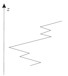
Figure 2: Example of motion of a chain whose segments are constrained to form a fixed angle $\alpha$ with the $z-$axis. In the figure $\alpha=30^{\circ}$.

The constraints (25) are eliminated using the spherical coordinates of Eq. (1) after setting the angles $\theta_{n}$ formed by the segments with the $z-$axis equal to $\alpha$:

$$x_{n}(t) = \sum_{i=1}^{n}l_{i}\cos\varphi_{i}(t)\sin\alpha$$ (26)

$$y_{n}(t) = \sum_{i=1}^{n}l_{i}\sin\varphi_{i}(t)\sin\alpha$$ (27)

$$z_{n}(t) = \sum_{i=1}^{n}l_{i}\cos\alpha=na\cos\alpha$$ (28)

As we see from the above equation, each segment is left only with the freedom of rotations around the $z-$direction, corresponding to the angles $\varphi_{i}(t)$. Moreover, the total length of the chain is always $L=Na$, but now also the total height $h$ of the trajectory along the $z-$axis is fixed:

$$h=Nb$$ (29)

At this point, we pass to the continuous limit, this time taking as parameter describing the trajectory of the chain the variable $z$ instead of the arc-length $s$. Due to the last of Eqs. (28), the $z-$components of the velocities are always zero:

$$\dot{z}_{n}(t)=0$$ (30)

As a consequence, we are left with something similar to a two-dimensional problem. The difference from a real two-dimensional problem, which could be obtained by putting $\theta_{j}=\pi/2$ ($j=1,\ldots,N$) in Eq. (1), is that the equations describing the position of a bead in two dimensions, namely $x_{i}(t)=\sum_{j=1}^{N}l_{j}\cos\varphi_{j}(t)$ and $y_{i}(t)=\sum_{j=1}^{N}l_{j}\sin\varphi_{j}(t)$, have been replaced by Eqs. (26) and (27). Moreover, the constraints have a slightly different form. Following the same procedure presented in Sec. 2, we find after a few calculations the expression of the kinetic energy in the continuous limit:

$$K_{\alpha} = \tan^{2}\alpha\frac{M}{2h}\int_{0}^{h}dz\int_{0}^{z}dz_{1}\int_{0}^{z_{1}}dz_{2}$$ (31)

$$\times \dot{\varphi}(t,z-z_{1})\dot{\varphi}(t,z_{2})\cos(\varphi(t,z-z_{1})-\varphi(t,z_{2}))$$

and of the constraint (25):

$$(\partial_{z}x)^{2}+(\partial_{z}y)^{2}=\tan^{2}\alpha$$ (32)

It is also not difficult to show that the probability distribution $\Psi_{\alpha}$ is given in cartesian coordinates by:

$$\Psi_{\alpha}=\int{\cal D}x(t,z){\cal D}y(t,z)\exp\left\{-\frac{{\cal A}_{\alpha}}{\kappa}\right\}\delta((\partial_{z}x)^{2}+(\partial_{z}y)^{2}-\tan^{2}\alpha)$$ (33)

where

$${\cal A}_{\alpha}=\frac{M}{2h}\int_{0}^{t_{f}}dt\int_{0}^{h}dz\left[\dot{x}^{2}(t,z)+\dot{y}^{2}(t,z)\right]$$ (34)

At this point we discuss briefly the case in which both angles $\pi-\alpha$ and $\alpha$ are allowed. In this situation, the trajectory of the chain may have turns. An example of motion of this kind is given in Fig. 3.

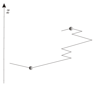
Figure 3: Example of motion of a chain whose segments are constrained to form fixed angles $\alpha$ or $\pi-\alpha$ with the $z-$axis. In the figure $\alpha=30^{\circ}$. Turning points are emphasized by means of shaded beads.

The constraints (9) and (23) remain unchanged, but the coordinate $z$ cannot be chosen as a valid parameter of the trajectory of the chain and one has to come back to the arc-length $s$. The most serious problem is the fact that the variables $z_{n}(t)$ are not continuous functions of the time, since the length $z_{n}(t)-z_{n-1}(t)$ is allowed to jump discretely between the two discrete values $+b$ and $-b$, corresponding to the angles $\alpha$ and $\pi-\alpha$ respectively. It is therefore difficult to define the components $\dot{z}_{n}$ of the velocities of the ends of the segments and thus their contribution to the kinetic energy. Let us note that this problem affects only the $z$ degrees of freedom. The degrees of freedom $x_{n}(t)$ and $y_{n}(t)$ of the chain remain continuous functions of $t$ despite the jumps of the $z_{n}$’s. This fact can be easily verified looking at the definition of $x_{n}(t)$ and $y_{n}(t)$ in Eqs. (26) and (27). Since $\sin(\pi-\alpha)=\sin\alpha$, both the $x_{n}(t)$’s and $y_{n}(t)$’s are not affected by the jumps of the angle $\alpha\longleftrightarrow\pi-\alpha$. As a consequence, the problems with the $z$ variable can easily be solved if the chain has no interactions in which the $z$ variable is involved. In this case, in fact, the degrees of freedom connected to the motion along the $z-$direction are decoupled from the other degrees of freedom and may be neglected.

As a consequence, we assume that the interactions are $z-$independent, so that the difficulties related to the motion along the $z-$direction disappear and once again the problem reduces to that that of a two-dimensional chain. Since the constraints are always those of Eqs. (9) and (23), one may proceed as in the case of fixed angle $\alpha$. As a result, one finds that the final probability distribution is of the form:

$$\Psi_{\alpha,\pi-\alpha} =$$ (35)

$$\!\!\!\!\!\!\!\!\!\!\!\!\!\!\!\!\!\!\!\!\!\!\!\!\!\!\!\!\!\!\!\!\!\!\!\!\!\!\!\!\!\!\!\!\!\!\!\!\!\!\!\!\!\!\!\!\!\!\!\!{\cal C}\int{\cal D}x(t,s){\cal D}y(t,s)\exp\left\{-\frac{{\cal A}_{\alpha,\pi-\alpha}}{\kappa}\right\}\delta((\partial_{s}x)^{2}+(\partial_{s}y)^{2}-\tan^{2}\alpha)$$

where

$${\cal A}_{\alpha,\pi-\alpha}=\frac{M}{2L}\int_{0}^{t_{f}}dt\int_{0}^{L}ds\left[\dot{x}^{2}(t,s)+\dot{y}^{2}(t,s)\right]$$ (36)

and ${\cal C}$ is a constant containing the result of the integration over the decoupled $z$ degrees of freedom. With respect to the previous case, let us note that in Eqs. (35) and (36) $z$ has been replaced by the arc-length $s$ as the parameter of the trajectory of the chain. Correspondingly, the total chain length $L$ appears in the action instead of the height $h$.

5 Conclusions

In this work the dynamics of an inextensible freely jointed chain consisting of links and beads in three dimensions has been discussed both from the classical and statistical point of view. In Sec. 2 we have mainly concentrated ourselves on the computation of the kinetic energy in cartesian and spherical coordinates for the discrete and continuous chain. In Sec. 3 we have derived the probability function of the chain $\Psi$ using a path integral framework and the fact that the fluctuations of the chain can be regarded as those of a system of Brownian particles with an additional constraint condition imposed on their trajectories. The probability function $\Psi$ of this system is equivalent to the partition function of a generalized nonlinear $\sigma$ model. The analogy of the GNL$\sigma$M with the NL$\sigma$M suggests the possibility of applying techniques and results coming from the NL$\sigma$M to the GNL$\sigma$M. For example, it is known that the NL$\sigma$M is renormalizable in two dimensions and also that it has interesting features because it is analytically free and has a dynamically generated mass gap [20]. The similarity with NL$\sigma$M seems also to suggest that there is no symmetry breaking in the underlying $O(d)$ symmetry of the GNL$\sigma$M, where $d$ denotes the dimension of the vector field $\mathbf{R}(t,s)$. One should however be careful when extending the results of the NL$\sigma$M to the GNL$\sigma$M. For example if $d=2$, one may use polar field coordinates to express the vector field $\mathbf{R}(t,s)$. If one does that the NL$\sigma$M becomes a free field theory in the angle variable [21]. This is not true in the case of the GNL$\sigma$M which in polar coordinates exhibits a nonlinear and complicated dependence on the angle degree of freedom. Moreover, it is not straightforward to apply techniques like the effective potential method which is useful to investigate possible phase transitions in the NL$\sigma$M. The reason is that in this method it is performed an expansion around field configurations minimalizing the action which are constant. Configurations of this kind correspond in the GNL$\sigma$M to the situation in which the chain has collapsed to a point and thus are nonphysical. Finally in Sec. 4 a three-dimensional chain admitting only fixed angles with respect to the $z-$axis has been discussed. It has been shown that it is possible to reduce the problem to two dimensions, in a way which is similar to the reduction of the statistical mechanics of a directed polymer to the random walk of a two-dimensional particle [22]. Our approach is valid only if the chain has no turning points. If there are turning points the kinetic energy is not well defined, because the variable $z(t,s)$ is no longer a continuous function and thus its time derivative becomes a distribution. One way for adding to our treatment turning points as those of Fig. 3 is to replace the variable $z$ with a stochastic variable which is allowed to take only discrete values. Another way is to look at turning points as points in which the chain bounces against an invisible obstacle. A field theory describing a one-dimensional chain with such kind of constraints has been already derived in Refs. [23].

6 Acknowledgements

This work has been financed by the Polish Ministry of Science and Higher Education, scientific project N202 156 31/2933. The authors wish to thank the anonymous referee for useful comments.

References

- [1] S. F. Edwards and A. G. Goodyear, J. Phys. A: Gen. Phys. 5 (1972), 965.
- [2] S. F. Edwards and A. G. Goodyear, J. Phys. A: Gen. Phys. 5 (1972), 1188.
- [3] S. F. Edwards and A. G. Goodyear, J. Phys. A: Gen. Phys. 6 (1973), L31.
- [4] H. C. Öttinger, Phys. Rev. E 50 (1994), 2696.
- [5] D. Petera and M. Muthukumar, J. Chem. Phys. 111 (1999), 7614.
- [6] H. M. Ådland and A. Mikkelsen, J. Chem. Phys. 120 (2004), 9848.
- [7] F. Ferrari, J. Paturej and T. A. Vilgis, Phys. Rev. E 77 (2008), 021802.
- [8] F. Ferrari and J. Paturej, J. Phys. A 42, 145002.
- [9] F. Ferrari, J. Paturej and T. A. Vilgis, Applications of a generalization of the nonlinear sigma model with group of symmetry to the dynamics of a constrained chain, arXiv:0807.4045 (submitted to Nucl. Phys. B)
- [10] F. Ferrari, J. Paturej, T. A. Vilgis and T. Wydro, The probability distribution of the average relative distance between two points in a dynamical chain, arXiv:0809.2261 (submitted to J. Chem. Phys.)
- [11] M. Doi and S.F. Edwards, The Theory of Polymer Dynamics (Clarendon Press, Oxford, 1986).
- [12] S. A. Rice and H. L. Frisch, Ann. Rev. Phys. Chem. 11 (1960), 187.
- [13] F. Ferrari, H. Kleinert and I. Lazzizzera, Int. Jour. Mod. Phys. B 14 (1998), 3881.
- [14] A. L. Kholodenko and T. A. Vilgis, Phys. Rep. 298 (1998), 251.
- [15] M. G. Brereton and T. A. Vilgis, J. Phys. A: Math. Gen. 28 (1995), 1149.
- [16] H. Kleinert, Gauge Fields in Condensed Matter (World Scientific, Singapore, 1990), Vol. 1.
- [17] S. Weinberg, Phys. Rev. Lett. 18 (1967), 188; Phys. Rev. 166 (1968), 1568.
- [18] P. B. Wiegmann, J. Phys. C: Solid State Phys. 11 (1978), 1583; F. D. Haldane, Phys. Rev. Lett. 61 (1988), 1029.
- [19] V. R. Kogan, K. B. Efetov, Phys. Rev. B 67 (2003), 245312; K. Takahashi, Phys. Rev. E 70 (2004), 066147.
- [20] J. O. Andersen, D. Boer and H. J. Warringa, Phys. Rev. D 69 (2004), 076006.
- [21] J. Zinn-Justin, Quantum Field Theory and Critical Phenomena, (Clarendon Press, Oxford, 2002).
- [22] R. D. Kamien, P. Le Doussal and D. R. Nelson, Phys. Rev. A 45 (1992), 8727.
- [23] H. Arodź, P. Klimas and T. Tyranowski, Phys. Rev. E 73 (2006); Acta Phys. Pol. B 38 (2007), 2537; Acta Phys. Pol. B 36 (2005), 3861; H. Arodź, Acta Phys. Pol. B 33 (2002), 1241; H. Arodź, Acta Phys. Pol. B 35 (2004), 625.