Beauty and charm results from $B$-factories

Abstract

We present the proceedings of the lectures given at the 2008 Helmholtz International Summer School Heavy Quark Physics at the Bogoliubov Laboratory of Theoretical Physics in Dubna. In two lectures we present recent results from the existing $B$-factories experiments, Belle and BaBar. The discussed topics include short phenomenological motivation, experimental methods and results on $B$ meson oscillations, selected rare $B$ meson decays (leptonic, $b\to s\gamma$ and $b\to s\ell^{+}\ell^{-}$), mixing and $CP$ violation in the system of $D^{0}$ mesons, and leptonic decays of $D_{s}$ mesons.

1 Introduction

The lectures presented in this paper are a part of the $B$-factories lectures prepared in collaboration with A.J. Bevan (also given in the proceedings of the school, [1]). To obtain an approximate overview of recent results on flavour physics arising from Belle and BaBar both sets of presentations (each composed of two one-hour lectures) should be consulted.

The lectures presented here include - beside the experimental methods and results - some short phenomenological sketches of motivation and/or interpretation of individual measurements. The author, being an experimentalist, should warn the reader that some examples of phenomenological interpretation are simplified and that serious theoretical treatment requires consultation of references given in the text. Examples are thus to be treated with a grain of salt; to quote the famous poet: ”It is a curious fact that people are never so trivial as when they take themselves seriously.” (O. Wilde, 1854 - 1900).

A large majority of results presented in the lectures arise from the measurements performed with the two experiments taking data at the $B$-factories, $e^{+}e^{-}$ asymmetric colliders running at the center-of-mass (CM) energy $\sqrt{s}=m_{\Upsilon(4S)}c^{2}$ . $\Upsilon(4S)$, a $b\bar{b}$ bound state with a mass just above the threshold for $\Upsilon(4S)\to B\bar{B}$ decay, is a copious source of $B$ meson pairs. Mesons are produced almost at rest in the CM system, but since the electron beam has an energy higher than the positron one, they are boosted and decay time dependent measurements of meson decays are thus possible. The Belle detector [2], operating at the KEKB collider [3] in Tsukuba, Japan, has so far recorded an integrated luminosity of around 860 fb^-1, roughly corresponding to $950\times 10^{6}$ pairs of $B$ mesons . The BaBar detector [4] at the PEP-II collider in Stanford, USA, has recorded around 550 fb^-1 of data.

Beside the production of $B$ meson pairs from the $\Upsilon(4S)$ other processes take place in $e^{+}e^{-}$ collisions at the given CM energy. For the subject of the lectures the most important is the continuum production of $c\bar{c}$ quark pairs, arising in $e^{+}e^{-}\to\gamma^{\ast}\to c\bar{c}$. This is sketched in Fig. 1, where the cross-section for hadron production in electron-positron collisions is plotted as a function of the CM collision energy.

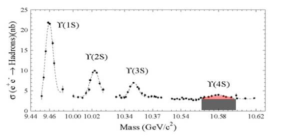
Figure 1: Cross-section for production of hadrons in $e^{+}e^{-}$ collisions as a function of $\sqrt{s}$. The resonant production of $\Upsilon(4S)\to B\bar{B}$ is represented as the light shaded area, and the continuum $e^{+}e^{-}\to\gamma^{\ast}\to q\bar{q}$ as the dark shaded area.

The cross-section for the production of $c\bar{c}$ pairs is larger than the one for the $B$ meson production, at the integrated luminosity of KEKB it corresponds to around $1.1\times 10^{9}$ produced pairs of charmed hadrons.

In the course of the lectures we will mention also some related results from experiments other than $B$-factories, specifically the ones from the CDF-II experiment at Tevatron [5], recording data in $p\bar{p}$ collisions, and Cleo-c experiment [6] at the $e^{+}e^{-}$ collider CESR, running at the $D\bar{D}$ meson pair production threshold. All these experiments provide for a truly diverse experimental environment to study various aspects of heavy flavour physics. ”We all live with the objective of being happy; our lives are all different and yet the same.” (A. Frank, 1929 - 1945).

2 Lecture I

”Never loose an opportunity of seeing anything beautiful, for beauty is God’s handwriting.” (R.W. Emerson, 1803-1882)

2.1 $B$ meson oscillations

The mixing of neutral mesons, that is the transition of a neutral meson $P^{0}$ into its antiparticle and vice-versa, appears as a consequence of states of definite flavour ($P^{0}$, $\bar{P}^{0}$) being a linear superposition of the eigenstates of an effective Hamiltonian (states of a simple exponential time evolution) $P_{1,2}$:

$$|P_{1,2}\rangle=p|P^{0}\rangle\pm q|\bar{P}^{0}\rangle~{}~{}.$$ (1)

For a thorough derivation of the equations describing the oscillations of mesons the reader is advised to follow [7].

While the mass eigenstates have a simple time evolution, the time dependent decay rate of flavour eigenstates depends on the mixing parameters $x$ and $y$, expressed in terms of the mass and width difference of $P_{1,2}$ as $x=(m_{1}-m_{2})/\bar{\Gamma}$ and $y=(\Gamma_{1}-\Gamma_{2})/2\bar{\Gamma}$. $\bar{\Gamma}$ is the average decay width of the two mass eigenstates. The decay rate of a state initially produced as a $P^{0}$ is

$$\frac{d\Gamma(P^{0}\to f)}{dt}=e^{-t}\bigl{[}\bigl{(}|A_{f}|^{2}+|\frac{q}{p}\bar{A}_{f}|^{2}\bigr{)}\cosh{yt}+\bigl{(}|A_{f}|^{2}-|\frac{q}{p}\bar{A}_{f}|^{2}\bigr{)}\cos{xt}$$

$$+2\Re{\bigl{(}\frac{q}{p}A_{f}^{\ast}\bar{A}_{f}\bigr{)}}\sinh{yt}-2\Im{\bigl{(}\frac{q}{p}A_{f}^{\ast}\bar{A}_{f}\bigr{)}}\sin{xt}\bigr{]}~{}.$$ (2)

In the above equation $t$ is a dimensionless decay time, defined in terms of a proper decay time $t^{\prime}$ as $t=t^{\prime}\bar{\Gamma}$. The notation $A_{f},~{}\bar{A}_{f}$ is used to represent instantaneous amplitudes for $P^{0}\to f$ and $\bar{P}^{0}\to f$ decays. It is obvious from Eq. (2) that using the decay time distribution of experimentally accessible flavour eigenstates one can determine the mixing parameters $x$ and $y$. Moreover, the effect of the mixing parameters on $d\Gamma/dt$ depends on the chosen decay channel ($A_{f},~{}\bar{A}_{f}$). The decay time distribution of an initially produced $\bar{P}^{0}$ is obtained from Eq. (2) by replacing $A_{f}\leftrightarrow\bar{A}_{f}$ and $q/p\to p/q$. The decay time distributions for decays to conjugated final state $\bar{f}$ are obtained by a simple $f\to\bar{f}$ transformation. The above decay rates are illustrated in Fig. 2 for several values of $x$ and $y$.

Figure 2: Probability for an initially produced meson $P^{0}$ to decay at time $t$ as $P^{0}$ (full curve) or $\bar{P}^{0}$ (dashed curve). Qualitatively the left example roughly corresponds to the case of $B_{s}^{0}$ mesons, the middle one to the case of $B^{0}$ mesons and the right one to the case of $D^{0}$ mesons. Note the logarithmic scale on the right plot.

The neutral $B$ meson pairs from $\Upsilon(4S)$ decays are produced in a quantum coherent state with the quantum numbers corresponding to that of the $\Upsilon(4S)$. Before the coherence is disturbed by a decay of one of the mesons, the pair is always in a $B^{0}-\bar{B}^{0}$ state. The decay rates given above are valid only after the first of the two mesons decays. To be used in measurements of $B^{0}$ mesons produced from $\Upsilon(4S)$, the decay time $t$ in Eq. (2) should thus be changed to $\Delta t$, the difference between the decay times of the first and the second neutral $B$ meson (and the exponential factor should include $|\Delta t|$ instead of $t$).

The experimental method of measuring $B^{0}$ meson oscillation frequency $x$ relies on a similar method as the one used for measuring the $CP$ violation [1]. However, instead of $CP$ specific final states, flavour specific final states of $B$ meson decays are used (like $B^{0}\to J/\psi K^{\ast 0},~{}K^{\ast 0}\to K^{+}\pi^{-}$), which allow to determine the flavour of the decaying $B$ meson. The method is sketched in Fig. 3. The measured $\Delta t$ distribution deviates from Eq. (2) due to several reasons: usage of flavour specific final state ($\bar{A}_{f}=A_{\bar{f}}=0$), negligible decay width difference ($y\ll 1$), probability of wrong flavour tagging ($w$) and finite accuracy in determination of $\Delta t$ (resolution function $R_{\rm sig}(\Delta t)$). Taking into account these corrections, the final expected decay time distributions are

$$\frac{d\Gamma(B^{0}\to f)}{d\Delta t}=e^{-|\Delta t|}|A_{f}|^{2}\bigl{[}1+(1-2w)\cos(x\Delta t)\bigr{]}\otimes R_{\rm sig}(\Delta t)$$

$$\frac{d\Gamma(\bar{B}^{0}\to f)}{d\Delta t}=e^{-|\Delta t|}|A_{f}|^{2}\bigl{[}1-(1-2w)\cos(x\Delta t)\bigr{]}\otimes R_{\rm sig}(\Delta t)~{}~{},$$ (3)

where the $\otimes$ sign denotes a convolution. The resolution function is composed as a convolution of several Gaussian functions [8]. The average accuracy of $\Delta t$ determination is around 1.4 ps (the lifetime of $B^{0}$ mesons is 1.53 ps [9]).

Figure 3: Illustration of the method used to measure the $B^{0}$ oscillation frequency $x$.

The most precise single measurement of $x$ [10] uses several flavour specific final states to reconstruct the signal $B^{0}$ meson decays. Results are presented in Fig. 4 (left) in form of the asymmetry

$$\frac{d\Gamma(B^{0}\to f)/d\Delta t-d\Gamma(\bar{B}^{0}\to f)/d\Delta t}{d\Gamma(B^{0}\to f)/d\Delta t+d\Gamma(\bar{B}^{0}\to f)/d\Delta t}=(1-2w)\cos{x\Delta t}\otimes R_{\rm sig}(\Delta t)~{}~{}.$$ (4)

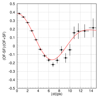
Figure 4: Left: Result of $B^{0}$ oscillation frequency measurement [10] shown in the form of the asymmetry (4). Right: Loop diagram describing the $B^{0}\to\bar{B}^{0}$ transition (top) and the short distance contribution to $D^{0}\to\bar{D}^{0}$ (bottom) transition.

The average value of existing $\Delta m$ measurements [11], expressed in terms of $x=\Delta m/\bar{\Gamma}$, is $x=0.776\pm 0.008$.

Calculation of $\langle\bar{B}^{0}|H_{eff}|B^{0}\rangle$ matrix element, visualized by the loop diagram of Fig. 4 (right), results in [12]

$$\Delta m_{q}=2\frac{G_{F}^{2}m_{W}^{2}\eta_{B}m_{B_{q}}B_{B_{q}}f_{B_{q}}^{2}}{12\pi^{2}}S_{0}(m_{t}^{2}/m_{W}^{2})|V_{tq}^{\ast}V_{tb}|^{2}\bigl{(}1+{\cal{O}}(\frac{m_{b}^{2}}{m_{t}^{2}})\bigr{)}~{}.$$ (5)

The equation is written using a subscript $q$ to emphasize that the same relation is also appropriate for the system of $B_{s}^{0}$ mesons. Using the measured value of the oscillation frequency for $B^{0}$ mesons one can determine elements of the Cabibbo-Kobayashi-Maskawa (CKM) matrix, if the QCD parameters $\eta_{B},~{}B_{B_{q}},~{}f_{B_{q}}$ are known. Due to their non-perturbative nature these quantities are difficult to estimate (usualy the lattice QCD calculations, LQCD, are exploited) and result in a large uncertianty of CKM elements determination. The constraints from the measured value of $\Delta m$ on parameters $(\bar{\rho},\bar{\eta})$ used to parametrize the CKM matrix [13] are shown in Fig. 5 (left) [14]. Since 2006 the oscillation frequency is measured also in the system of $B_{s}^{0}$ mesons, $x_{s}=25.5\pm 0.6$ [15]. In the ratio of $\Delta m_{s}/\Delta m$ the QCD uncertainties cancel to a large extent. The measured ratio $\Delta m_{s}/\Delta m$ is thus much more constraining than $\Delta m$ constraint alone (Fig. 5 (left)), and actually at the moment represents the most constraining measurement for the $\bar{\rho}$ among various flavour physics studies.

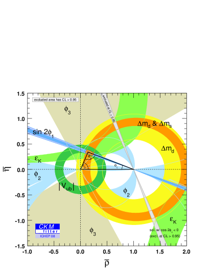
Figure 5: Left: Constraints in the $(\bar{\rho},\bar{\eta})$ plane arising from various measurement [14]. The light shaded region denoted by $\Delta m_{d}$ represents the constraint from the $B^{0}$ oscillation frequency, and the dark shaded region denoted by $\Delta m_{d}\&\Delta m_{s}$ the constraint from the ratio of $B^{0}$ and $B_{s}^{0}$ oscillation frequencies. Right: Feynman diagram of a pseudoscalar meson leptonic decay. The QCD effects are described by the decay constant $f_{P}$. Beside the SM $W^{+}$ contribution also particles not included in the SM (like the charged Higgs boson) may contribute.

2.2 Leptonic $B$ meson decays

Measurements of charged $B$ meson leptonic decays are interesting for several reasons: theoretically they are easier to interpret compared to semileptonic and hadronic decays, within the SM the measured rates can potentially yield the value of the least known CKM element $V_{ub}$, and they are sensitive to possible contributions of processes beyond the SM. A Feynman diagram of an arbitrary pseudoscalar meson leptonic decay is shown in Fig. 5 (right). The QCD effects are described by a single parameter $f_{P}$, the meson decay constant describing the overlap of the two quarks wave function.

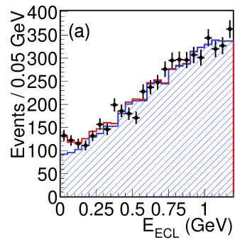
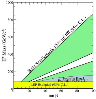
Figure 6: Left: Distribution of the energy in the electromagnetic calorimeter for selected $B^{+}\to\tau^{+}\nu_{\tau}$ candidate events. The excess of data (points with error bars) above the expectation from simulation (histogram) is the signal. Right: Excluded region (shaded) in the $(m_{H},\tan\beta)$ plane arising from the measurement of $Br(B^{+}\to\tau^{+}\nu_{\tau})$ [16].

The leptonic decays of a pseudoscalar mesons are helicity suppressed, the expected ratios of decay widths are $1:4\times 10^{-3}:10^{-7}$ for the $\tau,\mu$ and $e$ decays, respectively. Despite the problems due to at least two undetected neutrinos in the final state the decays to $\tau$ leptons are the only decays observed so far.

The method of measurement consist of fully (partially) reconstructing the accompanying $B$ meson using a large number of hadronic (semileptonic) decay modes. After the particles assigned to the tagging meson are successfully identified one searches for one or three charged tracks originating from the $\tau$ decay. Finally the energy in the electromagnetic calorimeter ($E_{\rm ECL}$) not assigned to the particles used in the previous reconstruction is examined. Signal decays with only neutrinos left in the final state are expected to peak at $E_{ECL}\sim 0$. The $E_{\rm ECL}$ distribution of selected events in the measurement by Belle [16] is shown in Fig. 6 (left). The excess of events above the expectation from MC simulation at low values of $E_{\rm ECL}$ is the signal for the $B^{+}\to\tau^{+}\nu_{\tau}$ decays. From the fit to the distribution the branching fraction $Br(B^{+}\to\tau^{+}\nu_{\tau})=(1.65\pm^{0.38}_{0.37}\pm^{0.35}_{0.37})\times 10^{-4}$ is obtained, where the main contribution to the systematic error arises from the uncertainties in the shape of the $E_{\rm ECL}$ signal and background distributions. A similar measurement performed by BaBar [17] yields $Br(B^{+}\to\tau^{+}\nu_{\tau})=(1.2\pm 0.4\pm 0.4)\times 10^{-4}$, and iclusion of the Belle measurement using the hadronic tagging [18] results in the average of all measurements provided by Heavy Flavour Averaging Group, $Br(B^{+}\to\tau^{+}\nu_{\tau})=(1.51\pm 0.33)\times 10^{-4}$ [11] .

Calculation of $\Gamma(B^{+}\to\tau^{+}\nu_{\tau})$ yields [20]

$$\Gamma(B^{+}\to\tau^{+}\nu_{\tau})=\frac{G_{F}^{2}}{8\pi}|V_{ub}|^{2}f_{B}^{2}m_{B}m_{\tau}^{2}(1-\frac{m_{\tau}^{2}}{m_{B}^{2}})^{2}\bigl{[}1-\frac{m_{B}^{2}}{m_{H}^{2}}\tan^{2}\beta\bigr{]}^{2}~{}~{},$$ (6)

where the last factor in brackets is a correction due to a possible contribution of the charged Higgs boson. The measured value is in agreement with the SM expectation (using LQCD prediction $f_{B}=(216\pm 22)$ MeV [21], and $|V_{ub}|=(3.9\pm 0.5)\times 10^{-}3$ [20]) and allows to put constraints on the parameters $(m_{H},\tan\beta)$ in the two Higgs doublet models ($m_{H}$ is the charged Higgs boson mass and $\tan\beta$ is the ratio of the vacuum expectation values). The constraints arising from the Belle measurement are shown in Fig. 6 (right).

2.3 $b\to s\gamma$ decays

Decays involving the $b\to s\gamma$ transition cannot occur at the tree level in SM. Such a flavor changing neutral current (FCNC) is only possible as a higher order process and is thus sensitive to possible contributions of New Physics (NP). Some possible diagrams, within and beyond the SM, are shown in Fig. 7 (left). At the parton level the photon energy in the CM frame is approximately half of the $b$ quark mass. Also at the hadron level $E_{\gamma}$ is sensitive to $m_{b}$, which is important for determination of $|V_{ub}|$ and $|V_{cb}|$ from semileptonic $B$ decays.

There are both, theoretical and experimental difficulties in the measurements. The former arise since in all experimental methods there is a lower cut-off applied to $E_{\gamma}$. To determine the branching fraction, for example, one has to extrapolate the partial rate for $E_{\gamma}>E_{\rm cut}$ to the full energy region using models, which introduces theoretical uncertainties. On the experimental side the efforts are being made to lower the cut-off, but this makes problems due to the huge backgrounds even more severe (see Fig. 7 (right)). The name of the game is thus to suppress the backgrounds to an acceptable level; ”Your background and environment is with you for life. No question about that.” (S. Connery, 1930).

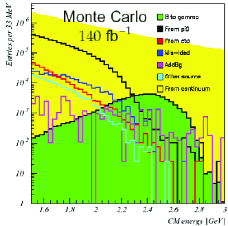
Figure 7: Left: SM (top) and some NP (middle and bottom) contributions to the $b\to s\gamma$ process. Right: Simulated photon energy distributions from various processes. The smallest shaded region is the contribution of $b\to s\gamma$ (note the logarithmic scale).

Methods of reconstruction may be divided into inclusive, semi-inclusive and exclusive ones. In an inclusive measurement only the photon is reconstructed. From the total $E_{\gamma}$ distribution of events recorded at the $\Upsilon(4S)$ peak an analogous distribution of events, recorded 60 MeV below the peak is subtracted. The latter represents only the photons arising from $e^{+}e^{-}\to q\bar{q}$ (continuum) events, and if the distribution is scaled according to the integrated luminosity of both samples, the remainder after the subtraction represents the energy distribution of photons from $B$ meson decays. A search is made for photon pairs consistent with $\pi^{0}$ or $\eta$ decays and such $\gamma$’s are removed from the selected sample. The remaining background is estimated using simulated samples but normalized using data control samples.

Result of such an inclusive method is shown in Fig. 8 (left) [22].

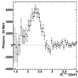
Figure 8: Left: Raw CM system photon energy distribution for inclusively reconstructed $b\to s\gamma$ decays [22]. Right: Differential branching fraction of $B\to X_{s}\gamma$ as a function of $E_{\gamma}$ obtained in semi-inclusive measurement [23].

$E_{\gamma}$ distribution peaks at around half of the $b$ quark mass and is consistent with zero above the kinematic limit for $B\to K\gamma$ decays, confirming the correctness of the subtraction procedure. To determine the branching fraction and the correct shape of the energy distribution one has to apply a deconvolution method to the raw spectrum, correct it for the efficiency of reconstruction, subtract a simulated contribution of $b\to d\gamma$ decays ($\sim$4%) and make the transformation to the $B$ meson rest frame. The partial branching fraction in the interval $E_{\gamma}>1.7$ GeV is found to be $Br(b\to s\gamma)=(3.31\pm 0.19\pm 0.37\pm 0.01)\times 10^{-4}$. The last uncertainty is due to the boost from the CM to the $B$ meson frame, and the largest systematic uncertainty arises from the normalization of backgrounds other than $\pi^{0}$ and $\eta$.

As an example of a semi-inclusive measurement we present the analysis of $B\to X_{s}\gamma$ by BaBar collaboration [23], where $X_{s}$ represent a sum of various decay modes with $K^{\pm},~{}K_{S},~{}\pi^{\pm}$ and $\eta$ mesons in the final state. The photon energy is in this method calculated from the invariant mass of the hadronic system $m(X_{s})$ which results in a better resolution compared to the measured photon energy in the electromagnetic calorimeter. The background is suppressed using neural network for the rejection of continuum events and vetoes for $\gamma$’s from $\pi^{0}$ and $\eta$ mesons. To calculate the branching fraction for $B\to X_{s}\gamma$ the number of observed events must be corrected for the fraction of decays not taken into account in the reconstruction (25% at low $m(X_{s})$ due a to non-inclusion of $K_{L}$, and higher at higher masses). The resulting differential branching fraction for $E_{\gamma}>1.9$ GeV is shown in Fig. 8 (right). The integral rate in the $E_{\gamma}>1.9$ GeV interval is found to be $Br(b\to s\gamma)=(3.27\pm 0.18\pm^{0.55}_{0.40}\pm^{0.04}_{0.12})\times 10^{-4}$, where the last error is due to the QCD parameters affecting the efficiency.

The measured branching fractions impose limits on possible contribution of charged Higgs boson. The world average of inclusive branching fraction is $Br(b\to s\gamma)=(3.52\pm 0.23\pm 0.09)\times 10^{-4}$ [11]. The 95% C.L. limit following from [24] is $m_{H}>300$ GeV for any value of $\tan\beta$. In all measurements also the first and the second moment of the photon energy spectra are determined. These can be expressed with the same QCD parameters entering also the determination of $|V_{ub}|$ and $|V_{cb}|$ in inclusive semileptonic $B$ decays. Details of a simultaneous fit performed to photon energy spectrum in $b\to s\gamma$ and lepton momentum and hadronic mass spectra in semileptonic decays to determine the elements of CKM matrix is described in [11].

2.4 $b\to s{\cal{\ell^{+}\ell^{-}}}$ decays

Decays involving the $b\to s{\cal{\ell^{+}\ell^{-}}}$ parton process are another example of a FCNC transition. From that point of view they are interesting for the same reasons as the $b\to s\gamma$ decays. Again, the inclusive decays are theoretically easier to interpret than the exclusive ones. Nevertheless, a lot of work has been done in identifying the observables in exclusive decays, especially $B\to K^{\ast}{\cal{\ell^{+}\ell^{-}}}$, for which the theoretical uncertainties are small [25]. Feynman diagrams contributing to $b\to s{\cal{\ell^{+}\ell^{-}}}$ are shown in Fig. 9 (left).

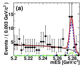
Figure 9: Left: SM Feynman diagrams for $b\to s{\cal{\ell^{+}\ell^{-}}}$. Right: Energy substituted $B$ meson mass for reconstructed $B\to K^{\ast}{\cal{\ell^{+}\ell^{-}}}$ decays. The distribution is shown for a part of the full sample with low $q^{2}$ [27].

The differential decay rate $d\Gamma/dq^{2}$, where $q^{2}$ is the invariant mass of the lepton pair, can be described in terms of effective Wilson coefficients $C_{7}^{\rm eff},~{}C_{9}^{\rm eff}$ and $C_{10}^{\rm eff}$, which include the perturbative part of the process and thus dependence on heavy masses of SM particles $m_{W},~{}m_{t}$, as well as on possible NP masses $m_{\rm NP}$. The absolute value of the coefficient $C_{7}^{\rm eff}$ can be constrained from the measured rate of $b\to s\gamma$ process, while in $b\to s{\cal{\ell^{+}\ell^{-}}}$ additional information (on sign of $C_{7}^{\rm eff}$, as well as $C_{9}^{\rm eff},~{}C_{10}^{\rm eff}$) can be obtained due to the interference of the two amplitudes shown in Fig. 9 (left). NP could change the values of the Wilson coefficients as well as add new operators causing the transition. In exclusive $B\to K^{\ast}{\cal{\ell^{+}\ell^{-}}}$ decays the theoretical description includes beside the Wilson coefficients also the non-perturbative part expressed by the form factors which are predicted with an accuracy of around 30% [26]. This uncertainty is significantly reduced in some observables arising from the study of angular distributions, like the lepton forward-backward asymmetry ($A_{FB}$) and the fraction of longitudinally polarized $K^{\ast}$’s ($F_{L}$).

BaBar performed a study of $B\to K^{\ast}{\cal{\ell^{+}\ell^{-}}}$ decays in [27]. The reconstruction proceeds through identification of a lepton pair ($\mu^{+}\mu^{-}$ or $e^{+}e^{-}$) with invariant mass not in the range of charmonium states $J/\psi$ or $\psi(2S)$. The $K^{\ast}$ can be either charged or neutral, reconstructed through $K\pi,~{}K\pi^{0}$ and $K_{S}\pi$ final states. The signal can be seen in the energy substituted $B$ meson mass, $M_{ES}=(E_{CM}/2)^{2}-(\sum_{i}\vec{p}_{i})^{2}$, where $\vec{p}_{i}$ and $E_{CM}$ are the $B$ decay products momenta and $e^{+}e^{-}$ collision energy, respectively, calculated in the CM frame (Fig. 9 (right)). The background is composed of combinatorial one (described by reconstructing events with $\mu^{\pm}e^{\mp}$ lepton pairs), hadrons misidentified as muons (in $\mu^{\pm}\mu^{\mp}$ channel) and peaking background from $B\to D\pi$ decays where the charmed meson decays to $K^{\ast}\pi$ (vetoed by requiring the invariant mass of $K^{\ast}\pi$ not to be consistent with a $D$ meson).

For the reconstructed events the distribution of the kaon helicity angle in the rest frame of $K^{\ast}$ is investigated to obtain the fraction of longitudinally polarized $K^{\ast}$’s ($F_{L}$). $F_{L}$ value is then used as an input to the fit to the distribution of the angle between the lepton and $K^{\ast}$ in the ${\cal{\ell^{+}\ell^{-}}}$ rest frame. This angle follows a $1+3F_{L}+(1-F_{L})\cos^{2}{\theta_{\cal{\ell}}}+(8/3)A_{FB}\cos{\theta_{\cal{\ell}}}$ distribution. The $A_{FB}$ is the lepton forward-backward asymmetry which can be predicted in terms of the Wilson coefficients. In Fig. 10 (left) measured $A_{FB}$ is shown as a function of $q^{2}$ for the measurement by BaBar as well as the most recent measurement by Belle collaboration [28]. The measured values are compared to the SM prediction and the expectation for the Wilson coefficient $C_{7}^{\rm eff}$ of reversed sign. In general the measurements seems to be shifted to larger asymmetry values than predicted.

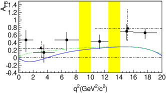
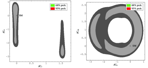
Figure 10: Left: Measured $A_{FB}$ as a function of $q^{2}$ in $B\to K^{\ast}{\cal{\ell^{+}\ell^{-}}}$ decays. The data points marked with triangles (dashed-dotted error bars) are from [27] and circular data points (full error bars) from [28]. The shaded regions represent $q^{2}$ intervals not included in the measurement ($J/\psi,~{}\psi(2S)$ regions). Full line represents the SM prediction and the dashed curve prediction with $C_{7}^{\rm eff}=-C_{7}^{\rm SM,~{}eff}$. Right: Constraints on NP contributions to Wilson coefficients arising from measurements of various FCNC processes [29]. The SM corresponds to $\delta C_{i}=0$. Light shaded areas represent the 68% C.L. and dark shaded the 95% C.L. region.

Similarly as for the $b\to s\gamma$ decays, also for $b\to s{\cal{\ell^{+}\ell^{-}}}$ semi-inclusive measurements have been performed by summing up various hadronic decay modes of the strange quark system ($K_{S}$ or $K^{\pm}$ with 0 to 4 pions) accounting for around 70% of the total decay rate. The average of the branching fraction measurements is $Br(B\to X_{s}{\cal{\ell^{+}\ell^{-}}})=(4.50\pm^{1.03}_{1.01})\times 10^{-6}$ [11].

Various measurements of FCNC can be combined to put constraints on possible NP contribution to Wilson coefficients. Within a Minimal Flavour Violation scenario these constraints are presented in Fig. 10 (right) [29]. Measurements of $Br(B\to X_{s}\gamma)$, $Br(B\to X_{s}{\cal{\ell^{+}\ell^{-}}})$, $Br(K\to\pi\nu\nu)$ and $Br(B_{s}\to\mu\mu)$ are used as the input. The combination of measurements is consistent with the SM ($\delta C_{i}=0$) although there are large areas corresponding to non-SM contributions possible.

3 Lecture II

”Charm is…a way of getting the answer yes without having to ask any clear question.” (A. Camus, 1913-1960)

3.1 $D$ meson oscillations

The second lecture is devoted to results in physics of charmed hadrons from $B$-factories. Charm physics in recent years gained in interest of both, experimental and theoretical physicists, mainly due to new interesting results from Belle and BaBar. Both experiments are not only factories of $B$ mesons but also of charmed hadrons (see Section 1 and Fig. 1). Contemporary charm physics has a twofold impact: as a ground of theory predictions tests, mainly tests of LQCD, and as a self-standing field of SM measurements and NP searches. An example of the first kind are the measurements of charmed meson decay constants, to be compared to LQCD calculations, to verify those and thus enable a more reliable estimates of the CKM matrix elements from the measurements in the $B$ meson sector. The outstanding examples of the second group of measurements are recent observations of $D^{0}$ mixing and searches for the $CP$ violation in processes involving charmed hadrons.

Neutral $D$ mesons are the only neutral meson system composed of up-like quarks. Hence a different contribution of virtual new particles than in the mixing of other neutral mesons is possible in the loops of diagrams describing the $D^{0}\leftrightarrow\bar{D}^{0}$ transition (Fig. 4 (right)). However, the short distance contribution to the mixing rate, illustrated by the box diagram, is extremely small. The reason is the effective GIM suppression; calculation of the amplitude for this transition reveals [30] that it is proportional to $V_{cs}^{\ast}V_{cd}^{\ast}V_{ud}V_{us}(m_{s}^{2}-m_{d}^{2})/m_{c}^{2}$. Hence the amplitude is doubly Cabibbo suppressed, and furthermore arises only as a consequence of SU(3) flavour symmetry breaking. The resulting oscillation frequency defined in Sect. 2.1 is $|x_{D}|={\cal{O}}(10^{-5})$. This unobservable effect is hindered by long distance contribution to the transition amplitude, for example from states accessible to both, $D^{0}$ and $\bar{D}^{0}$ (e.g. $D^{0}\to K^{+}K^{-}\to\bar{D}^{0}$). This contribution is difficult to estimate. Current calculations [31] within the SM predict $|x_{D}|,~{}|y_{D}|\lesssim{\cal{O}}(10^{-2})$. The result illustrates the order of magnitude of the mixing parameters to be expected in the $D^{0}$ system (compare to measured values of $x,~{}x_{s}$ given in Sect. 2.1) as well as the large theoretical uncertainty of the predictions.

The time evolution of an initially produced $D^{0}$ meson follows Eq. (2) with the simplification due to $|x_{D}|,~{}|y_{D}|\ll 1$:

$$\frac{d\Gamma(D^{0}\to f)}{dt}=e^{-t}|A_{f}+\frac{q}{p}\frac{ix_{D}+y_{D}}{2}A_{\bar{f}}|^{2}+{\cal{O}}(x_{D}^{3},~{}y_{D}^{3})~{}~{}.$$ (7)

The time integrated rate for an initially produced $D^{0}$ meson to decay as a $\bar{D}^{0}$, $R_{M}=(x_{D}^{2}+y_{D}^{2})/2\sim 10^{-4}$, is small and represents the reason for a 31 years time span between the discovery of $D^{0}$ mesons and the experimental observation of the $D^{0}$ mixing.

There are several methods and selection criteria common to various measurements of $D^{0}$ mixing. Tagging of the flavour of an initially produced $D^{0}$ meson is achieved by reconstruction of decays $D^{\ast+}\to D^{0}\pi_{s}^{+}$ or $D^{\ast-}\to\bar{D}^{0}\pi_{s}^{-}$. The charge of the characteristic low momentum pion $\pi_{s}$ determines the tag. The energy released in the $D^{\ast}$ decay, $q=m(D^{\ast})-m(D^{0})-m_{\pi}~{}~{}$, has a narrow peak for the signal events and thus helps in rejecting the combinatorial background. $D^{0}$ mesons produced in $B$ decays have a different decay length distribution and kinematic properties than the mesons produced in fragmentation. In order to obtain a sample of neutral mesons with uniform properties one selects $D^{\ast}$ mesons with momentum above the kinematic limit for the $B$ meson decays. The decay time is obtained from the reconstructed momentum and decay length of $D^{0}$ meson, and the latter is obtained from a common vertex of $D^{0}$ decay products and an intersection point of $D^{0}$ momentum vector and the $e^{+}e^{-}$ interaction region.

Methods of measuring the mixing parameters as well as sensitivities depend on specific final states chosen. The first to be described are decays to $CP$ eigenstate $f_{CP}$. In the limit of negligible $CP$ symmetry violation ($CPV$, described in Section 3.2) the mass eigenstates $D_{1,2}$ coincide with the $CP$ eigenstates (in case of no $CPV$ $q/p=1$, see Eq. (1)). In decays $D^{0}\to f_{CP}$ only the mass eigenstate component of $D^{0}$ with the $CP$ eigenvalue equal to the one of $f_{CP}$ contributes. By measuring the lifetime of $D^{0}$ in decays to $f_{CP}$ one thus determines the corresponding $1/\Gamma_{1}$ or $1/\Gamma_{2}$. On the other hand, flavour specific final states like $K^{-}\pi^{+}$ have a mixed $CP$ symmetry. The measured value of the effective lifetime in these decays corresponds to a mixture of $1/\Gamma_{1}$ and $1/\Gamma_{2}$. The relation between the two lifetimes can be written as [32]

$$\tau(f_{CP})=\frac{\tau(D^{0})}{1+\eta_{f}y_{CP}}~{}~{},$$ (8)

where $\tau(f_{CP})$ and $\tau(D^{0})$ are the lifetimes measured in $D^{0}\to f_{CP}$ and $D^{0}\to K^{-}\pi^{+}$, respectively. $\eta_{f}=\pm 1$ denotes the $CP$ eigenvalue of $f_{CP}$. The relative difference of the lifetimes is described by the parameter $y_{CP}$. Expressed in terms of the mixing parameters, $y_{CP}$ reads [32] $y_{CP}=y_{D}\cos{\phi}-(1/2)A_{M}x_{D}\sin{\phi}$, with $A_{M}$ and $\phi$ describing the $CPV$ in mixing and in interference between mixing and decays, respectively. In case of no $CPV$, $A_{M}=\phi=0$ and $y_{CP}=y_{D}$.

The measurement of $y_{CP}$ by Belle [33] represents the first evidence of $D^{0}$ mixing . Number of reconstructed decays to $CP$-even states $K^{+}K^{-}$ and $\pi^{+}\pi^{-}$ were $110\times 10^{3}$ and $50\times 10^{3}$, with purities of $98\%$ and $92\%$, respectively. A simultaneous fit to the decay time distributions of $KK,~{}\pi\pi$ and $K\pi$ decays was performed with $y_{CP}$ as a common free parameter. In order to perform a precision measurement of lifetime in each of the decay modes a special care should be devoted to a proper description of $t$ resolution function in various data-taking periods (for details the reader is referred to the original publication). The $t$ distributions and the result of the fit are presented in Fig. 11. The quality of the fit ($\chi^{2}/n.d.f.=313/289$) confirms an accurate description of the resolution effects.

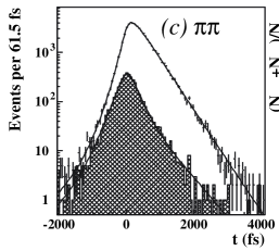
Figure 11: Decay time distributions of $D^{0}\to h^{+}h^{-}$ ($h=K,~{}\pi$) [33]. Hatched histogram is the contribution of background obtained from $m(h^{+}h^{-})$ sidebands. Full line is the result of a simultaneous fit to all three distributions with $y_{CP}$ as a common free parameter.

The measured value of $y_{CP}$ is $(1.31\pm 0.32\pm 0.25)\%$ and the largest contribution to the systematic uncertainty arises due to a possible small detector induced bias in the decay time determination. $y_{CP}$ deviates from the null value by more than three standard deviations including the systematic uncertainty. This evidence is confirmed by a similar measurement performed by the BaBar collaboration [35], finding $y_{CP}=(1.24\pm 0.30\pm 0.13)\%$.

Another possibility to look for the effect of mixing represent decays of initially produced $D^{0}$’s to a wrong-sign final state $K^{+}\pi^{-}$. While the more abundant $D^{0}$ decays lead to the $K^{-}\pi^{+}$ charge combination, the wrong-sign combination can be reached through doubly Cabibbo suppressed (DCS) decays or through a $D^{0}\to\bar{D}^{0}$ mixing followed by a Cabibbo favored (CF) $\bar{D}^{0}$ decay. In order to separate the mixing contribution from the DCS decays an analysis of the decay time distribution must be performed. The $t$-dependent decay rate, $d\Gamma(D^{0}\to K^{+}\pi^{-})\propto[R_{D}+\sqrt{R_{D}}y_{D}^{\prime}t+(1/4)(x_{D}^{\prime 2}+y_{D}^{\prime 2})t^{2}]e^{-t}$, consists of three terms corresponding to DCS term ($R_{D}$), mixing term ($x_{D}^{\prime 2}+y_{D}^{\prime 2}$) and the interference between the two. Additional complication in the interpretation of the result arises since the decay rate depends on parameters $x^{\prime}$ and $y^{\prime}$ which are the mixing parameters rotated by a strong phase difference between the amplitudes of CF and DCS decays. In [34] BaBar collaboration fitted the $t$ distribution of around 4000 reconstructed wrong-sign decays. Result of the fit is presented in Fig. 12 (left) in terms of the allowed region in $(x^{\prime 2},y^{\prime})$ plane. While the central value is in the physically forbidden region ($x^{\prime 2}<0$) the no-mixing point ($(x^{\prime 2},y^{\prime})=(0,0)$) is excluded by a confidence level corresponding to 3.9 standard deviations.

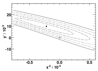
Figure 12: Left: Likelihood contours in $(x^{\prime 2},y^{\prime})$ plane arising from the measurement of $D^{0}\to K^{+}\pi^{-}$ decays [34]. The lines correspond to 1-5 $\sigma$ C.L., the dot represents the central value and the cross the no-mixing point. Right: 95% C.L. contour of $(x_{D},y_{D})$ as determined in the time-dependent Dalitz study of $D^{0}\to K_{S}\pi^{+}\pi^{-}$ [36]. Regions arising from the fit with neglected and allowed $CPV$, as well as neglecting or incorporating the systematic uncertainty are shown.

Numerically they find $x^{\prime 2}=(-0.22\pm 0.33\pm 0.21)\times 10^{-3}$ and $y^{\prime}=(0.97\pm 0.44\pm 0.31)\%$.

The method which allows for a direct determination of both mixing parameters, $x_{D}$ and $y_{D}$, is the study of decays into self conjugated multi-body final states. Several intermediate resonances can contribute to such a final state. In the recent measurement by Belle [36] the $K_{S}\pi^{+}\pi^{-}$ final state was analyzed, where contributions from CF decays (e.g. $D^{0}\to K^{\ast-}\pi^{+}$), DCS decays (e.g. $D^{0}\to K^{\ast+}\pi^{-}$) and decays to $CP$ eigenstates (e.g. $D^{0}\to\rho^{0}K_{S}$) are present. Individual contributions can be identified by analyzing the Dalitz distribution of the decay. Due to the interference among different types of decays it is possible to determine their relative phases (unlike in $D^{0}\to K^{+}\pi^{-}$ decays where the relative phase between DCS and CF decays cannot be determined). And most importantly, since these types of intermediate states also exhibit a specific time evolution one can determine directly the mixing parameters $x_{D}$ and $y_{D}$ by studying the time evolution of the Dalitz distribution. The signal p.d.f. for a simultaneous fit to the Dalitz and decay-time distribution is

$$|\langle K_{S}\pi^{+}\pi^{-}|D^{0}(t)\rangle|^{2}=|\frac{1}{2}{\cal{A}}(m_{-}^{2},m_{+}^{2})\bigl{[}e^{-i\lambda_{1}t}+e^{-i\lambda_{2}t}\bigr{]}+\frac{1}{2}\overline{\cal{A}}(m_{-}^{2},m_{+}^{2})\bigl{[}e^{-i\lambda_{1}t}-e^{-i\lambda_{2}t}\bigr{]}|^{2}~{}~{},$$ (9)

composed of an instantaneous amplitude for $D^{0}$ decay, ${\cal{A}}(m_{-}^{2},m_{+}^{2})$, and an amplitude for the $\bar{D}^{0}$ decay, $\bar{\cal{A}}(m_{-}^{2},m_{+}^{2})$, arising due to a possibility of mixing. They both depend on the Dalitz variables $m_{-}^{2}=m^{2}(K_{S}\pi^{-})$ and $m_{+}^{2}=m^{2}(K_{S}\pi^{+})$. The dependence on the mixing parameters is hidden in $\lambda_{1,2}=m_{1,2}-i\Gamma_{1,2}/2$. If $CPV$ is neglected the amplitude for $\bar{D}^{0}$ tagged decays is $|\langle K_{S}\pi^{+}\pi^{-}|\bar{D}^{0}(t)\rangle|^{2}(m_{+}^{2},m_{-}^{2},t)=|\langle K_{S}\pi^{+}\pi^{-}|D^{0}(t)\rangle|^{2}(m_{-}^{2},m_{+}^{2},t)$. As in the case of $B^{0}$ oscillation measurements the p.d.f. of Eq. (9) must be corrected to include the finite resolution on the decay time.

Based on $\sim 500\times 10^{3}$ reconstructed decays with a purity of 95% Belle obtained a good description of the Dalitz distribution using 18 different resonant intermediate states and a non-resonant contribution. A simultaneous fit to $m_{-}^{2},~{}m_{+}^{2}$ and $t$ yielded mixing parameters $x_{D}=(0.80\pm 0.29\pm^{0.13}_{0.16})\%$, $y_{D}=(0.33\pm 0.24\pm^{0.10}_{0.14})\%$. This represents by far the most constraining determination of $x_{D}$ up to date. Contour of allowed $(x_{D},y_{D})$ values at 95% C.L. is shown in Fig. 12 (right).

3.2 $CP$ violation in the system of neutral $D$ mesons

A general, easy to reach expectation is that possible $CPV$ in processes involving charmed hadrons must be small within the SM. This arises due to the fact that such processes involve the first two generations of quarks for which the elements of the CKM matrix are almost completely real. Typical CKM factor entering both the short distance box diagram as well as the decays to real states accessible to both, $D^{0}$ and $\bar{D}^{0}$, is $V_{cs}^{\ast}V_{us}$. Using CKM matrix unitarity this can be expressed as $-V_{cd}^{\ast}V_{ud}[1+(V_{cb}^{\ast}V_{ub})/(V_{cd}^{\ast}V_{ud})]$. Considering the small absolute value of the second term one can see that $\arg(V_{cs}^{\ast}V_{us})\approx\Im((V_{cb}^{\ast}V_{ub})/(V_{cd}^{\ast}V_{ud}))\sim 7\times 10^{-4}$. This is the typical value of the weak phase in charmed hadron processes which determines the size of the $CPV$ effects in the SM. For example, $CPV$ asymmetries like $A_{\Gamma}$ discussed below, are typically of the order of $x_{D}\sin\phi$, where $\phi$ is the weak phase considered, and hence $A_{\Gamma}\sim{\cal{O}}(10^{-5})$. Deviation of $|q/p|$ value from unity, which also represents the $CP$ violation, is roughly expected to be of the order of $\sin\phi\sim 10^{-3}$. These values are all below the current experimental sensitivity and any positive experimental signature would be a clear sign of some contribution beyond the SM.

All three distinct types of $CP$ violation, $CPV$ in decays, in mixing and in the interference between decays with and without mixing (see lectures by A.J. Bevan) can in principle be present in the $D^{0}$ system. They are parameterized by $A_{D}$, $A_{M}$ and $\phi$ according to

$$\frac{A_{f}}{\bar{A}_{\bar{f}}}=1+\frac{A_{D}}{2};~{}~{}(A_{D}\neq 0,~{}CPV~{}{\rm in~{}decay})$$

$$|\frac{q}{p}|=1+\frac{A_{M}}{2};~{}~{}(A_{M}\neq 0,~{}CPV~{}{\rm in~{}mixing})$$

$$\frac{q}{p}\frac{\bar{A}_{f}}{A_{f}}=-\frac{(1+A_{M}/2)\sqrt{R_{D}}}{1+A_{D}/2}e^{i(\phi-\delta_{f})};~{}~{}(\phi\neq 0,~{}CPV~{}{\rm in~{}interference})~{}~{}.$$ (10)

In the above equations $\sqrt{R_{D}}$ is the ratio of amplitude magnitudes $|\bar{A}_{f}/A_{f}|$ and $\delta_{f}$ is the strong phase difference between the two.

In all mentioned mixing parameter measurements also a search for possible $CPV$ has been performed .

In decays to $CP$ eigenstates ($D^{0}\to KK,~{}\pi\pi$) one measures lifetimes separately for $D^{0}$ and $\bar{D}^{0}$ tagged events. A measurable asymmetry

$$A_{\Gamma}=\frac{\tau(\bar{D}^{0}\to f_{CP})-\tau(D^{0}\to f_{CP})}{\tau(\bar{D}^{0}\to f_{CP})+\tau(D^{0}\to f_{CP})}$$ (11)

is related to the mixing and $CPV$ parameters as [32] $A_{\Gamma}=(1/2)A_{M}y_{D}\cos\phi-x_{D}\sin\phi$ and equals zero in the case of no $CPV$. The measured values by Belle [33] and Babar [35] are $A_{\Gamma}=(0.01\pm 0.30\pm 0.15)\%$ and $A_{\Gamma}=(0.26\pm 0.36\pm 0.08)\%$, respectively. Hence there is no sign of the $CP$ violation at the sensitivity level of around 0.3%.

In $D^{0}\to K^{+}\pi^{-}$ decays the decay time distribution is also fitted separately for $D^{0}$ mesons and their anti-particles. There are six observables, $x^{\prime\pm},~{}y^{\prime\pm},~{}R_{D}^{\pm}$, where the $\pm$ superscripts denote the observables for $D^{0}$ and $\bar{D}^{0}$ subsamples. They are related to the parameters of Eq. (10) by $A_{D}=(R_{D}^{+}-R_{D}^{-})/(R_{D}^{+}+R_{D}^{-})$, $R_{M}^{\pm}=(x^{\prime\pm 2}+y^{\prime\pm 2})/2$ and $A_{M}=(R_{M}^{+}-R_{M}^{-})/(R_{M}^{+}+R_{M}^{-})$. From such fits the results of the search for $CPV$ in mixing and in decay are $A_{M}=0.1\pm 2.9,~{}A_{D}=(-2.1\pm 5.4)\%$ [34] or $A_{M}=0.67\pm 1.2,~{}A_{D}=(-2.3\pm 4.7)\%$ [39] (errors here include statistical and systematic uncertainties). There is no hint of a direct $CPV$ at the level of 5%.

In the $t$-dependent analysis of $D^{0}\to K_{S}\pi\pi$ Dalitz distribution the possibility of $CPV$ is included by additional two free parameters in the fit, $A_{M}$ and $\phi$. Also the direct $CPV$ can be checked by allowing the contributions of various intermediate states to be different for $D^{0}$ and $\bar{D}^{0}$ Dalitz distributions. The latter was not observed within the statistical uncertainties. Parameters of $CPV$ in mixing and interference are found to be $A_{M}=-0.26\pm 0.60\pm 0.20$ and $\phi=(-0.24\pm 0.31\pm 0.09)~{}rad$. The contours of $(x_{D},y_{D})$ arising from the fit allowing for the $CPV$ are presented in Fig. 12 (right).

3.3 Average of $D^{0}$ mixing parameters

To make conclusions arising from a variety of results on $D^{0}$ mixing and $CPV$ searches the Heavy Flavour Averaging Group performs an average of various measurements including correlations among the measured variables [11]. An illustration of $(x_{D},y_{D})$ constraints imposed by individual measurements is shown in Fig. 13 (left). World average of mixing and $CPV$ parameters for the $D^{0}$ system is presented in Tab. 1.

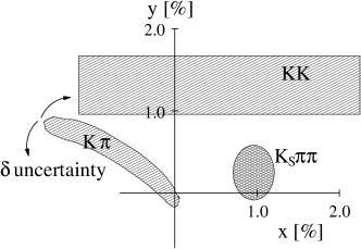
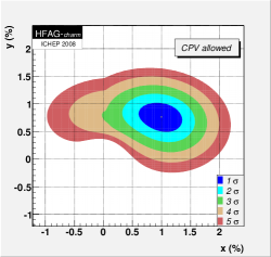
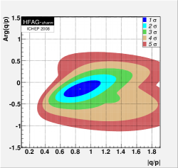
Figure 13: Left: Illustration of constraints on $(x_{D},y_{D})$ values arising from various measurements. Middle: Probability contours for $(x_{D},y_{D})$ corresponding to 1-5 $\sigma$ C.L. from the average of measurements [11]. Right: Probability contours for $CPV$ parameters $(|q/p|,\phi)$ corresponding to 1-5 $\sigma$ C.L. from the average of measurements [11].

Parameter Value Parameter Value $x_{D}$ $(1.00\pm^{0.24}_{0.26})\%$ $A_{D}$ $(-2.1\pm 2.4)\%$ $y_{D}$ $(0.76\pm^{0.17}_{0.18})\%$ $|q/p|$ $0.86\pm^{0.17}_{0.15}$ $R_{D}$ $(0.336\pm 0.009)\%$ $\phi$ $-8.8^{\circ}\pm^{7.6^{\circ}}_{7.2^{\circ}}$

Table 1: Average of $D^{0}$ mixing (left) and $CPV$ (right) parameters [11].

The results are presented graphically in Figs. 13 (middle) and 13 (right) as contours in $(x_{D},y_{D})$ and $(|q/p|,\phi)$ planes. The mixing phenomena in the neutral $D$ meson system is firmly established, with the mixing parameters $x_{D}$ and $y_{D}$ of the order of 1%. The oscillation frequency can be compared to the values for other neutral meson systems, $x\approx 0.8~{}(B^{0})$, $x_{K}\approx 1~{}(K^{0})$ and $x_{s}\approx 25~{}(B_{s}^{0})$. Since both parameters, $x_{D}$ and $y_{D}$, appear to be positive, it seems that the $CP$-even state of neutral charmed mesons is shorter-lived (like in the $K^{0}$ system) and also heavier (unlike in the $K^{0}$ system). At the moment there is no sign of $CPV$ in the $D^{0}$ system, at the level of one standard deviation of the world average results.

Results in the $D^{0}$ mixing impose some stringent constraints on the parameters of various NP models [40]. As an example we quote the $R$-parity violating Supersymmetry models, where an enhancement of $x_{D}$ could arise from an exchange of down-like squarks or sleptons in the loop of the box diagram. The exclusion region of possible values of the squark mass and $R$-parity violating coupling constants for various upper limits on $x_{D}$ is presented in Fig. 14 (left).

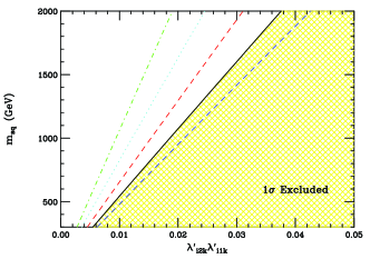
Figure 14: Left: Constraints on the values of squark mass and $R$-parity violating coupling constants arising from $x_{D}<1\%$ (hatched region is excluded). Dashed lines represent boundaries of the exclusion region for $x_{D}<1.5\%,~{}0.8\%,~{}0.5\%$ and $0.3\%$ [40]. Right: Sketch of a method to measure $Br(D_{s}^{+}\to\mu^{+}\nu)$ [41]. Full lines represent particles detected in the detector or exclusively reconstructed, and dashed lines particles reconstructed in the recoil (from the known momenta of incident beams and detected particles).

Planned Super $B$-factory, which would accumulate data corresponding to an integrated luminosity of 50 ab^-1 (compared to the current 0.8 ab^-1 at KEKB), would of course yield results on $D^{0}$ mixing and $CPV$ of much better precision. The extrapolated accuracies are $\sigma(x_{D})\sim 0.1\%,~{}\sigma(y_{D})\sim 0.06\%,~{}\sigma(|q/p|)\sim 0.05$ and $\sigma(\phi)\sim 3^{\circ}$. This would allow to severely constrain relations among parameters of various NP parameters and to search for possible $CPV$ phenomena in the region where a large number of these models predict an observable effect. However, one should not forget the words ”Prediction is very difficult, especially of the future.” (N. Bohr, 1885 - 1962).

3.4 $D_{s}$ leptonic decays

Charmed mesons leptonic decays are analogous to the leptonic decays of $B$ mesons (Sect. 2.2). By measuring the rate of such decays one would hope to determine the decay constant of the corresponding meson, see Eq. (6), and by that test the predictions of LQCD. Both Belle and BaBar performed measurements of $Br(D_{s}^{+}\to\mu^{+}\nu)$. Cleo-c collaboration measured decays $D_{s}^{+}\to\tau\nu$ as well.

In [41] Belle measured the absolute branching fraction of $D_{s}^{+}\to\mu^{+}\nu$ using a method illustrated in Fig. 14 (right). Events of the type $e^{+}e^{-}\to D_{s}^{\ast}D^{\pm,0}K^{\pm,0}X$ are used, where $X$ can be any number of additional pions from fragmentation, and up to one photon. An event is divided into a tag side, where a full reconstruction of $D$ and a primary $K$ meson is performed, and a signal side where the decay chain $D_{s}^{\ast+}\to D_{s}^{+}\gamma$, $D_{s}^{+}\to\mu^{+}\nu_{\mu}$ is searched for. Tag side charged and neutral $D$ mesons are reconstructed in $D\to Kn\pi$ decays. For all possible combinations of particles in $X$, the signal side $D_{s}^{\ast+}$ meson is identified by reconstruction of the recoil mass $m_{\rm rec}(DKX)$, using the known beam momentum and four-momentum conservation. The recoil mass $m_{\rm rec}(Y)$ is calculated as the magnitude of the four-momentum $p_{\rm beams}-p_{Y}$. The next step in the event reconstruction is a search for a photon for which the recoil mass $m_{\rm rec}(DKX\gamma)$ is consistent with the nominal mass of $D_{s}^{+}$. The sample of $D_{s}^{+}$ mesons reconstructed using this procedure represent an inclusive sample of decays, among which the leptonic decays are searched for. If an identified muon is found among the tracks so far not used in the reconstruction, the square of the recoil mass $m^{2}_{\rm rec}(DKX\gamma\mu)$ is calculated. For signal decays this mass corresponds to the mass of the final state neutrino and hence peaks at zero.

Final distribution of $m^{2}_{\rm rec}(DKX\gamma\mu)$ is shown in Fig. 15 (left) where a clear signal of leptonic decays can be seen. Majority of background can be described using reconstructed $D_{s}^{+}\to e^{+}\nu$ decays where due to the helicity suppression no signal is expected. Number of reconstructed signal decays is found to be $N(D_{s}^{+}\to\mu^{+}\nu)=169\pm 16\pm 8$. Comparing to the number of inclusively reconstructed $D_{s}^{+}$ decays and correcting for the efficiency of muon reconstruction one obtains the branching fraction $Br(D_{s}^{+}\to\mu^{+}\nu)=(6.44\pm 0.76\pm 0.56)\times 10^{-3}$. The largest contribution to the systematic uncertainty arises from a limited number of simulated decays used to describe the shape of the signal distribution. Using Eq. (6) (without the factor arising from the charged Higgs contribution) and the value of $|V_{cs}|$ as determined in a global fit to the CKM elements applying the unitarity of the matrix [9], one determines the value of $D_{s}$ meson decay constant, $f_{D_{s}}=(275\pm 16\pm 12)$ MeV.

BaBar [42] used a somewhat different approach by measuring the yield of $D_{s}^{+}\to\mu^{+}\nu$ relative to the $D_{s}^{+}\to\phi\pi$ decays. The branching fraction determined in this way is a relative measurement normalized to the $Br(D_{s}^{+}\to\phi\pi)$. While this method enables a larger statistics of the reconstructed sample it suffers from a hard-to-estimate systematic uncertainty in the normalization mode ($\phi\pi$ state is actually an intermediate state of the $K^{+}K^{-}\pi^{+}$ final state and can be influenced by the interference among various intermediate states). The neutrino momentum is determined from the missing momentum in an event. The resolution is improved by constraining the $\nu$ and the reconstructed muon momentum to yield the nominal mass of $D_{s}$ meson. Fig. 15 (right) shows the distribution of the reconstructed mass difference between the $D_{s}^{\ast}$ and $D_{s}$ meson, where the signal of leptonic decays consist of $489\pm 55$ events (the error is statistical only). Calculation of the decay constant yields a value of $f_{D_{s}}=(283\pm 17\pm 7\pm 14)$ MeV, where the last error is due to the uncertainty of $Br(D_{s}^{+}\to\phi\pi)$.

How do the measured values compare to the LQCD calculations? The average of absolute measurements (beside the described Belle measurement these include measurements by Cleo-c collaboration in muon and tau decay modes [44]) is $f_{D_{s}}=(274\pm 10)$ MeV [20]. The recent LQCD result exhibits a huge improvement in the accuracy compared to previous determinations of the $D_{s}$ meson decay constant: $f_{D_{s}}=(241\pm 3)$ MeV [43]. The discrepancy between the two values is more than 3 standard deviations. While the fact that for the $D^{+}$ decay constant experimental results confirm the calculation (albeit within larger errors) may point to some intervention of NP [45] one should probably wait for a) confirmation of the LQCD estimate (and especially its uncertainty) and b) more accurate experimental measurements before making any conclusion .

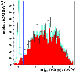
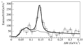
Figure 15: Left: Distribution of $m^{2}_{\rm rec}(DKX\gamma\mu)$ for $D_{s}^{+}\to\mu^{+}\nu$ candidate events [41]. The peak at zero corresponds to the signal decays. Right: $m(D_{s}^{\ast})-m(D_{s})$ distribution for $D_{s}^{+}\to\mu^{+}\nu$ candidate events [42]. Signal peaks at the nominal mass difference.

4 Summary

Although in the lectures we were able to present only a small fraction of exciting physics results that arose from the $B$-factories over almost a decade of operation, we hope the selected examples demonstrate the following:

• $B$-factories have successfully performed precision measurements in identification of SM processes and determination of SM parameters, as well as a complement to direct NP searches that are soon to be started at the LHC;

• experimental tests in general confirm predictions of the SM, although several hints of discrepancies at the level of 3 standard deviations exist;

• $B$-factories have outreached their program as foreseen at the startup.

Specifically related to the presented measurements one should note

• $B$ oscillations in conjunction with a breakthrough in $B_{s}$ oscillations confirm the SM to a high accuracy;

• leptonic and radiative $B$ meson decays constrain possible contribution of NP but large room for improvement remains for the Super $B$-factory;

• important results in charm physics complement the results in the $B$ meson sector;

• measurements of $D^{0}$ mixing and search for the $CPV$ represent another achieved milestone in particle physics, more precise measurements and theoretical predictions are needed;

• $D_{s}$ leptonic decays may test predictions of LQCD once the results are confirmed.

4.1 Acknowledgments

The author wishes to thank the organizers of the school for the great summer school atmosphere and a very pleasant stay in Dubna. Most of the measurements presented in the lectures are the result of a splendid work of the Belle and BaBar collaboration members and of the superb performance of the KEKB and PEP-II accelerators.

The credit for the quotes used goes to:
Oscar Wilde, Irish playwright, poet, 1854-1900.
Anne Frank, Jewish girl, author of the famous diary, 1929-1945.
Ralph Waldo Emerson, American Poet and Essayist, 1803-1882.
Sir Sean Connery, Scottish actor and producer, 1930.
Albert Camus, Algerian-born French writer, 1913-1960.
Niels Bohr, Danish physicist, 1885-1962.

References

- [1] A. Bevan, arXiv:0812.4388.
- [2] A. Abashian et al. (Belle Coll.), Nucl. Instr. Meth. A479, 117 (2002).
- [3] S. Kurokawa, E. Kikutani, Nucl. Instr. Meth. A499, 1 (2003), and other papers in this volume.
- [4] B. Aubert et al. (BaBar Coll.), Nucl. Instr. Meth. A479, 1 (2002).
- [5] D. Acosta et al. (CDF Coll.), Phys. Rev. D71, 032001 (2005).
- [6] D. Peterson et al., Nucl. Instr. Meth. A478, 142 (2002); Y. Kubota et al. (CLEO Coll.), Nucl. Instr. Meth. A320, 66 (1992).
- [7] D. Kirkby, Y. Nir, review CP Violation in Meson Decays, in C. Amsler et al., Phys. Lett. B667, 1 (2008), and references therein.
- [8] H. Tajima et al., Nucl. Instr. Meth. A533, 370 (2004).
- [9] C. Amsler et al., Phys. Lett. B667, 1 (2008).
- [10] K. Abe et al. (Belle Coll.), Phys. Rev. D71, 072003 (2005).
- [11] E. Barberio et al. (HFAG), arXiv:0808.1297, and updates at http://www.slac.stanford.edu/xorg/hfag/
- [12] A.J. Buras et al., Nucl. Phys. B245, 369 (1984).
- [13] J. Charles et al. (CKMfitter group), Eur. Phys. J. C41, 1 (2005).
- [14] http://ckmfitter.in2p3.fr
- [15] A. Abulencia et al. (CDF Coll.), Phys. Rev. Lett. 97, 242003 (2006).
- [16] I. Adachi et al. (Belle Coll.), arXiv:0809.3834.
- [17] B. Aubert et al. (BaBar Coll.), Phys. Rev. D76, 052002 (2007).
- [18] K. Ikado et al. (Belle Coll.), Phys. Rev. Lett. 97, 251802 (2006).
- [19] M. Artuso, E. Barberio, S. Stone, arXiv:0902:3743.
- [20] See J. Rosner, S. Stone, review Decay Constants of Charged Pseudoscalar Mesons, in C. Amsler et al., Phys. Lett. B667, 1 (2008), and references therein.
- [21] A. Gray et al. (HPQCD Coll.), Phys. Rev. Lett. 95, 212001 (2005).
- [22] K. Abe et al. (Belle Coll.), arXiv:0804.1580.
- [23] B. Aubert et al. (BaBar Coll.), Phys. Rev. D72, 052004 (2005).
- [24] M. Misiak et al., Phys. Rev. Lett. 98, 022002 (2007).
- [25] U. Egede et al., arXiv:0807.2589, and references therein.
- [26] A. Ali et al., Phys. rev. D66, 034002 (2002).
- [27] B. Aubert et al. (BaBar Coll.), arXiv:0804.4412.
- [28] I. Adachi et al. (Belle Coll.), arXiv:0810.0335.
- [29] T. Hurth et al., arXiv:0807.5039.
- [30] G. Burdman, I. Shipsey, Ann. Rev. Nucl. Sci. 53, 431 (2005).
- [31] I.I. Bigi, N. Uraltsev, Nucl. Phys. B592, 92 (2001); A.F. Falk et al., Phys. Rev. D69, 114021 (2004).
- [32] S. Bergmann et al., Phys. Lett. B 486, 418 (2000).
- [33] M. Starič et al. (Belle Coll.), Phys. Rev. Lett. 98, 211803 (2007).
- [34] B. Aubert et al. (BaBar Coll.), Phys. Rev. Lett. 98, 211802 (2007).
- [35] B. Aubert et al. (BaBar Coll.), Phys. Rev. D78, 011105 (2008).
- [36] L.M. Zhang et al. (Belle Coll.), Phys. Rev. Lett. 99, 131803 (2007).
- [37] U. Bitenc et al. (Belle Coll.), Phys. Rev. D77, 112003 (2008).
- [38] B. Aubert et al. (BaBar Coll.), Phys. Rev. Lett. 100, 061803 (2008).
- [39] L.M. Zhang et al. (Belle Coll.), Phys. Rev. Lett. 96, 151801 (2006).
- [40] E. Golowich et al., Phys. Rev. D76, 095009 (2007).
- [41] L. Widhalm et al. (Belle Coll.), Phys. Rev. Lett. 100, 241801 (2008).
- [42] B. Aubert et al. (BaBar Coll.), Phys. Rev. Lett. 98, 141801 (2007).
- [43] E. Follana et al. (HPQCD and UKQCD Coll.), Phys. Rev. Lett. 100, 062002 (2008).
- [44] M. Artuso et al. (Cleo-c Coll.), Phys. Rev. Lett. 99, 071802 (2007); K.M. Ecklund et al. (Cleo-c Coll.), Phys. Rev. Lett. 100, 161801 (2008).
- [45] B.A. Dobrescu, A.S. Kronfeld, Phys. Rev. Lett. 100, 241802 (2008).
- [46] W.S. Hou, Phys. Rev. D48, 2342 (1993).