Cosmic Duality and Statefinder Diagnosis of Spinor Quintom

Abstract

In this paper, we study the possible connections among different Spinor Quintom Dark Energy (DE) models by the aid of duality. Then we apply the statefinder diagnostic to these models. By this diagnostic pair $\{r,s\}$, we differentiate one Quintom DE model from the others in a model independent manner. A class of evolutionary trajectories of these Spinor Quintom models are presented in the statefinder parameter planes. We also obtain the current locations of the parameters $r$ and $s$, and these locations correspond to different models in statefinder parameter planes theoretically.

I Introduction

There are mounting data from type Ia supernovae and cosmic microwave background (CMB) radiation and so on [1, 2, 3, 4]. All these data have provided strong evidences for the present universe, which is spatially flat, accelerated expanding and dominated by dark sectors. The combined analysis of the above cosmological observations supports that the contents of the universe comprise about $73\%$ DE, $23\%$ cold dark matter (CDM), and only $4\%$ usual baryon matter which can be described by the well-known particle theory. In terms of Friedmann-Robertson-Walker (FRW) cosmology, this acceleration is attributed to an exotic form with negative pressure, the so-called DE. So far, the nature of DE remains a mystery. Theoretically, the obvious candidate for such a component is a small cosmological constant $\Lambda$ (or vacuum energy) with Equation of State (EoS) $w=-1$. The corresponding cosmological model — LCDM (or $\Lambda$CDM) — consists of a mixture of vacuum energy and CDM, but there exsits the fine tuning and the coincidence problems. The inspiration of inflation suggests that DE is attributed to the dynamics of a scalar field or multi-scalar fields, such as the Quintessence [5, 6], Phantom [7], K-essence [8, 9, 10]. There are also other DE models such as Chaplygin gas [11], Braneworld models [12, 13], Holographic models [14, 15, 16, 17], and so on. Although the recent fits to the data from combination of WMAP [18, 19], the recently released 182 SNIa Gold sample [20] and also other cosmological observational data show remarkably consistence of the cosmological constant, it is worth noting that a class of dynamical models with EoS across $-1$ Quintom is mildly favored [21, 22, 23, 24]. In the literature there have been a lot on theoretical studies of Quintom-like models [25, 26, 27, 28, 29, 30, 31, 32, 33, 34, 35, 36, 37, 38, 39, 40, 42, 41].

Previously, it has been proved that a Quintom DE model and its combination with Chaplygin gas fluid can be realized by non-regular spinor matter [43]. Interestingly, this type of model can realize many kinds of Quintom scenarios by transforming the form of potential of the spinor. Two typical Quintom models among these are Quintom-A and Quintom-B: the former with EoS $w>1$ at early time and $w<1$ lately; while the latter with the EoS arranged and changing from below $-1$ to above $-1$. To understand the possible combinations among different types of Quintom model in spinor field, we perform the implications of cosmic duality in this class of models in this paper. Cosmic duality is a mathematic feature which originates from string cosmology [44, 45]. Later on, cosmic duality is used to connect the standard cosmology with phantom cosmology and generalized into studies in more complicated DE models (see Refs. [46, 47, 48, 49]). Ref. [34] was pointed out that there is a dual behavior between the models of Quintom-A and Quintom-B. By studying the behavior of the energy density and pressure in spinor field, we find a duality between the Quintom-A and Quintom-B. Meanwhile, we realize other Quintom models by considering this property.

Since more and more DE models have been developed to explain the current cosmic acceleration, a method for discriminating contenders in a model independent manner was proposed by Sahni in Ref. [50, 51]. The new cosmological diagnostic pair $\{r,s\}$, called statefinder, is a geometrical diagnostics. This diagnostics is algebraically related to the higher derivatives of the scale factor $a$ with respect to time. It seems a natural next step to study beyond the Hubble parameter $H\equiv\frac{\dot{a}}{a}$ and the deceleration parameter $q$. Because the model-dependent physical variables describing the DE depend on the properties of physical fields, the DE models can be distinguished more effectively by statefinder than these variables. Hitherto, some DE models have been perfectly differentiated, such as LCDM universe, Quintessence, Phantom, the Chaplygin gas, Braneworld models, Holographic models, and interacting and coupling DE models. Correlative work has been performed by Ref. [52, 53, 54, 55, 56, 57, 58, 59, 60, 61, 62, 63, 64, 65]. We apply diagnostic to the Spinor Quintom models and present the trajectories in the $r-s$ plane corresponding to these kinds of Quintom DE models. The fixed point $\{r,s\}=\{1,0\}$ is in correspondence with the spatially flat LCDM scenario. For one given Quintom model in spinor field, the departure from the fixed point $\{r,s\}=\{1,0\}$ provides a nice way to determine the distance from LCDM.

This paper is organized as follows: In section 2, we realize possible connections among the different spinor Quintom DE models using the cosmic duality. In section 3, we apply the statefinder diagnostic to these Spinor Quintom DE models. Section 4 gives discussions and conclusions.

II Duality of Spinor Quintom Universes

In this section, we investigate the possible connections among different Spinor Quintom models and realize more Quintom DE models by the aid of the cosmic duality. The cosmic duality has been investigated by many work. The authors of Ref.[66, 67, 68] have considered a possible transformation with the Hubble parameter and studied the relevant issues with the cosmic duality[44, 45]. Specifically, Ref.[46] has shown a connection between a quintessence cosmology and a contracting phantom cosmology. Later on, this duality has been generalized into studies with more complicated DE models[47, 48, 69, 70]. Moveover, The form invariance transformations are used to constructed phantom cosmology and extended to the fermion fields [71]. Motivated by these work, we investigate the cosmic duality in the Spinor Quintom scenario under the transformation performed in Ref. [66, 67, 68].

We consider a universe filled with Quintom DE perfect fluid in spinor field [72, 73, 74], neglecting the contributions to the components of matter and radiation. We deal with the homogeneous and isotropic FRW space-time, and assume the space-time metric as,

$$ds^{2}=dt^{2}-a^{2}(t)d\vec{x}^{2}~{}.$$ (1)

According to the dynamics of a spinor field which is minimally coupled to Einstein’s gravity[75, 76, 77], we can write down the following Dirac action in a curved background space-time

$$S_{\psi} = \int d^{4}x~{}e~{}[\frac{i}{2}(\bar{\psi}\Gamma^{\mu}D_{\mu}\psi-D_{\mu}\bar{\psi}\Gamma^{\mu}\psi)-V]$$ (2)

$$= \int d^{4}x~{}e~{}{\cal L}_{\psi}~{},$$

where, $e$ is the determinant of the vierbein $e_{\mu}^{a}$ and $V$ stands for any scalar function of $\psi$, $\bar{\psi}$ and possibly additional matter fields. We assume that $V$ only depends on the scalar bilinear $\bar{\psi}\psi$. For a gauge-transformed homogeneous and a space-independent spinor field, the equation of motion for spinor reads,

$$\dot{\psi}+\frac{3}{2}H\psi+i\gamma^{0}V^{\prime}\psi = 0~{},$$ (3)

$$\dot{\bar{\psi}}+\frac{3}{2}H\bar{\psi}-i\gamma^{0}V^{\prime}\bar{\psi} = 0~{},$$ (4)

where a dot denotes a time derivative and a prime is a derivative with respect to $\bar{\psi}\psi$, while H is Hubble parameter. Taking a further derivative, we can obtain the solution of equation of motion:

$$\bar{\psi}\psi=\frac{N}{a^{3}}~{},$$ (5)

where $N$ is a positive time-independent constant and we define it as the present value of $\bar{\psi}\psi$. From the expression of the energy-momentum tensor in Ref. [43] and the equation of motion for spinor, we get the energy density and the pressure of the spinor field:

$$\rho_{\psi} = T_{0}^{0}=V~{},$$ (6)

$$p_{\psi} = -T_{i}^{i}=V^{\prime}\bar{\psi}\psi-V~{}.$$ (7)

The EoS of the spinor field, defined as the ratio of its pressure to energy density, is given by

$$w_{\psi}\equiv\frac{p_{\psi}}{\rho_{\psi}}=-1+\frac{V^{\prime}\bar{\psi}\psi}{V}~{}.$$ (8)

To keep the energy density positive, one may see that there are $w_{\psi}>-1$ when $V^{\prime}>0$ and $w_{\psi}<-1$ when $V^{\prime}<0$ from Eq. (8). The former corresponds to a Quintessence-like phase and the latter stands for a Phantom-like phase. Therefore it requires that the derivative of the potential $V^{\prime}$ change its sign if one expects a Quintom picture. In terms of the variations of $V^{\prime}$, (1). if $V^{\prime}>0~{}~{}~{}\rightarrow~{}~{}~{}V^{\prime}<0$, we get a Quintom-A scenario which evolves from a Quintessence-like phase with $w_{\psi}>-1$ to a Phantom-like phase with $w_{\psi}<-1$; (2). while $V^{\prime}<0~{}~{}~{}\rightarrow~{}~{}~{}V^{\prime}>0$, one can obtain a Quintom-B scenario, and for which the EoS is arranged to and changes from below $-1$ to above $-1$.

In the framework of FRW cosmology, the Friedmann equation reads,

$$H^{2}=\frac{1}{3}\rho~{},$$ (9)

where we use units $8\pi G=\hbar=c=1$ and all parameters are normalized by $M_{p}=1/\sqrt{8\pi G}$ in the paper.

The form-invariant transformation [66, 67, 68] reads,

$$\bar{\rho} = \bar{\rho}(\rho)~{},$$ (10)

$$\bar{H} = -(\frac{\bar{\rho}}{\rho})^{\frac{1}{2}}H~{}.$$ (11)

Then the corresponding changes for the pressure $p$ and the EoS $w$ are,

$$\bar{p} = -\bar{\rho}-(\frac{\bar{\rho}}{\rho})^{\frac{1}{2}}(\rho+p)\frac{d\bar{\rho}}{d\rho}~{},$$ (12)

$$\bar{w} = -1-(\frac{\bar{\rho}}{\rho})^{\frac{3}{2}}\frac{d\bar{\rho}}{d\rho}(1+w).$$ (13)

Taking $\bar{\rho}=\rho$ in Eqs. (12) and (13) as an example of detailed discussion, regardless of loss of the generality of the physical conclusion and information, we can get the dual transformation:

$$\bar{H} = -H,$$ (14)

$$\bar{p} = -2\rho-p=-V^{\prime}\bar{\psi}\psi-V,$$ (15)

$$\bar{w} = -2-w=-1-\frac{V^{\prime}\bar{\psi}\psi}{V}.$$ (16)

Consequently, the dual form of Lagrangian reads,

$$\bar{\cal L}=-\frac{i}{2}(\bar{\psi}\Gamma^{\mu}D_{\mu}\psi-D_{\mu}\bar{\psi}\Gamma^{\mu}\psi)-V.$$ (17)

Contrasting the Lagrangian derived from Eq. (2) and its dual form in (17), we find that if the original Lagrangian is for a Quintom-A model, and the dual one is for a Quintom-B one by the dual transformation, and vice versa. With this property, it is possible that one model for the evolution of the universe can be connected to others. While from the Eq. (16), one can expect a symmetrical evolution tracks of the EoS comparing with its dual Eq. (8):
(i). There is

$$V^{\prime}<0~{}~{}~{}\rightarrow~{}~{}~{}V^{\prime}>0~{},$$

which gives a Quintom-A scenario by describing the universe, and the universe evolves from Quintessence-like phase with $w_{\psi}>-1$ to Phantom-like phase with $w_{\psi}<-1$;
(ii). There is

$$V^{\prime}>0~{}~{}~{}\rightarrow~{}~{}~{}V^{\prime}<0~{},$$

which gives a Quintom-B scenario and for this scenario, the EoS is arranged and changes from below $-1$ to above $-1$;
Solving the Einstein equation (9) and its dual form (17), we may discuss different periods of the evolution of Quintom universe.

To discuss in detail, we will consider three special kinds of power-law-like potentials and perform its semi-analytic solution to present the dual characteristics, then we take these potentials to study its numerical solutions.

In the first instance, we take a potential as $V=V_{0}[(\bar{\psi}\psi-b)^{2}+c]$ which can realize Quintom-A scenario, and its detailed discussion can be found in Ref. [43]. Its dual solution is a description of the universe in the case of Quintom-B. According to Eq. (5), one finds that $\bar{\psi}\psi$ is decreasing along with an increasing scale factor $a$ during the expansion of the universe. From the formula of $V^{\prime}$, we deduce that at the beginning of the evolution the scale factor $a$ is very small, and so correspondingly $\bar{\psi}\psi$ becomes very large in order to ensure $V^{\prime}>0$ at the beginning. Then $\bar{\psi}\psi$ decreases along with the expanding of $a$. At the moment of $\bar{\psi}\psi=b$, one can see that $V^{\prime}=0$ which results in the EoS $w_{\psi}=-1$. After that $V^{\prime}$ becomes less than $0$, so then the universe enters a Phantom-like phase. Finally, the universe approaches to a de-Sitter space-time in the Quintessence Phase in the future. Accordingly, the EoS of the dual form evolves from below $-1$ and crosses $-1$ as $t\rightarrow 0$, later, to above $-1$. In final, it approaches to the cosmological constant when $t\rightarrow+\infty$. It is shown that either Quintom-A or Quintom-B will avoid a big rip when $w<-1$. In Fig. 1, we plot the concrete picture of this dual pair. We can find that the evolution of these two models is just as a dual process fit.

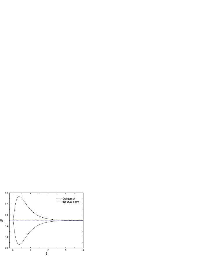
Figure 1: The evolution of Quintom-A and its dual Quintom-B as a function of time for $V=V_{0}[(\bar{\psi}\psi-b)^{2}+c]$, where $V_{0}=1.0909\times 10^{-117}$. The model parameters $b=0.05,c=10^{-3}$. The initial conditions $(\bar{\psi}\psi)_{0}=0.051$.

In succession, if $V=V_{0}[-(\bar{\psi}\psi-b)\bar{\psi}\psi+c]$, we obtain a Quintom-B model (see Ref. [43]). Taking a dual form theoretically as discuss above, we can present a numerical solution in Fig. 2. Clearly, the duality of this Spinor Quintom model shows a the evolutionary picture of Quintom-A.

Figure 2: Same as Fig.1, but for the evolution of Quintom-B and its dual Quintom-A. The solid line is the Quintom-B model, and the dash line is its dual model.

These two kinds of models describe different behaviors of the cosmological evolution: one is an expanding phase while the other lies in the contracting one. The behavior depends on the potential and initial conditions we choose. It is found that Quintom model and its dual form are symmetrical with respect to $w=-1$.

For an extended investigation, we take $V=V_{0}[(\bar{\psi}\psi-b)^{2}\bar{\psi}\psi+c]$, which can realize a picture across $w=-1$ twice. In Fig. 3, we can see that this dual model evolves from below $-1$ and crosses $-1$ twice, and later to below $-1$ again. Ultimately, it approaches to the cosmological constant boundary when $t\rightarrow+\infty$.

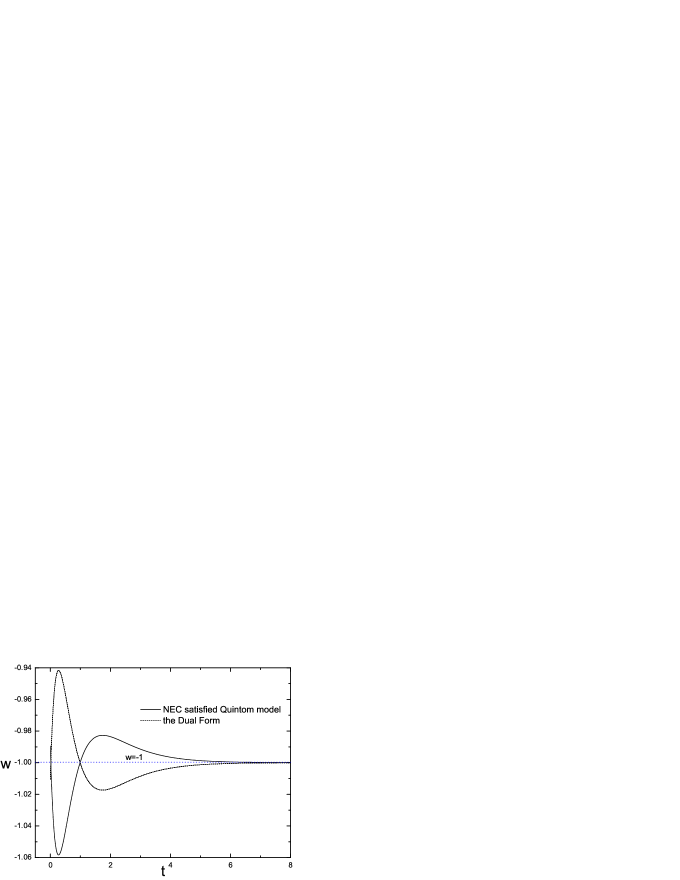
Figure 3: Same as Fig.1, but for the evolution of NEC satisfied Quintom model and its dual model. The solid line is the Quintom-B model, and the dash line is its dual model.

From the above analysis, we investigate the connections among different models and evolutionary trajectories of our universe with the help of this characteristic. It is known that under different kinds of model of evolution, the fate of the universe will be different. Our study in this section helps us understand the properties of various DE models and their connections to the evolution and the fate of the Universe. Moreover, the past and future properties can be understood by studying the above characteristics. One application to combine these properties together is Quintom-like bouncing cosmology, which has been intensively studied in Refs. [36, 37, 38]. In the meantime, we also realize three more Quitom models through the dual transformation.

III Statefinder diagnostic to Spinor Quintom models

Based on the above discussions, we have known the connections between two kinds of Spinor Quintom models. It can be seen that there are so many Spinor Quintom DE models proposed to explain the cosmic acceleration, thus how to distinguish these models become a widely attentional issue. It is no doubt that the effective EoS is an important property of DE, and different model is described by different EoS. However, the EoS, which depends on the selection of FRW background and the pre-supposition for ignorance of the contributions to the components of matter and radiation, is a model-dependent parameter[51]. In order to differentiate the different DE models fundamentally, we need a class of variables which reflect the fundamental property for field-theoretical DE models and should be independent of any assumption when the models are constructed. Considering this, we use one pair of widely used parameter—statefinder parameter—to differentiate them in this section. Also on the grounds of this consideration, Sahni proposed the geometrical–constructed from space-time metric directly– statefinder diagnostic pair $\{r,s\}$, which is defined as [50, 51],

$$r\equiv\frac{\dddot{a}}{aH^{3}},~{}~{}~{}s=\frac{r-1}{3(q-\frac{1}{2})},$$ (18)

where $q$ is the deceleration parameter,

$$q=-\frac{\ddot{a}}{aH^{2}}.$$ (19)

Accordingly, by showing different evolutionary trajectories qualitatively in the $r-s$ and $r-q$ planes, this statefinder pair can differentiate one DE model from the others. In what follows we will apply the statefinder diagnostic to three Quintom models in spinor field—Quintom-A, Quintom-B, and the Quintom model crossing $-1$ twice. We use the form of the statefinder parameter written by pressure and energy density in the following text,

$$r=1+\frac{9(\rho+p)\dot{p}}{2\rho\dot{\rho}},~{}~{}s=\frac{(\rho+p)\dot{p}}{\rho\dot{\rho}},$$ (20)

where the energy density and pressure are given by Ref. [43].

Taking components of dark matter and DE into account in a spatially flat universe, we can write down the Friedmann equation:

$$H^{2}=\frac{1}{3}(\rho_{\psi}+\rho_{m}),$$ (21)

where $\rho_{m}$ is the energy density of dark matter with EoS $p_{m}=(\gamma_{m}-1)\rho_{m}$. Ignoring the interaction between the two dark sectors, we can see that the energy density of both DE and dark matter are conserved and satisfy its continuity equation, respectively,

$$\dot{\rho_{\psi}}+3H(\rho_{\psi}+p_{\psi})=0,$$ (22)

$$\dot{\rho_{m}}+3H\rho_{m}=0.$$ (23)

As a result, using the EoS, the equation of motion and the Friedmann equation, we obtain the following expressions,

$$r = 1+\frac{9}{2}w_{\psi}(1+w_{\psi})\Omega_{\psi}+\frac{9}{2}w^{\prime}\overline{\psi}\psi\Omega_{\psi}~{},$$ (24)

$$s = 1+w_{\psi}+\frac{w^{\prime}}{w_{\psi}}\overline{\psi}\psi~{},$$ (25)

and the deceleration parameter

$$q=\frac{1}{2}+\frac{3}{2}w_{\psi}\Omega_{\psi},$$ (26)

where $\Omega_{\psi}=\frac{\rho_{\psi}}{\rho}$ is the fraction of energy density of DE, and $w^{\prime}$ is the derivative of EoS with respect to $\overline{\psi}\psi$.

Hereinafter, we study the statefinder diagnostic for the Spinor Quintom models in three different potentials. Firstly, we discuss the Quintom-A model with the form of potential $V=V_{0}[(\bar{\psi}\psi-b)^{2}+c]$, where $V_{0}$, $b$, $c$ are undefined parameters. In Fig. 4, we show the time evolution of statefinder pair $\{r,s\}$ and $\{r,q\}$. In the left figure of Fig. 4, the LCDM scenario corresponds to a fixed point $s=0,~{}r=1$. It can be found that $r$ monotonically decreases with $s$ from today to the point of LCDM along the trajectory of Spinor Quintom-A model in $r-s$ plane. The current value also can be presented.

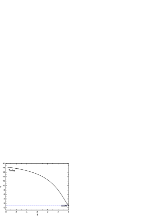
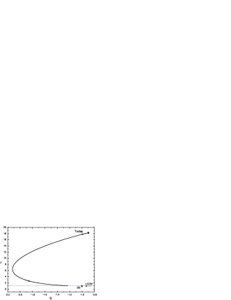
Figure 4: The $r(s)$ and $r(q)$ for the potential $V=V_{0}[(\bar{\psi}\psi-b)^{2}+c]$, where $V_{0}=1.0909\times 10^{-117}$. The model parameters $b=0.05,c=10^{-3}$. The initial conditions $(\bar{\psi}\psi)_{0}=0.051$.

Next, the trajectories of Spinor Quintom-B model with potential $V=V_{0}[-(\bar{\psi}\psi-b)\bar{\psi}\psi+c]$ are plotted. In numerical calculations, we take the same value as Quintom-A model. It can be seen that the evolutionary graphics of Quintom-B is roughly opposite to that of Quintom-A in both $\{r,s\}$ and $\{r,q\}$ planes (See Fig. 5 for a clear image). On the contrary, $r$ monotonically increases with $s$ from today to the point of $(0,1)$ corresponding to LCDM. Furthermore, this trajectory is always below that of the standard cold dark matter(SCDM).

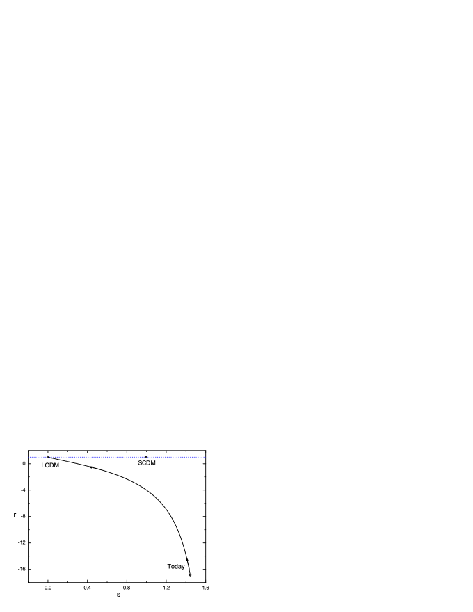
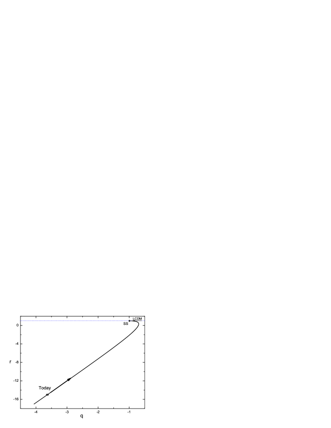
Figure 5: Same as Fig.4 but for the potential $V=V_{0}[-(\bar{\psi}\psi-b)\bar{\psi}\psi+c]$. The location of these two tracks are roughly opposite to that of Fig. 4.

Finally, we turn to the case of crossing the cosmological boundary twice. The phase portraits of $\{r,s\}$ and $\{r,q\}$ are presented in Fig. 6, respectively, where the values of parameters are also the same as those of the case of Quintom-A. In $r-s$ plane, we can see that $r$ also monotonically decreases with $s$ from today and then crosses the point of LCDM. And in final, it ends at this point. While for $r-q$ diagram, both our model and LCDM evolve to a steady state cosmology(SS) at when $q=-1,~{}r=1$, i.e. the de Sitter expansion.

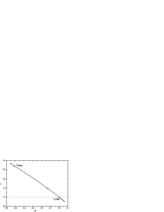
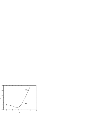
Figure 6: Same as Fig.4 but for the potential $V=V_{0}[(\bar{\psi}\psi-b)^{2}\bar{\psi}\psi+c]$.

We can see that in $r-s$ diagram both of the two former models end their evolution at the fixed point $\{r,s\}=\{1,0\}$ corresponding to the LCDM. In the case of Quintom-A, it is found that the $r-s$ phase portrait is always in the region of negative $s$ and positive $r$. On the contrary, most of the $r(s)$ trajectories of Quintom-B lies in the opposite locations. While the third case gives another evolutionary portraits. From the above numerical analysis, we find that either of these Quintom model ends their evolution at a fixed point—LCDM, in according with a De Sitter space-time realized in the second section.

In conclusion, we have investigated the dynamics of Spinor Quintom DE models by using the new geometrical diagnostic method—statefinder pair $\{r,s\}$. The Ref. [57] has applied this method to Quintom model and successfully differentiate this class of models from other DE models. But it seems not useful to discriminate Quintom models in different potentials. However, as can be seen in this section, the statefinder diagnostic is able to differentiate different Quintom models from diverse kinds of power-law potential in the spinor scenario, as well as distinguish the Spinor Quintom models from other DE models. Current data is not precise enough to distinguish these DE models by the aid of the statefinder pairs, and we expect further and more exact data to constrain the properties of DE.

IV Conclusion and Discussions

To summarize, since more and more Quintom DE models are proposed, we established the connections among these models by the aid of the cosmic duality. To connect the two totally different scenarios of universe evolution the cosmic duality in spinor scenario, we keep the energy density of the Universe and Einstein equations unchanged, but transforming the Hubble parameter. Besides, in order to make fundamental and model-independent differentiation among different DE models, we apply the new geometrical diagnostic method—statefinder pair $\{r,s\}$ to the Spinor Quintom model. We differentiate different Quintom models with different kinds of power-law potentials in the spinor scenario, and distinguish the Spinor Quintom models from other DE models, as well. As we know, the statefinder parameters $r-s$, which are the natural next step beyond the most well-known and widely used geometrical parameters Hubble parameter H(t) and the deceleration parameter q(t), relate to the third order derivatives of scalar factor. It is enough to constrain the DE models at present by the aid of this pair of parameters. However, Current data is not precise enough to distinguish these DE models, and we expect further and more exact data and the other parameters to constrain the properties of DE.

References

- [1] S. Perlmutter et al., Astrophys. J. 483, 565 (1997); Adam G. Riess et al., Astrophys. J. 116, 1009 (1998).
- [2] D. N. Spergel et al., Astrophys. J. Suppl. 148, 175 (2003).
- [3] A. G. Riess et al., Astrophys. J. 607, 665 (2004).
- [4] U. Seljak et al., Phys. Rev. D 71, 103515 (2005) [arXiv:astro-ph/0407372].
- [5] C. Wetterich, Nucl. Phys. B 302, 668 (1988).
- [6] B. Ratra and P. J. E. Peebles, Phys. Rev. D 37, 3406 (1988).
- [7] R. R. Caldwell, Phys. Lett. B 545, 23 (2002) [arXiv:astro-ph/9908168].
- [8] C. Armendariz-Picon, V. F. Mukhanov and P. J. Steinhardt, Phys. Rev. D 63, 103510 (2001) [arXiv:astro-ph/0006373].
- [9] T. Chiba, T. Okabe and M. Yamaguchi, Phys. Rev. D 62, 023511 (2000) [arXiv:astro-ph/9912463].
- [10] R. R. Caldwell, M. Kamionkowski and N. N. Weinberg, Phys. Rev. Lett. 91, 071301 (2003) [arXiv:astro-ph/0302506].
- [11] A. Y. Kamenshchik, U. Moschella and V. Pasquier, Phys. Lett. B 511, 265 (2001) [arXiv:gr-qc/0103004].
- [12] G. R. Dvali, G. Gabadadze and M. Porrati, Phys. Lett. B 485, 208 (2000) [arXiv:hep-th/0005016].
- [13] C. Deffayet, G. R. Dvali and G. Gabadadze, Phys. Rev. D 65, 044023 (2002) [arXiv:astro-ph/0105068].
- [14] W. Fischler and L. Susskind, arXiv:hep-th/9806039.
- [15] A. G. Cohen, D. B. Kaplan and A. E. Nelson, Phys. Rev. Lett. 82, 4971 (1999) [arXiv:hep-th/9803132].
- [16] S. D. H. Hsu, Phys. Lett. B 594, 13 (2004) [arXiv:hep-th/0403052].
- [17] M. Li, Phys. Lett. B 603, 1 (2004) [arXiv:hep-th/0403127].
- [18] D. N. Spergel et al. [WMAP Collaboration], Astrophys. J. Suppl. 170, 377 (2007) [arXiv:astro-ph/0603449].
- [19] E. Komatsu et al. [WMAP Collaboration], arXiv:0803.0547 [astro-ph].
- [20] A. G. Riess et al., Astrophys. J. 659, 98 (2007) [arXiv:astro-ph/0611572].
- [21] B. Feng, X. L. Wang and X. M. Zhang, Phys. Lett. B 607, 35 (2005) [arXiv:astro-ph/0404224].
- [22] G. B. Zhao, J. Q. Xia, H. Li, C. Tao, J. M. Virey, Z. H. Zhu and X. Zhang, Phys. Lett. B 648, 8 (2007) [arXiv:astro-ph/0612728].
- [23] G. B. Zhao, J. Q. Xia, B. Feng and X. Zhang, Int. J. Mod. Phys. D 16, 1229 (2007) [arXiv:astro-ph/0603621].
- [24] Y. Wang and P. Mukherjee, Astrophys. J. 650, 1 (2006) [arXiv:astro-ph/0604051].
- [25] Y. F. Cai, M. Z. Li, J. X. Lu, Y. S. Piao, T. T. Qiu and X. M. Zhang, Phys. Lett. B 651, 1 (2007) [arXiv:hep-th/0701016].
- [26] J. Q. Xia, Y. F. Cai, T. T. Qiu, G. B. Zhao and X. Zhang, Int. J. Mod. Phys. D 17, 1229 (2008) [arXiv:astro-ph/0703202].
- [27] M. Z. Li, B. Feng and X. M. Zhang, JCAP 0512, 002 (2005) [arXiv:hep-ph/0503268].
- [28] C. Armendariz-Picon, JCAP 0407, 007 (2004) [arXiv:astro-ph/0405267]; H. Wei and R. G. Cai, Phys. Rev. D 73, 083002 (2006) [arXiv:astro-ph/0603052].
- [29] T. S. Koivisto and D. F. Mota, JCAP 0808, 021 (2008) [arXiv:0805.4229 [astro-ph]].
- [30] R. G. Cai, H. S. Zhang and A. Wang, Commun. Theor. Phys. 44, 948 (2005) [arXiv:hep-th/0505186]; P. S. Apostolopoulos and N. Tetradis, Phys. Rev. D 74, 064021 (2006) [arXiv:hep-th/0604014]; K. Bamba, C. Q. Geng, S. Nojiri and S. D. Odintsov, Phys. Rev. D 79, 083014 (2009) arXiv:0810.4296 [hep-th].
- [31] I. Y. Aref’eva, A. S. Koshelev and S. Y. Vernov, Phys. Rev. D 72, 064017 (2005) [arXiv:astro-ph/0507067]; S. Y. Vernov, arXiv:astro-ph/0612487; A. S. Koshelev, JHEP 0704, 029 (2007) [arXiv:hep-th/0701103]; Y. F. Cai and W. Xue, Phys. Lett. B 680, 395 (2009) arXiv:0809.4134 [hep-th].
- [32] Z. K. Guo, Y. S. Piao, X. M. Zhang and Y. Z. Zhang, Phys. Lett. B608, 177 (2005) [arXiv:astro-ph/0410654].
- [33] X. F. Zhang, H. Li, Y. S. Piao and X. M. Zhang, Mod. Phys. Lett. A 21, 231 (2006) [arXiv:astro-ph/0501652]; Z. K. Guo, Y. S. Piao, X. Zhang and Y. Z. Zhang, Phys. Rev. D 74, 127304 (2006) [arXiv:astro-ph/0608165].
- [34] Y. F. Cai, H. Li, Y. S. Piao and X. M. Zhang, Phys. Lett. B 646, 141 (2007) [arXiv:gr-qc/0609039].
- [35] B. Feng, M. Li, Y. S. Piao and X. Zhang, Phys. Lett. B 634, 101 (2006) [arXiv:astro-ph/0407432]; H. Wei and R. G. Cai, Phys. Rev. D 72, 123507 (2005) [arXiv:astro-ph/0509328]; X. Zhang, Phys. Rev. D 74, 103505 (2006) [arXiv:astro-ph/0609699].
- [36] Y. F. Cai, T. Qiu, Y. S. Piao, M. Li and X. Zhang, JHEP 0710, 071 (2007) [arXiv:0704.1090 [gr-qc]].
- [37] quintom is found to be able to give a bouncing solution and its perturbations combine aspects of singular and nonsingular bounce models, see for example: Y. F. Cai, T. Qiu, R. Brandenberger, Y. S. Piao and X. Zhang, JCAP 0803, 013 (2008) [arXiv:0711.2187 [hep-th]]; Y. F. Cai, T. t. Qiu, R. Brandenberger and X. m. Zhang, Phys. Rev. D 80, 023511 (2009) arXiv:0810.4677 [hep-th].
- [38] Y. F. Cai, T. T. Qiu, J. Q. Xia and X. Zhang, Phys. Rev. D 79, 021303 (2009) arXiv:0808.0819 [astro-ph]; Y. F. Cai and X. Zhang, JCAP 0906, 003 (2009) arXiv:0808.2551 [astro-ph].
- [39] W. Zhao, and Y. Zhang, Phys. Rev. D 73, 123509 (2006) [arXiv:astro-ph/0604460]; H. Mohseni Sadjadi and M. Alimohammadi, Phys. Rev. D 74, 043506 (2006) [arXiv:gr-qc/0605143]; E. O. Kahya and V. K. Onemli, Phys. Rev. D 76, 043512 (2007) [arXiv:gr-qc/0612026]; Y. F. Cai and Y. S. Piao, Phys. Lett. B 657, 1 (2007) [arXiv:gr-qc/0701114]. R. Lazkoz, G. Leon and I. Quiros, Phys. Lett. B 649, 103 (2007) [arXiv:astro-ph/0701353]; H. Zhang and Z. H. Zhu, Mod. Phys. Lett. A 24, 541 (2009) arXiv:0704.3121 [astro-ph]; T. Qiu, Y. F. Cai and X. M. Zhang, Mod. Phys. Lett. A 23, 2787 (2008) arXiv:0710.0115 [gr-qc]; M. R. Setare, J. Sadeghi and A. Banijamali, Phys. Lett. B 669, 9 (2008) [arXiv:0807.0077 [hep-th]].
- [40] H. H. Xiong, T. Qiu, Y. F. Cai and X. Zhang, Mod. Phys. Lett. A 24, 1237 (2009) arXiv:0711.4469 [hep-th]; H. H. Xiong, Y. F. Cai, T. Qiu, Y. S. Piao and X. Zhang, Phys. Lett. B 666, 212 (2008) [arXiv:0805.0413 [astro-ph]]; S. Li, Y. F. Cai and Y. S. Piao, Phys. Lett. B 671, 423 (2009) arXiv:0806.2363 [hep-ph]; S. Zhang and B. Chen, Phys. Lett. B 669, 4 (2008) [arXiv:0806.4435 [hep-ph]].
- [41] E. Elizalde, S. Nojiri and S. D. Odintsov, Phys. Rev. D 70, 043539 (2004) [arXiv:hep-th/0405034].
- [42] T. Koivisto and D. F. Mota, Astrophys. J. 679, 1 (2008) [arXiv:0707.0279 [astro-ph]].
- [43] Y. F. Cai and J. Wang, Class. Quant. Grav. 25, 165014 (2008) [arXiv:0806.3890 [hep-th]].
- [44] G. Veneziano, Phys. Lett. B 265, 287 (1991).
- [45] J. E. Lidsey, D. Wands and E. J. Copeland, Phys. Rept. 337, 343 (2000) [arXiv:hep-th/9909061].
- [46] L. P. Chimento and R. Lazkoz, Phys. Rev. Lett. 91, 211301 (2003) [arXiv:gr-qc/0307111].
- [47] M. P. Dabrowski, T. Stachowiak and M. Szydlowski, Phys. Rev. D 68, 103519 (2003) [arXiv:hep-th/0307128].
- [48] L. P. Chimento and D. Pavon, Phys. Rev. D 73, 063511 (2006) [arXiv:gr-qc/0505096].
- [49] M. P. Dabrowski, C. Kiefer and B. Sandhofer, Phys. Rev. D 74, 044022 (2006) [arXiv:hep-th/0605229].
- [50] T. Chiba and T. Nakamura, Prog. Theor. Phys. 100, 1077 (1998) [arXiv:astro-ph/9808022].
- [51] V. Sahni, T. D. Saini, A. A. Starobinsky and U. Alam, JETP Lett. 77, 201 (2003) [Pisma Zh. Eksp. Teor. Fiz. 77, 249 (2003)] [arXiv:astro-ph/0201498].
- [52] W. Zimdahl and D. Pavon, Gen. Rel. Grav. 36, 1483 (2004) [arXiv:gr-qc/0311067].
- [53] U. Alam, V. Sahni, T. D. Saini and A. A. Starobinsky, Mon. Not. Roy. Astron. Soc. 344, 1057 (2003) [arXiv:astro-ph/0303009].
- [54] V. Gorini, A. Kamenshchik and U. Moschella, Phys. Rev. D 67, 063509 (2003) [arXiv:astro-ph/0209395].
- [55] X. Zhang, Phys. Lett. B 611, 1 (2005) [arXiv:astro-ph/0503075].
- [56] X. Zhang, Int. J. Mod. Phys. D 14, 1597 (2005) [arXiv:astro-ph/0504586].
- [57] P. X. Wu and H. W. Yu, Int. J. Mod. Phys. D 14, 1873 (2005) [arXiv:gr-qc/0509036].
- [58] X. Zhang, F. Q. Wu and J. Zhang, JCAP 0601, 003 (2006) [arXiv:astro-ph/0411221].
- [59] M. R. Setare, J. Zhang and X. Zhang, JCAP 0703, 007 (2007) [arXiv:gr-qc/0611084].
- [60] Z. L. Yi and T. J. Zhang, Phys. Rev. D 75, 083515 (2007) [arXiv:astro-ph/0703630].
- [61] W. Zhao, arXiv:0711.2319 [gr-qc].
- [62] G. Panotopoulos, Nucl. Phys. B 796, 66 (2008) [arXiv:0712.1177 [astro-ph]].
- [63] Z. G. Huang, X. M. Song, H. Q. Lu and W. Fang, Astrophys. Space Sci. 315, 175 (2008) [arXiv:0802.2320 [hep-th]].
- [64] Y. Shao and H. Zhong, Mod. Phys. Lett. A 23, 879 (2008).
- [65] C. J. Feng, arXiv:0809.2502 [hep-th]; C. J. Feng, arXiv:0810.2594 [hep-th].
- [66] L. P. Chimento, Phys. Rev. D 65, 063517 (2002).
- [67] J. M. Aguirregabiria, L. P. Chimento, A. S. Jakubi and R. Lazkoz, Phys. Rev. D 67, 083518 (2003) [arXiv:gr-qc/0303010].
- [68] J. M. Aguirregabiria, L. P. Chimento and R. Lazkoz, Phys. Rev. D 70, 023509 (2004) [arXiv:astro-ph/0403157].
- [69] L. P. Chimento, R. Lazkoz, Class. Quant. Grav. 23, 3195 (2006).
- [70] L. P. Chimento and W. Zimdahl, Int. J. Mod. Phys. D 17, 2229 (2008) [arXiv:gr-qc/0609104].
- [71] L. P. Chimento, F. P. Devecchi, M. Forte and G. M. Kremer, Class. Quant. Grav. 25, 085007 (2008) [arXiv:0707.4455 [gr-qc]].
- [72] C. Armendariz-Picon and P. B. Greene, Gen. Rel. Grav. 35, 1637 (2003) [arXiv:hep-th/0301129].
- [73] B. Vakili, S. Jalalzadeh and H. R. Sepangi, JCAP 0505, 006 (2005) [arXiv:gr-qc/0502076].
- [74] M. O. Ribas, F. P. Devecchi and G. M. Kremer, Phys. Rev. D 72, 123502 (2005) [arXiv:gr-qc/0511099].
- [75] S. Weinberg, Gravitation and Cosmology, Cambridge University Press (1972).
- [76] N. Birrell and P. Davies, Quantum Fields in Curved Space, Cambridge University Press (1982).
- [77] M. Green, J. Schwarz, E. Witten, Superstring Theory Vol. 2, Chapter 12, Cambridge University Press (1987).