I Introduction
In recent years photon subtracted and added quantum states have been paid
much attention because these fields exhibit an abundant of nonclassical
properties and may give access to a complete engineering of quantum states
and to fundamental quantum phenomena [1-8]. However, all these discussions
are restricted to the case at zero point temperature. In fact, most systems
are not isolated, but are immersed in a “thermal
reservoir”, excitation and de-excitation processes of a system are
influenced by its energy exchange with reservoirs. In this work we study
field properties by photon subtracting and adding at finite temperature.
The Wigner function (WF) is a powerful tool to investigate the
nonclassicality of optical fields [9,10]. Its partial negativity implies the
highly nonclassical properties of quantum states and is often used to
describe the decoherence of quantum states [7,8,11,12]. In one dimensional
case, the WF of a density matrix ρ 𝜌 \rho 𝚃𝚛 [ ρ Δ ( α ) ] , 𝚃𝚛 delimited-[] 𝜌 Δ 𝛼 \mathtt{Tr}\left[\rho\Delta(\alpha)\right], Δ ( α ) Δ 𝛼 \Delta(\alpha)
Δ ( α ) = 1 π : e − ( q − Q ) 2 − ( p − P ) 2 := 1 π : e − 2 ( α − a ) ( α ∗ − a † ) : , : Δ 𝛼 1 𝜋 assign superscript 𝑒 superscript 𝑞 𝑄 2 superscript 𝑝 𝑃 2 1 𝜋 : superscript 𝑒 2 𝛼 𝑎 superscript 𝛼 ∗ superscript 𝑎 † : absent \Delta\left(\alpha\right)=\frac{1}{\pi}\colon e^{-\left(q-Q\right)^{2}-\left(p-P\right)^{2}}\colon=\frac{1}{\pi}\colon e^{-2\left(\alpha-a\right)\left(\alpha^{\ast}-a^{\dagger}\right)}\colon, (1)
and
Δ ( α ) = 1 2 : : δ ( α − a ) δ ( α ∗ − a † ) : : , Δ 𝛼 1 2 FRACOP : : 𝛿 𝛼 𝑎 𝛿 superscript 𝛼 ∗ superscript 𝑎 † FRACOP : : \Delta\left(\alpha\right)=\frac{1}{2}\genfrac{}{}{0.0pt}{}{:}{:}\delta\left(\alpha-a\right)\delta\left(\alpha^{\ast}-a^{\dagger}\right)\genfrac{}{}{0.0pt}{}{:}{:}, (2)
where α = ( q + 𝚒 p ) / 2 , 𝛼 𝑞 𝚒 𝑝 2 \alpha=\left(q+\mathtt{i}p\right)/\sqrt{2}, a = ( Q + 𝚒 P ) / 2 𝑎 𝑄 𝚒 𝑃 2 a=\left(Q+\mathtt{i}P\right)/\sqrt{2} [ Q , P ] = 𝚒 , 𝑄 𝑃 𝚒 \left[Q,P\right]=\mathtt{i}, ℏ = 1 ; Planck-constant-over-2-pi 1 \hbar=1; a 𝑎 a a † superscript 𝑎 † a^{\dagger} [ a , a † ] = 1 ) \left[a,a^{\dagger}\right]=1) : : : absent : \colon\colon : : : : FRACOP : : FRACOP : : \genfrac{}{}{0.0pt}{}{:}{:}\genfrac{}{}{0.0pt}{}{:}{:}
S : : ( ∘ ∘ ∘ ) : : S − 1 = : : S ( ∘ ∘ ∘ ) S − 1 : : , S\genfrac{}{}{0.0pt}{}{:}{:}\left(\circ\circ\circ\right)\genfrac{}{}{0.0pt}{}{:}{:}S^{-1}=\genfrac{}{}{0.0pt}{}{:}{:}S\left(\circ\circ\circ\right)S^{-1}\genfrac{}{}{0.0pt}{}{:}{:}, (3)
as if the “fence”
: : : : FRACOP : : FRACOP : : \genfrac{}{}{0.0pt}{}{:}{:}\genfrac{}{}{0.0pt}{}{:}{:} S 𝑆 S
II Brief review of thermo state
The main point of TFD lies in converting the evaluation of ensemble average
at nonzero temperature into the equivalent expectation value with a pure
state. This worthwhile convenience is at the expense of introducing a
fictitious field (or a so-called tilde-conjugate field, denoted as operator a ~ † superscript ~ 𝑎 † \tilde{a}^{\dagger} H ~ ~ 𝐻 \tilde{H} | n ⟩ ket 𝑛 \left|n\right\rangle ℋ ℋ \mathcal{H} | n ~ ⟩ ket ~ 𝑛 \left|\tilde{n}\right\rangle H ~ ~ 𝐻 \tilde{H} a 𝑎 a ℋ ℋ \mathcal{H} a ~ ~ 𝑎 \tilde{a} H ~ ~ 𝐻 \tilde{H} T 𝑇 T | 0 ( β ) ⟩ ket 0 𝛽 \left|0(\beta)\right\rangle
⟨ A ⟩ = 𝚃𝚛 ( ρ c A ) = ⟨ 0 ( β ) | A | 0 ( β ) ⟩ = 𝚃𝚛 ( A e − β H ) / 𝚃𝚛 ( e − β H ) , delimited-⟨⟩ 𝐴 𝚃𝚛 subscript 𝜌 𝑐 𝐴 quantum-operator-product 0 𝛽 𝐴 0 𝛽 𝚃𝚛 𝐴 superscript 𝑒 𝛽 𝐻 𝚃𝚛 superscript 𝑒 𝛽 𝐻 \left\langle A\right\rangle=\mathtt{Tr}\left(\rho_{c}A\right)=\left\langle 0(\beta)\right|A\left|0(\beta)\right\rangle=\mathtt{Tr}\left(Ae^{-\beta H}\right)/\mathtt{Tr}\left(e^{-\beta H}\right), (4)
where β = 1 k T , 𝛽 1 𝑘 𝑇 \beta=\frac{1}{kT}, k 𝑘 k H 𝐻 H H 0 = ω a † a subscript 𝐻 0 𝜔 superscript 𝑎 † 𝑎 H_{0}=\omega a^{{\dagger}}a | 0 ( β ) ⟩ ket 0 𝛽 \left|0(\beta)\right\rangle
| 0 ( β ) ⟩ = sech θ exp [ a † a ~ † tanh θ ] | 0 , 0 ~ ⟩ = S ( θ ) | 0 , 0 ~ ⟩ , ket 0 𝛽 sech 𝜃 superscript 𝑎 † superscript ~ 𝑎 † 𝜃 ket 0 ~ 0
𝑆 𝜃 ket 0 ~ 0
\left|0(\beta)\right\rangle=\text{sech}\theta\exp\left[a^{\dagger}\tilde{a}^{\dagger}\tanh\theta\right]\left|0,\tilde{0}\right\rangle=S\left(\theta\right)\left|0,\tilde{0}\right\rangle, (5)
where | 0 , 0 ~ ⟩ ket 0 ~ 0
\left|0,\tilde{0}\right\rangle a 𝑎 a a ~ , ~ 𝑎 \tilde{a}, [ a ~ , a ~ † ] = 1 , ~ 𝑎 superscript ~ 𝑎 † 1 \left[\tilde{a},\tilde{a}^{\dagger}\right]=1,
S ( θ ) ≡ exp [ θ ( a † a ~ † − a a ~ ) ] , 𝑆 𝜃 𝜃 superscript 𝑎 † superscript ~ 𝑎 † 𝑎 ~ 𝑎 S\left(\theta\right)\equiv\exp\left[\theta\left(a^{\dagger}\tilde{a}^{\dagger}-a\tilde{a}\right)\right], (6)
is the thermo squeezing operator which transforms the zero-temperature
vacuum | 0 , 0 ~ ⟩ ket 0 ~ 0
\left|0,\tilde{0}\right\rangle | 0 ( β ) ⟩ , ket 0 𝛽 \left|0(\beta)\right\rangle, θ 𝜃 \theta
tanh θ = exp ( − ω 2 k T ) , 𝜃 𝜔 2 𝑘 𝑇 \tanh\theta=\exp\left(-\frac{\omega}{2kT}\right), (7)
which is determined by comparing the Bose–Einstein distribution
n c = [ exp ( ω k T ) − 1 ] − 1 subscript 𝑛 𝑐 superscript delimited-[] 𝜔 𝑘 𝑇 1 1 n_{c}=\left[\exp\left(\frac{\omega}{kT}\right)-1\right]^{-1} (8)
and
⟨ 0 ( β ) | a † a | 0 ( β ) ⟩ = sinh 2 θ . quantum-operator-product 0 𝛽 superscript 𝑎 † 𝑎 0 𝛽 superscript 2 𝜃 \left\langle 0(\beta)\right|a^{\dagger}a\left|0(\beta)\right\rangle=\sinh^{2}\theta. (9)
In particular, when operator A 𝐴 A Δ ( α ) Δ 𝛼 \Delta\left(\alpha\right)
𝚃𝚛 a ( Δ ( α ) e − β H ) / 𝚃𝚛 a ( e − β H ) subscript 𝚃𝚛 𝑎 Δ 𝛼 superscript 𝑒 𝛽 𝐻 subscript 𝚃𝚛 𝑎 superscript 𝑒 𝛽 𝐻 \displaystyle\mathtt{Tr}_{a}\left(\Delta\left(\alpha\right)e^{-\beta H}\right)/\mathtt{Tr}_{a}\left(e^{-\beta H}\right) = \displaystyle= ⟨ 0 ( β ) | Δ ( α ) | 0 ( β ) ⟩ quantum-operator-product 0 𝛽 Δ 𝛼 0 𝛽 \displaystyle\left\langle 0(\beta)\right|\Delta\left(\alpha\right)\left|0(\beta)\right\rangle (10)
= \displaystyle= 𝚃𝚛 a , a ~ [ Δ ( α ) | 0 ( β ) ⟩ ⟨ 0 ( β ) | ] , subscript 𝚃𝚛 𝑎 ~ 𝑎
delimited-[] Δ 𝛼 ket 0 𝛽 bra 0 𝛽 \displaystyle\mathtt{Tr}_{a,\tilde{a}}\left[\Delta\left(\alpha\right)\left|0(\beta)\right\rangle\left\langle 0(\beta)\right|\right],
which is just the WF of thermo vacuum state. From Eq.(10 | 0 ( β ) ⟩ ket 0 𝛽 \left|0(\beta)\right\rangle ρ c → | 0 ( β ) ⟩ ⟨ 0 ( β ) | → subscript 𝜌 𝑐 ket 0 𝛽 bra 0 𝛽 \rho_{c}\rightarrow\left|0(\beta)\right\rangle\left\langle 0(\beta)\right|
III Normally ordered form of S † ( θ ) Δ ( α ) S ( θ ) superscript 𝑆 † 𝜃 Δ 𝛼 𝑆 𝜃 S^{\dagger}\left(\theta\right)\Delta\left(\alpha\right)S\left(\theta\right)
In order to deriving conveniently the WFs of density operators at finite
temperature, let’s first calculate the normally ordered form of S † ( θ ) Δ ( α ) S ( θ ) . superscript 𝑆 † 𝜃 Δ 𝛼 𝑆 𝜃 S^{\dagger}\left(\theta\right)\Delta\left(\alpha\right)S\left(\theta\right).
H ^ ( a , a † ) = 2 ∫ 𝚍 2 α h ( α , α ∗ ) Δ ( α ) , ^ 𝐻 𝑎 superscript 𝑎 † 2 superscript 𝚍 2 𝛼 ℎ 𝛼 superscript 𝛼 ∗ Δ 𝛼 \hat{H}\left(a,a^{{\dagger}}\right)=2\int\mathtt{d}^{2}\alpha h\left(\alpha,\alpha^{\ast}\right)\Delta\left(\alpha\right), (11)
where h ( α , α ∗ ) ℎ 𝛼 superscript 𝛼 ∗ h\left(\alpha,\alpha^{\ast}\right) H ^ ( a , a † ) . ^ 𝐻 𝑎 superscript 𝑎 † \hat{H}\left(a,a^{{\dagger}}\right). 11 2
H ^ ( a , a † ) ^ 𝐻 𝑎 superscript 𝑎 † \displaystyle\hat{H}\left(a,a^{{\dagger}}\right) = \displaystyle= ∫ 𝚍 2 α h ( α , α ∗ ) : : δ ( α − a ) δ ( α ∗ − a † ) : : superscript 𝚍 2 𝛼 ℎ 𝛼 superscript 𝛼 ∗ FRACOP : : 𝛿 𝛼 𝑎 𝛿 superscript 𝛼 ∗ superscript 𝑎 † FRACOP : : \displaystyle\int\mathtt{d}^{2}\alpha h\left(\alpha,\alpha^{\ast}\right)\genfrac{}{}{0.0pt}{}{:}{:}\delta\left(\alpha-a\right)\delta\left(\alpha^{\ast}-a^{\dagger}\right)\genfrac{}{}{0.0pt}{}{:}{:} (12)
= \displaystyle= : : h ( a , a † ) : : , FRACOP : : ℎ 𝑎 superscript 𝑎 † FRACOP : : \displaystyle\genfrac{}{}{0.0pt}{}{:}{:}h\left(a,a^{\dagger}\right)\genfrac{}{}{0.0pt}{}{:}{:},
which means that Weyl ordered of operator
: : h ( a , a † ) : : FRACOP : : ℎ 𝑎 superscript 𝑎 † FRACOP : : \genfrac{}{}{0.0pt}{}{:}{:}h\left(a,a^{\dagger}\right)\genfrac{}{}{0.0pt}{}{:}{:} h ( α , α ∗ ) ℎ 𝛼 superscript 𝛼 ∗ h\left(\alpha,\alpha^{\ast}\right) α , α ∗ 𝛼 superscript 𝛼 ∗
\alpha,\alpha^{\ast} h ( α , α ∗ ) ℎ 𝛼 superscript 𝛼 ∗ h\left(\alpha,\alpha^{\ast}\right) a 𝑎 a a † superscript 𝑎 † a^{\dagger} h ℎ h
According to the Weyl ordering invariance under similar transformations [13]
and the following transform relation
S † ( θ ) a S ( θ ) superscript 𝑆 † 𝜃 𝑎 𝑆 𝜃 \displaystyle S^{\dagger}\left(\theta\right)aS\left(\theta\right) = \displaystyle= a cosh θ + a ~ † sinh θ , 𝑎 𝜃 superscript ~ 𝑎 † 𝜃 \displaystyle a\cosh\theta+\tilde{a}^{\dagger}\sinh\theta,
S † ( θ ) a ~ S ( θ ) superscript 𝑆 † 𝜃 ~ 𝑎 𝑆 𝜃 \displaystyle S^{\dagger}\left(\theta\right)\tilde{a}S\left(\theta\right) = \displaystyle= a ~ cosh θ + a † sinh θ , ~ 𝑎 𝜃 superscript 𝑎 † 𝜃 \displaystyle\tilde{a}\cosh\theta+a^{\dagger}\sinh\theta, (13)
it is easily seen
S † ( θ ) Δ ( α ) S ( θ ) superscript 𝑆 † 𝜃 Δ 𝛼 𝑆 𝜃 \displaystyle S^{\dagger}\left(\theta\right)\Delta\left(\alpha\right)S\left(\theta\right) = \displaystyle= 1 2 : : δ ( α − a cosh θ − a ~ † sinh θ ) 1 2 FRACOP : : 𝛿 𝛼 𝑎 𝜃 superscript ~ 𝑎 † 𝜃 \displaystyle\frac{1}{2}\genfrac{}{}{0.0pt}{}{:}{:}\delta\left(\alpha-a\cosh\theta-\tilde{a}^{\dagger}\sinh\theta\right) (14)
× δ ( α ∗ − a † cosh θ − a ~ sinh θ ) : : , absent 𝛿 superscript 𝛼 ∗ superscript 𝑎 † 𝜃 ~ 𝑎 𝜃 FRACOP : : \displaystyle\times\delta\left(\alpha^{\ast}-a^{{\dagger}}\cosh\theta-\tilde{a}\sinh\theta\right)\genfrac{}{}{0.0pt}{}{:}{:},
which is just the Weyl ordering of S † ( θ ) Δ ( α ) S ( θ ) superscript 𝑆 † 𝜃 Δ 𝛼 𝑆 𝜃 S^{\dagger}\left(\theta\right)\Delta\left(\alpha\right)S\left(\theta\right) h ( β , β ∗ ; β ~ , β ~ ∗ ) ℎ 𝛽 superscript 𝛽 ∗ ~ 𝛽 superscript ~ 𝛽 ∗ h\left(\beta,\beta^{\ast};\tilde{\beta},\tilde{\beta}^{\ast}\right) S † ( θ ) Δ ( α ) S ( θ ) superscript 𝑆 † 𝜃 Δ 𝛼 𝑆 𝜃 S^{\dagger}\left(\theta\right)\Delta\left(\alpha\right)S\left(\theta\right) a , a † ) a,a^{{\dagger}}) a ~ , a ~ † ) \tilde{a},\tilde{a}^{{\dagger}}) β , β ∗ 𝛽 superscript 𝛽 ∗
\beta,\beta^{\ast} β ~ , β ~ ∗ ) \tilde{\beta},\tilde{\beta}^{\ast})
h ( β , β ∗ ; β ~ , β ~ ∗ ) ℎ 𝛽 superscript 𝛽 ∗ ~ 𝛽 superscript ~ 𝛽 ∗ \displaystyle h\left(\beta,\beta^{\ast};\tilde{\beta},\tilde{\beta}^{\ast}\right) = \displaystyle= 1 2 δ ( α − β cosh θ − β ~ ∗ sinh θ ) 1 2 𝛿 𝛼 𝛽 𝜃 superscript ~ 𝛽 ∗ 𝜃 \displaystyle\frac{1}{2}\delta\left(\alpha-\beta\cosh\theta-\tilde{\beta}^{\ast}\sinh\theta\right) (15)
× δ ( α ∗ − β ∗ cosh θ − β ~ sinh θ ) . absent 𝛿 superscript 𝛼 ∗ superscript 𝛽 ∗ 𝜃 ~ 𝛽 𝜃 \displaystyle\times\delta\left(\alpha^{\ast}-\beta^{\ast}\cosh\theta-\tilde{\beta}\sinh\theta\right).
It then follows from Eqs.(11 15
S † ( θ ) Δ ( α ) S ( θ ) = 4 ∫ 𝚍 2 β 𝚍 2 β ~ Δ ( β , β ∗ ; β ~ , β ~ ∗ ) h ( β , β ∗ ; β ~ , β ~ ∗ ) , superscript 𝑆 † 𝜃 Δ 𝛼 𝑆 𝜃 4 superscript 𝚍 2 𝛽 superscript 𝚍 2 ~ 𝛽 Δ 𝛽 superscript 𝛽 ∗ ~ 𝛽 superscript ~ 𝛽 ∗ ℎ 𝛽 superscript 𝛽 ∗ ~ 𝛽 superscript ~ 𝛽 ∗ S^{\dagger}\left(\theta\right)\Delta\left(\alpha\right)S\left(\theta\right)=4\int\mathtt{d}^{2}\beta\mathtt{d}^{2}\tilde{\beta}\Delta\left(\beta,\beta^{\ast};\tilde{\beta},\tilde{\beta}^{\ast}\right)h\left(\beta,\beta^{\ast};\tilde{\beta},\tilde{\beta}^{\ast}\right), (16)
where Δ ( β , β ∗ ; β ~ , β ~ ∗ ) Δ 𝛽 superscript 𝛽 ∗ ~ 𝛽 superscript ~ 𝛽 ∗ \Delta\left(\beta,\beta^{\ast};\tilde{\beta},\tilde{\beta}^{\ast}\right)
Δ ( β , β ∗ ; β ~ , β ~ ∗ ) = 1 π 2 : exp [ − 2 ( a † − β ∗ ) ( a − β ) − 2 ( a ~ † − β ~ ∗ ) ( a ~ − β ~ ) ] : . : Δ 𝛽 superscript 𝛽 ∗ ~ 𝛽 superscript ~ 𝛽 ∗ 1 superscript 𝜋 2 2 superscript 𝑎 † superscript 𝛽 ∗ 𝑎 𝛽 2 superscript ~ 𝑎 † superscript ~ 𝛽 ∗ ~ 𝑎 ~ 𝛽 : absent \Delta\left(\beta,\beta^{\ast};\tilde{\beta},\tilde{\beta}^{\ast}\right)=\frac{1}{\pi^{2}}\colon\exp\left[-2\left(a^{{\dagger}}-\beta^{\ast}\right)\left(a-\beta\right)-2\left(\tilde{a}^{{\dagger}}-\tilde{\beta}^{\ast}\right)\left(\tilde{a}-\tilde{\beta}\right)\right]\colon. (17)
On substituting Eq.(17 16
∫ 𝚍 2 z π e ζ | z | 2 + ξ z + η z ∗ = − 1 ζ e − ξ η ζ , Re ( ζ ) < 0 , formulae-sequence superscript 𝚍 2 𝑧 𝜋 superscript 𝑒 𝜁 superscript 𝑧 2 𝜉 𝑧 𝜂 superscript 𝑧 ∗ 1 𝜁 superscript 𝑒 𝜉 𝜂 𝜁 Re 𝜁 0 \int\frac{\mathtt{d}^{2}z}{\pi}e^{\zeta\left|z\right|^{2}+\xi z+\eta z^{\ast}}=-\frac{1}{\zeta}e^{-\frac{\xi\eta}{\zeta}},\text{ Re}\left(\zeta\right)<0, (18)
we can derive the normally ordered form of (16
S † ( θ ) Δ ( α ) S ( θ ) superscript 𝑆 † 𝜃 Δ 𝛼 𝑆 𝜃 \displaystyle S^{\dagger}\left(\theta\right)\Delta\left(\alpha\right)S\left(\theta\right) = \displaystyle= 2 ∫ 𝚍 2 β 𝚍 2 β ~ π 2 δ ( α − β cosh θ − β ~ ∗ sinh θ ) 2 superscript 𝚍 2 𝛽 superscript 𝚍 2 ~ 𝛽 superscript 𝜋 2 𝛿 𝛼 𝛽 𝜃 superscript ~ 𝛽 ∗ 𝜃 \displaystyle 2\int\frac{\mathtt{d}^{2}\beta\mathtt{d}^{2}\tilde{\beta}}{\pi^{2}}\delta\left(\alpha-\beta\cosh\theta-\tilde{\beta}^{\ast}\sinh\theta\right) (19)
× δ ( α ∗ − β ∗ cosh θ − β ~ sinh θ ) absent 𝛿 superscript 𝛼 ∗ superscript 𝛽 ∗ 𝜃 ~ 𝛽 𝜃 \displaystyle\times\delta\left(\alpha^{\ast}-\beta^{\ast}\cosh\theta-\tilde{\beta}\sinh\theta\right)
× : exp [ − 2 ( a † − β ∗ ) ( a − β ) − 2 ( a ~ † − β ~ ∗ ) ( a ~ − β ~ ) ] : \displaystyle\times\colon\exp\left[-2\left(a^{{\dagger}}-\beta^{\ast}\right)\left(a-\beta\right)-2\left(\tilde{a}^{{\dagger}}-\tilde{\beta}^{\ast}\right)\left(\tilde{a}-\tilde{\beta}\right)\right]\colon
= \displaystyle= sech 2 θ π e − 2 | α | 2 sech 2 θ : exp { − ( a a ~ + a † a ~ † ) tanh 2 θ \displaystyle\frac{\text{sech}2\theta}{\pi}e^{-2\left|\alpha\right|^{2}\text{sech}2\theta}\colon\exp\left\{-\left(a\tilde{a}+a^{{\dagger}}\tilde{a}^{{\dagger}}\right)\tanh 2\theta\right.
+ 2 sech 2 θ [ sinh θ ( α ∗ a ~ † + α a ~ ) + cosh θ ( α ∗ a + α a † ) \displaystyle+2\text{sech}2\theta\left[\sinh\theta\left(\allowbreak\alpha^{\ast}\tilde{a}^{{\dagger}}+\allowbreak\alpha\tilde{a}\right)+\cosh\theta\left(\alpha^{\ast}a+\alpha a^{\dagger}\right)\right.
− ( a ~ † a ~ sinh 2 θ + a † a cosh 2 θ ) ] } : , \displaystyle-\left(\tilde{a}^{{\dagger}}\tilde{a}\sinh^{2}\theta+a^{{\dagger}}a\cosh^{2}\theta\right)]\}\colon,
which is just the normally ordered form of (16 19 | 0 ( β ) ⟩ ket 0 𝛽 \left|0(\beta)\right\rangle
⟨ 0 ( β ) | Δ ( α ) | 0 ( β ) ⟩ quantum-operator-product 0 𝛽 Δ 𝛼 0 𝛽 \displaystyle\left\langle 0(\beta)\right|\Delta\left(\alpha\right)\left|0(\beta)\right\rangle = \displaystyle= ⟨ 0 , 0 ~ | S † ( θ ) Δ ( α ) S ( θ ) | 0 , 0 ~ ⟩ = sech 2 θ π e − 2 | α | 2 sech 2 θ quantum-operator-product 0 ~ 0
superscript 𝑆 † 𝜃 Δ 𝛼 𝑆 𝜃 0 ~ 0
sech 2 𝜃 𝜋 superscript 𝑒 2 superscript 𝛼 2 sech 2 𝜃 \displaystyle\left\langle 0,\tilde{0}\right|S^{\dagger}\left(\theta\right)\Delta\left(\alpha\right)S\left(\theta\right)\left|0,\tilde{0}\right\rangle=\frac{\text{sech}2\theta}{\pi}e^{-2\left|\alpha\right|^{2}\text{sech}2\theta} (20)
= \displaystyle= 1 − e − β ω π ( 1 + e − β ω ) e − 2 | α | 2 1 − e − β ω 1 + e − β ω . 1 superscript 𝑒 𝛽 𝜔 𝜋 1 superscript 𝑒 𝛽 𝜔 superscript 𝑒 2 superscript 𝛼 2 1 superscript 𝑒 𝛽 𝜔 1 superscript 𝑒 𝛽 𝜔 \displaystyle\frac{1-e^{-\beta\omega}}{\pi(1+e^{-\beta\omega})}e^{-2\left|\alpha\right|^{2}\frac{1-e^{-\beta\omega}}{1+e^{-\beta\omega}}}.
IV Wigner function of photon-subtracted thermo vacuum state
At finite temperature, the photon-subtracted thermo vacuum state can be
expressed as [20]
ρ 1 = C 1 a n | 0 ( β ) ⟩ ⟨ 0 ( β ) | a † n , subscript 𝜌 1 subscript 𝐶 1 superscript 𝑎 𝑛 ket 0 𝛽 bra 0 𝛽 superscript 𝑎 † absent 𝑛 \rho_{1}=C_{1}a^{n}\left|0(\beta)\right\rangle\left\langle 0(\beta)\right|a^{{\dagger}n}, (21)
where C 1 subscript 𝐶 1 C_{1}
C 1 − 1 = 𝚃𝚛 [ a n S ( θ ) | 0 , 0 ~ ⟩ ⟨ 0 , 0 ~ | S † ( θ ) a † n ] , C_{1}^{-1}=\mathtt{Tr}\left[a^{n}S\left(\theta\right)\left|0,\tilde{0}\right\rangle\left\langle 0,\tilde{0}\right|S^{{\dagger}}\left(\theta\right)a^{{\dagger}n}\right], (22)
which can be calculated as follows. Using Eq.(5
∑ l = 0 ∞ ( n + l ) ! n ! l ! x l = ( 1 − x ) − n − 1 , superscript subscript 𝑙 0 𝑛 𝑙 𝑛 𝑙 superscript 𝑥 𝑙 superscript 1 𝑥 𝑛 1 \sum_{l=0}^{\infty}\frac{\left(n+l\right)!}{n!l!}x^{l}=\left(1-x\right)^{-n-1}, (23)
we have
C 1 − 1 superscript subscript 𝐶 1 1 \displaystyle C_{1}^{-1} = \displaystyle= ⟨ 0 , 0 ~ | S † ( θ ) a † n a n S ( θ ) | 0 , 0 ~ ⟩ quantum-operator-product 0 ~ 0
superscript 𝑆 † 𝜃 superscript 𝑎 † absent 𝑛 superscript 𝑎 𝑛 𝑆 𝜃 0 ~ 0
\displaystyle\left\langle 0,\tilde{0}\right|S^{{\dagger}}\left(\theta\right)a^{{\dagger}n}a^{n}S\left(\theta\right)\left|0,\tilde{0}\right\rangle (24)
= \displaystyle= sech 2 θ ⟨ 0 , 0 ~ | e a a ~ tanh θ a † n a n e a † a ~ † tanh θ | 0 , 0 ~ ⟩ superscript sech 2 𝜃 quantum-operator-product 0 ~ 0
superscript 𝑒 𝑎 ~ 𝑎 𝜃 superscript 𝑎 † absent 𝑛 superscript 𝑎 𝑛 superscript 𝑒 superscript 𝑎 † superscript ~ 𝑎 † 𝜃 0 ~ 0
\displaystyle\text{sech}^{2}\theta\left\langle 0,\tilde{0}\right|e^{a\tilde{a}\tanh\theta}a^{{\dagger}n}a^{n}e^{a^{\dagger}\tilde{a}^{\dagger}\tanh\theta}\left|0,\tilde{0}\right\rangle
= \displaystyle= sech 2 θ ∑ k , l = 0 ∞ tanh l + k θ ⟨ k , k ~ | a † n a n | l , l ~ ⟩ superscript sech 2 𝜃 superscript subscript 𝑘 𝑙
0 superscript 𝑙 𝑘 𝜃 quantum-operator-product 𝑘 ~ 𝑘
superscript 𝑎 † absent 𝑛 superscript 𝑎 𝑛 𝑙 ~ 𝑙
\displaystyle\text{sech}^{2}\theta\sum_{k,l=0}^{\infty}\tanh^{l+k}\theta\left\langle k,\tilde{k}\right|a^{{\dagger}n}a^{n}\left|l,\tilde{l}\right\rangle
= \displaystyle= sech 2 θ ∑ l = n ∞ l ! ( l − n ) ! tanh 2 l θ = n ! sinh 2 n θ . superscript sech 2 𝜃 superscript subscript 𝑙 𝑛 𝑙 𝑙 𝑛 superscript 2 𝑙 𝜃 𝑛 superscript 2 𝑛 𝜃 \displaystyle\text{sech}^{2}\theta\sum_{l=n}^{\infty}\frac{l!}{\left(l-n\right)!}\tanh^{2l}\theta=n!\sinh^{2n}\theta.
By using Eqs. (21 19 ρ 1 subscript 𝜌 1 \rho_{1}
W 1 ( α ) subscript 𝑊 1 𝛼 \displaystyle W_{1}\left(\alpha\right) = \displaystyle= C 1 ⟨ 0 , 0 ~ | S † ( θ ) a † n Δ ( α ) a n S ( θ ) | 0 , 0 ~ ⟩ subscript 𝐶 1 quantum-operator-product 0 ~ 0
superscript 𝑆 † 𝜃 superscript 𝑎 † absent 𝑛 Δ 𝛼 superscript 𝑎 𝑛 𝑆 𝜃 0 ~ 0
\displaystyle C_{1}\left\langle 0,\tilde{0}\right|S^{{\dagger}}\left(\theta\right)a^{{\dagger}n}\Delta\left(\alpha\right)a^{n}S\left(\theta\right)\left|0,\tilde{0}\right\rangle (25)
= \displaystyle= ⟨ 0 , 0 ~ | [ S † ( θ ) a † n S ( θ ) ] S † ( θ ) Δ ( α ) S ( θ ) [ S † ( θ ) a n S ( θ ) ] | 0 , 0 ~ ⟩ . quantum-operator-product 0 ~ 0
delimited-[] superscript 𝑆 † 𝜃 superscript 𝑎 † absent 𝑛 𝑆 𝜃 superscript 𝑆 † 𝜃 Δ 𝛼 𝑆 𝜃 delimited-[] superscript 𝑆 † 𝜃 superscript 𝑎 𝑛 𝑆 𝜃 0 ~ 0
\displaystyle\left\langle 0,\tilde{0}\right|\left[S^{{\dagger}}\left(\theta\right)a^{{\dagger}n}S\left(\theta\right)\right]S^{{\dagger}}\left(\theta\right)\Delta\left(\alpha\right)S\left(\theta\right)\left[S^{{\dagger}}\left(\theta\right)a^{n}S\left(\theta\right)\right]\left|0,\tilde{0}\right\rangle.
Noticing Eq.(13
[ S † ( θ ) a n S ( θ ) ] | 0 , 0 ~ ⟩ delimited-[] superscript 𝑆 † 𝜃 superscript 𝑎 𝑛 𝑆 𝜃 ket 0 ~ 0
\displaystyle\left[S^{{\dagger}}\left(\theta\right)a^{n}S\left(\theta\right)\right]\left|0,\tilde{0}\right\rangle = \displaystyle= ( a cosh θ + a ~ † sinh θ ) n | 0 , 0 ~ ⟩ superscript 𝑎 𝜃 superscript ~ 𝑎 † 𝜃 𝑛 ket 0 ~ 0
\displaystyle\left(a\cosh\theta+\tilde{a}^{\dagger}\sinh\theta\right)^{n}\left|0,\tilde{0}\right\rangle (26)
= \displaystyle= n ! sinh n θ | 0 , n ~ ⟩ , 𝑛 superscript 𝑛 𝜃 ket 0 ~ 𝑛
\displaystyle\sqrt{n!}\sinh^{n}\theta\left|0,\tilde{n}\right\rangle,
then substituting (26 25 19
W 1 ( α ) subscript 𝑊 1 𝛼 \displaystyle W_{1}\left(\alpha\right) = \displaystyle= e − 2 | α | 2 sech 2 θ π cosh 2 θ ⟨ n ~ | e 2 sinh θ cosh 2 θ α ∗ a ~ † ( sech 2 θ ) a ~ † a ~ e 2 sinh θ cosh 2 θ a ~ α | n ~ ⟩ superscript 𝑒 2 superscript 𝛼 2 sech 2 𝜃 𝜋 2 𝜃 quantum-operator-product ~ 𝑛 superscript 𝑒 2 𝜃 2 𝜃 superscript 𝛼 ∗ superscript ~ 𝑎 † superscript sech 2 𝜃 superscript ~ 𝑎 † ~ 𝑎 superscript 𝑒 2 𝜃 2 𝜃 ~ 𝑎 𝛼 ~ 𝑛 \displaystyle\frac{e^{-2\left|\alpha\right|^{2}\text{sech}2\theta}}{\pi\cosh 2\theta}\left\langle\tilde{n}\right|e^{\frac{2\sinh\theta}{\cosh 2\theta}\alpha^{\ast}\tilde{a}^{{\dagger}}}\left(\text{sech}2\theta\right)^{\tilde{a}^{{\dagger}}\tilde{a}}e^{\frac{2\sinh\theta}{\cosh 2\theta}\tilde{a}\alpha}\left|\tilde{n}\right\rangle (27)
= \displaystyle= e − 2 | α | 2 sech 2 θ π cosh 2 θ ∑ k , l = 0 n α ∗ k α l k ! l ! ( 2 sinh θ cosh 2 θ ) k + l ⟨ n ~ | a ~ † k ( sech 2 θ ) a ~ † a ~ a ~ l | n ~ ⟩ superscript 𝑒 2 superscript 𝛼 2 sech 2 𝜃 𝜋 2 𝜃 superscript subscript 𝑘 𝑙
0 𝑛 superscript 𝛼 ∗ absent 𝑘 superscript 𝛼 𝑙 𝑘 𝑙 superscript 2 𝜃 2 𝜃 𝑘 𝑙 quantum-operator-product ~ 𝑛 superscript ~ 𝑎 † absent 𝑘 superscript sech 2 𝜃 superscript ~ 𝑎 † ~ 𝑎 superscript ~ 𝑎 𝑙 ~ 𝑛 \displaystyle\frac{e^{-2\left|\alpha\right|^{2}\text{sech}2\theta}}{\pi\cosh 2\theta}\sum_{k,l=0}^{n}\frac{\alpha^{\ast k}\alpha^{l}}{k!l!}\left(\frac{2\sinh\theta}{\cosh 2\theta}\right)^{k+l}\left\langle\tilde{n}\right|\tilde{a}^{{\dagger}k}\left(\text{sech}2\theta\right)^{\tilde{a}^{{\dagger}}\tilde{a}}\tilde{a}^{l}\left|\tilde{n}\right\rangle
= \displaystyle= e − 2 | α | 2 sech 2 θ π cosh n + 1 2 θ ∑ l = 0 n n ! l ! l ! ( n − l ) ! ( 4 sinh 2 θ cosh 2 θ | α | 2 ) l , superscript 𝑒 2 superscript 𝛼 2 sech 2 𝜃 𝜋 superscript 𝑛 1 2 𝜃 superscript subscript 𝑙 0 𝑛 𝑛 𝑙 𝑙 𝑛 𝑙 superscript 4 superscript 2 𝜃 2 𝜃 superscript 𝛼 2 𝑙 \displaystyle\frac{e^{-2\left|\alpha\right|^{2}\text{sech}2\theta}}{\pi\cosh^{n+1}2\theta}\sum_{l=0}^{n}\frac{n!}{l!l!\left(n-l\right)!}\left(\frac{4\sinh^{2}\theta}{\cosh 2\theta}\left|\alpha\right|^{2}\right)^{l},
where we have used the identity operator [21]
exp [ λ a ~ † a ~ ] = : exp [ ( e λ − 1 ) a ~ † a ~ ] : . \exp\left[\lambda\tilde{a}^{{\dagger}}\tilde{a}\right]=\colon\exp\left[\left(e^{\lambda}-1\right)\tilde{a}^{{\dagger}}\tilde{a}\right]\colon. (28)
Recalling that the definition of Laguerre polynomials [22],
L n ( x ) = ∑ l = 0 n n ! ( l ! ) 2 ( n − l ) ! ( − x ) l , subscript 𝐿 𝑛 𝑥 superscript subscript 𝑙 0 𝑛 𝑛 superscript 𝑙 2 𝑛 𝑙 superscript 𝑥 𝑙 L_{n}(x)=\sum_{l=0}^{n}\frac{n!}{\left(l!\right)^{2}\left(n-l\right)!}(-x)^{l}, (29)
Eq. (27
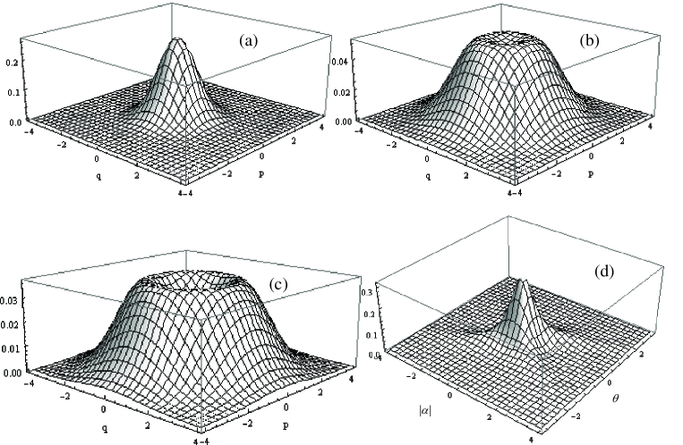
W 1 ( α ) = e − 2 | α | 2 sech 2 θ π cosh n + 1 2 θ L n ( − 4 sinh 2 θ cosh 2 θ | α | 2 ) , subscript 𝑊 1 𝛼 superscript 𝑒 2 superscript 𝛼 2 sech 2 𝜃 𝜋 superscript 𝑛 1 2 𝜃 subscript 𝐿 𝑛 4 superscript 2 𝜃 2 𝜃 superscript 𝛼 2 W_{1}\left(\alpha\right)=\frac{e^{-2\left|\alpha\right|^{2}\text{sech}2\theta}}{\pi\cosh^{n+1}2\theta}L_{n}\left(-\frac{4\sinh^{2}\theta}{\cosh 2\theta}\left|\alpha\right|^{2}\right), (30)
which is just the WF of photon-subtracted thermo vacuum state, a
Gaussian-Laguerre type function of temperature, since tanh θ = exp ( − ω 2 k T ) 𝜃 𝜔 2 𝑘 𝑇 \tanh\theta=\exp\left(-\frac{\omega}{2kT}\right) cosh 2 θ > 0 2 𝜃 0 \cosh 2\theta>0 L n ( − 4 sinh 2 θ cosh 2 θ | α | 2 ) ⩾ 0 subscript 𝐿 𝑛 4 superscript 2 𝜃 2 𝜃 superscript 𝛼 2 0 L_{n}(-\frac{4\sinh^{2}\theta}{\cosh 2\theta}\left|\alpha\right|^{2})\geqslant 0 W 1 ( α ) subscript 𝑊 1 𝛼 W_{1}\left(\alpha\right) ( | α | , θ ) 𝛼 𝜃 \left(\left|\alpha\right|,\theta\right) θ 𝜃 \theta 30 30 more concise and convenient for further
discussion.
Figure 1: Wigner function distributions of photon-subtracted thermo state in (q , p 𝑞 𝑝
q,p n = 1 , θ = 0.2 formulae-sequence 𝑛 1 𝜃 0.2 n=1,\theta=0.2 n = 1 , θ = 0.8 formulae-sequence 𝑛 1 𝜃 0.8 n=1,\theta=0.8 n = 2 , θ = 0.8 formulae-sequence 𝑛 2 𝜃 0.8 n=2,\theta=0.8 ( | α | , θ ) 𝛼 𝜃 \left(\left|\alpha\right|,\theta\right) n = 1 𝑛 1 n=1
V Wigner function of photon-added thermo vacuum state
At finite temperature, the photon-added thermo vacuum state is expressed as
[23]
ρ 2 = C 2 a † n | 0 ( β ) ⟩ ⟨ 0 ( β ) | a n . subscript 𝜌 2 subscript 𝐶 2 superscript 𝑎 † absent 𝑛 ket 0 𝛽 bra 0 𝛽 superscript 𝑎 𝑛 \rho_{2}=C_{2}a^{{\dagger}n}\left|0(\beta)\right\rangle\left\langle 0(\beta)\right|a^{n}. (31)
By the same procedures as deriving Eqs. (22 26
C 2 − 1 = n ! cosh 2 n θ , superscript subscript 𝐶 2 1 𝑛 superscript 2 𝑛 𝜃 C_{2}^{-1}=n!\cosh^{2n}\theta, (32)
and
S † ( θ ) a † n S ( θ ) | 0 , 0 ~ ⟩ = n ! cosh n θ | n , 0 ~ ⟩ . superscript 𝑆 † 𝜃 superscript 𝑎 † absent 𝑛 𝑆 𝜃 ket 0 ~ 0
𝑛 superscript 𝑛 𝜃 ket 𝑛 ~ 0
S^{{\dagger}}\left(\theta\right)a^{{\dagger}n}S\left(\theta\right)\left|0,\tilde{0}\right\rangle=\sqrt{n!}\cosh^{n}\theta\left|n,\tilde{0}\right\rangle. (33)
Uisng Eq.(32 33 W 2 ( α ) subscript 𝑊 2 𝛼 W_{2}\left(\alpha\right) ρ 2 subscript 𝜌 2 \rho_{2}\
W 2 ( α ) subscript 𝑊 2 𝛼 \displaystyle W_{2}\left(\alpha\right) = \displaystyle= C 2 ⟨ 0 , 0 ~ | S † ( θ ) a n S ( θ ) [ S † ( θ ) Δ ( α ) S ( θ ) ] S † ( θ ) a † n S ( θ ) | 0 , 0 ~ ⟩ subscript 𝐶 2 quantum-operator-product 0 ~ 0
superscript 𝑆 † 𝜃 superscript 𝑎 𝑛 𝑆 𝜃 delimited-[] superscript 𝑆 † 𝜃 Δ 𝛼 𝑆 𝜃 superscript 𝑆 † 𝜃 superscript 𝑎 † absent 𝑛 𝑆 𝜃 0 ~ 0
\displaystyle C_{2}\left\langle 0,\tilde{0}\right|S^{{\dagger}}\left(\theta\right)a^{n}S\left(\theta\right)\left[S^{{\dagger}}\left(\theta\right)\Delta\left(\alpha\right)S\left(\theta\right)\right]S^{{\dagger}}\left(\theta\right)a^{{\dagger}n}S\left(\theta\right)\left|0,\tilde{0}\right\rangle (34)
= \displaystyle= ⟨ n , 0 ~ | S † ( θ ) Δ ( α ) S ( θ ) | n , 0 ~ ⟩ quantum-operator-product 𝑛 ~ 0
superscript 𝑆 † 𝜃 Δ 𝛼 𝑆 𝜃 𝑛 ~ 0
\displaystyle\left\langle n,\tilde{0}\right|S^{{\dagger}}\left(\theta\right)\Delta\left(\alpha\right)S\left(\theta\right)\left|n,\tilde{0}\right\rangle
= \displaystyle= ( − 1 ) n e − 2 | α | 2 sech 2 θ π cosh n + 1 2 θ ∑ l = 0 n n ! l ! l ! ( n − l ) ! ( − 4 cosh 2 θ cosh 2 θ | α | 2 ) l superscript 1 𝑛 superscript 𝑒 2 superscript 𝛼 2 sech 2 𝜃 𝜋 superscript 𝑛 1 2 𝜃 superscript subscript 𝑙 0 𝑛 𝑛 𝑙 𝑙 𝑛 𝑙 superscript 4 superscript 2 𝜃 2 𝜃 superscript 𝛼 2 𝑙 \displaystyle\frac{\left(-1\right)^{n}e^{-2\left|\alpha\right|^{2}\text{sech}2\theta}}{\pi\cosh^{n+1}2\theta}\sum_{l=0}^{n}\frac{n!}{l!l!\left(n-l\right)!}\left(-\frac{4\cosh^{2}\theta}{\cosh 2\theta}\left|\alpha\right|^{2}\right)^{l}
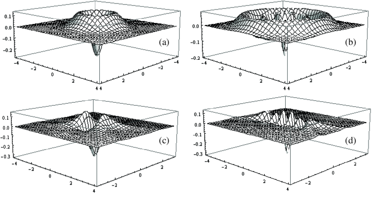
= \displaystyle= ( − 1 ) n e − 2 | α | 2 sech 2 θ π cosh n + 1 2 θ L n ( 4 cosh 2 θ cosh 2 θ | α | 2 ) , superscript 1 𝑛 superscript 𝑒 2 superscript 𝛼 2 sech 2 𝜃 𝜋 superscript 𝑛 1 2 𝜃 subscript 𝐿 𝑛 4 superscript 2 𝜃 2 𝜃 superscript 𝛼 2 \displaystyle\frac{\left(-1\right)^{n}e^{-2\left|\alpha\right|^{2}\text{sech}2\theta}}{\pi\cosh^{n+1}2\theta}L_{n}\left(\frac{4\cosh^{2}\theta}{\cosh 2\theta}\left|\alpha\right|^{2}\right),
a Gaussian-Laguerre type function which may present negative region in phase
space (see Fig.2). In particular, when n = 1 , 𝑛 1 n=1, 34
W 2 ( α ) = − e − 2 | α | 2 sech 2 θ π cosh 2 2 θ ( 1 − 4 cosh 2 θ cosh 2 θ | α | 2 ) . subscript 𝑊 2 𝛼 superscript 𝑒 2 superscript 𝛼 2 sech 2 𝜃 𝜋 superscript 2 2 𝜃 1 4 superscript 2 𝜃 2 𝜃 superscript 𝛼 2 W_{2}\left(\alpha\right)=-\frac{e^{-2\left|\alpha\right|^{2}\text{sech}2\theta}}{\pi\cosh^{2}2\theta}\left(1-\frac{4\cosh^{2}\theta}{\cosh 2\theta}\left|\alpha\right|^{2}\right). (35)
In Fig. 2, the behaviour of WF distributions of photon-added thermo state
are plotted in (q , p 𝑞 𝑝
q,p ( | α | , θ ) 𝛼 𝜃 \left(\left|\alpha\right|,\theta\right) ( | α | , θ ) 𝛼 𝜃 \left(\left|\alpha\right|,\theta\right) θ 𝜃 \theta
Figure 2: Wigner function distributions of photon-added thermo state in (q , p 𝑞 𝑝
q,p θ = 0.2 𝜃 0.2 \theta=0.2 n = 1 𝑛 1 n=1 n = 2 , 𝑛 2 n=2, ( | α | , θ ) 𝛼 𝜃 \left(\left|\alpha\right|,\theta\right) n = 1 𝑛 1 n=1 n = 5 𝑛 5 n=5
VI Wigner function of thermo number state
At finite temperature, according to TFD, the number state | n ⟩ ket 𝑛 \left|n\right\rangle | n , n ~ ⟩ , ket 𝑛 ~ 𝑛
\left|n,\tilde{n}\right\rangle, S ( θ ) | n , n ~ ⟩ 𝑆 𝜃 ket 𝑛 ~ 𝑛
S\left(\theta\right)\left|n,\tilde{n}\right\rangle
| n , n ~ ⟩ = 1 n ! d 2 n d z n d z ~ n | z , z ~ ⟩ | z = z ~ = 0 , ⟨ z ′ | z ⟩ = e z ′ ∗ z , formulae-sequence ket 𝑛 ~ 𝑛
evaluated-at 1 𝑛 superscript 𝑑 2 𝑛 𝑑 superscript 𝑧 𝑛 𝑑 superscript ~ 𝑧 𝑛 ket 𝑧 ~ 𝑧
𝑧 ~ 𝑧 0 inner-product superscript 𝑧 ′ 𝑧 superscript 𝑒 superscript 𝑧 ′ ∗
𝑧 \left|n,\tilde{n}\right\rangle=\frac{1}{n!}\frac{d^{2n}}{dz^{n}d\tilde{z}^{n}}\left.\left|z,\tilde{z}\right\rangle\right|_{z=\tilde{z}=0},\text{\ }\left\langle z^{\prime}\right.\left|z\right\rangle=e^{z^{\prime\ast}z}, (36)
where | z , z ~ ⟩ = exp [ z a † + z ~ a ~ † ] | 0 , 0 ~ ⟩ ket 𝑧 ~ 𝑧
𝑧 superscript 𝑎 † ~ 𝑧 superscript ~ 𝑎 † ket 0 ~ 0
\left|z,\tilde{z}\right\rangle=\exp[za^{{\dagger}}+\tilde{z}\tilde{a}^{{\dagger}}]\left|0,\tilde{0}\right\rangle 19 W 3 ( α ) subscript 𝑊 3 𝛼 W_{3}\left(\alpha\right)
W 3 ( α ) subscript 𝑊 3 𝛼 \displaystyle W_{3}\left(\alpha\right) = \displaystyle= ⟨ n , n ~ | S † Δ ( α ) S | n , n ~ ⟩ quantum-operator-product 𝑛 ~ 𝑛
superscript 𝑆 † Δ 𝛼 𝑆 𝑛 ~ 𝑛
\displaystyle\left\langle n,\tilde{n}\right|S^{{\dagger}}\Delta\left(\alpha\right)S\left|n,\tilde{n}\right\rangle (37)
= \displaystyle= 1 n ! 2 d 2 n d f n d r n d 2 n d z n d t n ⟨ f ∗ , r ∗ | S † Δ ( α ) S | z , t ⟩ | f = r = z = t = 0 evaluated-at 1 superscript 𝑛 2 superscript 𝑑 2 𝑛 𝑑 superscript 𝑓 𝑛 𝑑 superscript 𝑟 𝑛 superscript 𝑑 2 𝑛 𝑑 superscript 𝑧 𝑛 𝑑 superscript 𝑡 𝑛 quantum-operator-product superscript 𝑓 ∗ superscript 𝑟 ∗
superscript 𝑆 † Δ 𝛼 𝑆 𝑧 𝑡
𝑓 𝑟 𝑧 𝑡 0 \displaystyle\frac{1}{n!^{2}}\frac{d^{2n}}{df^{n}dr^{n}}\frac{d^{2n}}{dz^{n}dt^{n}}\left\langle f^{\ast},r^{\ast}\right|S^{{\dagger}}\Delta\left(\alpha\right)S\left.\left|z,t\right\rangle\right|_{f=r=z=t=0}
= \displaystyle= 𝒜 d 2 n d f n d r n d 2 n d z n d t n exp { − ( t z + f r ) tanh 2 θ \displaystyle\mathcal{A}\frac{d^{2n}}{df^{n}dr^{n}}\frac{d^{2n}}{dz^{n}dt^{n}}\exp\left\{-\left(tz+fr\right)\tanh 2\theta\right.
+ ( r t − f z ) sech 2 θ + z E ∗ + f E + r F ∗ + t F } f = r = z = t = 0 , \displaystyle+\left.\left(\allowbreak rt-fz\right)\text{sech}2\theta+zE^{\ast}+fE+r\allowbreak F^{\ast}+\allowbreak tF\right\}_{f=r=z=t=0},
where we have set
𝒜 = e − 2 | α | 2 sech 2 θ π n ! 2 cosh 2 θ , E = 2 α sech 2 θ cosh θ , F = 2 α sech 2 θ sinh θ . formulae-sequence 𝒜 superscript 𝑒 2 superscript 𝛼 2 sech 2 𝜃 𝜋 superscript 𝑛 2 2 𝜃 formulae-sequence 𝐸 2 𝛼 sech 2 𝜃 𝜃 𝐹 2 𝛼 sech 2 𝜃 𝜃 \mathcal{A=}\frac{e^{-2\left|\alpha\right|^{2}\text{sech}2\theta}}{\pi n!^{2}\cosh 2\theta},\text{ }E=2\alpha\text{sech}2\theta\cosh\theta,\text{ \ }F=2\alpha\text{sech}2\theta\allowbreak\sinh\theta. (38)
Expanding the exponential term exp [ ( r t − f z ) sech 2 θ ] 𝑟 𝑡 𝑓 𝑧 sech 2 𝜃 \exp\left[\left(rt-\allowbreak fz\right)\text{sech}2\theta\right]
W 3 ( α ) subscript 𝑊 3 𝛼 \displaystyle W_{3}\left(\alpha\right) = \displaystyle= 𝒜 d 2 n d f n d z n d 2 n d r n d t n exp [ − ( f r + t z ) tanh 2 θ ] 𝒜 superscript 𝑑 2 𝑛 𝑑 superscript 𝑓 𝑛 𝑑 superscript 𝑧 𝑛 superscript 𝑑 2 𝑛 𝑑 superscript 𝑟 𝑛 𝑑 superscript 𝑡 𝑛 𝑓 𝑟 𝑡 𝑧 2 𝜃 \displaystyle\mathcal{A}\frac{d^{2n}}{df^{n}dz^{n}}\frac{d^{2n}}{dr^{n}dt^{n}}\exp\left[-\left(fr+tz\right)\tanh 2\theta\right] (39)
× ∑ l , k = 0 ∞ ( − 1 ) k sech l + k 2 θ l ! k ! ( r t ) l ( f z ) k exp [ z E ∗ + f E + t F + r F ∗ ] z = t = f = r = 0 \displaystyle\times\sum_{l,k=0}^{\infty}\frac{\left(-\allowbreak 1\right)^{k}\text{sech}^{l+k}2\theta}{l!k!}\left(rt\right)^{l}\left(\allowbreak fz\right)^{k}\exp\left[zE^{\ast}+fE+tF\allowbreak+rF^{\ast}\right]_{z=t=f=r=0}
= \displaystyle= 𝒜 ∑ l , k = 0 ∞ ( − 1 ) k sech l + k 2 θ l ! k ! ∂ 2 l ∂ F l ∂ F ∗ l ∂ 2 k ∂ E k ∂ E ∗ k 𝒜 superscript subscript 𝑙 𝑘
0 superscript 1 𝑘 superscript sech 𝑙 𝑘 2 𝜃 𝑙 𝑘 superscript 2 𝑙 superscript 𝐹 𝑙 superscript 𝐹 ∗ absent 𝑙 superscript 2 𝑘 superscript 𝐸 𝑘 superscript 𝐸 ∗ absent 𝑘 \displaystyle\mathcal{A}\sum_{l,k=0}^{\infty}\frac{\left(-\allowbreak 1\right)^{k}\text{sech}^{l+k}2\theta}{l!k!}\frac{\partial^{2l}}{\partial F^{l}\allowbreak\partial F\allowbreak^{\ast l}}\frac{\partial^{2k}}{\partial E^{k}\allowbreak\partial E\allowbreak^{\ast k}}
× d 2 n d f n d z n d 2 n d r n d t n exp [ − ( f r + t z ) tanh 2 θ + f E + r F ∗ + z E ∗ + t F ] z = t = f = r = 0 . \displaystyle\times\frac{d^{2n}}{df^{n}dz^{n}}\frac{d^{2n}}{dr^{n}dt^{n}}\exp\left[-\left(fr+tz\right)\tanh 2\theta+fE\allowbreak+rF^{\ast}+zE^{\ast}+tF\right]_{z=t=f=r=0}.
Then making the variable replacement for f , r , t , z 𝑓 𝑟 𝑡 𝑧
f,r,t,z 39
W 3 ( α ) subscript 𝑊 3 𝛼 \displaystyle W_{3}\left(\alpha\right) = \displaystyle= 𝒜 tanh 2 n 2 θ ∑ l , k = 0 ∞ ( − 1 ) k sech l + k 2 θ l ! k ! ∂ 2 l ∂ F l ∂ F ∗ l ∂ 2 k ∂ E k ∂ E ∗ k 𝒜 superscript 2 𝑛 2 𝜃 superscript subscript 𝑙 𝑘
0 superscript 1 𝑘 superscript sech 𝑙 𝑘 2 𝜃 𝑙 𝑘 superscript 2 𝑙 superscript 𝐹 𝑙 superscript 𝐹 ∗ absent 𝑙 superscript 2 𝑘 superscript 𝐸 𝑘 superscript 𝐸 ∗ absent 𝑘 \displaystyle\mathcal{A}\tanh^{2n}2\theta\sum_{l,k=0}^{\infty}\frac{\left(-\allowbreak 1\right)^{k}\text{sech}^{l+k}2\theta}{l!k!}\frac{\partial^{2l}}{\partial F^{l}\allowbreak\partial F\allowbreak^{\ast l}}\frac{\partial^{2k}}{\partial E^{k}\allowbreak\partial E\allowbreak^{\ast k}} (40)
× d 2 n d f n d r n d 2 n d z n d t n exp [ − f r + f E + r F ∗ tanh 2 θ − t z + z E ∗ + t F tanh 2 θ ] z = t = f = r = 0 \displaystyle\times\frac{d^{2n}}{df^{n}dr^{n}}\frac{d^{2n}}{dz^{n}dt^{n}}\exp\left[-fr+fE\allowbreak+\frac{rF^{\ast}}{\tanh 2\theta}-tz+zE^{\ast}+\frac{tF}{\tanh 2\theta}\right]_{z=t=f=r=0}
= \displaystyle= 𝒜 tanh 2 n 2 θ ∑ l , k = 0 ∞ ( − 1 ) k sech l + k 2 θ l ! k ! 𝒜 superscript 2 𝑛 2 𝜃 superscript subscript 𝑙 𝑘
0 superscript 1 𝑘 superscript sech 𝑙 𝑘 2 𝜃 𝑙 𝑘 \displaystyle\mathcal{A}\tanh^{2n}2\theta\sum_{l,k=0}^{\infty}\frac{\left(-\allowbreak 1\right)^{k}\text{sech}^{l+k}2\theta}{l!k!}
× ∂ k + l ∂ E k ∂ F ∗ l ∂ k + l ∂ E ∗ k ∂ F l H n , n ( E , F ∗ tanh 2 θ ) H n , n ( E ∗ , F tanh 2 θ ) . absent superscript 𝑘 𝑙 superscript 𝐸 𝑘 superscript 𝐹 ∗ absent 𝑙 superscript 𝑘 𝑙 superscript 𝐸 ∗ absent 𝑘 superscript 𝐹 𝑙 subscript 𝐻 𝑛 𝑛
𝐸 superscript 𝐹 ∗ 2 𝜃 subscript 𝐻 𝑛 𝑛
superscript 𝐸 ∗ 𝐹 2 𝜃 \displaystyle\times\frac{\partial^{k+l}}{\partial E^{k}\partial F\allowbreak^{\ast l}}\frac{\partial^{k+l}}{\partial E\allowbreak^{\ast k}\allowbreak\partial F^{l}\allowbreak}H_{n,n}\left(E,\frac{F^{\ast}}{\tanh 2\theta}\right)H_{n,n}\left(E^{\ast},\frac{F}{\tanh 2\theta}\right).
Noticing the formula
∂ l + k ∂ ξ l ∂ η k H m , n ( ξ , η ) = m ! n ! ( m − l ) ! ( n − k ) ! H m − l , n − k ( ξ , η ) , superscript 𝑙 𝑘 superscript 𝜉 𝑙 superscript 𝜂 𝑘 subscript 𝐻 𝑚 𝑛
𝜉 𝜂 𝑚 𝑛 𝑚 𝑙 𝑛 𝑘 subscript 𝐻 𝑚 𝑙 𝑛 𝑘
𝜉 𝜂 \frac{\partial^{l+k}}{\partial\xi^{l}\partial\eta^{k}}H_{m,n}\left(\xi,\eta\right)=\frac{m!n!}{\left(m-l\right)!\left(n-k\right)!}H_{m-l,n-k}\left(\xi,\eta\right), (41)
we have
W 3 ( α ) subscript 𝑊 3 𝛼 \displaystyle W_{3}\left(\alpha\right) = \displaystyle= n ! 2 e − 2 | α | 2 sech 2 θ π cosh 2 θ ∑ l , k = 0 n ( − 1 ) k sech l + k 2 θ tanh 2 ( n − l ) 2 θ l ! k ! [ ( n − l ) ! ( n − k ) ! ] 2 superscript 𝑛 2 superscript 𝑒 2 superscript 𝛼 2 sech 2 𝜃 𝜋 2 𝜃 superscript subscript 𝑙 𝑘
0 𝑛 superscript 1 𝑘 superscript sech 𝑙 𝑘 2 𝜃 superscript 2 𝑛 𝑙 2 𝜃 𝑙 𝑘 superscript delimited-[] 𝑛 𝑙 𝑛 𝑘 2 \displaystyle\frac{n!^{2}e^{-2\left|\alpha\right|^{2}\text{sech}2\theta}}{\pi\cosh 2\theta}\sum_{l,k=0}^{n}\frac{\left(-\allowbreak 1\right)^{k}\text{sech}^{l+k}2\theta\tanh^{2\left(n-l\right)}2\theta}{l!k!\left[\left(n-l\right)!\left(n-k\right)!\right]^{2}} (42)
× | H n − k , n − l ( E , F ∗ tanh 2 θ ) | 2 . absent superscript subscript 𝐻 𝑛 𝑘 𝑛 𝑙
𝐸 superscript 𝐹 ∗ 2 𝜃 2 \displaystyle\times\left|H_{n-k,n-l}\left(E,\frac{F^{\ast}}{\tanh 2\theta}\right)\right|^{2}.
From Eq.(42
In particular, when n = 0 𝑛 0 n=0 tanh θ = e − 1 2 ω β , 𝜃 superscript 𝑒 1 2 𝜔 𝛽 \tanh\theta=e^{-\frac{1}{2}\omega\beta}, cosh 2 θ = 1 1 − e − β ω , sinh 2 θ = e − β ω 1 − e − β ω , formulae-sequence superscript 2 𝜃 1 1 superscript 𝑒 𝛽 𝜔 superscript 2 𝜃 superscript 𝑒 𝛽 𝜔 1 superscript 𝑒 𝛽 𝜔 \cosh^{2}\theta=\frac{1}{1-e^{-\beta\omega}},\sinh^{2}\theta=\frac{e^{-\beta\omega}}{1-e^{-\beta\omega}}, 42 | 0 ( β ) ⟩ ket 0 𝛽 \left|0(\beta)\right\rangle 20 . On the other hand, when T → 0 , → 𝑇 0 T\rightarrow 0, e − β ω → e − ∞ → 0 , → superscript 𝑒 𝛽 𝜔 superscript 𝑒 → 0 e^{-\beta\omega}\rightarrow e^{-\infty}\rightarrow 0, sinh θ → 0 , → 𝜃 0 \sinh\theta\rightarrow 0, cosh θ → 1 , → 𝜃 1 \cosh\theta\rightarrow 1, E → 2 α , → 𝐸 2 𝛼 E\rightarrow 2\alpha, F ∗ tanh 2 θ → α ∗ , → superscript 𝐹 ∗ 2 𝜃 superscript 𝛼 ∗ \frac{F^{\ast}}{\tanh 2\theta}\rightarrow\alpha^{\ast}, 29
H m , n ( ξ , κ ) = ∑ l = 0 min ( m , n ) m ! n ! ( − 1 ) l ξ m − l κ n − l l ! ( n − l ) ! ( m − l ) ! , subscript 𝐻 𝑚 𝑛
𝜉 𝜅 superscript subscript 𝑙 0 𝑚 𝑛 𝑚 𝑛 superscript 1 𝑙 superscript 𝜉 𝑚 𝑙 superscript 𝜅 𝑛 𝑙 𝑙 𝑛 𝑙 𝑚 𝑙 H_{m,n}\left(\xi,\kappa\right)=\sum_{l=0}^{\min(m,n)}\frac{m!n!\left(-1\right)^{l}\xi^{m-l}\kappa^{n-l}}{l!\left(n-l\right)!\left(m-l\right)!}, (43)
which leads to H n − k , 0 ( 2 α , α ∗ ) = ( 2 α ) n − k , subscript 𝐻 𝑛 𝑘 0
2 𝛼 superscript 𝛼 ∗ superscript 2 𝛼 𝑛 𝑘 H_{n-k,0}\left(2\alpha,\alpha^{\ast}\right)=\left(2\alpha\right)^{n-k}, 42
W 3 ( α ) subscript 𝑊 3 𝛼 \displaystyle W_{3}\left(\alpha\right) = \displaystyle= 1 π e − 2 | α | 2 ∑ k = 0 n ( − 1 ) k n ! k ! [ ( n − k ) ! ] 2 | H n − k , 0 ( 2 α , α ∗ ) | 2 1 𝜋 superscript 𝑒 2 superscript 𝛼 2 superscript subscript 𝑘 0 𝑛 superscript 1 𝑘 𝑛 𝑘 superscript delimited-[] 𝑛 𝑘 2 superscript subscript 𝐻 𝑛 𝑘 0
2 𝛼 superscript 𝛼 ∗ 2 \displaystyle\frac{1}{\pi}e^{-2\left|\alpha\right|^{2}}\sum_{k=0}^{n}\frac{\left(-\allowbreak 1\right)^{k}n!}{k!\left[\left(n-k\right)!\right]^{2}}\left|H_{n-k,0}\left(2\alpha,\alpha^{\ast}\right)\right|^{2} (44)
= \displaystyle= ( − 1 ) n π e − 2 | α | 2 ∑ k = 0 n n ! k ! [ ( n − k ) ! ] 2 ( − 4 | α | 2 ) n − k superscript 1 𝑛 𝜋 superscript 𝑒 2 superscript 𝛼 2 superscript subscript 𝑘 0 𝑛 𝑛 𝑘 superscript delimited-[] 𝑛 𝑘 2 superscript 4 superscript 𝛼 2 𝑛 𝑘 \displaystyle\frac{\left(-\allowbreak 1\right)^{n}}{\pi}e^{-2\left|\alpha\right|^{2}}\sum_{k=0}^{n}\frac{n!}{k!\left[\left(n-k\right)!\right]^{2}}\left(-4\left|\alpha\right|^{2}\right)^{n-k}
= \displaystyle= ( − 1 ) n π e − 2 | α | 2 L n ( 4 | α | 2 ) , superscript 1 𝑛 𝜋 superscript 𝑒 2 superscript 𝛼 2 subscript 𝐿 𝑛 4 superscript 𝛼 2 \displaystyle\frac{\left(-\allowbreak 1\right)^{n}}{\pi}e^{-2\left|\alpha\right|^{2}}L_{n}(4\left|\alpha\right|^{2}),
which is just the WF of number state | n ⟩ ket 𝑛 \left|n\right\rangle
In sum, by using TFD and Weyl ordered operators’ order-invariance under
similar transformations, we present a new approach to deriving the exact
expressions of Wigner functions for thermo number state, photon subtracted
and added thermo vacuum state. These WF are related to the Gaussian-Laguerre
type functions, which are easily to be further analysed. The affection of
temperature to nonclassical behaviour of the fields is manifestly shown. For
discussions about the decoherence at finite temperature, we refer to [30,31].
Appendix A Checking Eq.(30
In fact, in original Fock space, the photon-subtracted thermo state is
expressed as [20]
ρ 1 = C 1 Tr a ~ [ a n | 0 ( β ) ⟩ ⟨ 0 ( β ) | a † n ] = C 1 a n ρ c a † n , subscript 𝜌 1 subscript 𝐶 1 subscript Tr ~ 𝑎 delimited-[] superscript 𝑎 𝑛 ket 0 𝛽 bra 0 𝛽 superscript 𝑎 † absent 𝑛 subscript 𝐶 1 superscript 𝑎 𝑛 subscript 𝜌 𝑐 superscript 𝑎 † absent 𝑛 \rho_{1}=C_{1}\text{Tr}_{\tilde{a}}\left[a^{n}\left|0(\beta)\right\rangle\left\langle 0(\beta)\right|a^{{\dagger}n}\right]=C_{1}a^{n}\rho_{c}a^{{\dagger}n}, (A1)
where ρ c subscript 𝜌 𝑐 \rho_{c}
ρ c = ∑ l = 0 ∞ n c l ( n c + 1 ) l + 1 | l ⟩ ⟨ l | = 1 n c + 1 e a † a ln n c n c + 1 , n c = sinh 2 θ . formulae-sequence subscript 𝜌 𝑐 superscript subscript 𝑙 0 superscript subscript 𝑛 𝑐 𝑙 superscript subscript 𝑛 𝑐 1 𝑙 1 ket 𝑙 bra 𝑙 1 subscript 𝑛 𝑐 1 superscript 𝑒 superscript 𝑎 † 𝑎 subscript 𝑛 𝑐 subscript 𝑛 𝑐 1 subscript 𝑛 𝑐 superscript 2 𝜃 \rho_{c}=\sum_{l=0}^{\infty}\frac{n_{c}^{l}}{\left(n_{c}+1\right)^{l+1}}\left|l\right\rangle\left\langle l\right|=\frac{1}{n_{c}+1}e^{a^{{\dagger}}a\ln\frac{n_{c}}{n_{c}+1}},\text{ }n_{c}=\sinh^{2}\theta. (A2)
Using the the coherent state representation of Wigner operator [26],
Δ ( α ) = e 2 | α | 2 ∫ 𝚍 2 z π 2 | z ⟩ ⟨ − z | exp [ − 2 ( z α ∗ − z ∗ α ) ] , Δ 𝛼 superscript 𝑒 2 superscript 𝛼 2 superscript 𝚍 2 𝑧 superscript 𝜋 2 ket 𝑧 bra 𝑧 2 𝑧 superscript 𝛼 ∗ superscript 𝑧 ∗ 𝛼 \Delta\left(\alpha\right)=e^{2\left|\alpha\right|^{2}}\int\frac{\mathtt{d}^{2}z}{\pi^{2}}\left|z\right\rangle\left\langle-z\right|\exp\left[-2\left(z\alpha^{\ast}-z^{\ast}\alpha\right)\right], (A3)
where | z ⟩ ket 𝑧 \left|z\right\rangle
W 1 ( α ) subscript 𝑊 1 𝛼 \displaystyle W_{1}\left(\alpha\right) = Tr ( Δ ( α ) ρ 1 ) absent Tr Δ 𝛼 subscript 𝜌 1 \displaystyle=\text{Tr}\left(\Delta\left(\alpha\right)\rho_{1}\right)
= C 1 e 2 | α | 2 n c + 1 ∫ 𝚍 2 z π 2 ⟨ − z | a n e a † a ln n c n c + 1 a † n | z ⟩ exp [ − 2 ( z α ∗ − z ∗ α ) ] . absent subscript 𝐶 1 superscript 𝑒 2 superscript 𝛼 2 subscript 𝑛 𝑐 1 superscript 𝚍 2 𝑧 superscript 𝜋 2 quantum-operator-product 𝑧 superscript 𝑎 𝑛 superscript 𝑒 superscript 𝑎 † 𝑎 subscript 𝑛 𝑐 subscript 𝑛 𝑐 1 superscript 𝑎 † absent 𝑛 𝑧 2 𝑧 superscript 𝛼 ∗ superscript 𝑧 ∗ 𝛼 \displaystyle=\frac{C_{1}e^{2\left|\alpha\right|^{2}}}{n_{c}+1}\int\frac{\mathtt{d}^{2}z}{\pi^{2}}\left\langle-z\right|a^{n}e^{a^{{\dagger}}a\ln\frac{n_{c}}{n_{c}+1}}a^{{\dagger}n}\left|z\right\rangle\exp\left[-2\left(z\alpha^{\ast}-z^{\ast}\alpha\right)\right]. (A4)
Note that
e a † a ln n c n c + 1 a † n e − a † a ln n c n c + 1 = n c n ( n c + 1 ) n a † n , superscript 𝑒 superscript 𝑎 † 𝑎 subscript 𝑛 𝑐 subscript 𝑛 𝑐 1 superscript 𝑎 † absent 𝑛 superscript 𝑒 superscript 𝑎 † 𝑎 subscript 𝑛 𝑐 subscript 𝑛 𝑐 1 superscript subscript 𝑛 𝑐 𝑛 superscript subscript 𝑛 𝑐 1 𝑛 superscript 𝑎 † absent 𝑛 e^{a^{{\dagger}}a\ln\frac{n_{c}}{n_{c}+1}}a^{{\dagger}n}e^{-a^{{\dagger}}a\ln\frac{n_{c}}{n_{c}+1}}=\frac{n_{c}^{n}}{\left(n_{c}+1\right)^{n}}a^{{\dagger}n}, (A5)
and
e a † a ln n c n c + 1 | z ⟩ = e − 2 n c + 1 2 ( n c + 1 ) 2 | n c z n c + 1 ⟩ , superscript 𝑒 superscript 𝑎 † 𝑎 subscript 𝑛 𝑐 subscript 𝑛 𝑐 1 ket 𝑧 superscript 𝑒 2 subscript 𝑛 𝑐 1 2 superscript subscript 𝑛 𝑐 1 2 ket subscript 𝑛 𝑐 𝑧 subscript 𝑛 𝑐 1 e^{a^{{\dagger}}a\ln\frac{n_{c}}{n_{c}+1}}\left|z\right\rangle=e^{-\frac{2n_{c}+1}{2\left(n_{c}+1\right)^{2}}}\left|\frac{n_{c}z}{n_{c}+1}\right\rangle, (A6)
Eq.(A4) can be rewritten as
W 1 ( α ) subscript 𝑊 1 𝛼 \displaystyle W_{1}\left(\alpha\right) = n c n C 1 e 2 | α | 2 ( n c + 1 ) n + 1 ∫ d 2 z π 2 ⟨ − z | a n a † n | n c z n c + 1 ⟩ absent superscript subscript 𝑛 𝑐 𝑛 subscript 𝐶 1 superscript 𝑒 2 superscript 𝛼 2 superscript subscript 𝑛 𝑐 1 𝑛 1 superscript 𝑑 2 𝑧 superscript 𝜋 2 quantum-operator-product 𝑧 superscript 𝑎 𝑛 superscript 𝑎 † absent 𝑛 subscript 𝑛 𝑐 𝑧 subscript 𝑛 𝑐 1 \displaystyle=\frac{n_{c}^{n}C_{1}e^{2\left|\alpha\right|^{2}}}{\left(n_{c}+1\right)^{n+1}}\int\frac{d^{2}z}{\pi^{2}}\left\langle-z\right|a^{n}a^{{\dagger}n}\left|\frac{n_{c}z}{n_{c}+1}\right\rangle
× exp [ − 2 n c + 1 2 ( n c + 1 ) 2 | z | 2 − 2 ( z α ∗ − z ∗ α ) ] . absent 2 subscript 𝑛 𝑐 1 2 superscript subscript 𝑛 𝑐 1 2 superscript 𝑧 2 2 𝑧 superscript 𝛼 ∗ superscript 𝑧 ∗ 𝛼 \displaystyle\times\exp\left[-\frac{2n_{c}+1}{2\left(n_{c}+1\right)^{2}}\left|z\right|^{2}-2\left(z\alpha^{\ast}-z^{\ast}\alpha\right)\right]. (A7)
Further using the operator identity [29]
a n a † n = ( − 1 ) n : H n , n ( i a † , i a ) : , : superscript 𝑎 𝑛 superscript 𝑎 † absent 𝑛 superscript 1 𝑛 subscript 𝐻 𝑛 𝑛
𝑖 superscript 𝑎 † 𝑖 𝑎 : absent a^{n}a^{{\dagger}n}=\left(-1\right)^{n}\colon H_{n,n}\left(ia^{{\dagger}},ia\right)\colon, (A8)
where H m , n ( x , y ) subscript 𝐻 𝑚 𝑛
𝑥 𝑦 H_{m,n}\left(x,y\right)
H m , n ( x , y ) = ∂ m + n ∂ t m ∂ t ′ n exp [ − t t ′ + t x + t ′ y ] | t = t ′ = 0 , subscript 𝐻 𝑚 𝑛
𝑥 𝑦 evaluated-at superscript 𝑚 𝑛 superscript 𝑡 𝑚 superscript 𝑡 ′ 𝑛
𝑡 superscript 𝑡 ′ 𝑡 𝑥 superscript 𝑡 ′ 𝑦 𝑡 superscript 𝑡 ′ 0 H_{m,n}\left(x,y\right)=\left.\frac{\partial^{m+n}}{\partial t^{m}\partial t^{\prime n}}\exp\left[-tt^{\prime}+tx+t^{\prime}y\right]\right|_{t=t^{\prime}=0}, (A9)
we have
W 1 ( α ) subscript 𝑊 1 𝛼 \displaystyle W_{1}\left(\alpha\right) = ( − 1 ) n e 2 | α | 2 n ! ( n c + 1 ) n + 1 ∂ 2 n ∂ t n ∂ τ n e − t τ absent superscript 1 𝑛 superscript 𝑒 2 superscript 𝛼 2 𝑛 superscript subscript 𝑛 𝑐 1 𝑛 1 superscript 2 𝑛 superscript 𝑡 𝑛 superscript 𝜏 𝑛 superscript 𝑒 𝑡 𝜏 \displaystyle=\frac{\left(-1\right)^{n}e^{2\left|\alpha\right|^{2}}}{n!\left(n_{c}+1\right)^{n+1}}\frac{\partial^{2n}}{\partial t^{n}\partial\tau^{n}}e^{-t\tau}
× ∫ 𝚍 2 z π 2 exp { − 2 n c + 1 n c + 1 | z | 2 + ( i τ n c n c + 1 − 2 α ∗ ) z + ( 2 α − i t ) z ∗ } t = τ = 0 \displaystyle\times\int\frac{\mathtt{d}^{2}z}{\pi^{2}}\exp\left\{-\frac{2n_{c}+1}{n_{c}+1}\left|z\right|^{2}\right.\left.+\left(\frac{i\tau n_{c}}{n_{c}+1}-2\alpha^{\ast}\right)z+\left(2\alpha-it\right)z^{\ast}\right\}_{t=\tau=0}
= ( − 1 ) n n ! π ( n c + 1 ) n e 2 | α | 2 2 n c + 1 ∂ 2 n ∂ t n ∂ τ n exp [ − t τ ] absent superscript 1 𝑛 𝑛 𝜋 superscript subscript 𝑛 𝑐 1 𝑛 superscript 𝑒 2 superscript 𝛼 2 2 subscript 𝑛 𝑐 1 superscript 2 𝑛 superscript 𝑡 𝑛 superscript 𝜏 𝑛 𝑡 𝜏 \displaystyle=\frac{\left(-1\right)^{n}}{n!\pi\left(n_{c}+1\right)^{n}}\frac{e^{2\left|\alpha\right|^{2}}}{2n_{c}+1}\frac{\partial^{2n}}{\partial t^{n}\partial\tau^{n}}\exp\left[-t\tau\right]
exp [ n c + 1 2 n c + 1 ( i τ n c n c + 1 − 2 α ∗ ) ( 2 α − i t ) ] t = τ = 0 \displaystyle\exp\left[\frac{n_{c}+1}{2n_{c}+1}\left(\frac{i\tau n_{c}}{n_{c}+1}-2\alpha^{\ast}\right)\left(2\alpha-it\right)\right]_{t=\tau=0}
= ( − 1 ) n n ! π ( n c + 1 ) n e − 2 | α | 2 2 n c + 1 2 n c + 1 ∂ 2 n ∂ t n ∂ τ n exp { − n c + 1 2 n c + 1 t τ \displaystyle=\frac{\left(-1\right)^{n}}{n!\pi\left(n_{c}+1\right)^{n}}\frac{e^{-\frac{2\left|\alpha\right|^{2}}{2n_{c}+1}}}{2n_{c}+1}\frac{\partial^{2n}}{\partial t^{n}\partial\tau^{n}}\exp\left\{-\frac{n_{c}+1}{2n_{c}+1}t\tau\right.
+ 2 i α ∗ n c + 1 2 n c + 1 t + 2 i α n c 2 n c + 1 τ } t = τ = 0 \displaystyle+\left.2i\alpha^{\ast}\frac{n_{c}+1}{2n_{c}+1}t+2i\alpha\frac{n_{c}}{2n_{c}+1}\tau\right\}_{t=\tau=0}
= e − 2 | α | 2 2 n c + 1 ( 2 n c + 1 ) n + 1 ( − 1 ) n n ! π H n , n ( 2 i n c α ( 2 n c + 1 ) ( n c + 1 ) , 2 i n c + 1 2 n c + 1 α ∗ ) , absent superscript 𝑒 2 superscript 𝛼 2 2 subscript 𝑛 𝑐 1 superscript 2 subscript 𝑛 𝑐 1 𝑛 1 superscript 1 𝑛 𝑛 𝜋 subscript 𝐻 𝑛 𝑛
2 𝑖 subscript 𝑛 𝑐 𝛼 2 subscript 𝑛 𝑐 1 subscript 𝑛 𝑐 1 2 𝑖 subscript 𝑛 𝑐 1 2 subscript 𝑛 𝑐 1 superscript 𝛼 ∗ \displaystyle=\frac{e^{-\frac{2\left|\alpha\right|^{2}}{2n_{c}+1}}}{\left(2n_{c}+1\right)^{n+1}}\frac{\left(-1\right)^{n}}{n!\pi}H_{n,n}\left(\frac{2in_{c}\alpha}{\sqrt{\left(2n_{c}+1\right)\left(n_{c}+1\right)}},2i\sqrt{\frac{n_{c}+1}{2n_{c}+1}}\alpha^{\ast}\right), (A10)
then using the relation
( − 1 ) n n ! H n , n ( x , y ) = L n ( x y ) , superscript 1 𝑛 𝑛 subscript 𝐻 𝑛 𝑛
𝑥 𝑦 subscript 𝐿 𝑛 𝑥 𝑦 \frac{\left(-1\right)^{n}}{n!}H_{n,n}\left(x,y\right)=L_{n}\left(xy\right), (A11)
and noticing that n c = sinh 2 θ , subscript 𝑛 𝑐 superscript 2 𝜃 n_{c}=\sinh^{2}\theta, 2 n c + 1 = cosh 2 θ , 2 subscript 𝑛 𝑐 1 2 𝜃 2n_{c}+1=\cosh 2\theta,
W 1 ( α ) = e − 2 | α | 2 2 n c + 1 π ( 2 n c + 1 ) n + 1 L n ( − 4 n c | α | 2 2 n c + 1 ) , subscript 𝑊 1 𝛼 superscript 𝑒 2 superscript 𝛼 2 2 subscript 𝑛 𝑐 1 𝜋 superscript 2 subscript 𝑛 𝑐 1 𝑛 1 subscript 𝐿 𝑛 4 subscript 𝑛 𝑐 superscript 𝛼 2 2 subscript 𝑛 𝑐 1 W_{1}\left(\alpha\right)=\frac{e^{-\frac{2\left|\alpha\right|^{2}}{2n_{c}+1}}}{\pi\left(2n_{c}+1\right)^{n+1}}L_{n}\left(-\frac{4n_{c}\left|\alpha\right|^{2}}{2n_{c}+1}\right), (A12)
which is just the Eq.(30