Magnetic soliton transport over topological spin texture in chiral helimagnet with strong easy-plane anisotropy

Abstract

We show the existence of an isolated soliton excitation over the topological ground state configuration in chiral helimagnet with the Dzyaloshinskii-Moryia exchange and the strong easy-plane anisotropy. The magnetic field perpendicular to the helical axis stabilizes the kink crystal state which plays a role of ”topological protectorate” for the traveling soliton with a definite handedness. To find new soliton solution, we use the Bäcklund transformation technique. It is pointed out that the traveling soliton carries the magnon density and a magnetic solition transport may be realized.

I Introduction

A study of spatially localized excitations over non-trivial many body ”vacuum” configuration is one of the most challenging problem in condensed matter physics. Of particular interest is a collective transport of observable quantities accompanied with a sliding motion of incommensurate (IC) phase modulation of charge and magnetic degrees of freedom. However, well-known types of sliding density waves such as the charge-density wave and the collinear spin-density-wave cannot easily be observed because the internal phase modulation does not carry directly measured quantity.PWABasicNotions Another example is the charge and spin soliton transport in conjugated polymers where the double degeneracy of ground state configurations gives rise to diffusive solitons.Fukuyama-Takayama In this paper, we demonstrate a new possibility to create an isolated magnetic soliton over the topological ground state configuration in chiral helimagnet with the antisymmetric Dzyaloshinskii-Moryia (DM) exchange and the strong easy-plane anisotropy. We show that the isolated magnetic soliton exists and it can carry the observable magnetic density.

Helimagnetic structures are stabilized by either frustration among exchange couplingsYoshimori59 or the DM relativistic exchange.Dzyaloshinskii58 In the latter case, an absence of the rotoinversion symmetry in chiral crystals causes the Lifshitz invariant in the Landau free energy. Consequently, a long-period incommensurate helimagnetic structure is stabilized with the definite (left-handed or right-handed) chirality fixed by the direction of the DM vector. Over the past two decades, the ground state and linear excitations of the chiral helimagnet under an applied magnetic field have been a subject of extensive studies from both experimental and theoretical viewpoints.Izyumov Concerning nonlinear excitations in this class of spiral systems, the solitonic excitations were studied in the case of easy-axis anisotropy.Borisov It has been revealed that the first simplest soliton solution in the easy-axis helimagnet presents a helical domain wall, a nucleation of a helical phase, whereas the second solution, so-called a wave of rotation, describes a localized change of the phase with a finite velocity, which is accompanied by a coming of moments out of the basal plane (Fig. 1). It turns out that the energy of the wave of rotation is less than that of spin wave with the same linear momentum. In a presence of magnetic field applied along the easy-axis, when a simple helimagnetic structure transforms into the conical one, there are again two solitons with energies less then the energy of spin wave with the same momentum.

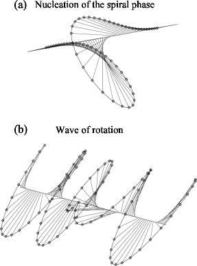
Figure 1: Nonlinear excitations in a helimagnet with an easy axis anisotropy: the nucleation of the spiral phase (a) and the localized wave of rotation (b).

Recent progress on synthesis of new class of helimagnetic structures revives the interest to the case of chiral helimagnet with an easy-plane anisotropy.KIY Findings of solitons in the previous (easy-axis) case was based on a deep analogy between a dynamics of these nonlinear excitations spreading over the easy axis in the chiral helimagnet and a dynamics of nonlinear excitations in the easy-axis ferromagnet. The correspondence reached by a gauge transformation enables to use a well established classification of nonlinear excitations in the last system.Sklyanin However, the theoretical tool turns out to be inappropriate to be applied to the helimagnet with the Lifshitz invariant an the easy-plane anisotropy because the axial symmetry is lost in this case.

In this paper, we show that this problem is resolved with the Bäcklund transformation (BT) technique.Rogers The method we use has been effectively applied to studies of topological vortex-type singular solutions of the elliptic sine-Gordon (SG) equation.Leibbrandt In particular, one- and two-dimensional vortex lattices on both a homogeneous and periodic backgrounds have been constructed using the Bäcklund transformation.Borisov88 One of the main findings of our investigation is an appearance of a non-trivial traveling soliton which carries a localized magnon density. This result may be useful in spintronics technology.Sloncew ; Berger In Sec. II, we describe the model Hamiltonian and basic equations. In Sec. III, we present the method to derive the novel soliton solution by using the Bäcklund transformations. In Sec. IV, we discuss the energy and momentum associated with a creation of the soliton. In Sec. V, we demonstrate that the traveling soliton carries the magnon density. Finally, we summarize the results in Sec. VI.

II Basic equations

We describe the chiral helimagnet by the continuum Hamiltonian density,

$$\mathcal{H} =\frac{\alpha}{2}\left(\frac{\partial\mathbf{M}}{\partial z}\right)^{2}+D\left(M_{x}\frac{\partial M_{y}}{\partial z}-M_{y}\frac{\partial M_{x}}{\partial z}\right)$$

$$+\beta^{2}M_{z}^{2}+h_{x}M_{x},$$ (1)

where the symmetric exchange coupling strength is given by $\alpha>0$, the mono-axial DM coupling strength is given by $D,$ the easy-plane anisotropy strength is given by $\beta^{2}>0$, and the external magnetic field applied perpendicular to the chiral $z$ axis is $\mathbf{h}=(h_{x},0,0).$ When the model Hamiltonian (1) is written, one implicitly assumes that the magnetic atoms form a cubic lattice and the uniform ferromagnetic coupling exists between the adjacent chains to stabilize the long-range order. Then, the Hamiltonian is interpreted as an effective one-dimensional model based on the interchain mean field picture.

Starting with (1), one derives the Landau-Lifshitz equation $\partial\mathbf{M}/\partial t=\left[\mathbf{M}\times\mathbf{H}_{eff}\right]$, where $H_{eff}^{i}=\delta\mathcal{H}/\delta M_{i}$ ($i=x,y,z$) is the effective field acting on the magnetic moment $\mathbf{M}$, the constant $\alpha$ is a feature of the symmetrical exchange coupling. In the explicit form these equations read as

$$\left\{\begin{array}[c]{c}\dfrac{\partial M_{x}}{\partial t}=2\beta^{2}M_{y}M_{z}+2DM_{z}\dfrac{\partial M_{x}}{\partial z}\\ +\alpha M_{z}\dfrac{\partial^{2}M_{y}}{\partial z^{2}}-\alpha M_{y}\dfrac{\partial^{2}M_{z}}{\partial z^{2}},\\ \dfrac{\partial M_{y}}{\partial t}=-2\beta^{2}M_{x}M_{z}+h_{x}M_{z}+2DM_{z}\dfrac{\partial M_{y}}{\partial z}\\ -\alpha M_{z}\dfrac{\partial^{2}M_{x}}{\partial z^{2}}+\alpha M_{x}\dfrac{\partial^{2}M_{z}}{\partial z^{2}},\\ \dfrac{\partial M_{z}}{\partial t}=-h_{x}M_{y}-2DM_{y}\dfrac{\partial M_{y}}{\partial z}-2DM_{x}\dfrac{\partial M_{x}}{\partial z}\\ +\alpha M_{y}\dfrac{\partial^{2}M_{x}}{\partial z^{2}}-\alpha M_{x}\dfrac{\partial^{2}M_{y}}{\partial z^{2}}.\end{array}\right.$$ (2)

By using the polar angles $\theta(z)$ and $\varphi(z)$, we represent $\mathbf{M}(z)=\left(\sin\theta\cos\varphi,\sin\theta\sin\varphi,\cos\theta\right)$ and then Eqs.(2) are transformed into

$$\frac{\partial\theta}{\partial t}=-b\sin\varphi-\cos\theta\left(a+2\frac{\partial\varphi}{\partial z}\right)\frac{\partial\theta}{\partial z}-\sin\theta\frac{\partial^{2}\varphi}{\partial z^{2}},$$ (3)

and

$$\frac{\partial\varphi}{\partial t} =2\beta^{2}\cos\theta-\cos\theta\left(\frac{\partial\varphi}{\partial z}\right)^{2}-b\cos\varphi\cot\theta$$ (4)

$$-a\cos\theta\frac{\partial\varphi}{\partial z}+\frac{1}{\sin\theta}\frac{\partial^{2}\theta}{\partial z^{2}}.$$

Hereinafter, we set $\alpha=1,$ and rewrite $h_{x}=b$, and $D=a/2$. The magnetic kink crystal phase is described by the stationary soliton solution minimizing $\mathcal{H}$ with keeping $\theta=\pi/2$. The solution obeys the SG equation, $\varphi_{zz}=-b\sin\varphi,$ and is given by $\sin(\varphi/2)=\text{sn}(\sqrt{b}z,q),$where $\mathrm{sn}$ is the Jacobi elliptic function with the elliptic modulus $q$ ($0<q^{2}<1$). The magnetic kink crystal phase is sometimes called the soliton lattice (SL) state. The background material behind this solution is summarized in Appendix A. As the modulus $q$ increases, the lattice period of the kink crystal increases and finally diverges at $q\rightarrow 1$, where the incommensurate-to-commensurate (IC-C) phase transition occurs.

Now, our goal is to find out possible nonlinear excitations with small deflections of spins around the basal $xy$ plane. For this purpose we use the expansion

$$\theta(z,t)=\frac{\pi}{2}+\tilde{s}\theta_{1}(z,t)$$ (5)

with the small fluctuation $\theta_{1}\ll 1$ with $\tilde{s}$ being a dummy variable controlling an order of the expansion. Plugging this into Eqs.(3,4), we have

$$0=b\sin\varphi+\tilde{s}\frac{\partial\theta_{1}}{\partial t}+\frac{\partial^{2}\varphi}{\partial z^{2}},$$ (6)

and

$$\frac{\partial\varphi}{\partial t}+\tilde{s}\theta_{1}\left[2\beta^{2}-\left(\frac{\partial\varphi}{\partial z}\right)^{2}-b\cos\varphi-a\frac{\partial\varphi}{\partial z}\right]-\tilde{s}\frac{\partial^{2}\theta_{1}}{\partial z^{2}}=0,$$ (7)

where the terms linear in $\tilde{s}$ are hold.

In real materials,KIY the order of magnitude of the DM coupling gives the long-period wave vector $Q_{0}\approx D\sim 10^{-2}$ and one obtains $\varphi_{z}\approx Q_{0}\sim 10^{-2}$. Magnetic field strength $b$ used in experiment are of order $10^{-5}$. The further analytical treatment is performed in a regime of the strong easy-plane anisotropy, i.e. $\beta^{2}\gtrsim 10^{-3}.$ For spin configurations, where the last term in Eq.(7) may be neglected (see the end of Sec. III), one obtains the relation

$$\theta_{1}=-\frac{1}{2\tilde{s}\beta^{2}}\frac{\partial\varphi}{\partial t},$$ (8)

which establishes a conjugate relation between the dynamical $\theta$ and $\varphi$ variables. The same relation was discussed in the context of soliton dynamics in one-dimensional magnets.Mikeska81 Plugging Eq.(8) into Eq.(6), we have the (1+1)-dimensional SG equation,

$$b\sin\varphi-\frac{1}{2\beta^{2}}\frac{\partial^{2}\varphi}{\partial t^{2}}+\frac{\partial^{2}\varphi}{\partial z^{2}}=0$$ (9)

We use Eqs.(8) and (9) to find the soliton solutions.

III Bäcklund transformation.

The BT is known to be a powerful method to systematically construct non-linear solution in a certain class of partial differential equations. The case of the sine-Gordon equation is briefly summarized in Appendix B. In the new coordinates $\sqrt{2b}\beta t\rightarrow t$, $\sqrt{b}z\rightarrow z$ , two solutions $\varphi$ and $\tilde{\varphi}$ of the SG equation $\varphi_{tt}-\varphi_{zz}=\sin\varphi$ are related via the BT with the real valued parameter $k$.Dodd

$$\left\{\begin{array}[c]{c}\tilde{\varphi}_{t}=\varphi_{z}+k\sin\left(\dfrac{\varphi+\tilde{\varphi}}{2}\right)-\dfrac{1}{k}\sin\left(\dfrac{\varphi-\tilde{\varphi}}{2}\right),\\ \tilde{\varphi}_{z}=\varphi_{t}+k\sin\left(\dfrac{\varphi+\tilde{\varphi}}{2}\right)+\dfrac{1}{k}\sin\left(\dfrac{\varphi-\tilde{\varphi}}{2}\right).\end{array}\right.$$ (10)

We here use the notation $\varphi_{z}=\partial_{z}\varphi=\partial\varphi/\partial z$, $\varphi_{zz}=\partial_{z}^{2}\varphi=\partial^{2}\varphi/\partial z^{2}$, and so on. A pair of the solutions are written in a form,

$$\left\{\begin{array}[c]{c}\varphi\left(z\right)=\pi+4\tan^{-1}\left[F(z)\right],\\ \tilde{\varphi}\left(z,t\right)=\pi+4\tan^{-1}\left[V(z,t)\right].\end{array}\right.$$ (11)

It is easy to verify that the background kink crystal solution, $\sin\left(\varphi/2\right)=\text{sn}\left(z,q\right),$ is reproduced by choosing $F(z)$ as

$$F(z)=\frac{\text{cn}\left(z,q\right)}{1+\text{sn}\left(z,q\right)}.$$ (12)

The dependence of $V$ upon the time and the coordinate should be found through the BT.

To reduce a complexity, it is convenient to rewrite Eqs.(10) in terms of the functions $F$ and $V$. Then, we have the first and the second BTs respectively given by

$$V_{t}=\frac{2kF_{z}+F(k^{2}+1)}{2k(1+F^{2})}V^{2}+\frac{(F^{2}-1)(k^{2}-1)}{2k(1+F^{2})}V$$

$$+\frac{2kF_{z}-F(k^{2}+1)}{2k(1+F^{2})},$$ (13)

and

$$V_{z}=\frac{V\left(F^{2}-1\right)(k^{2}+1)+F(V^{2}-1)(k^{2}-1)}{2k(1+F^{2})}.$$ (14)

The further strategy is straightforward. The time dependence is firstly found from Eq.(13) and then followed by solving of Eq.(14).

III.1 BT Equation (13)

The right-hand side of Eq.(13) is quadratic in $V$. To reach a simplification we use the shift

$$V(z,t)=U(z,t)-\frac{(F^{2}-1)(k^{2}-1)}{2\left(Fk^{2}+2kF_{z}+F\right)}$$ (15)

that transforms Eq.(13) into

$$U_{t}+A(z)U^{2}+B(z)=0,$$ (16)

where

$$A(z)=-\frac{Fk^{2}+2kF_{z}+F}{2k(1+F^{2})},$$ (17)

and

$$B(z) =\left[8k(1+F^{2})\left(Fk^{2}+2kF_{z}+F\right)\right]^{-1}$$

$$\times\left[-16k^{2}F_{z}^{2}+F^{4}(k^{2}-1)^{2}\right.$$

$$\left.+(k^{2}-1)^{2}+2F^{2}(1+k^{4}+6k^{2})\right].$$ (18)

Another simplification is achieved through the identity (see Appendix C),

$$A(z)B(z)=\frac{1}{16}\left(\frac{4}{q^{2}}-k^{2}-\frac{1}{k^{2}}-2\right)=s.$$ (19)

In the sector $s<0$, when the Bäcklund parameter $k$ is constrained by $\left|k+k^{-1}\right|>2/q$, Eq.(16) can be immediately resolved

$$U\left(z,t\right)=\frac{\mathcal{S}}{A(z)}\tanh\left[\frac{\mathcal{S}}{A(z)}\left\{A(z)t-C_{1}(z)\right\}\right],$$ (20)

where $s=-\mathcal{S}^{2}$, and $C_{1}(z)$ is a function of the coordinate. The another sector $s>0$ contains no localized solitons. The time dependence that we need is recovered from Eq.(15)

$$V(z,t) =\frac{\mathcal{S}}{A(z)}\tanh\left[\frac{\mathcal{S}}{A(z)}\left\{A(z)t-C_{1}(z)\right\}\right]$$

$$-\frac{(k^{2}-1)(F^{2}-1)}{2\left(Fk^{2}+2kF_{z}+F\right)}.$$ (21)

III.2 BT Equation (14)

The unknown function $C_{1}(z)$ should be determined from the second BT equation. The derivation is relegated to Appendix D and the result has the form

$$\frac{A_{z}}{A}\left(At-C_{1}\right)-\left(A_{z}t-C_{1z}\right)=\frac{F(k^{2}-1)}{2k(1+F^{2})}.$$ (22)

The substitution $C_{1}(z)=A(z)\mathcal{M}(z)$ transforms this equation into

$$\mathcal{M}_{z}(z)=\frac{F(k^{2}-1)}{2Ak(1+F^{2})}.$$

By using the explicit expressions for $F(z)$ and

$$A(z)=\frac{1}{4k}\left(\frac{2k}{q}\text{dn}\left(z,q\right)-\left(k^{2}+1\right)\text{cn}\left(z,q\right)\right),$$ (23)

one obtain

$$\mathcal{M}_{z}(z)=\frac{(1-k^{2})\,q\,\text{cn}\left(z,q\right)}{(1+k^{2})\,q\,\text{cn}\left(z,q\right)-2k\,\text{dn}\left(z,q\right)}.$$ (24)

After integration, this yields (see Appendix E)

$$\mathcal{M}(z) =\frac{1}{4q{\mathcal{S}}}\log\left|\frac{4{\mathcal{S}}k-(k^{2}-1)\,\text{sn}(z,q)}{4{\mathcal{S}}k+(k^{2}-1)\,\text{sn}(z,q)}\right|-\frac{k^{2}+1}{k^{2}-1}z$$

$$+\frac{4k^{2}(1-q^{2})(1+k^{2})}{(1-k^{2})[(1+k^{2})^{2}q^{2}-4k^{2}]}{\tilde{\Pi}}(n,\text{am}(z,q),q^{2}).$$ (25)

The function $\tilde{\Pi}$ is defined by

$${\tilde{\Pi}}(n,\text{am}(z,q),q^{2})$$

$$=\left\{\begin{array}[c]{c}\Pi(n,\text{am}(z,q),q^{2})\quad\text{for}\quad n<1,\\ -\Pi(N,\text{am}(z,q),q^{2})+\mathcal{F}(\text{am}(z,q),q^{2})\\ +(1/2p_{1})\log\left|\dfrac{\text{cn}(z,q)\text{dn}(z,q)+p_{1}\,\text{sn}(z,q)}{\text{cn}(z,q)\text{dn}(z,q)-p_{1}\,\text{sn}(z,q)}\right|\\ \text{for}\quad n>1,\end{array}\right.$$

where am is the Jacobi elliptic function, and $n={(1-k^{2})^{2}q^{2}}/{[(1+k^{2})^{2}q^{2}-4k^{2}]}$ is the characteristic index of the elliptic integral of the third kind $\Pi$. Furthermore, $N=q^{2}/n$, $p_{1}=\sqrt{(n-1)(1-N)}$, and $\mathcal{F}(...)$ is the elliptic integral of the first kind (see formulas 17.7.7 and 17.7.8 in Ref.AS ). Eqs.(21,23,25) determine explicitly the solution conjugated to the soliton lattice through the Bäcklund transformation. To complete we focus on the asymptotic behavior of the found solution.

For definiteness we choose $|k|>1$, the opposite case $|k|<1$ can be analogously treated. By noting that $\mathcal{M}(z\rightarrow\pm\infty)=\pm\infty$ in this case, and vise versa for $|k|<1$, one obtains

$$V(z \rightarrow\pm\infty,t)\approx\mp\frac{\mathcal{S}}{A(z)}-\frac{(k^{2}-1)(F^{2}-1)}{2\left(Fk^{2}+2kF_{z}+F\right)}$$

$$=\frac{k^{2}-1\pm 4\mathcal{S}k+F^{2}(1-k^{2}\pm 4\mathcal{S}k)}{2\left(Fk^{2}+2kF_{z}+F\right)}$$

$$=q\frac{[(k^{2}-1)\text{sn}(z)\pm 4k\mathcal{S}]}{(1+k^{2})q\,\text{cn}(z)-2k\text{dn}(z)},$$ (26)

if to use the explicit expressions for $F(z)$ and $F_{z}(z)$.

Now, it is easy to prove that Eq.(26) may be rewritten in the form

$$V(z\rightarrow\pm\infty,t)\approx\frac{\text{cn}(z+\delta,q)}{1+\text{sn}(z+\delta,q)},$$ (27)

which is similar to that used for $F(z)$ given by Eq.(12). To find the shift $\delta$ and explicit values of sn$(\delta,q)$, cn$(\delta,q)$, and dn$(\delta,q),$ we use the addition theorems for the elliptic functions,

$$\text{cn}(z+\delta) =\frac{\text{cn}(z)\text{cn}(\delta)-\text{sn}(z)\text{sn}(\delta)\text{dn}(z)\text{dn}(\delta)}{1-q^{2}\text{sn}^{2}(z,q)\text{sn}^{2}(\delta,q)},$$

$$\text{sn}(z+\delta) =\frac{\text{sn}(z)\text{cn}(\delta)\text{dn}(\delta)+\text{sn}(\delta)\text{dn}(z)\text{cn}(z)}{1-q^{2}\text{sn}^{2}(z)\text{sn}^{2}(\delta)},$$

where the elliptic modulus $q$ is omitted. Recalling the periodicity of the form (27) and requiring the function given by Eq.(27) to coincide with the values of Eq.(26) in the boundary points $0$ and $2K$ of the period, we obtain the desired result,

$$\left.\begin{array}[c]{c}\text{sn}(\delta,q)=-\dfrac{2k}{(1+k^{2})q},\\ \text{cn}(\delta,q)=\pm\dfrac{4k\mathcal{S}}{1+k^{2}},\\ \text{dn}(\delta,q)=\dfrac{1-k^{2}}{1+k^{2}}.\end{array}\right.$$ (28)

From this result, we obtain the asymptotic behavior,

$$\tilde{\varphi}\left(z\rightarrow\pm\infty,t\right)\approx\pi+4\tan^{-1}\left[\frac{\text{cn}(z+\delta,q)}{1+\text{sn}(z+\delta,q)}\right],$$

where the sign plus in Eqs.(28) is related with the limit $z\rightarrow\infty$, whereas the minus is did with $z\rightarrow-\infty$. At the end, we note an analogy of the introduced shift $\delta$ with the shift of atoms relative to potential minima in the model of Frank and Van der Merwe (FVdM).Bak Now, we have done everything we need by using BT and found out that the BT creates an additional kink over the background kink crystal state and causes an expansion of the periodical spin structure at infinity.

III.3 The case near the incommensurate-to-commensurate phase boundary

We consider in details the case near the IC-C phase boundary ($q\rightarrow 1$). In this limit, the lattice period of the kink crystal tends to go to infinity and the background state consists of a solitary kink described by $\varphi(z)=2\sin^{-1}\left(\tanh z\right)$. Fortunately, in this limit, Eq. (24) can be integrated by using elementary functions. By using the relationships $\text{cn}\left(z,1\right)=1/\cosh z$, $\text{sn}\left(z,1\right)=\tanh z$ and $\text{dn}\left(z,1\right)=1/\cosh z$, Eq.(24) is integrated to give

$$\mathcal{M}(z)=\frac{1+k}{1-k}z+\mathcal{M}_{0},$$

where $\mathcal{M}_{0}$ is a constant. The same simplifications yield

$$A(z)=-\frac{(k-1)^{2}}{4k\cosh z},$$

and $F_{z}(z,1)=-\left[\cosh z(1+\tanh z)\right]^{-1}$, $F(z,1)=\left[\cosh z(1+\tanh z)\right]^{-1}$. The parameter $\mathcal{S}$ in Eq.(20) reads as $\mathcal{S=}\left(k^{2}-1\right)/\left(4k\right)$ in this case.

After collecting the results together, one eventually obtain

$$V(z,t)=\frac{k+1}{k-1}$$

$$\times\left\{\sinh z+\cosh z\tanh\left[\frac{k^{2}-1}{4k}\left(\frac{1+k}{1-k}z+\mathcal{M}_{0}-t\right)\right]\right\},$$

and

$$\tilde{\varphi}\left(z,t\right)=\pi+4\tan^{-1}\left[V(z,t)\right],$$ (30)

where $\upsilon_{0}=\left(1-k\right)/\left(1+k\right)$ can be thought of as the ”velocity” of the soliton.

The polar angle computed via Eq.(8) takes the form,

$$\theta(z,t) =\frac{\pi}{2}+\sqrt{\frac{b}{2\beta^{2}}}\frac{\left(k+1\right)^{2}}{k}\frac{1}{1+V^{2}}$$

$$\times\frac{\cosh z}{\cosh^{2}\left\{\dfrac{k^{2}-1}{4k}\left(\dfrac{1+k}{1-k}z+\mathcal{M}_{0}-t\right)\right\}}.$$ (31)

This solution is viewed as a ”collision” of two kinks as shown in Fig 2. One of the kinks is ”at rest” as a member of the background configuration, while the other travels with the speed $\upsilon_{0}$ and go through the background without changing its shape.

To justify the inequality $|d^{2}\theta_{1}/dz^{2}|\ll 2\beta^{2}\theta_{1}$ that have been assumed to obtain Eq.(8) the restriction

$$\left|k+\frac{1}{k}\right|\ll 4\beta^{2}$$ (32)

must be fulfilled, which is derived by means of Eq.(31). To obtain this condition, we use the asymptotic of $|(d^{2}\theta_{1}/dz^{2})/\theta_{1}|$ at $z\rightarrow\pm\infty$. Note that the constraint $|k+1/k|>2/q$ excludes only the points $k=\pm 1$. Therefore, there is a region of finite $k$ values provided $\beta^{2}\gg 1/2$.

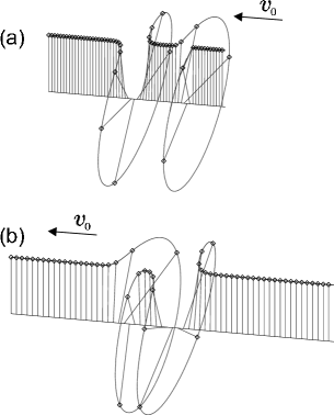
Figure 2: A profile of the soliton excitation at $q\to 1$ in a spiral with an easy plane anisotropy directly before (a) and after (b) ”collision” of the kinks.

IV Energy and momentum

Next we consider the energy and momentum associated with creation of the found soliton. The energy density (1) is written in polar coordinates as

$$\mathcal{H}=\frac{1}{2}\left(\theta_{z}^{2}+\sin^{2}\theta\varphi_{z}^{2}\right)+\frac{a}{2}\sin^{2}\theta\varphi_{z}+\beta^{2}\cos^{2}\theta+b\sin\theta\cos\varphi.$$ (33)

Using the expansion (5,8) and neglecting terms higher than second-order derivatives one obtains

$$\mathcal{H}\approx\frac{1}{2}\varphi_{z}^{2}+\frac{a}{2}\varphi_{z}+\frac{\varphi_{t}^{2}}{4\beta^{2}}+b\cos\varphi\left(1-\frac{\varphi_{t}^{2}}{8\beta^{4}}\right).$$ (34)

In the case of small fields, the term proportional to $b\varphi_{t}^{2}$ may be ignored and the energy density $\mathcal{H}$ measured in $b$ units becomes

$$\mathcal{H}=\cos\varphi+\frac{1}{2}\left(\varphi_{z}^{2}+\varphi_{t}^{2}\right)+c\,\varphi_{z},$$

where $c=a/\left(2\sqrt{b}\right)$ and the coordinates $\sqrt{2b}\beta t\rightarrow t$, $\sqrt{b}z\rightarrow z$ are again used. Following the method suggested in Ref.Kulagin , we find the difference between the energy densities calculated on the solutions coupled by the BT

$$\mathcal{H}(\tilde{\varphi})\mathcal{-H}(\varphi)=c\,\left(\tilde{\varphi}_{z}-\varphi_{z}\right)$$

$$+\frac{1}{k^{2}}\left[k^{2}\sin\left(\frac{\varphi+\tilde{\varphi}}{2}\right)+\sin\left(\frac{\varphi-\tilde{\varphi}}{2}\right)\right]^{2}$$

$$+\left[k\sin\left(\frac{\varphi+\tilde{\varphi}}{2}\right)+\frac{1}{k}\sin\left(\frac{\varphi-\tilde{\varphi}}{2}\right)\right]\varphi_{t}$$

$$+\left[k\sin\left(\frac{\varphi+\tilde{\varphi}}{2}\right)-\frac{1}{k}\sin\left(\frac{\varphi-\tilde{\varphi}}{2}\right)\right]\varphi_{z},$$ (35)

where the transformations (10) are employed. This amounts to a derivative of the function

$$\Psi^{(e)}=c\,\left(\tilde{\varphi}-\varphi\right)+\frac{2}{k}\cos\left(\frac{\varphi-\tilde{\varphi}}{2}\right)-2k\cos\left(\frac{\varphi+\tilde{\varphi}}{2}\right)$$ (36)

with respect to $z$. Thus, the difference of the energies (35) integrated over the total length $L$ of the system is equal to

$$\int\limits_{0}^{L}dz\,\left\{\mathcal{H}(\tilde{\varphi})\mathcal{-H}(\varphi)\right\}=\Psi^{(e)}\left(L\right)-\Psi^{(e)}\left(0\right).$$

The momentum density $\mathcal{P}=\hbar S\left(1-\cos\theta\right)\varphi_{z}$ is treated in the same manner. The spin value $S$ is realted with the magnetic moment by $\textbf{M}=2\mu_{0}\textbf{S}$. Using again the expansions (5,8) and the new coordinates one obtains

$$\mathcal{P}\approx\varphi_{z}-\nu\varphi_{z}\varphi_{t}$$

of the same accuracy as in the case (34). Here, the momentum $\mathcal{P}$ is measured in the units $\hbar S\sqrt{b}$, and $\nu=\sqrt{b/2\beta^{2}}$. The difference between the momentum densities of the solutions conjugated by the BT amounts to

$$\mathcal{P}(\tilde{\varphi})\mathcal{-P}(\varphi)=\Psi_{z}^{(m)},$$

where the function $\Psi^{(m)}$ is given by

$$\Psi^{(m)}=\tilde{\varphi}\mathcal{-}\varphi+\nu\left[\frac{2}{k}\cos\left(\frac{\varphi-\tilde{\varphi}}{2}\right)+2k\cos\left(\frac{\varphi+\tilde{\varphi}}{2}\right)\right].$$ (37)

Therefore, the additional momentum with reference to the background kink crystal state becomes

$$\int\limits_{0}^{L}dz\,\left\{\mathcal{P}(\tilde{\varphi})\mathcal{-P}(\varphi)\right\}=\Psi^{(m)}\left(L\right)-\Psi^{(m)}\left(0\right).$$

V Magnon current.

The magnon current transferred by the $\theta$-fluctuations is determined through the definition of the accumulated magnon density $\mathcal{\rho}_{\text{s}}$ in the total magnon density $\mathcal{N}=g\mu_{\text{B}}S\left(1-\cos\theta\right)$ $=\mathcal{\rho}_{\text{0}}+\mathcal{\rho}_{\text{s}}$, where the ”superfluid” part $\mathcal{\rho}_{\text{s}}=-g\mu_{\text{B}}S\cos\theta$ is conjugated with the magnon time-even current carried by the $\theta$-fluctuations. Then, we obtain the magnon current via the continuity equation $\mathcal{N}_{t}+{J}_{z}^{z}=0$. Here, we compute the magnon current density carried by the traveling soliton in the limit of $q\rightarrow 1$, where the analytical solution with the intrinsic boost transformation  is available based on Eqs.(30) and (31).

The additional magnon density associated with the solutions given by Eqs.(30) and (31) is

$$\delta{\mathcal{N}}=-\frac{S}{2\beta^{2}}\tilde{\varphi}_{t}.$$

Taking the time derivative of $\delta{\mathcal{N}}$ and using the property $\tilde{\varphi}_{t}=-\upsilon_{0}\,\tilde{\varphi}_{z}$ we get $\delta{\mathcal{N}}_{t}=-{J}_{z}^{z}$, where the current ${J}^{z}=S\upsilon_{0}\theta_{1}$ has the explicit form

$${J}^{z}(z,t) =S\sqrt{\frac{b}{2\beta^{2}}}\frac{\left(1-k^{2}\right)}{k}\frac{1}{1+V^{2}}$$

$$\times\frac{\cosh z}{\cosh^{2}\left\{\dfrac{k^{2}-1}{4k}\left(\dfrac{1+k}{1-k}z+\mathcal{M}_{0}-t\right)\right\}}.$$ (38)

Note a significant difference of the result with the magnon current due to the translational motion of the whole kink crystal considered by some of the authors recently.BKO1 In the latter case, the sliding motion of the whole kink crystal excites massive spin wave excitations of the $\theta$-mode above the traveling state that is responsible for a magnon density transport. In the present case, the nontrivial soliton solution itself carries  a localized magnon density (the magnon ”droplet”) due to the intrinsic boost symmetry.

In Fig. 3(a), we depict the background topological charge $\mathcal{Q}=\partial_{z}\varphi$ associated with the standing kink around $z=0$ in the $q\rightarrow 1$ limit, i.e., $\varphi(z)=2\sin^{-1}\left(\text{tanh }z\right)$. In Figs. 3(b-1)-(b-6), we show the magnon density distribution ${J}^{z}(z,t)$ carried by the traveling kink at the time $t=-20,$ $-4,$ $-2,$ $0,$ $2,$ $4,$, respectively, where the soliton travels from left to right. The traveling soliton collides with the standing kink at $t=0$. It is clearly seen that the magnon density is largely amplified when the soliton ”surfs” over the standing kink.

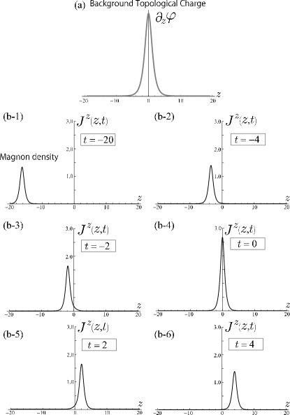
Figure 3: (a) The background topological charge $\mathcal{Q}=\partial_{z}\varphi$ associated with the standing kink. (b-1)-(b-6) The magnon density distribution ${J}^{z}(z,t)$ carried by the traveling kink at the time $t=-20,$ $-4,$ $-2,$ $0,$ $2,$ $4,$ respectively. The soliton travels from left to right. The magnon density is largely amplified when the soliton ”surfs” over the standing kink.

VI Concluding remarks

In summary, by using the Bäcklund transformation technique we investigated soliton excitations in the chiral helimagnetic structure with the antisymmetric Dzyaloshinskii-Moryia exchange and with the strong easy-plane anisotropy, which is experienced by the external magnetic field applied perpendicular to the modulation axis. The soliton we found was obtained as an output of the BT from the kink crystal solution as an input. An essential point is that the traveling soliton cannot exist without the kink crystal (soliton lattice) as a topological background configuration. We may say that the nontrivial topological object is excited over the topological vacuum. The standing kink crystal enables the new soliton to emerge and transport the magnon density. As compared with the motion of the whole kink crystal with a heavy mass,BKO1 our new soliton is a well localized object with a light mass. This object should be certainly, more easily triggered off and propagate over the crystal.

We stress that our soliton has definite chirality, because of the presence of the DM term $D\partial\varphi/\partial z$ in the Hamiltonian density Eq.(1). The presence of this term lifts the degeneracy between the left-handed soliton and the right-handed antisoliton solutions. For example, in Eq.(11), the right-handed antisoliton solutions may be given by changing the sign of the phase gradient, i.e., $\varphi\left(z\right)=\pi-4\tan^{-1}\left[F(z)\right]$, and $\tilde{\varphi}\left(z,t\right)=\pi-4\tan^{-1}\left[V(z,t)\right]$. Although these solutions satisfy the same SG equation as Eq. (9), their static energies are higher than the left-handed soliton solution given by Eq.(11).

Finally, it would be of interest to discuss a difference between the conventional single Bloch wall and our soliton. The Bloch wall is formed within a non-topological background, just a ferromagnet, and it dephases easily. On the other hand, our soliton should be more robust against a dephasing, because it emerges within the topological background (soliton lattice). Chirality and topology support a stability of the moving soliton. This consequence is quite obvious in the context of the soliton theory, but may serve a quite new strategy in the field of spintronics. For example, in the left-handed chiral crystal, only the left-handed kink crystal would be formed and our soliton inherits with the corresponding chirality. Essentially, the crystallographic chirality plays a role of protectorate for the background chiral spin texture and causes the traveling soliton over the background. This new traveling soliton can be regarded as a promising candidate to transport magnetic information by using chiral helimagnet.

Appendix A Formation of the kink crystal state

We here discuss the kink crystal (soliton lattice) formation from a general view point. Let us consider a magnetic system described by the two-component order parameter (OP) ($\eta$, $\xi$) with the Ginzburg-Landau functional,Izyumov

$$\Phi=\frac{1}{L}\int dz\left[r(\eta\xi)+u(\eta\xi)^{2}+w(\eta^{n}+\xi^{n})\right.$$

$$\left.+i\sigma\left(\eta\frac{d\xi}{dz}-\xi\frac{d\eta}{dz}\right)+\gamma\frac{d\eta}{dz}\frac{d\xi}{dz}\right],$$ (39)

where the condition $u>0$, $\gamma>0$ ensures a stability of extremal points of the functional. The signs of $w$ and $\sigma$ are arbitrary. We assume the spin arrangement is uniform in the $x$ and $y$ directions and hence the volume integral is implicitly reduced to one-dimensional integration over $z$-axis, where $L$ is a crystal size in this direction. In the approximation of constant OP modulus, $\rho=\text{const}$, when $\eta=\rho e^{i\varphi}$ and $\xi=\rho e^{-i\varphi}$, the functional (39) depends only on the phase $\varphi,$

$$\Phi =r\rho^{2}+u\rho^{4}$$

$$+\frac{1}{L}\int dz\left\{\gamma\rho^{2}\left(\frac{d\varphi}{dz}\right)^{2}+2\sigma\rho^{2}\frac{d\varphi}{dz}+2w\rho^{n}\cos(n\varphi)\right\},$$ (40)

and includes $\rho$ as a parameter. Minimization of $\Phi$ with respect to $\varphi$ results in the equation

$$\frac{d^{2}}{dz^{2}}(n\varphi)+v\sin(n\varphi)=0,$$ (41)

where the effective anisotropy parameter is defined by $v=n^{2}(w/\gamma)\rho^{(n-2)}$. The case of magnetic field corresponds to $n=1$.

Without of the nonlinear anisotropy term, Eq.(41) is resolved by $\varphi=Qz$ which describes an one-harmonic IC structure, for example, a simple helimagnet, with the wave vector $Q=-\sigma/\gamma$. At finite $v,$ the exact periodic solution is given by

$$\sin\left[\frac{n}{2}\varphi(z)\right]=\text{sn}\left(\frac{\sqrt{v}}{q}z,q\right).$$ (42)

The elliptic modulus $q$ must be determined by minimizing the corresponding energy,

$$\Phi_{\text{IC}} =r\rho^{2}+u\rho^{4}-2\rho^{2}|\sigma|\frac{\pi\sqrt{v}}{nqK}$$

$$+2\rho^{2}\gamma\frac{v}{n^{2}}\left(\frac{q-2}{q^{2}}+\frac{4}{q^{2}}\frac{E}{K}\right),$$ (43)

where $K$ and $E$ denote the elliptic integrals of the first and second kind, respectively. This procedure yields $q$ as a function of the anisotropy parameter $v$,

$$E/q=\sqrt{v_{c}/v},$$ (44)

with the critical anisotropy parameter being defined by $v_{c}=n^{2}\pi^{2}\sigma^{2}/16\gamma^{2}.$ A change of $q$ from 0 to 1 corresponds to a change of $v$ from 0 to $v_{c}$. Varying the parameter $v$ causes a drastic change in the behavior of the amplitude (42). The region of an almost constant phase within the period $l$ comes up at $v\rightarrow v_{c}$, while the phase rapidly changes at the ends of the period, where the overall phase change is $2\pi/n$. The region of the constant phase increases as $v\rightarrow v_{c}$. For $0<v<v_{c}$, the kink crystal phase is stabilized, where a periodic array of C-phase regions separated by the kinks (solitons). The spatial period is given by $l=4qK/\sqrt{v}$, and it diverges logarithmically at $v\rightarrow v_{c}$, i.e. $q\rightarrow 1$,

$$l=(4q/\sqrt{v})\ln[4/\sqrt{1-q^{2}}].$$ (45)

Appendix B Bäcklund transformation

An existence of exact multi-soliton solutions is a peculiar property of the SG equation, and the BT is a systematic way to obtain them. Indeed, let both $\varphi_{0}$ and $\varphi_{1}$ are solutions of the SG equation

$$\partial_{+}\partial_{-}\varphi=\sin\varphi$$

written via light-cone coordinates $x^{+}=\left(x+t\right)/2$, and $x^{-}=\left(x-t\right)/2$. Then, the Bäcklund transformation $\varphi_{1}=\mathcal{B}_{a}\left[\varphi_{0}\right]$ is given by

$$\partial_{\pm}\left(\dfrac{\varphi_{1}\mp\varphi_{0}}{2}\right)=e^{\pm\lambda}\sin\left(\dfrac{\varphi_{1}\pm\varphi_{0}}{2}\right),$$ (46)

where $a=e^{\lambda}$ is called a scale parameter. The relation is consistent with the SG equation, i.e., $\partial_{-}\partial_{+}\varphi_{0}=\sin\varphi_{0}$ and $\partial_{-}\partial_{+}\varphi_{1}=\sin\varphi_{1}$. Any two functions $\varphi_{0}$ and $\varphi_{1}$ that satisfy the BT necessarily solve the SG equation. Eq.(46) is nothing but Eq. (10).

It turns out that analytical expression for multi-soliton solutions may be outlined by an entirely algebraic procedure because the BT embodies a nonlinear superposition principle known as Bianchi’s permutation theorem. Suppose that $\varphi_{0}$ is a seed SG solution, and $\varphi_{1,2}$ are the BTs of $\varphi_{0}$, i.e.

$$\varphi_{1}=\mathcal{B}_{a_{1}}\left[\varphi_{0}\right],\quad\varphi_{2}=\mathcal{B}_{a_{2}}\left[\varphi_{0}\right].$$

Two successive BTs commute, i.e. $\mathcal{B}_{a_{1}}\mathcal{B}_{a_{2}}=\mathcal{B}_{a_{2}}\mathcal{B}_{a_{1}}$, if the Bianchi’s identity

$$\varphi_{3}=\varphi_{0}+4\tan^{-1}\left[\dfrac{a_{2}+a_{1}}{a_{2}-a_{1}}\tan\left(\dfrac{\varphi_{2}-\varphi_{1}}{4}\right)\right]$$

is fulfilled. It means that the non-linear superposition rule holds $\varphi_{3}=\mathcal{B}_{a2}\left[\varphi_{1}\right]$, $\varphi_{3}=\mathcal{B}_{a1}\left[\varphi_{2}\right]$. This algebraic relation indicates that a series of soliton solutions is given by $\varphi=4\tan^{-1}\left[f/g\right]$, which supports the forms of Eq.(11).

Appendix C Computation of the product $A(z)B(z)$

Our objective is to find the product $A(z)B(z)$. By using Eqs.(17,18) we obtain

$$A(z)B(z)$$

$$=\frac{1}{16k^{2}(1+F^{2})^{2}}$$

$$\times\left[16k^{2}F_{z}^{2}-F^{4}(k^{2}-1)^{2}-(k^{2}-1)^{2}-2F^{2}(1+k^{4}+6k^{2})\right]$$

$$=\frac{1}{16k^{2}(1+F^{2})^{2}}$$

$$\times\left[16k^{2}F_{z}^{2}-4F^{2}(k^{2}+1)^{2}-\left(F^{2}-1\right)^{2}\left(k^{2}-1\right)^{2}\right].$$ (47)

The function $F(z)$ has the derivative

$$F_{z}(z)=-\frac{1}{q}\frac{\text{dn}(z,q)}{1+\text{sn}(z,q)},$$

that yields for the numerator in Eq.(47)

$$16k^{2}F_{z}^{2}-4F^{2}(k^{2}+1)^{2}-\left(F^{2}-1\right)^{2}\left(k^{2}-1\right)^{2}$$

$$=16\frac{k^{2}}{q^{2}}\frac{\text{dn}^{2}(z,q)}{\left(1+\text{sn}(z,q)\right)^{2}}-4(k^{2}+1)^{2}\frac{\text{cn}^{2}(z,q)}{\left(1+\text{sn}(z,q)\right)^{2}}$$

$$-4(k^{2}-1)^{2}\frac{\text{sn}^{2}(z,q)}{\left(1+\text{sn}(z,q)\right)^{2}}$$

$$=\frac{4}{\left(1+\text{sn}(z,q)\right)^{2}}\left(\frac{4k^{2}}{q^{2}}-k^{4}-1-2k^{2}\right).$$ (48)

Thus, we reproduce the result (19). Note that the product $A(z)B(z)$ embodies no coordinate dependence, hence it equals a constant $s$.

Appendix D Derivation of Eq.(22)

To derive the determining equation for the function $C_{1}(z)$ we rewrite Eq.(14) through the function $U\left(z,t\right)$

$$U_{z}=\frac{FF_{z}(k^{2}-1)}{Fk^{2}+2F_{z}k+F}$$

$$-\frac{(k^{2}-1)(F^{2}-1)\left(F_{z}k^{2}+2F_{zz}k+F_{z}\right)}{2\left(Fk^{2}+2F_{z}k+F\right)^{2}}$$

$$+\frac{F^{2}(k^{2}+1)}{2k(1+F^{2})}\left(U-\frac{(k^{2}-1)(F^{2}-1)}{2\left(Fk^{2}+2kF_{z}+F\right)}\right)$$

$$-\frac{(k^{2}+1)}{2k(1+F^{2})}\left(U-\frac{(k^{2}-1)(F^{2}-1)}{2\left(Fk^{2}+2kF_{z}+F\right)}\right)$$

$$+\frac{F(k^{2}-1)}{2k(1+F^{2})}\left[\left(U-\frac{(k^{2}-1)(F^{2}-1)}{2\left(Fk^{2}+2kF_{z}+F\right)}\right)^{2}-1\right],$$

and use Eq.(20) to obtain the relation,

$$\frac{\mathcal{S}}{A}\left[\frac{F^{2}(k^{2}+1)}{2k(1+F^{2})}+\frac{A_{z}}{A}-\frac{(k^{2}+1)}{2k(1+F^{2})}\right.$$

$$\left.-\frac{F(k^{2}-1)}{2k(1+F^{2})}\frac{(k^{2}-1)(F^{2}-1)}{\left(Fk^{2}+2kF_{z}+F\right)}\right]\tanh(T)$$

$$+\left(\frac{\mathcal{S}}{A}\right)^{2}\frac{1}{\cosh^{2}\left(T\right)}$$

$$\times\left[\frac{A_{z}}{A}\left(At-C_{1}\right)-\left(A_{z}t-C_{1z}\right)-\frac{F(k^{2}-1)}{2k(1+F^{2})}\right]$$

$$-\frac{(k^{2}+1)(k^{2}-1)(F^{2}-1)^{2}}{4k(1+F^{2})\left(Fk^{2}+2kF_{z}+F\right)}$$

$$+\frac{(k^{2}-1)FF_{z}}{Fk^{2}+2kF_{z}+F}-\frac{(k^{2}-1)F}{2k(1+F^{2})}$$

$$+\left(\frac{\mathcal{S}}{A}\right)^{2}\frac{(k^{2}-1)F}{2k(1+F^{2})}$$

$$-\frac{(k^{2}-1)(F^{2}-1)\left(F_{z}k^{2}+2kF_{zz}+F_{z}\right)}{2\left(Fk^{2}+2kF_{z}+F\right)^{2}}$$

$$+\frac{(k^{2}-1)^{3}F(F^{2}-1)^{2}}{8k(F^{2}+1)\left(Fk^{2}+2kF_{z}+F\right)^{2}}$$

$$=0,$$ (49)

where $T=\left(\mathcal{S}/A\right)\left(At-C_{1}\right)$. Being constant at any time moment, Eq.(49) means that the coefficients before $\tanh(T)$ and $\cosh^{-2}\left(T\right)$ turn simultaneously into zero. With some tedious but a straightforward algebra (see below) one finds that only the factor before $\cosh^{-2}\left(T\right)$ produces the non-trivial result (22).

Indeed, consider the coefficient before $\tanh(T)$ in Eq.(49)

$$\frac{\mathcal{S}}{A}\left[\frac{F^{2}(k^{2}+1)}{2k(1+F^{2})}+\frac{A_{z}}{A}-\frac{(k^{2}+1)}{2k(1+F^{2})}\right.$$

$$\left.-\frac{F(k^{2}-1)}{2k(1+F^{2})}\frac{(k^{2}-1)(F^{2}-1)}{\left(Fk^{2}+2kF_{z}+F\right)}\right]$$

$$=\frac{\mathcal{S}}{2kA^{2}(1+F^{2})\left(Fk^{2}+2kF_{z}+F\right)}$$

$$\times\left[F(k^{2}-1)^{2}(F^{2}-1)A\right.$$

$$-2kA_{z}(1+F^{2})\left(F\left(k^{2}+1\right)+2kF_{z}\right)$$

$$\left.+A(k^{2}+1)(1-F^{2})\left(F\left(k^{2}+1\right)+2kF_{z}\right)\right]$$

$$=\frac{\mathcal{S}}{A^{2}(1+F^{2})\left(Fk^{2}+2kF_{z}+F\right)}$$

$$\times\left[A(1-F^{2})\left(2kF+F_{z}(k^{2}+1)\right)\right.$$

$$\left.-A_{z}(1+F^{2})\left(F\left(k^{2}+1\right)+2kF_{z}\right)\right].$$ (50)

Now we use Eq.(17) to find

$$\frac{A_{z}}{A}=\frac{1}{1+F^{2}}\frac{1}{F\left(k^{2}+1\right)+2kF_{z}}$$

$$\times\left[2kF_{zz}(1+F^{2})+\left(k^{2}+1\right)F_{z}(1+F^{2})\right.$$

$$\left.-4kFF_{z}^{2}-2F^{2}F_{z}\left(k^{2}+1\right)\right].$$ (51)

The function $F(z)$ obeys the equation

$$(1+F^{2})F_{zz}-2FF_{z}^{2}=-F(F^{2}-1),$$

which is derived from the SG equation (9). Together with Eq.(51) this produces

$$\frac{A_{z}}{A}=\frac{1-F^{2}}{1+F^{2}}\frac{F_{z}\left(k^{2}+1\right)+2kF}{F\left(k^{2}+1\right)+2kF_{z}}.$$

Plugging this into the right-hand side of Eq.(50) we come to zero.

After lengthy manipulation it may be shown that the free terms in Eq.(49), i.e. those without either $\tanh(T)$ or $\cosh^{-2}\left(T\right)$ factors, are simplified to

$$-\left(k^{2}-1\right)\left[q^{2}k^{4}-2k^{2}q^{2}(8\mathcal{S}^{2}-1)-4k^{2}+q^{2}\right]$$

$$\times\text{cn}\left(z,q\right)\,\frac{\left[\left(k^{2}+1\right)q\,\text{cn}\left(z,q\right)-2k\,\text{dn}\left(z,q\right)\right]^{3}}{16k^{3}q^{5}\left[1+\text{sn}\left(z,q\right)\right]^{3}}.$$

The factor $q^{2}k^{4}-2k^{2}q^{2}(8\mathcal{S}^{2}-1)-4k^{2}+q^{2}$ equals to zero bearing in mind Eq.(19).

Appendix E Derivation of Eq.(25)

To obtain $\mathcal{M}(z),$ the derivative (24) is split into two parts,

$$\mathcal{M}_{z}(z)=\mathcal{M}_{0}(z)+\mathcal{M}_{1}(z),$$

where

$$\mathcal{M}_{0}(z) =\frac{(1-k^{4})q^{2}\text{cn}^{2}(z,q)}{(1+k^{2})^{2}q^{2}-4k^{2}-(1-k^{2})^{2}q^{2}\text{sn}^{2}(z,q)},$$

$$\mathcal{M}_{1}(z) =\frac{2kq(1-k^{2})\text{cn}(z,q)\text{dn}(z,q)}{(1+k^{2})^{2}q^{2}-4k^{2}-(1-k^{2})^{2}q^{2}\text{sn}^{2}(z,q)},$$

and both terms are separately considered.

The integration of $\mathcal{M}_{0}(z)$ is straightforwardly performed and one obtains

$$\int dz\,\mathcal{M}_{0}(z)$$

$$=-\frac{k^{2}+1}{k^{2}-1}z+\frac{4k^{2}(1-q^{2})(1+k^{2})}{(1-k^{2})[(1+k^{2})^{2}q^{2}-4k^{2}]}$$

$$\times\Pi\left(\frac{(1-k^{2})^{2}q^{2}}{(1+k^{2})^{2}q^{2}-4k^{2}},\text{am}(z,q),q^{2}\right),$$

where

$$\Pi(u,a,q^{2})=\int_{0}^{u}\frac{q^{2}\text{sn}(a,q)\text{cn}(a,q)\text{dn}(a,q)\text{sn}^{2}(u,q)}{1-q^{2}\text{sn}^{2}(a,q)\text{sn}^{2}(u,q)}\,du$$

is the elliptical integral of the third kind.

Taking into account the relationships $(1+k^{2})^{2}q^{2}-4k^{2}=16q^{2}k^{2}{\mathcal{S}}^{2}$ and $\text{cn}(z,q)\text{dn}(z,q)=({d}/{dz}){\text{sn}(z,q)}$ the second term can be written as follows

$$\mathcal{M}_{1}(z) =\frac{(1-k^{2})}{4{\mathcal{S}}}\left[\frac{1}{4{\mathcal{S}}qk-(1-k^{2})q\text{sn}(z,q)}\right.$$

$$\left.+\frac{1}{4{\mathcal{S}}qk+(1-k^{2})q\text{sn}(z,q)}\right]\frac{d}{dz}\text{sn}(z,q)$$

that yields the desired result

$$\int dz\,\mathcal{M}_{1}(z)=\frac{1}{4q{\mathcal{S}}}\log\left|\frac{4{\mathcal{S}}k-(k^{2}-1)\,\text{sn}(z,q)}{4{\mathcal{S}}k+(k^{2}-1)\,\text{sn}(z,q)}\right|.$$

References

• (1) P. W. Anderson, Basic Notions of Condensed Matter Physics, Section 4E, Benjamin/Cummings, Advanced Book Program, California, 1984.
• (2) For example, H. Fukuyama and H. Takayama, in Electronic Properties of Inorganic Quasi-One-Dimensional Materials, I, edited by P. Monceau (Reidel, Dordrecht, 1985), p. 41.
• (3) A. Yoshimori, J. Phys. Soc. Jpn. 14, 807 (1959).
• (4) I. E. Dzyaloshinskii, J. Phys. Chem. Solids 4, 241 (1958); Sov. Phys. JETP 19, 960 (1964); Sov. Phys. JETP 20, 665 (1965).
• (5) Yu.A. Izyumov, Sov. Phys. Usp. 27, 845 (1984).
• (6) A.B. Borisov, Yu.A. Izyumov, Dokl. Akad. Nauk SSSR 283, 859 (1985).
• (7) J. Kishine, K. Inoue, and Y. Yoshida: Prog. Theoret. Phys., Supplement 159, 82 (2005).
• (8) H. J. Mikeska, J. Appl. Phys. 52, 1950 (1981).
• (9) E.K. Sklyanin, ”On the complete integrability of the Landau-Lifshitz equation” (in Russian), Preprint LOMI, Leningrad E-3-79,Leningrad, 1979.
• (10) C. Rogers, W.K. Schief, Bäcklund and Darboux transformations: geometry and modern applications in soliton theory. Cambridge Uiniversity Press, 2002.
• (11) G. Leibbrandt, Phys. Rev. B 15, 3353 (1977).
• (12) A.B. Borisov and VV. Kiselev, Physica D 31, 49 (1988).
• (13) J.C. Sloncewski, J. Magn.Magn. Mater. 159, L1 (1996).
• (14) L. Berger, Phys. Rev. B 54, 9553 (1996).
• (15) R.K. Dodd, and R.K. Bullough, Proc. R. Soc.Lond. A 351, 499 (1976).
• (16) M. Abramowitz, and I. Stegun, Handbook of Mathematical Functions (Chapter 17). Dover Publications Inc., New York, 1965.
• (17) P. Bak, Rep. Prog. Phys. 45, 587 (1982).
• (18) N.E. Kulagin (private communication).
• (19) I.G. Bostrem, J. Kishine, A.S. Ovchinnikov, Phys. Rev. B 77, 132405 (2008); ibid. 78, 064123 (2008).