Understanding light scalar meson by color-magnetic wavefunction in QCD sum rule

Abstract

In this paper, we study the $0^{+}$ nonet mesons as tetraquark states with interpolating currents induced from the color-magnetic wavefunction. This wavefunction is the eigenfunction of effective color-magnetic Hamiltonian with the lowest eigenvalue, meaning that the state depicted by this wavefunction is the most stable one and is most probable to be observed in experiments. Our approach can be recognized as determining interpolating currents dynamically. We perform an OPE calculation up to dimension eight condensates and find that the best QCD sum rule is achived when the current induced from the color-magnetic wavefunction is a proper mixture of the tensor and pseudoscalar diquark-antidiquark bound states. Compared with previous results, to sigma(600) and kappa(800), our results appear better, due to larger pole contribution. The direct instanton contribution are also considered, which yields a consistent result with previous OPE results. Finally, we also discuss the $\eta^{\prime}$ problem as a possible six-quark state.

I Introduction

In past decades, the question how to validly interpret scalar mesons with their mass below 1 GeV stimulated many discussions and controversies amsler . In the naive constituent quark model, they are expected to be $SU(3)_{f}$ nonet consisting of a quark and an antiquark, with one unit of orbital excitation for positive parity. However, due to the fact that the orbital excitation contributes energy about 0.5 GeV, it is difficult to interpret their light mass as well as their mass spectrum jaffe1 . Moreover, $a_{0}(980)$ and $f_{0}(980)$ couple to $K\bar{K}$ channel strongly, which is in contradictory to the prediction by naive $q\bar{q}$ mesons picture. This situation very naturally leads to alternative interpretation about these mesons, such as tetraquark states jaffe2 ; maiani ; brito ; wang ; zhu1 ; zhu2 ; zhu3 ; zhu4 ; lee1 ; lee2 ; lee3 ; lee4 ; Kojo ; Matheus ; Zhang ; Latorre , which were put forward many years ago in jaffe3 ; jaffe4 . Recently, ’t Hooft et. al. thooft and authors of schechter found out new evidence from the instanton induced effective Lagrangian, implying that the predominant component of light scalar meson is tetraquark.

In 1977, using the MIT bag model jaffe5 , Jaffe suggested the existence of a light scalar nonet with masses below 1 GeV jaffe3 ; jaffe4 . This nonet is composed by bound states of diquark and antidiquark. The dominant interaction generating the bound state is from one-gluon exchange which induces the following effective Hamiltonian

$$H_{eff}=-\widetilde{C}\sum_{i\neq j}(\lambda_{i}\cdot\lambda_{j})(\overrightarrow{\sigma}_{i}\cdot\overrightarrow{\sigma}_{j}),$$ (1)

where $\widetilde{C}>0$ is the strength factor constant, $\overrightarrow{\sigma}_{i}$ and $\lambda_{i}$ are $2\times 2$ Pauli matrices and $3\times 3$ Gell-Mann color operators for the $i$th quark. This is a simple generalization of the Breit spin-spin interaction to include a similar color-color piece. It is also known as “color-magnetic” or “color-spin” interaction of QCD, which was first discussed in the pioneering work of De Rujula, Georgi, Glashow DGG . Hereafter, we will call the eigenstates of $H_{eff}$ as color-magnetic eigenstates. The eigenfunctions and corresponding eigenvalues of $H_{eff}$ for $q^{2}\bar{q}^{2}$ system (tetraquark) have been presented in jaffe3 ; jaffe4 . In these work, the eigenstate with the largest mass defect is

$$|0^{+},\underline{9}\rangle=0.972\;|0^{+}\underline{9}[1]\rangle+0.233\;|0^{+}\underline{9}[405]\rangle,$$ (2)

with

$$H_{eff}|0^{+},\underline{9}\rangle=-43.36\widetilde{C}|0^{+},\underline{9}\rangle.$$ (3)

where $0^{+}$ stands for the $J^{P}$, $\underline{9}$ denotes flavor $SU(3)_{f}$-nonet, and $\underline{9}[1]$ ($\underline{9}[405]$) represents the nonet belonging to $[1]$-representation ($[405]$-representation) of color-spin $SU(6)_{CS}$. Explicitly, they are

$$|0^{+}\underline{9}[1]\rangle = \sqrt{6\over 7}|(6,3)\underline{\bar{3}};\;(\bar{6},\bar{3})\underline{3};\;(1,1)\rangle+\sqrt{1\over 7}|(\bar{3},1)\underline{\bar{3}};\;(3,1)\underline{3};\;(1,1)\rangle,$$ (4)

$$|0^{+}\underline{9}[405]\rangle = \sqrt{1\over 7}|(6,3)\underline{\bar{3}};\;(\bar{6},\bar{3})\underline{3};\;(1,1)\rangle-\sqrt{6\over 7}|(\bar{3},1)\underline{\bar{3}};\;(3,1)\underline{3};\;(1,1)\rangle.$$ (5)

In the right hand side of above equations, there is state of $|(6,3)\underline{\bar{3}};\;(\bar{6},\bar{3})\underline{3};\;(1,1)\rangle$, where $(6,3)\underline{\bar{3}}$ indicates that the diquark is in 6-dimension symmetric representation of color $SU(3)_{C}$ with spin $S=1$ (so $2S+1=3$), and in 3-dimension $\bar{3}$ representation of flavor $SU(3)_{f}$. While $(\bar{6},\bar{3})\underline{3}$ means the antidiquark is in the conjugate representation. And (1,1) means the bound state of diquark and antidiquark is singlet both in color and spin. In the following, without ambiguity, the diquark and antidiquark will be denoted according to their $SU(3)_{C}$ representations. For example, $\mathbf{6_{c}}$ diquark signifies the diquark’s wavefunction is $(6,3)\underline{\bar{3}}$. Similarly, $|(\bar{3},1)\underline{\bar{3}};\;(3,1)\underline{3};\;(1,1)\rangle$ is comprised of spin-0 $\mathbf{\bar{3}_{c}}$ diquark and $\mathbf{3_{c}}$ antidiquark.

Basing on Eq. (3), Jaffe claimed that the scalar tetraquarks with masses below 1GeV exist and the color-spin part of their wavefunctions can be described by $|0^{+}\underline{9}\rangle$. Utilizing the latest data, Jaffe’s statement could be roughly checked for a visual comprehension. For instance, a data fit of charmed baryons determines the constituent quark masses hogaasen1 ; hogaasen2 ; dy :

$$m^{c}_{u}\approx m^{c}_{d}\approx 360{\rm MeV}\leavevmode\nobreak\ \leavevmode\nobreak\ \leavevmode\nobreak\ m^{c}_{s}\approx 540{\rm MeV},$$ (6)

where $c$ is the abbreviation of “constituent”. The strength factor constants related to the light quarks are

$$\widetilde{C} \approx \widetilde{C}_{qq}\approx 20{\rm MeV},\leavevmode\nobreak\ \leavevmode\nobreak\ \leavevmode\nobreak\ \leavevmode\nobreak\ \leavevmode\nobreak\ {\rm with}\;\;q\in\{u,d\},$$ (7)

$$(\widetilde{C}_{qs} = 15{\rm MeV},\leavevmode\nobreak\ \leavevmode\nobreak\ \leavevmode\nobreak\ \widetilde{C}_{ss}=10{\rm MeV}).$$

Then, if we assume $\sigma(600)$ as one member of $0^{+}$-tetraquark nonet, the mass of $\sigma(600)$ could be roughly estimated:

$$m_{\sigma}\approx\langle\sum_{i}m_{i}^{c}-\widetilde{C}\sum_{i\;j}(\lambda_{i}\cdot\lambda_{j})(\overrightarrow{\sigma}_{i}\cdot\overrightarrow{\sigma}_{j})\rangle_{\sigma}\approx 4\times 360{\rm MeV}-43.36\times 20{\rm MeV}\approx 573{\rm MeV}.$$ (8)

Obviously, Jaffe’s claim is reasonable, and the underlying dynamical consideration should be legitimate. Therefore, it is interesting to study Jaffe’s tetraquark in the framework of QCD sum rule which relates the nonperturbative aspects of QCD to the hadronic physics shifman ; reinders . In other words, we will try to obtain a legitimate QCD sum rule for tetraquarks in terms of their color-magnetic eigenfunctions.

QCD Sum Rule (SR) analysis for scalar nonet mesons as tetraquarks has been widely discussed in the literature (e.g., see brito ; wang ; zhu1 ; zhu2 ; zhu3 ; zhu4 ; lee1 ; lee2 ; lee3 ; lee4 ; Kojo ; Matheus ; Zhang ; Latorre ). Since the correlator of tetraquark-type current operator for SR has higher energy dimension than that of ordinary baryon-type one, the operator product expansion (OPE) must be considered up to higher dimensional operators (condensates) than ordinary baryons. Technically, it has been widely accepted that the OPE contributions from condensates of dimensions higher than eight are very small for tetraquarks lee2 . To single scalar tetraquark current, it has been shown in lee1 that the contributions from the dimension eight condensates are unexpectedly large and become dominant in the left hand sum rule. What is worse, their negative contributions break down the physical meaning of the left hand sum rule. In order to solve this problem, in lee2 , the authors demonstrated that the current including equal weight of scalar and pseudoscalar diquark-antidiquarks leads to a strong cancelation of the contributions from dimension eight operators in the OPE, and then gives a good sum rule. In zhu2 , by assuming mixing of single tetraquark currents, the authors performed a SR analysis for low-lying $0^{+}$-mesons as tetraquarks. However, by now, all work on tetraquark SR has not considered a basic question that whether the color-spin-flavor structures of the tetraquark-type currents in SR are consistent with the color-magnetic hyperfine interaction mechanism on tetraquarks. The aim of this paper is to pursue this question.

The key point of this paper is that we think the interpolating current used in SR should inherit a color-spin-flavor structure from the color-magnetic wavefunction. This means that we treat a current standing for linear combination of $\mathbf{3_{c}}$-$\mathbf{\bar{3}_{c}}$ and $\mathbf{6_{c}}$-$\mathbf{\bar{6}_{c}}$ tetraquarks as the SR interpolating current. We emphasize that this combination or mixture of $\mathbf{3_{c}}$-$\mathbf{\bar{3}_{c}}$ and $\mathbf{6_{c}}$-$\mathbf{\bar{6}_{c}}$ tetraquarks is determined dynamically by Eq. (3) without any additional ad hoc assumptions. Due to the non-relativistic nature of color-magnetic interaction, it should be aware of that the induced mixture is specific to energy scale around 1GeV, which is mass scale of mesons we are interested in. In short, our method is based on the well established concept that color-magnetic hyperfine interactions play a crucial role in multiquark physics.

The strategy of the calculation is what follows. At the first step, we will study the properties of the scalar tetraquark $SU(3)_{f}$-nonet as color-magnetic eigenstate with the largest mass defect in QCD sum rule by OPE expansion. With the method presented in Section 2, we construct interpolating currents that can represent the color-magnetic structure of tetraquark. Then utilizing these currents, and following the standard procedure for tetraquark’s OPE calculations zhu1 ; zhu2 ; zhu3 ; zhu4 ; lee1 ; lee2 ; lee3 ; lee4 , we obtain the contributions from the operators up to dimension eight. Meanwhile, to achieve a reliable sum rule, we require that the pole contributions should reach around $50\%$. Then we obtain $\sigma$ meson mass $(600\pm 75)$MeV.

In addition, the instanton effects, in other words the topological fluctuations of gluon fields, play an important role in the structure of QCD vacuum schafer and spectroscopy of multiquark hadrons dorokhov ; schafer1 . So they should be taken into account in the SR calculations. Combining the contribution from OPE and instanton, we obtain $\sigma$ mass about 720 MeV close to previous OPE results. At this stage, a complete sum rule description of $0^{+}$ nonet meson has been obtained by us, including both the OPE and instanton effects.

The paper is organized as follows. In Section II, we will deduce the interpolating currents for $0^{+}$ tetraquarks from their color-magnetic wavefunctions. In Section III, the analytic results of OPE calculation based on previous currents will be presented, followed by the numerical results. In Section IV, the single direct instanton contribution will be considered. In Section V, we summarize the results briefly and make a speculation on the extension of our method to study mesons with 6 quarks (Fermi-Yang meson). In appendix, we will list some necessary formulas of spectral functions and correlators.

II Interpolating current for Jaffe tetraquark

Substituting Eqs. (4) and (5) into (2), we obtain the expression of the color-magnetic wavefunction for Jaffe’s $0^{+}$ tetraquark nonet meson as follows

$$|0^{+},9\rangle=0.988|(6,3)\underline{\overline{3}};(\overline{6},\overline{3})\underline{3};(1,1)\rangle+0.157|(\overline{3},1)\underline{\overline{3}};(3,1)\underline{3};(1,1)\rangle.$$ (9)

The elements for $|0^{+},9\rangle$ are $\mathbf{6_{c}}$, $\mathbf{\bar{3}_{c}}$ diquarks and $\mathbf{{\bar{6}}_{c}}$, ${\mathbf{3}_{c}}$ anti-diquarks. Generally, the composite operator for a diquark with certain structure of color, flavor and spin is

$$\sum_{\{a\leftrightarrow b\},\{i\leftrightarrow j\}}(-1)^{P_{c}}(-1)^{P_{f}}q^{(i)\;T}_{a}C\Gamma q^{(j)}_{b},$$ (10)

where $\{a,b\}$ and $\{i,j\}$ are color and flavor indices of quarks respectively. Specifically, $q^{(1)}_{a}=u_{a},\;q^{(2)}_{a}=d_{a},\;q^{(3)}_{a}=s_{a}$. $C$ is the charge conjugation operator, and $\Gamma$ is Dirac matrix determined by the spin of the system. $(-1)^{P_{c}}$ and $(-1)^{P_{f}}$ reflect the parities of the diquark’s color and flavor wavefunctions respectively. As for wavefunctions being symmetric in color or flavor, $P_{c}=0$, or $P_{f}=0$, and for anti-symmetric ones, $P_{c}=1$ or $P_{f}=1$. Notation $\{a\leftrightarrow b\},\{i\leftrightarrow j\}$ represent the color and flavor permutations respectively. Since $|(6,3)\underline{\overline{3}};(\overline{6},\overline{3})\underline{3};(1,1)\rangle$ signifies that the diquark and anti-diquark are symmetric in color and anti-symmetric in flavor, the composite operator of $\mathbf{6_{c}}$ diquark can be written as

$$q^{(i)\;T}_{a}C\Gamma q^{(j)}_{b}-q^{(j)\;T}_{a}C\Gamma q^{(i)}_{b}+q^{(i)\;T}_{b}C\Gamma q^{(j)}_{a}-q^{(j)\;T}_{b}C\Gamma q^{(i)}_{a}.$$ (11)

In the non-relativistic limit of diquark bispinor $q^{T}C\Gamma q$, spin-1 requires that

$$\Gamma=\{\sigma^{\mu\nu},\leavevmode\nobreak\ \gamma^{\mu},\leavevmode\nobreak\ \gamma^{\mu}\gamma^{5}\}\leavevmode\nobreak\ \leavevmode\nobreak\ \leavevmode\nobreak\ \leavevmode\nobreak\ {\rm with}\;\;\sigma^{\mu\nu}={i\over 2}(\gamma^{\mu}\gamma^{\nu}-\gamma^{\nu}\gamma^{\mu}).$$ (12)

Then, inserting (12) into (11), we obtain all possible composite operators for $\mathbf{6_{c}}$ spin-1 diquark expressed as below,

$$Q_{T}^{(ij)}(6) \equiv {1\over 2\sqrt{2}}(q^{(i)\;T}_{a}C\sigma^{\mu\nu}q^{(j)}_{b}-q^{(j)\;T}_{a}C\sigma^{\mu\nu}q^{(i)}_{b}+q^{(i)\;T}_{b}C\sigma^{\mu\nu}q^{(j)}_{a}-q^{(j)\;T}_{b}C\sigma^{\mu\nu}q^{(i)}_{a})$$ (13)

$$= {1\over\sqrt{2}}(q^{(i)\;T}_{a}C\sigma^{\mu\nu}q^{(j)}_{b}-q^{(j)\;T}_{a}C\sigma^{\mu\nu}q^{(i)}_{b}),$$

$$Q_{A}^{(ij)}(6) \equiv {1\over 2\sqrt{2}}(q^{(i)\;T}_{a}C\gamma^{\mu}q^{(j)}_{b}-q^{(j)\;T}_{a}C\gamma^{\mu}q^{(i)}_{b}+q^{(i)\;T}_{b}C\gamma^{\mu}q^{(j)}_{a}-q^{(j)\;T}_{b}C\gamma^{\mu}q^{(i)}_{a})$$ (14)

$$= {1\over\sqrt{2}}(q^{(i)\;T}_{a}C\gamma^{\mu}q^{(j)}_{b}-q^{(j)\;T}_{a}C\gamma^{\mu}q^{(i)}_{b}),$$

$$Q_{B}^{(ij)}(6) \equiv {1\over 2\sqrt{2}}(q^{(i)\;T}_{a}C\gamma^{\mu}\gamma^{5}q^{(j)}_{b}-q^{(j)\;T}_{a}C\gamma^{\mu}\gamma^{5}q^{(i)}_{b}+q^{(i)\;T}_{b}C\gamma^{\mu}\gamma^{5}q^{(j)}_{a}-q^{(j)\;T}_{b}C\gamma^{\mu}\gamma^{5}q^{(i)}_{a})$$ (15)

$$= 0.$$

where $1/(2\sqrt{2})$ is a widely adopted normalization. Likewise, the composite operators of $\mathbf{\bar{6}_{c}}$ spin-1 antidiquark are

$$\overline{Q}_{T}^{(ij)}(6) = {1\over\sqrt{2}}(\bar{q}^{(i)}_{a}\sigma_{\mu\nu}C\bar{q}^{(j)\;T}_{b}-\bar{q}^{(j)}_{a}\sigma_{\mu\nu}C\bar{q}^{(i)\;T}_{b}),$$ (16)

$$\overline{Q}_{A}^{(ij)}(6) = {1\over\sqrt{2}}(\bar{q}^{(i)}_{a}\gamma_{\mu}C\bar{q}^{(j)\;T}_{b}-\bar{q}^{(j)}_{a}\gamma_{\mu}C\bar{q}^{(i)\;T}_{b}),$$ (17)

$$\overline{Q}_{B}^{(ij)}(6) = 0.$$ (18)

Because $|(\overline{3},1)\underline{\overline{3}};(3,1)\underline{3};(1,1)\rangle$ means that the diquark and antidiquark are anti-symmetric in color, spin and flavor. The composite operators for $\mathbf{\bar{3}_{c}}$ spin-0 diquarks belonging to representation $(\bar{3},1)\underline{\overline{3}}$ of $SU(6)_{cs}\times SU(3)_{f}$ are the following ones,

$${Q}_{S}^{(ij)}(3) = {1\over\sqrt{2}}({q}^{(i)\;T}_{a}C\gamma^{5}{q}^{(j)}_{b}-{q}^{(j)\;T}_{a}C\gamma^{5}{q}^{(i)}_{b}),$$ (19)

$${Q}_{P}^{(ij)}(3) = {1\over\sqrt{2}}({q}^{(i)\;T}_{a}C{q}^{(j)}_{b}-{q}^{(j)\;T}_{a}C{q}^{(i)}_{b}).$$ (20)

On the other hand, the composite operators of $\mathbf{{3}_{c}}$ spin-0 antidiquarks belonging to the conjugate representation are

$$\overline{Q}_{S}^{(ij)}(3) = {1\over\sqrt{2}}(\bar{q}^{(i)}_{a}\gamma^{5}C\bar{q}^{(j)\;T}_{b}-\bar{q}^{(j)}_{a}\gamma^{5}C\bar{q}^{(i)\;T}_{b}),$$ (21)

$$\overline{Q}_{P}^{(ij)}(3) = {1\over\sqrt{2}}(\bar{q}^{(i)}_{a}C\bar{q}^{(j)\;T}_{b}-\bar{q}^{(j)}_{a}C\bar{q}^{(i)\;T}_{b}).$$ (22)

For the time being, we can express the composite operators related to $|(6,3)\underline{\overline{3}};(\overline{6},\overline{3})\underline{3};(1,1)\rangle$ as

$$T_{6}^{\{ij\}\{lm\}} \equiv Q_{T}^{(ij)}(6)\overline{Q}_{T}^{(lm)}(6)$$ (23)

$$= q^{(i)\;T}_{a}C\sigma^{\mu\nu}q^{(j)}_{b}\bar{q}^{(m)}_{a}\sigma_{\mu\nu}C\bar{q}^{(l)\;T}_{b}+q^{(i)\;T}_{b}C\sigma^{\mu\nu}q^{(j)}_{a}\bar{q}^{(l)}_{a}\sigma_{\mu\nu}C\bar{q}^{(m)\;T}_{b},$$

$$A_{6}^{\{ij\}\{lm\}} \equiv Q_{A}^{(ij)}(6)\overline{Q}_{A}^{(lm)}(6)$$ (24)

$$= q^{(i)\;T}_{a}C\gamma^{\mu}q^{(j)}_{b}\bar{q}^{(m)}_{a}\gamma_{\mu}C\bar{q}^{(l)\;T}_{b}+q^{(i)\;T}_{b}C\gamma^{\mu}q^{(j)}_{a}\bar{q}^{(l)}_{a}\gamma_{\mu}C\bar{q}^{(m)\;T}_{b},$$

where $T$, $A$ represent “tensor” and “axial vector” respectively. These notations lie with how the diquark and anti-diquark operators vary under Lorentz transformation. In terms of Eqs. (19)-(22), the composite operators corresponding to $|(\bar{3},1)\underline{\overline{3}};(3,1)\underline{3};(1,1)\rangle$ are

$$S_{3}^{\{ij\}\{lm\}} \equiv Q_{S}^{(ij)}(3)\overline{Q}_{S}^{(lm)}(3)$$ (25)

$$= \epsilon_{abc}\epsilon_{ab^{\prime}c^{\prime}}q^{(i)\;T}_{b}C\gamma^{5}q^{(j)}_{c}\bar{q}^{(m)}_{b^{\prime}}\gamma^{5}C\bar{q}^{(l)\;T}_{c^{\prime}},$$

$$P_{3}^{\{ij\}\{lm\}} \equiv Q_{P}^{(ij)}(3)\overline{Q}_{P}^{(lm)}(3)$$ (26)

$$= \epsilon_{abc}\epsilon_{ab^{\prime}c^{\prime}}q^{(i)\;T}_{b}Cq^{(j)}_{c}\bar{q}^{(m)}_{b^{\prime}}C\bar{q}^{(l)\;T}_{c^{\prime}},$$

where $S$, $P$ stand for “scalar” and “pseudoscalar” respectively. Following Jaffe, $\{\sigma,\;f_{0},\;a_{+},\;\kappa\}$ are assumed as $0^{+}$-$SU(3)_{f}$ nonet tetraquarks. For $\sigma$, since its flavor content is $\{ud\}\{\bar{u}\bar{d}\}$, by Eqs. (23) and (24), the operators corresponding to $|(6,3)\underline{\overline{3}};(\overline{6},\overline{3})\underline{3};(1,1)\rangle$ of $\sigma$ are

$$T_{6}^{\sigma} \equiv T_{6}^{\{ud\}\{\bar{u}\bar{d}\}}=u^{T}_{a}C\sigma^{\mu\nu}d_{b}\bar{d}_{a}\sigma_{\mu\nu}C\bar{u}^{T}_{b}+u^{T}_{b}C\sigma^{\mu\nu}d_{a}\bar{u}_{a}\sigma_{\mu\nu}C\bar{d}^{T}_{b},$$ (27)

$$A_{6}^{\sigma} \equiv A_{6}^{\{ud\}\{\bar{u}\bar{d}\}}=u^{T}_{a}C\gamma^{\mu}d_{b}\bar{d}_{a}\gamma_{\mu}C\bar{u}^{T}_{b}+u^{T}_{b}C\gamma^{\mu}d_{a}\bar{u}_{a}\gamma_{\mu}C\bar{d}^{T}_{b}.$$ (28)

By Eqs. (25) and (26), the operators corresponding to $|(\overline{3},1)\underline{\overline{3}};(3,1)\underline{3};(1,1)\rangle$ of $\sigma$ are

$$S_{3}^{\sigma} \equiv S_{3}^{\{ud\}\{\bar{u}\bar{d}\}}=\epsilon_{abc}\epsilon_{ab^{{}^{\prime}}c^{{}^{\prime}}}u^{T}_{b}C\gamma^{5}d_{c}\bar{u}_{b^{{}^{\prime}}}\gamma^{5}C\bar{d}^{T}_{c^{{}^{\prime}}},$$ (29)

$$P_{3}^{\sigma} \equiv P_{3}^{\{ud\}\{\bar{u}\bar{d}\}}=\epsilon_{abc}\epsilon_{ab^{{}^{\prime}}c^{{}^{\prime}}}u^{T}_{b}Cd_{c}\bar{u}_{b^{{}^{\prime}}}C\bar{d}^{T}_{c^{{}^{\prime}}}.$$ (30)

Similarly, for $f_{0}$, because of its flavor content $\frac{1}{\sqrt{2}}(\{us\}\{\bar{u}\bar{s}\}+\{ds\}\{\bar{d}\bar{s}\})$, the results are

$$T_{6}^{f_{0}}\equiv T_{6}^{\frac{1}{\sqrt{2}}(\{us\}\{\bar{u}\bar{s}\}+\{ds\}\{\bar{d}\bar{s}\})} = \frac{1}{\sqrt{2}}(u^{T}_{a}C\sigma^{\mu\nu}s_{b}\bar{s}_{a}\sigma_{\mu\nu}C\bar{u}^{T}_{b}+u^{T}_{b}C\sigma^{\mu\nu}s_{a}\bar{u}_{a}\sigma_{\mu\nu}C\bar{s}^{T}_{b})$$ (31)

$$+\frac{1}{\sqrt{2}}(d^{T}_{a}C\sigma^{\mu\nu}s_{b}\bar{s}_{a}\sigma_{\mu\nu}C\bar{d}^{T}_{b}+d^{T}_{b}C\sigma^{\mu\nu}s_{a}\bar{d}_{a}\sigma_{\mu\nu}C\bar{s}^{T}_{b}),$$

$$A_{6}^{f_{0}}\equiv A_{6}^{\frac{1}{\sqrt{2}}(\{us\}\{\bar{u}\bar{s}\}+\{ds\}\{\bar{d}\bar{s}\})} = \frac{1}{\sqrt{2}}(u^{T}_{a}C\gamma^{\mu}s_{b}\bar{s}_{a}\gamma_{\mu}C\bar{u}^{T}_{b}+u^{T}_{b}C\gamma^{\mu}s_{a}\bar{u}_{a}\gamma_{\mu}C\bar{s}^{T}_{b})$$ (32)

$$\frac{1}{\sqrt{2}}(d^{T}_{a}C\gamma^{\mu}s_{b}\bar{s}_{a}\gamma_{\mu}C\bar{d}^{T}_{b}+d^{T}_{b}C\gamma^{\mu}s_{a}\bar{d}_{a}\gamma_{\mu}C\bar{s}^{T}_{b}),$$

$$S_{3}^{f_{0}}\equiv S_{3}^{\frac{1}{\sqrt{2}}(\{us\}\{\bar{u}\bar{s}\}+\{ds\}\{\bar{d}\bar{s}\})} = \hskip-7.22743pt\frac{1}{\sqrt{2}}\epsilon_{abc}(\epsilon_{ab^{{}^{\prime}}c^{{}^{\prime}}}u^{T}_{b}C\gamma^{5}s_{c}\bar{u}_{b^{{}^{\prime}}}\gamma^{5}C\bar{s}^{T}_{c^{{}^{\prime}}}+\epsilon_{ab^{{}^{\prime}}c^{{}^{\prime}}}d^{T}_{b}C\gamma^{5}s_{c}\bar{d}_{b^{{}^{\prime}}}\gamma^{5}C\bar{s}^{T}_{c^{{}^{\prime}}}),$$ (33)

$$P_{3}^{f_{0}}\equiv S_{3}^{\frac{1}{\sqrt{2}}(\{us\}\{\bar{u}\bar{s}\}+\{ds\}\{\bar{d}\bar{s}\})} = \frac{1}{\sqrt{2}}\epsilon_{abc}(\epsilon_{ab^{{}^{\prime}}c^{{}^{\prime}}}u^{T}_{b}Cs_{c}\bar{u}_{b^{{}^{\prime}}}C\bar{s}^{T}_{c^{{}^{\prime}}}+\epsilon_{ab^{{}^{\prime}}c^{{}^{\prime}}}d^{T}_{b}Cs_{c}\bar{d}_{b^{{}^{\prime}}}C\bar{s}^{T}_{c^{{}^{\prime}}}).$$ (34)

The results for $a_{+}\leavevmode\nobreak\ (\{us\}\{\bar{d}\bar{s}\})$, $\kappa\leavevmode\nobreak\ (\{ud\}\{\bar{d}\bar{s}\})$ are the following ones,

$$T_{6}^{a_{+}} \equiv T_{6}^{(\{us\}\{\bar{d}\bar{s}\})}=u^{T}_{a}C\sigma^{\mu\nu}s_{b}\bar{d}_{a}\sigma_{\mu\nu}C\bar{s}^{T}_{b}+u^{T}_{b}C\sigma^{\mu\nu}s_{a}\bar{d}_{a}\sigma_{\mu\nu}C\bar{s}^{T}_{b},$$ (35)

$$A_{6}^{a_{+}} \equiv A_{6}^{(\{us\}\{\bar{d}\bar{s}\})}=u^{T}_{a}C\gamma^{\mu}s_{b}\bar{d}_{a}\gamma_{\mu}C\bar{s}^{T}_{b}+u^{T}_{b}C\gamma^{\mu}s_{a}\bar{d}_{a}\gamma_{\mu}C\bar{s}^{T}_{b},$$ (36)

$$S_{3}^{a_{+}} \equiv S_{3}^{(\{us\}\{\bar{d}\bar{s}\})}=\epsilon_{abc}\epsilon_{ab^{{}^{\prime}}c^{{}^{\prime}}}u^{T}_{b}C\gamma^{5}s_{c}\bar{d}_{b^{{}^{\prime}}}\gamma^{5}C\bar{s}^{T}_{c^{{}^{\prime}}},$$ (37)

$$P_{3}^{a_{+}} \equiv P_{3}^{(\{us\}\{\bar{d}\bar{s}\})}=\epsilon_{abc}\epsilon_{ab^{{}^{\prime}}c^{{}^{\prime}}}u^{T}_{b}Cs_{c}\bar{d}_{b^{{}^{\prime}}}C\bar{s}^{T}_{c^{{}^{\prime}}}.$$ (38)

$${}T_{6}^{\kappa} \equiv T_{6}^{(\{ud\}\{\bar{d}\bar{s}\})}=u^{T}_{a}C\sigma^{\mu\nu}d_{b}\bar{s}_{a}\sigma_{\mu\nu}C\bar{d}^{T}_{b}+u^{T}_{b}C\sigma^{\mu\nu}d_{a}\bar{s}_{a}\sigma_{\mu\nu}C\bar{d}^{T}_{b},$$ (39)

$$A_{6}^{\kappa} \equiv A_{6}^{(\{ud\}\{\bar{d}\bar{s}\})}=u^{T}_{a}C\gamma^{\mu}d_{b}\bar{s}_{a}\gamma_{\mu}C\bar{d}^{T}_{b}+u^{T}_{b}C\gamma^{\mu}d_{a}\bar{s}_{a}\gamma_{\mu}C\bar{d}^{T}_{b},$$ (40)

$$S_{3}^{\kappa} \equiv S_{3}^{(\{ud\}\{\bar{d}\bar{s}\})}=\epsilon_{abc}\epsilon_{ab^{{}^{\prime}}c^{{}^{\prime}}}u^{T}_{b}C\gamma^{5}d_{c}\bar{s}_{b^{{}^{\prime}}}\gamma^{5}C\bar{d}^{T}_{c^{{}^{\prime}}},$$ (41)

$$P_{3}^{\kappa} \equiv P_{3}^{(\{ud\}\{\bar{d}\bar{s}\})}=\epsilon_{abc}\epsilon_{ab^{{}^{\prime}}c^{{}^{\prime}}}u^{T}_{b}Cd_{c}\bar{s}_{b^{{}^{\prime}}}C\bar{d}^{T}_{c^{{}^{\prime}}}.$$ (42)

Subsequently, from above results and basing on Eq. (9), we get the desired all possible simplest interpolating currents for tetraquark $|0^{+},9\rangle$ as follows

$$J^{X}_{1}=\alpha T_{6}^{X}+\beta S_{3}^{X},$$

$$J^{X}_{2}=\alpha T_{6}^{X}+\beta P_{3}^{X},$$

$$J^{X}_{3}=\alpha A_{6}^{X}+\beta S_{3}^{X},$$

$$J^{X}_{2}=\alpha A_{6}^{X}+\beta P_{3}^{X},$$ (43)

where $X$ can signifies $\sigma,\kappa,a_{+}$ and $f_{0}$, with $\alpha=0.988$ and $\beta=0.157$. We notice that some indispensable contents of the best mixed current in zhu2 disappear here. The reason is that they are forbidden by requiring the wavefunction of diquark to be anti-symmetrized jaffe3 ; jaffe4 .

III QCD sum rule analysis without instanton contribution

III.1 General formulas for QCD sum rule

In sum rule analysis, we usually consider two-point correlation functions:

$$\Pi(q^{2})\equiv i\int d^{4}xe^{iqx}\langle 0|{\rm T}J(x)J^{\dagger}(0)|0\rangle,$$ (44)

where $J$ is an interpolating current for the tetraquark. We compute $\Pi(q^{2})$ up to certain order in the expansion, which is matched with a hadronic parametrization to extract information of hadron properties. At hadron level, we express the correlation function in the form of dispersion relation with a spectral function:

$$\Pi(q^{2})=\int^{\infty}_{0}\frac{\rho(s)}{s-q^{2}-i\epsilon}ds,$$ (45)

where

$$\rho(s) = \pi\sum_{n}\delta(s-M_{n}^{2})\langle 0|J(x)|n\rangle\langle n|J^{\dagger}(0)|0\rangle,$$ (46)

$$= 2\pi f_{X}^{2}m_{X}^{8}\delta(s-M_{X}^{2})+\rm higher\leavevmode\nobreak\ states,$$

with the convention

$$\langle 0|J(x)|S_{i}\rangle=\sqrt{2}f_{i}m_{i}^{4}.$$ (47)

The sum rule analysis is then performed after Borel transforming both sides of Eqs. (44) and (45),

$$\Pi^{(\rm all)}(M_{B}^{2})=\mathcal{B}_{M_{B}^{2}}\Pi(q^{2})=\int^{\infty}_{0}e^{-s/M_{B}^{2}}\rho(s)ds.$$ (48)

Usually, evaluating $\rho(s)$ by OPE or some other methods, then from Eq. (48), one obtains the left hand sum rule (LHS). On the other hand, inserting Eq. (46) into Eq. (48), one derives the right hand sum rule (RHS). By definition,

$$\Pi_{\rm RHS}(M_{B}^{2})=2\pi f_{X}^{2}m_{X}^{8}e^{-m_{X}^{2}/M_{B}^{2}}.$$ (49)

The LHS and RHS are supposed to be equal, so we obtain

$$\int^{S_{0}}_{0}e^{-s/M_{B}^{2}}\rho(s)ds=2\pi f_{X}^{2}m_{X}^{8}e^{-m_{X}^{2}/M_{B}^{2}}.$$ (50)

In above expressions, we have chosen a finite threshold $S_{0}$ to exclude the contribution from the continuum. Differentiating Eq. (50) with respect to $\frac{1}{M_{B}^{2}}$, and dividing it by Eq. (50), finally we obtain the physical mass

$$M_{X}^{2}=\frac{\int^{S_{0}}_{0}e^{-s/M_{B}^{2}}s\rho(s)ds}{\int^{S_{0}}_{0}e^{-s/M_{B}^{2}}\rho(s)ds}.$$ (51)

In the following, we study both Eqs. (48) and (51) as functions of Borel mass $M_{B}$ and threshold $S_{0}$.

III.2 OPE calculation for $0^{+}$ nonet as Jaffe tetraquark

The $\sigma$-correlator can be expressed as follows:

$$\Pi^{\sigma}(q^{2}) = i\int d^{4}xe^{iq\cdot x}\langle 0|TJ^{\sigma}(x)J^{\sigma{\dagger}}(0)|0\rangle$$ (52)

$$= \alpha^{2}\Pi^{\sigma{\rm OPE}}_{A,A}+\beta^{2}\Pi^{\sigma{\rm OPE}}_{B,B}+\alpha\beta(\Pi^{\sigma{\rm OPE}}_{A,B}+\Pi^{\sigma{\rm OPE}}_{B,A}).$$

where $J^{\sigma}=\alpha A+\beta B$ represents any one of the four possible currents in Eq. (43), $A$ represents the composite operator related to $\mathbf{6_{c}}$-$\mathbf{\bar{6}_{c}}$, and $B$ is that associated with $\mathbf{3_{c}}$-$\mathbf{\bar{3}_{c}}$. $\Pi_{A,B}$ is the correlator between $A$-type content and $B$-type content. In this section, we will first compute the spectral functions for the correlators through OPE expansion, then insert these results into the Eq. (48) to obtain the Borel transformed correlators. In the process of calculating OPE, we use the following propagators for quarks zhu1 , which contain all the necessary terms for computing tetraquark spectral functions.

$$iS_{q}^{ab}(x) \equiv \langle 0|T[q_{a}(x)\bar{q}_{b}(0)]|0\rangle$$ (53)

$$= \frac{i\delta^{ab}}{2\pi^{2}x^{4}}\hat{x}+\frac{i}{32\pi^{2}}\frac{\lambda^{n}_{ab}}{2}\textsl{g}_{c}G^{n}_{\mu\nu}\frac{1}{x^{2}}(\sigma^{\mu\nu}\hat{x}+\hat{x}\sigma^{\mu\nu})-\frac{\delta^{ab}}{12}\langle\bar{q}q\rangle+\frac{\delta^{ab}x^{2}}{192}\langle\textsl{g}_{c}\bar{q}\sigma Gq\rangle-\frac{\delta^{ab}m_{q}}{4\pi^{2}x^{2}}$$

$$+\frac{i\delta^{ab}m_{q}}{48}\langle\bar{q}q\rangle\hat{x}+\frac{i\delta^{ab}m_{q}^{2}}{8\pi^{2}x^{2}}\hat{x}\leavevmode\nobreak\ \leavevmode\nobreak\ \leavevmode\nobreak\ \leavevmode\nobreak\ \leavevmode\nobreak\ \leavevmode\nobreak\ \leavevmode\nobreak\ {\rm with}\leavevmode\nobreak\ q\in\{u,d\}.$$

$$iS_{s}^{ab}(x) \equiv \langle 0|T[s_{a}(x)\bar{s}_{b}(0)]|0\rangle$$ (54)

$$= \frac{i\delta^{ab}}{2\pi^{2}x^{4}}\hat{x}+\frac{i}{32\pi^{2}}\frac{\lambda^{n}_{ab}}{2}\textsl{g}_{c}G^{n}_{\mu\nu}\frac{1}{x^{2}}(\sigma^{\mu\nu}\hat{x}+\hat{x}\sigma^{\mu\nu})-\frac{\delta^{ab}}{12}\langle\bar{s}s\rangle+\frac{\delta^{ab}x^{2}}{192}\langle\textsl{g}_{c}\bar{s}\sigma Gs\rangle-\frac{\delta^{ab}m_{s}}{4\pi^{2}x^{2}}$$

$$+\frac{i\delta^{ab}m_{s}}{48}\langle\bar{s}s\rangle\hat{x}+\frac{i\delta^{ab}m_{s}^{2}}{8\pi^{2}x^{2}}\hat{x}.$$

Actually, OPE computation for tetraquarks is rather long, but it can be performed analytically. A convenient formulation for performing this calculation has been presented in zhu1 ; zhu2 . The MATHMATICA with FEYNCALC feynman may be helpful for computation. In the following, we use the notations and formulations in zhu1 ; zhu2 . We have performed the OPE calculation for spectral functions up to dimension eight, which is up to the constant ($s^{0}$) term of $\rho(s)$. During the calculations, we have assumed the vacuum is saturated for higher dimension operators, such as $\langle 0|\bar{q}q\bar{q}q|0\rangle\sim\langle 0|\bar{q}q|0\rangle^{2}$. After finishing the OPE calculation, we obtain the following results for $\sigma$ meson,

$$\rho^{\sigma\rm OPE}_{T,T} = \frac{s^{4}}{1280}-\frac{m_{q}^{2}}{16\pi^{6}}s^{3}+(\frac{21m_{q}^{4}}{16\pi^{6}}+\frac{\langle\bar{q}q\rangle m_{q}}{2\pi^{4}}+\frac{11\langle\textsl{g}^{2}GG\rangle}{768})s^{2}-(\frac{9m_{q}^{6}}{2\pi^{6}}+\frac{15\langle\bar{q}q\rangle m_{q}^{3}}{\pi^{4}}+\frac{11\langle\textsl{g}^{2}GG\rangle m_{q}^{2}}{64\pi^{6}})s$$ (55)

$$+(\frac{9m_{q}^{8}}{4\pi^{6}}+\frac{18\langle\bar{q}q\rangle m_{q}^{5}}{\pi^{4}}+\frac{11\langle\textsl{g}^{2}GG\rangle m_{q}^{4}}{64\pi^{6}}-\frac{3\langle\textsl{g}\bar{q}\sigma Gq\rangle m_{q}^{3}}{\pi^{4}}+\frac{30\langle\bar{q}q\rangle^{2}m_{q}^{2}}{\pi^{2}}+\frac{11\langle\textsl{g}^{2}GG\rangle\langle\bar{q}q\rangle m_{q}}{48\pi^{4}}),$$

$$\rho^{\sigma\rm OPE}_{S,S} = \frac{s^{4}}{61440\pi^{6}}-\frac{m_{q}^{2}s^{3}}{1536\pi^{6}}+(\frac{3m_{q}^{4}}{256\pi^{6}}-\frac{m_{q}\langle\bar{q}q\rangle}{96\pi^{4}}+\frac{\langle\textsl{g}^{2}GG\rangle}{6144\pi^{6}})s^{2}-(\frac{3m_{q}^{6}}{64\pi^{6}}+\frac{\langle\textsl{g}^{2}GG\rangle m_{q}^{2}}{1024\pi^{6}}+\frac{\langle\textsl{g}\bar{q}\sigma Gq\rangle m_{q}}{32\pi^{4}}$$ (56)

$$-\frac{\langle\bar{q}q\rangle^{2}}{12\pi^{2}})s+(\frac{3m_{q}^{8}}{64\pi^{6}}+\frac{\langle\textsl{g}^{2}GG\rangle m_{q}^{4}}{512\pi^{6}}+\frac{\langle\textsl{g}\bar{q}\sigma Gq\rangle m_{q}^{3}}{16\pi^{4}}-\frac{m_{q}^{2}\langle\bar{q}q\rangle^{2}}{24\pi^{2}}-\frac{\langle\textsl{g}^{2}GG\rangle\langle\bar{q}q\rangle m_{q}}{384\pi^{4}}+\frac{\langle\textsl{g}\bar{q}\sigma Gq\rangle\langle\bar{q}q\rangle}{12\pi^{2}}),$$

$$\rho^{\sigma\rm OPE}_{T,S} = \rho^{\sigma\rm OPE}_{S,T}=-\frac{\langle\textsl{g}^{2}GG\rangle}{1024\pi^{6}}s^{2}+\frac{3\langle\textsl{g}^{2}GG\rangle m_{q}^{2}}{256\pi^{6}}s-(\frac{3\langle\textsl{g}^{2}GG\rangle m_{q}^{4}}{256\pi^{6}}+\frac{\langle\textsl{g}^{2}GG\rangle\langle\bar{q}q\rangle m_{q}}{64\pi^{4}}),$$ (57)

$$\rho^{\sigma\rm OPE}_{P,P} = \frac{s^{4}}{61440\pi^{6}}-\frac{m_{q}^{2}s^{3}}{512\pi^{6}}+(\frac{11m_{q}^{4}}{256\pi^{6}}+\frac{m_{q}\langle\bar{q}q\rangle}{32\pi^{4}}+\frac{\langle\textsl{g}^{2}GG\rangle}{6144\pi^{6}})s^{2}-(\frac{9m_{q}^{6}}{64\pi^{6}}+\frac{5\langle\bar{q}q\rangle m_{q}^{3}}{8\pi^{4}}+\frac{3\langle\textsl{g}^{2}GG\rangle m_{q}^{2}}{1024\pi^{6}}$$

$$-\frac{\langle\textsl{g}\bar{q}\sigma Gq\rangle m_{q}}{32\pi^{4}}+\frac{\langle\bar{q}q\rangle^{2}}{12\pi^{2}})s+(\frac{3m_{q}^{8}}{64\pi^{6}}+\frac{3\langle\bar{q}q\rangle m_{q}^{5}}{4\pi^{4}}+\frac{\langle\textsl{g}^{2}GG\rangle m_{q}^{4}}{512\pi^{6}}-\frac{3\langle\textsl{g}\bar{q}\sigma Gq\rangle m_{q}^{3}}{16\pi^{4}}+\frac{31m_{q}^{2}\langle\bar{q}q\rangle^{2}}{24\pi^{2}}$$ (58)

$$+\frac{\langle\textsl{g}^{2}GG\rangle\langle\bar{q}q\rangle m_{q}}{128\pi^{4}}-\frac{\langle\textsl{g}\bar{q}\sigma Gq\rangle\langle\bar{q}q\rangle}{12\pi^{2}}),$$

$$\rho^{\sigma\rm OPE}_{T,P} = \rho^{\sigma\rm OPE}_{P,T}=-\frac{\langle\textsl{g}^{2}GG\rangle}{512\pi^{6}}s^{2}+\frac{3\langle\textsl{g}^{2}GG\rangle m_{q}^{2}}{128\pi^{6}}s-(\frac{3\langle\textsl{g}^{2}GG\rangle m_{q}^{4}}{128\pi^{6}}+\frac{\langle\textsl{g}^{2}GG\rangle\langle\bar{q}q\rangle m_{q}}{32\pi^{4}}),$$ (59)

$$\rho^{\sigma\rm OPE}_{A,A} = \frac{s^{4}}{7680\pi^{6}}-\frac{m_{q}^{2}s^{3}}{128\pi^{6}}+(\frac{5m_{q}^{4}}{32\pi^{6}}+\frac{\langle\textsl{g}^{2}GG\rangle}{3072\pi^{6}})s^{2}-(\frac{9m_{q}^{6}}{16\pi^{6}}+\frac{5\langle\bar{q}q\rangle m_{q}^{3}}{4\pi^{4}}+\frac{9\langle\textsl{g}^{2}GG\rangle m_{q}^{2}}{512\pi^{6}}+\frac{\langle\textsl{g}\bar{q}\sigma Gq\rangle m_{q}}{8\pi^{4}}$$ (60)

$$+\frac{\langle\bar{q}q\rangle^{2}}{3\pi^{2}})s+(\frac{3m_{q}^{8}}{8\pi^{6}}+\frac{3\langle\bar{q}q\rangle m_{q}^{5}}{2\pi^{4}}+\frac{5\langle\textsl{g}^{2}GG\rangle m_{q}^{4}}{256\pi^{6}}+\frac{7m_{q}^{2}\langle\bar{q}q\rangle^{2}}{3\pi^{2}}+\frac{\langle\textsl{g}^{2}GG\rangle\langle\bar{q}q\rangle m_{q}}{64\pi^{4}}+\frac{\langle\textsl{g}\bar{q}\sigma Gq\rangle\langle\bar{q}q\rangle}{3\pi^{2}}),$$

$$\rho^{\sigma\rm OPE}_{A,S} = \rho^{\sigma\rm OPE}_{S,A}=-\frac{3\langle\textsl{g}^{2}GG\rangle m_{q}^{2}}{1024\pi^{6}}s+\frac{\langle\textsl{g}^{2}GG\rangle\langle\bar{q}q\rangle m_{q}}{64\pi^{4}},$$ (61)

$$\rho^{\sigma\rm OPE}_{A,P} = \rho^{\sigma\rm OPE}_{P,A}=0.$$ (62)

In above equations, $\langle\bar{q}q\rangle$ is a dimension $d=3$ quark condensate; $\langle\textsl{g}^{2}GG\rangle$ is a dimension $d=4$ gluon condensate; $\langle\textsl{g}\bar{q}\sigma Gq\rangle$ is a dimension $d=5$ mixed condensate; the strong coupling constant takes its value at energy scale about 1 GeV, that is the energy scale we are interested in. Long distance bulk properties of physical vacuum are effectively parameterized in these vacuum expectation values. At present, according to Eq. (43), we can make use of above spectral functions to generate correlator of each kind interpolating current belonging to $\sigma$. These correlators will be the starting point of numerical calculation in the next section.

In order to prevent the long listing of formulas for spectral functions from obscuring the conceptual content, we will put the necessary spectral functions of $\kappa$, $a_{+}$ and $f_{0}$ into the appendix.

III.3 Numerical analysis of QCD sum rule for OPE contribution

For numerical calculations, we use the following values of condensates Yang:1993bp ; Narison:2002pw ; Gimenez:2005nt ; Jamin:2002ev ; Ioffe:2002be ; Ovchinnikov:1988gk ; Yao:2006px :

$$\langle\bar{q}q\rangle=-(0.240\mbox{ GeV})^{3}\,,$$

$$\langle\bar{s}s\rangle=-(0.8\pm 0.1)\times(0.240\mbox{ GeV})^{3}\,,$$

$$\langle g_{s}^{2}GG\rangle=(0.48\pm 0.14)\mbox{ GeV}^{4}\,,$$

$$m_{u}=m_{d}=m_{q}=0.1\times 2.4^{-3}\mbox{ GeV}\,,$$

$$m_{s}(1\mbox{ GeV})=125\pm 20\mbox{ MeV}\,,$$ (63)

$$\langle g_{s}\bar{q}\sigma Gq\rangle=-M_{0}^{2}\times\langle\bar{q}q\rangle\,,$$

$$M_{0}^{2}=(0.8\pm 0.2)\mbox{ GeV}^{2}\,.$$

Figure 1 shows the LHS of four possible interpolating currents of the $\sigma$ meson, as a function of Borel mass squared, in the case of infinite threshold. From the definition of Eq. (48), the LHS should be positive quantities. However, in practical calculations, the positivity may not be necessarily realized due to the insufficient convergence of OPE calculations. In our case, from Figure. 1, we see that current $J_{1}^{\sigma}$ and current $J_{2}^{\sigma}$ show better convergence than current $J_{3}^{\sigma}$ and current $J_{4}^{\sigma}$.

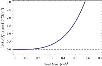
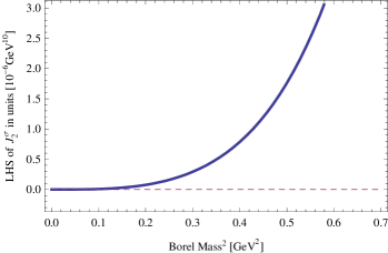
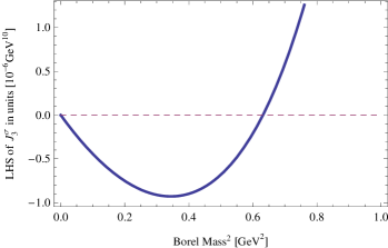
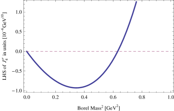
Figure 1: LHS of four interpolating currents of $\sigma$ meson, as a functions of Borel mass squared, with $s_{0}$=infinity, in units of $\rm GeV^{10}$.

To find the current with the best convergence, we have to refer to their Borel transformed correlators in numerical expressions, which are:

$$\Pi^{\sigma(\rm all)}_{1} = 1.9\times 10^{-5}M_{B}^{10}-1.9\times 10^{-8}M_{B}^{8}+9.5\times 10^{-6}M_{B}^{6}+3.7\times 10^{-8}M_{B}^{4}-8.5\times 10^{-8}M_{B}^{2},$$

$$\Pi^{\sigma(\rm all)}_{2} = 1.9\times 10^{-5}M_{B}^{10}-2.0\times 10^{-8}M_{B}^{8}+9.5\times 10^{-6}M_{B}^{6}-4.2\times 10^{-8}M_{B}^{4}-2.1\times 10^{-8}M_{B}^{2},$$

$$\Pi^{\sigma(\rm all)}_{3} = 3.2\times 10^{-6}M_{B}^{10}-2.5\times 10^{-9}M_{B}^{8}+1.6\times 10^{-6}M_{B}^{6}-6.2\times 10^{-6}M_{B}^{4}-5.1\times 10^{-6}M_{B}^{2},$$

$$\Pi^{\sigma(\rm all)}_{4} = 3.2\times 10^{-6}M_{B}^{10}-2.5\times 10^{-9}M_{B}^{8}+1.6\times 10^{-6}M_{B}^{6}+6.2\times 10^{-6}M_{B}^{4}-5.1\times 10^{-6}M_{B}^{2}.$$ (64)

From these expressions, it is obvious that current $J_{2}^{\sigma}$ shows the best convergence behavior, so we will utilize current $J_{2}^{\sigma}$ to compute the physical mass of $\sigma$. We first choose an infinite threshold to estimate the mass as the traditional sum rule has done reinders . In Figure 2, we exhibit the behavior of the mass of $\sigma$ meson as the function of $M_{B}$ for infinite and finite $s_{0}$. In traditional sum rule, if the mass as a function of $M_{B}$, has a wide minimum, then the minimum value of mass function can be perceived as the real mass of the state. From Figure 2, we observed that $M_{\sigma}$ as a function of $M_{B}^{2}$ indeed has a minimum with $M_{\sigma(\rm min)}=0.59{\rm\leavevmode\nobreak\ GeV}$ at $M_{B}^{2}=0.079{\rm\leavevmode\nobreak\ GeV}^{2}$. At this value of Borel mass, the correlation function $\Pi^{\sigma(\rm all)}_{2}=3\times 10^{-9}\leavevmode\nobreak\ {\rm GeV}^{10}$, so the positivity of LHS is kept. Although $M_{\sigma(\rm min)}$ is very close to the experimental center value $\langle M_{\sigma}\rangle\sim 0.6\rm\leavevmode\nobreak\ GeV$, the minimum is not wide enough as required. Therefore, to obtain an acceptable result, we have to adopt finite thresholds scheme zhu1 ; zhu2 ; zhu3 ; zhu4 to repeat the process of computing mass. The results for some values of threshold are presented in the right part of Figure 2. We notice that when the mass becomes weakly dependent on $M_{B}$, the value of mass is around 0.6 GeV. But we also find that as the threshold increases, the mass will increase too. This may be due to the fact that $\sigma$ is a broad resonance state. So there must be some criteria to help us dictate which value of mass is the most believable one. Combining the points of view adopted byzhu2 ; Kojo ; Matheus on judging when an acceptable sum rule is arrived, we postulate the following criteria.

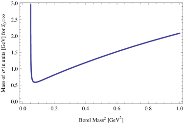
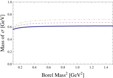
Figure 2: Mass of $\sigma$ is illustrated as function of Borel Mass squared. The left figure is in the case of infinite threshold, while the right one is in cases of finite thresholds. The results corresponding to $s_{0}$ =0.5, 0.6, 0.7 $\rm GeV^{2}$ are represented by a solid line, a dashed line and a dot-dashed line respectively.

1. The Borel transformed correlation function $\Pi(M_{B}^{2})$ should show a good positivity for almost all values of Borel mass. This is usually related the convergence of LHS.

2. The physical mass should depend weakly on the value of Borel mass in a wide region. In other words, there should be a Borel window.

3. OPE convergence. This is a strong constraint to the lower bound of the $M_{B}^{2}$ region. OPE series converge better for higher values of $M_{B}^{2}$, so that requiring a good convergence sets a lower limit to $M_{B}^{2}$. To current $J^{\sigma}_{2}$, we find such a lower limit of $M_{B}^{2}$ in the following. We first rewrite the spectral function corresponding to $J^{\sigma}_{2}$ as,

$$\rho_{\sigma}^{(\rm{OPE})}=\Sigma_{n=0}^{4}c^{(8-2n)}s^{n}=\Sigma_{n=0}^{4}\rho^{n},$$ (65)

where $c^{(8-2n)}$ denotes the operators of mass dimension $(8-2n)$, $\rho^{n}\equiv c^{(8-2n)}s^{n}$. From Eqs. (55)-(62), we learn that terms $\rho^{(3,4)}$ are perturbative contributions denoted as $\rho^{(pert)}$, in other words, they do not contain condensate. Remaining terms represent contributions from operators of dimension 4, 6 and 8. These terms are dominated by condensates including the non-perturbative effect, denoted by $\rho^{(2)}$, $\rho^{(1)}$, $\rho^{(0)}$ respectively. In Fig. 3, we present the relative contribution of $\rho^{(2)}$, $\rho^{(1)}$, $\rho^{(0)}$ to the total spectral function $\rho^{({\rm OPE})}_{\sigma}$.

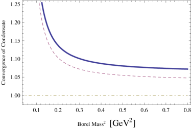
Figure 3: convergence of OPE series of spectral function related to current$J^{\sigma}_{2}$ for $s_{0}=0.6\rm{GeV}^{2}$.

The thick line denotes [$\int^{0.6}_{0}(\rho^{(pert)}+\rho^{(2)})e^{-s/M_{B}^{2}}ds/\int^{0.6}_{0}\rho^{(\rm OPE)}e^{-s/M_{B}^{2}}ds$], the dashed line signifies [$\int^{0.6}_{0}(\rho^{(pert)}+\rho^{(2)}+\rho^{(1)})e^{-s/M_{B}^{2}}ds/\int^{0.6}_{0}\rho^{(\rm OPE)}e^{-s/M_{B}^{2}}ds$], the dashed doted line represents [$\int^{0.6}_{0}(\rho^{(pert)}+\rho^{(2)}+\rho^{(1)}+\rho^{(0)})e^{-s/M_{B}^{2}}ds/\int^{0.6}_{0}\rho^{(\rm OPE)}e^{-s/M_{B}^{2}}ds$=1]. We see that, for $M_{B}^{2}>0.2\rm{GeV}^{2}$, the addition of a subsequent term in expansion (65), brings the curve closer to an asymptotic value (which is normalized to 1). Furthermore, the changes in this curve become smaller with increasing dimension. Thus, for $s_{0}=0.6\rm{GeV}^{2}$, the convergence is satisfied by $M_{B}^{2}>0.2\rm{GeV}^{2}$. For $s_{0}=0.5,\leavevmode\nobreak\ 0.7,\leavevmode\nobreak\ 0.8\rm{GeV}^{2}$, convergence limits $M_{B}^{2}>0.2,\leavevmode\nobreak\ 0.3,\leavevmode\nobreak\ 0.4\rm{GeV}^{2}$, respectively.

4. For a given threshold, the pole contribution should be sufficient large. By choosing suitable Borel mass, this can be satisfied. Since the Borel transformation suppresses the contributions from $s_{0}>M_{B}^{2}$, small value of $M_{B}^{2}$ are preferred to suppress the continuum contributions. But $M_{B}^{2}$ cannot be arbitrarily small, or it will spoil previous three requirements. To $\sigma$, we have found such optimal values of $M_{B}^{2}$ for different thresholds. We list the corresponding pole contributions in Table I. The pole contribution is defined as

$$\mbox{Pole contribution}\equiv\frac{\int^{s_{0}}_{0}e^{-s/M_{B}^{2}}\rho(s)ds}{\int^{\infty}_{0}e^{-s/M_{B}^{2}}\rho(s)ds}\,.$$ (66)

Table 1: Pole contributions of various threshold.

$s_{0}\leavevmode\nobreak\ ({\rm GeV}^{2})$	0.5	0.6	0.7	0.8
$M_{B}^{2}\leavevmode\nobreak\ ({\rm GeV}^{2})$	0.2	0.2	0.3	0.4
Pole (%)	40	52	35	25
$M_{\sigma}$ (GeV)	0.6	0.6	0.7	0.75

From this table, we can extract following information that when threshold changes from $0.5\leavevmode\nobreak\ {\rm GeV}^{2}$ to $0.8\leavevmode\nobreak\ {\rm GeV}^{2}$, the pole contribution will vary from 40% to 25% correspondingly, but reaches its maximum 52% at $M_{B}^{2}$=0.2 ${\rm GeV}^{2}$, when $s_{0}=0.6{\rm GeV}^{2}$. That the pole contribution reaches 52% implies that a good sum rule has been obtained. We get

$$m_{\sigma}=(600\pm 75)\rm{MeV},\leavevmode\nobreak\ \leavevmode\nobreak\ \leavevmode\nobreak\ \leavevmode\nobreak\ \leavevmode\nobreak\ \leavevmode\nobreak\ \leavevmode\nobreak\ \rm{with\leavevmode\nobreak\ Pole\leavevmode\nobreak\ contribution}(52\%),$$ (67)

where $(\pm 75)$ MeV originates from the error of condensates (see Eq. III.3). It is remarkable that the Pole contribution is larger than that given in zhu2 , where the Pole contribution is below 30%.

Applying the same analysis to meson $\kappa$, the LHS of four possible interpolating currents of $\kappa$ can be found in Figure 4, with threshold value $s_{0}$ being infinity.

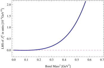
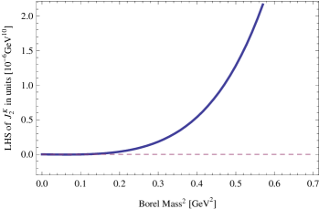
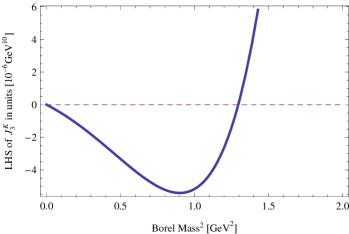
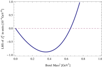
Figure 4: LHS of $\kappa$ meson as functions of Borel mass squared with $s_{0}$=infinity in units of $\rm GeV^{10}$.

The corresponding numerical expressions are listed below:

$$\Pi^{\kappa(\rm all)}_{1} = 1.9\times 10^{-5}M_{B}^{10}-1.2\times 10^{-6}M_{B}^{8}+6.7\times 10^{-6}M_{B}^{6}-1.3\times 10^{-7}M_{B}^{4}-1.2\times 10^{-7}M_{B}^{2},$$

$$\Pi^{\kappa(\rm all)}_{2} = 1.9\times 10^{-5}M_{B}^{10}-1.2\times 10^{-6}M_{B}^{8}+6.7\times 10^{-6}M_{B}^{6}-1.9\times 10^{-7}M_{B}^{4}-5.7\times 10^{-8}M_{B}^{2},$$

$$\Pi^{\kappa(\rm all)}_{3} = 3.2\times 10^{-6}M_{B}^{10}-1.9\times 10^{-7}M_{B}^{8}+1.7\times 10^{-6}M_{B}^{6}-5.2\times 10^{-6}M_{B}^{4}-4.6\times 10^{-6}M_{B}^{2},$$

$$\Pi^{\kappa(\rm all)}_{4} = 3.2\times 10^{-6}M_{B}^{10}-1.9\times 10^{-7}M_{B}^{8}+1.7\times 10^{-6}M_{B}^{6}+5.2\times 10^{-6}M_{B}^{4}-4.6\times 10^{-6}M_{B}^{2}.$$ (68)

From Figure 4 and above expressions, we notice that current $J_{2}^{\kappa}$, which is a proper mixture between tensor and pseudoscalar contents, is the best interpolating current. By setting the threshold to be infinity, we obtain an estimation for the mass of $\kappa$. As shown in Figure 5, $M_{\kappa}$ as a function of $M_{B}$ has a minimum with $M_{\kappa(\rm min)}=0.90{\rm\leavevmode\nobreak\ GeV}$ at $M_{B}^{2}=0.2{\rm\leavevmode\nobreak\ GeV}^{2}$. At this value of Borel mass, the correlation function $\Pi^{\kappa(\rm all)}_{2}=1.6\times 10^{-7}\leavevmode\nobreak\ {\rm GeV}^{10}$ , the positivity of LHS is also retained. But the minimum is still not wide enough, then the finite threshold analysis should be performed. The results are shown in the right part of Figure 5. At the Borel window, the mass of $\kappa$ is close to 0.8 GeV.

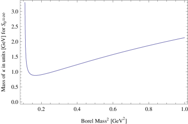
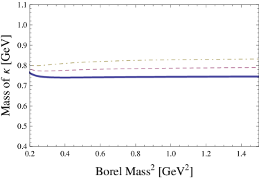
Figure 5: Mass of $\kappa$ is illustrated as function of Borel Mass squared. The left figure is in the case of infinite threshold, while the right one is in cases of finite thresholds. The results corresponding to $s_{0}$ =0.7, 0.8, 0.9 $\rm GeV^{2}$ are represented by a solid line, a dashed line and a dot-dashed line respectively.

To find the best sum rule, following the previous criteria, we find that to $\kappa$, the convergence limits $M_{B}^{2}>0.25\rm{GeV}^{2}$ for $s_{0}=0.8,\leavevmode\nobreak\ 0.9\rm{GeV}^{2}$ and $M_{B}^{2}>0.225,\leavevmode\nobreak\ 0.3\rm{GeV}^{2}$ for $s_{0}=0.7,\leavevmode\nobreak\ 1.2\rm{GeV}^{2}$, respectively. For instance, to $s_{0}=0.9\rm{GeV}^{2}$, the convergence of OPE series is shown in Fig. 6.

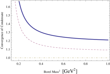
Figure 6: convergence of OPE series of spectral function related to current$J^{\kappa}_{2}$ for $s_{0}=0.9\rm{GeV}^{2}$.

The pole contributions for several values of threshold are listed in Table II.

Table 2: Pole contributions of various threshold.

$s_{0}\leavevmode\nobreak\ ({\rm GeV}^{2})$	0.7	0.8	0.9	1.2
$M_{B}^{2}\leavevmode\nobreak\ ({\rm GeV}^{2})$	0.225	0.25	0.25	0.5
Pole (%)	43	47	56	27
$M_{\kappa}$ (GeV)	0.75	0.8	0.82	0.95

When $s_{0}=0.9{\rm GeV}^{2}$, $M_{B}^{2}=0.25{\rm GeV}^{2}$, we get a pole contribution 56%. Such a large pole contribution suggests that a good sum rule has been obtained. We get the mass of $\kappa$,

$$m_{\kappa}=(820\pm 80)\rm{MeV},\leavevmode\nobreak\ \leavevmode\nobreak\ \leavevmode\nobreak\ \leavevmode\nobreak\ \leavevmode\nobreak\ \leavevmode\nobreak\ \leavevmode\nobreak\ with\leavevmode\nobreak\ Pole\leavevmode\nobreak\ contribution(56\%).$$ (69)

This pole contribution is also larger than that given by zhu2 , where the pole contribution approaches 45%.

Lastly, for $a_{+}$ and $f_{0}$ that are degenerate in OPE calculations, the LHS of four possible interpolating currents are shown in Fig. 7, with threshold value $s_{0}$ being infinity.

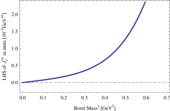
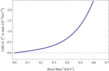
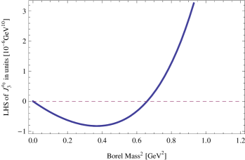
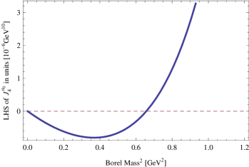
Figure 7: LHS of four interpolating currents of $a_{+}$ and $f_{0}$ as functions of Borel mass squared with $s_{0}$=infinity in units of $\rm GeV^{10}$.

Their numerical expressions are the following ones:

$$\Pi^{a+,f0(\rm all)}_{1} = 1.9\times 10^{-5}M_{B}^{10}-2.3\times 10^{-6}M_{B}^{8}+4.0\times 10^{-6}M_{B}^{6}-5.8\times 10^{-8}M_{B}^{4}+7.2\times 10^{-7}M_{B}^{2},$$

$$\Pi^{a+,f0(\rm all)}_{2} = 1.9\times 10^{-5}M_{B}^{10}-2.3\times 10^{-6}M_{B}^{8}+4.0\times 10^{-6}M_{B}^{6}-1.1\times 10^{-8}M_{B}^{4}+7.7\times 10^{-7}M_{B}^{2},$$

$$\Pi^{a+,f0(\rm all)}_{3} = 3.2\times 10^{-6}M_{B}^{10}-3.7\times 10^{-7}M_{B}^{8}+1.8\times 10^{-6}M_{B}^{6}+4.2\times 10^{-6}M_{B}^{4}-4.1\times 10^{-6}M_{B}^{2},$$

$$\Pi^{a+,f0(\rm all)}_{4} = 3.2\times 10^{-6}M_{B}^{10}-3.7\times 10^{-7}M_{B}^{8}+1.8\times 10^{-6}M_{B}^{6}+4.2\times 10^{-6}M_{B}^{4}-4.0\times 10^{-6}M_{B}^{2}.$$ (70)

From Fig. 7 and above expressions, current $J_{2}^{a_{+}}$ seems to be the best one. But when applying the traditional sum rule method to estimate mass, it turns out that there is no minimum as shown in Fig. 8. Furthermore, if we choose certain threshold and Borel mass to reproduce the experimental center value of the masses of $a_{+}$ and $f_{0}$, the pole contribution can only be around 10%. This indicates that in contrast to the success of SR analysis of $\sigma$ and $\kappa$, the SR fails to analyze $a_{+}$ and $f_{0}$, in terms of the interpolating currents deduced from their wavefunctions as tetraquarks. The reason is as follows. Jaffe’s wavefunctions are the eigenfunctions of $H_{eff}$ in Eq. (1). However, $H_{eff}$ is only an approximate description of color-magnetic interactions $H_{CM}=-\sum_{i\;j}C_{ij}(\lambda_{i}\cdot\lambda_{j})(\overrightarrow{\sigma}_{i}\cdot\overrightarrow{\sigma}_{j})$ DGG ; hogaasen1 ; hogaasen2 ; dy . If the flavor $SU(3)_{f}$-symmetry is exact, the interaction strengthes $C_{ij}$ are flavor-$(ij)$ independent, i.e., $C_{ij}=C$, then $H_{CM}=H_{eff}$. But for real QCD, the constituent mass $m^{c}_{u}\approx m^{c}_{d}$, while $m^{c}_{s}>\hat{m^{c}}\equiv(m^{c}_{u}+m^{c}_{d})/2$. So $SU(3)_{f}$ must be broken within order $\mathcal{O}((m^{c}_{s}-\hat{m^{c}})/m^{c}_{s})\sim\mathcal{O}(0.3)$. Therefore, both $H_{eff}$ and Jaffe’s wavefunction $|0^{+},\underline{9}\rangle$ will suffer of this $SU(3)_{f}$ breaking effect. In other words, $|0^{+},\underline{9}\rangle$ can only be thought of as the leading term of the eigenfunction of $H_{CM}$, without considering the correction from the next leading term caused by the strange quark content in $0^{+}$-tetraquarks. In $\sigma(\{ud\}\{\bar{u}\bar{d}\})$, there is no strange quark, so no such kind of corrections, hence $|\sigma\rangle=|0^{+},\underline{9}\rangle_{\sigma}$ is suitable. In $\kappa(\{ud\}\{\bar{d}\bar{s}\})$, there is one strange quark, its correction is relatively small, and the wavefunction $|0^{+},\underline{9}\rangle_{\kappa}$ may be still valid to some extent. This is supported by numerical results. However, for $f_{0}({1\over\sqrt{2}}(\{us\}\{\bar{u}\bar{s}\}+\{ds\}\{\bar{d}\bar{s}\}))$ or $a_{+}(\{us\}\{\bar{d}\bar{s}\})$, there are two strange quarks, the $SU(3)_{f}$ breaking effects is doubled. To these cases, one cannot insist the Jaffe’s wavefunctions $|f_{0}\rangle=|0^{+},\underline{9}\rangle_{f_{0}}$ and $|a_{+}\rangle=|0^{+},\underline{9}\rangle_{a_{+}}$ be still good enough to describe the non-perturbative QCD physics. Above all, we speculate that a legitimate SR analysis for $f_{0}$ and $a_{+}$ should be based on the tetraquark’s color-magnetic wavefunctions which are more precise, encoding the $SU(3)_{f}$-symmetry breaking effects.

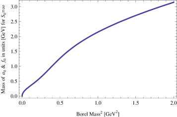
Figure 8: Mass of $a_{+}$ and $f_{0}$ as function of Borel mass $M_{B}$ with $s_{0}$ being infinity.

IV The direct instanton contribution to sum rule

IV.1 Analytic results

In addition to the contribution of power type from the OPE expansion to the QCD SR, there are exponential contributions coming from direct instanton contributions. The direct instantion contributions originate from ’t Hooft’s instanton induced interaction tHooft . If the physics considered is relevant to two flavors, instanton effects induce a four-fermion interaction, as illustrated in Fig. 9 (usually called two-body single instanton contribution defined in lee2 ). In the framework of sum rule, this kind of instanton effect can be encoded in the quark propagator. Now the quark propagator has two terms,

$$S^{q}_{ab}=S^{q({\rm st})}_{ab}+S^{q({\rm inst})}_{ab}.$$ (71)

$S^{q({\rm st})}_{ab}$ corresponds to standard quark propagator (Eqs. (53) and (54)) in Euclidean space, $S^{q({\rm inst})}_{ab}$ is related to instanton contribution and can be calculated by using the following formula in Euclidean space and regular gauge,

$$S^{q({\rm inst})}_{ab}=A_{q}(x,y)\gamma_{\mu}\gamma_{\nu}(1+\gamma_{5})(U\tau_{\mu}^{+}\tau_{\nu}^{-}U^{\dagger})_{ab},$$ (72)

where

$$A_{q}(x,y)=-i\frac{r^{2}}{16\pi^{2}m_{q}^{\ast}}\phi(x-z_{0})\phi(y-z_{0})$$ (73)

and

$$\phi(x-z_{0})=\frac{1}{[(x-z_{0})^{2}+r^{2}]^{3/2}}.$$ (74)

Here $r$ stands for the instanton size, $z_{0}$ for the center of the instanton. $U$ represents the color orientation matrix of the instanton in $SU(3)_{c}$ and $\tau^{+,-}_{\mu,\nu}$ are $SU(2)_{c}$ matrices. The effective mass of quark on the instanton vacuum is $m_{q}^{\ast}=m_{q}-2\pi^{2}r^{2}_{c}\langle\bar{q}q\rangle/3$ with current quark mass $m_{q}$, here $q\in\{u,d,s\}$. At the final stage, we multiply the result by a factor of two to take into account the anti-instanton effect and integrate over the color orientation and instanton size. When integrating over the instanton size, Shuryak’s instanton liquid model schafer for QCD vacuum with density $n_{r}=n_{eff}\delta(r-r_{c})$ has been used.

Figure 9: The leading direct instanton contribution to the correlator, where “I” represents the instanton.

With the definition $Q^{2}=-q^{2}$, the direct instanton contributions to the scalar nonet are listed below, corresponding to above two diagrams. Here, we only exhibit the contributions to $\sigma$-correlator, and the reader can find the results of other tetraquarks in appendix. We denote the total contributions from intanton and anti-instanton by “inst”. Recalling that the direct instanton contribution is possible only for different quark flavors, so in case of $\sigma$, there is no direct three-body instanton contribution (from instanton induced six-fermion interaction). But to $\kappa$, $a_{+}$, $f_{0}$, three-body instanton contribution might be important. However, in this paper, we only present the two-body instanton contributions for these mesons, to capture the main physics.

$$\Pi_{TT}^{\sigma(\rm inst)} = \frac{156n_{eff}r_{c}^{4}\langle\bar{q}q\rangle^{2}}{3\pi^{4}m_{q}^{\ast 2}}f_{0}(Q),$$ (75)

$$\Pi_{SS}^{\sigma(\rm inst)} = \frac{32n_{eff}r_{c}^{4}}{\pi^{8}m_{q}^{\ast 2}}f_{6}(Q)+\frac{19n_{eff}r_{c}^{4}\langle\bar{q}q\rangle^{2}}{18\pi^{4}m_{q}^{\ast 2}}f_{0}(Q),$$ (76)

$$\Pi_{PP}^{\sigma(\rm inst)} = -\frac{32n_{eff}r_{c}^{4}}{\pi^{8}m_{q}^{\ast 2}}f_{6}(Q)+\frac{19n_{eff}r_{c}^{4}\langle\bar{q}q\rangle^{2}}{18\pi^{4}m_{q}^{\ast 2}}f_{0}(Q),$$ (77)

$$\Pi_{TS}^{\sigma(\rm inst)} = \Pi_{ST}^{\sigma(\rm inst)}=\frac{2n_{eff}r_{c}^{4}\langle\bar{q}q\rangle^{2}}{\pi^{4}m_{q}^{\ast 2}}f_{0}(Q),$$ (78)

$$\Pi_{TP}^{\sigma(\rm inst)} = \Pi_{PT}^{\sigma(\rm inst)}=\frac{2n_{eff}r_{c}^{4}\langle\bar{q}q\rangle^{2}}{\pi^{4}m_{q}^{\ast 2}}f_{0}(Q),$$ (79)

$$\Pi_{AA}^{\sigma(\rm inst)} = \frac{48n_{eff}r_{c}^{4}}{\pi^{8}m_{q}^{\ast 2}}f_{6}(Q)+\frac{68n_{eff}r_{c}^{4}\langle\bar{q}q\rangle^{2}}{9\pi^{4}m_{q}^{\ast 2}}f_{0}(Q),$$ (80)

$$\Pi_{AS}^{\sigma(\rm inst)} = \Pi_{SA}^{\sigma(\rm inst)}=-\frac{20n_{eff}r_{c}^{4}}{\pi^{8}m_{q}^{\ast 2}}f_{6}(Q),$$ (81)

$$\Pi_{AP}^{\sigma(\rm inst)} = \Pi_{PA}^{\sigma(\rm inst)}=-\frac{20n_{eff}r_{c}^{4}}{\pi^{8}m_{q}^{\ast 2}}f_{6}(Q).$$ (82)

In above expressions,

$$f_{6}(Q) = \int d^{4}z_{0}\int d^{4}x\frac{e^{iq\cdot x}}{x^{6}[z_{0}^{2}+r_{c}^{2}]^{3}[(x-z_{0})^{2}+r_{c}^{2}]^{3}},$$

$$f_{0}(Q) = \int d^{4}z_{0}\int d^{4}x\frac{e^{iq\cdot x}}{[z_{0}^{2}+r_{c}^{2}]^{3}[(x-z_{0})^{2}+r_{c}^{2}]^{3}}.$$ (83)

The Borel transformation of $f_{6}(Q)$ and $f_{0}(Q)$ are:

$$\hat{B}[f_{6}(Q)] = -\frac{\pi^{4}M^{12}_{B}}{2^{13}}\int^{1}_{0}dt\int^{1}_{0}dy\frac{e^{-M^{2}_{B}r_{c}^{2}/(4ty(1-y))}}{y^{2}(1-y)^{2}}(X^{2}+5X^{3}+10X^{4}$$

$$+10X^{5}+5X^{6}+X^{7}),$$

$$\hat{B}[f_{0}(Q)] = \frac{\pi^{4}M^{6}_{B}}{16}e^{-M^{2}_{B}r_{c}^{2}/2}(K_{0}(M^{2}_{B}r_{c}^{2}/2)+K_{1}(M^{2}_{B}r_{c}^{2}/2)),$$ (84)

where we adopt the notations in paper lee2 , $X=(1-t)/t$ and $K_{n}(x)$ is the McDonald function.

IV.2 Numeric analysis of QCD sum rule with instanton effects

To evaluate the direct instanton effects quantitatively, we make use of the following relation between the parameters of Shuryak instanton model schafer .

$$\frac{n_{eff}}{m_{q}^{\ast 2}}=\frac{3}{4\pi^{2}r_{c}^{2}}\leavevmode\nobreak\ \leavevmode\nobreak\ \leavevmode\nobreak\ \leavevmode\nobreak\ \leavevmode\nobreak\ q\in\{u,\leavevmode\nobreak\ d\},$$ (85)

with

$$r_{c}=1.6\leavevmode\nobreak\ \mbox{GeV}^{-1}.$$ (86)

Considering the single instanton effects, the left hand sum rule becomes:

$$\Pi_{\rm LHS}(Q^{2})=\Pi^{\rm OPE}(Q^{2})+\Pi^{\rm inst}(Q^{2}).$$ (87)

After Borel transforming the both side of the QCD sum rule, we obtain the following relation

$$\mathcal{B}_{M_{B}^{2}}\Pi^{\rm OPE}(Q^{2})+\mathcal{B}_{M_{B}^{2}}\Pi^{\rm inst}(Q^{2})=2\pi f_{X}^{2}m_{X}^{8}e^{-m_{X}^{2}/M_{B}^{2}}.$$ (88)

In above expressions,

$$\mathcal{B}_{M_{B}^{2}}\Pi^{{\rm OPE}}(Q^{2})=\int^{S_{0}}_{0}e^{-s/M_{B}^{2}}\rho^{\rm OPE}(s)ds,$$ (89)

where we have chosen a finite threshold to suppress the contribution from continuum. Utilizing the results in previous sections, the left hand sum rule can be performed for each possible interpolating current in (43) belonging to a certain meson. Then we can make use of the best current to fit the right hand sum rule to obtain the mass and residue. This approach was first suggested by lee2 . In the following, for the sake of simplicity, we will only present a detailed analysis for $\sigma$ meson. For other mesons, the results are also exhibited.

In Fig. 10, we show the Borel transformed correlators $\Pi(M_{B}^{2})$, including the instanton effects, at threshold value $s_{0}$=0.6 $\mbox{GeV}^{2}$. From the Figure, we see that the instanton contributions are not always positive. To current $J_{1}^{\sigma}$, they provide little negative contributions, and spoil the positivity of LHS obviously, when Borel mass is small; to current $J_{3}^{\sigma}$ and $J_{4}^{\sigma}$, instanton effects make the LHS rather negative, and this may be the usually called dangerous instanton contribution to sum rule lee2 ; only to current $J_{2}^{\sigma}$, the instanton effects improve the OPE calculation completely. This feature can be seen more clearly, if we notice that in Eqs. (75)-(79):

$$\Pi_{TT}^{\sigma(\rm inst)} = \frac{156n_{eff}r_{c}^{4}\langle\bar{q}q\rangle^{2}}{3\pi^{4}m_{q}^{\ast 2}}f_{0}(Q),$$

$$\Pi_{PP}^{\sigma(\rm inst)} = -\frac{32n_{eff}r_{c}^{4}}{\pi^{8}m_{q}^{\ast 2}}f_{6}(Q)+\frac{19n_{eff}r_{c}^{4}\langle\bar{q}q\rangle^{2}}{18\pi^{4}m_{q}^{\ast 2}}f_{0}(Q),$$

$$\Pi_{TP}^{\sigma(\rm inst)} = \Pi_{PT}^{\sigma(\rm inst)}=\frac{2n_{eff}r_{c}^{4}\langle\bar{q}q\rangle^{2}}{\pi^{4}m_{q}^{\ast 2}}f_{0}(Q).$$ (90)

In above expressions, the coefficients of $f_{0}(Q)$ are positive, while the coefficient of $f_{6}(Q)$ is negative. After Borel transformation, $f_{0}(Q)$ and $f_{6}(Q)$ are just as in Eq. (IV.1). Numerically, $\hat{B}[f_{0}(Q)]$ is always positive, but $\hat{B}[f_{6}(Q)]$ is always negative, so totally, the instanton contributions to the current $J_{2}^{\sigma}$ are positive. From Fig. 10, it is clear that the instanton contributions improve the convergence of current $J_{2}^{\sigma}$ when Borel mass is small.

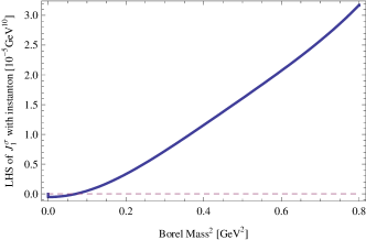
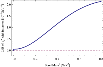
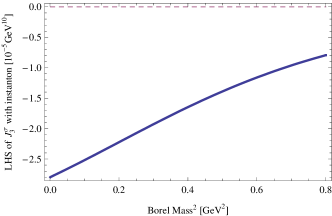
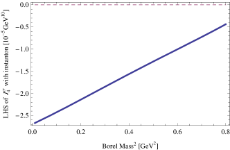
Figure 10: LHS of $\sigma$ including the instanton effects of four interpolating currents with $s_{0}$=0.6 $\mbox{GeV}^{2}$.

At this moment, we can use the numeric results associated with LHS of current $J_{2}^{\sigma}$, at threshold value 0.6 $\mbox{GeV}^{2}$, to fit the RHS in single resonance approximation that is just the Eq. (88), as illustrated in Fig. 11. That choosing 0.6 $\mbox{GeV}^{2}$ as the value of threshold is inspired by previous OPE results. The fitted mass and residues are listed in Table 3:

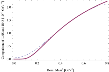
Figure 11: The dashed and thick lines represent the left hand sum rule and right hand sum rule, respectively. To RHS, the mass and residue are presented in Table III.

From the table, we notice that after adding the instanton contribution, the mass of $\sigma$ meson is still close to OPE result Eq.(67). Then the instanton contribution is compatible with OPE results. It suggests that the physical mass of $\sigma$ depends weakly on the choice of QCD vacuum.

Table 3: Fitted masses and residues in single resonance approximation

$s_{0}({\rm GeV}^{2})$	$M_{\sigma}$(GeV)	${f}_{\sigma}(10^{-2}\rm GeV)$
0.6	0.72	0.94
1	0.73	0.93

In the case of $s_{0}=0.6\rm{GeV^{2}}$, considering a $(\pm 10\%)$ variation of instanton size $r_{c}=1.6\pm 0.2$, we find a corresponding variation of $m_{\sigma}=720^{-100}_{+\leavevmode\nobreak\ 60}\rm{MeV}$ and $f_{\sigma}=0.94^{+\leavevmode\nobreak\ 0.4}_{-0.07}(10^{-2}\rm GeV)$. It seems like that the change of physical quantity lies within an acceptable range and the residue is more sensitive to the variation of instanton size compared with the mass. In Kojo , the authors discussed the meaning of the residue. In their notations, residue is defined as $\lambda^{2}=2\pi f_{X}^{2}M_{X}^{8}$. So we obtain a residue $\lambda^{2}=4\times 10^{-5}{\rm GeV^{10}}$, which is larger than $\lambda^{2}=2\times 10^{-6}{\rm GeV^{10}}$ presented in Kojo . According to the explanation of Kojo , large residue signifies the interpolating current operators have enough overlaps to the resonance states and the sum rule constructed with approximate OPE may contain enough information for the resonance to be extracted. So in our case, evaluating OPE up to dimension eight condensates seems reasonable.

Finally, in order to investigate further the widths of the $\sigma$ meson states, it is necessary to find out three point correlation functions for $\sigma\rightarrow\pi\pi$, which has got out of the scope of this paper.

As for other mesons, the current $J_{2}$ still shows the best performance. The fitted masses and residues for $\kappa$, $a_{+}$ and $f_{0}$ are presented in Table IV, V and VI in appendix , respectively.

V Conclusion and Discussion

In this paper, we study the $0^{+}$ nonet mesons as tetraquark states with interpolating currents induced from the color-magnetic wavefunction. This wavefunction is the eigenfunction of the effective color-magnetic Hamiltonian with the lowest eigenvalue, meaning that the state with this wavefunction is the most stable one and is most probable to be observed in experiments. Our approach can be recognized as constructing interpolating currents dynamically. We find that based on a current which is a proper mixture of the tensor and pseudoscalar contents, a good sum rule can be obtained. Our result can be perceived as a direct support to multiquark scenario described by the color-magnetic interaction, by means of QCD sum rule.

In the SR calculations performed in this paper, we have taken into account the contributions from operators up to dimension $d=8$ in the OPE. The results of SR analysis without instanton effects for $0^{+}$ meson nonet $\{\sigma,\;\kappa,\;f_{0},\;a_{+}\}$ are :

1. $\sigma$: In the SR analysis , a good Borel stability turns out in the region $M_{B}^{2}>0.2\leavevmode\nobreak\ {\rm GeV}^{2}$. Taking $M_{B}^{2}\approx 0.2\leavevmode\nobreak\ {\rm GeV}^{2}$ and the threshold $s_{0}\approx 0.6\leavevmode\nobreak\ {\rm GeV}^{2}$, the largest pole contribution is $52\%$ implying that a good SR analysis is achieved. Where we extract the mass of $\sigma$ $(600\pm 75)$ MeV.

2. $\kappa$: A good sum rule was found when $s_{0}=0.9\rm{GeV}^{2}$, $M^{2}_{B}>0.25\rm{GeV}^{2}$. We obtain $\kappa$ mass $(820\pm 80)$MeV with pole contribution approaching 56%.

3. $f_{0}\leavevmode\nobreak\ {\rm and}\leavevmode\nobreak\ a_{+}$: to obtain a mass about 1 GeV by choosing the threshold and Borel mass, the pole contributions in SR are always around 10%. This indicates that the SR fails to analyze $a_{+}$ and $f_{0}$ by using the interpolating currents deduced from the wavefunctions. We guess the reason is that in $f_{0}({1\over\sqrt{2}}(\{us\}\{\bar{u}\bar{s}\}+\{ds\}\{\bar{d}\bar{s}\}))$ or $a_{+}(\{us\}\{\bar{d}\bar{s}\})$, there are two strange quarks, so $SU(3)_{f}$ breaking effects are too strong to be negligible. This causes the Jaffe’s wavefunctions $|f_{0}\rangle=|0^{+},\underline{9}\rangle_{f_{0}}$ and $|a_{+}\rangle=|0^{+},\underline{9}\rangle_{a_{+}}$ to miss some aspects of the $f_{0}$- and $a_{+}$-physics. We speculate that a legitimate SR analysis for them should be based on the tetraquark color-magnetic wavefunctions including the $SU(3)_{f}$-breaking effects due to $m_{s}^{c}>\hat{m}^{c}$.

Proceed stepwise, we consider the direct instanton contribution. To the current $J_{2}$, the instanton effects are completely positive. Numerically, this positive effects improve the small Borel mass behavior of the Borel transformed correlator of current $J_{2}$. Meanwhile, adding instanton effects, the LHS gives a result compatible with OPE results.

Finally, we go one step further and believe that the idea demonstrated in this paper also applies to $0^{-}$-$q^{3}\bar{q}^{3}$ system. In DPY , the authors have successfully extended Jaffe’s method from $q^{2}\bar{q}^{2}$ to $q^{3}\bar{q}^{3}$ six-quark system (i.e., baryonium). One of the non-trivial results in DPY for baryonium is the existance of a counterpart of $\sigma$. We denote this state by $|0^{-},\underline{1}_{f}\rangle$. Corresponding to Eq. (3) for tetraquark, DPY shows

$$H_{eff}|0^{-},\underline{1}_{f}\rangle=-82.533\widetilde{C}|0^{-},\underline{1}_{f}\rangle.$$ (91)

In baryonium contents, its color-spin-flavor wavefunction can be expressed as:

$$|0^{-},\underline{1}_{f}\rangle \equiv |\mathbf{1},\mathbf{}1_{f}\otimes\mathbf{1}_{f}\rangle_{1}=0.591|(\mathbf{56}_{cs},\mathbf{10}_{c},\mathbf{4};\mathbf{1}_{f}),(\overline{\mathbf{56}}_{cs},\overline{\mathbf{10}}_{c},\mathbf{4};\mathbf{1}_{f}),\mathbf{1}_{c},\mathbf{1};\mathbf{1}_{f}\otimes\mathbf{1}_{f}\rangle$$ (92)

$$+0.807|(\mathbf{56}_{cs},\mathbf{8}_{c},\mathbf{2};\mathbf{1}_{f}),(\overline{\mathbf{56}}_{cs},\mathbf{8}_{c},\mathbf{2};\mathbf{1}_{f}),\mathbf{1}_{c},\mathbf{1};\mathbf{1}_{f}\otimes\mathbf{1}_{f}\rangle,$$

where the notations in DPY have been used. Like $|\sigma\rangle$, $|0^{-},\underline{1}_{f}\rangle$ has the largest mass defect among all the baryoniums. This implies that $|0^{-},\underline{1}_{f}\rangle$, the lightest baryonium meson, may represent a stable physical state. Like Eq. (8), the mass of $|0^{-},\underline{1}_{f}\rangle$ can be estimated roughly in the naive constituent quark model as follows

$$m_{|0^{-},\underline{1}_{f}\rangle} \approx \langle\sum_{i}m_{i}^{c}-\widetilde{C}\sum_{i\;j}(\lambda_{i}\cdot\lambda_{j})(\overrightarrow{\sigma}_{i}\cdot\overrightarrow{\sigma}_{j})\rangle_{|0^{-},\underline{1}_{f}\rangle}$$ (93)

$$\approx (4\times 360{\rm MeV}+2\times 540{\rm MeV})-82.533\times\left({4\times 20{\rm MeV}+2\times 15{\rm MeV}\over 6}\right)$$

$$\approx 1.007{\rm GeV}.$$

We find that the mass of $|0^{-},\underline{1}_{f}\rangle$ is close to that of $\eta^{\prime}(960)$ Yao:2006px . Furthermore, their quantum numbers are the same. So in the multiquark picture, we might identify $|0^{-},\underline{1}_{f}\rangle$ as $\eta^{\prime}(960)$, or perceive $\eta^{\prime}(960)$ as a baryonium or a Fermi-Yang meson FY . Alternatively, there may be a large weight baryonium component in $\eta^{\prime}(960)$. Usually, in the $q\bar{q}$-picture, the mass of $\eta^{\prime}$ is attributed to $U(1)_{A}$ anomaly with non-trivial $\theta$ vacuum in QCD tHooft . However, that scenario has not excluded other schemes yet (e.g., see donoghue ). In our case, a further examination to the conjecture on $\eta^{\prime}$ in non-perturbative QCD should be meaningful. Since we have already known the color-magnetic wavefunction for $|0^{-},\underline{1}_{f}\rangle$, following the method presented in this paper, a SR analysis is straightforward. The result will be helpful to understand two interesting experimental measurements that may reveal the baryonium content of $\eta^{\prime}$. Those experiments are that:

i) to measure the anomalous enhancement near the mass threshold in the $p\bar{p}$ invariant-mass spectrum from $J/\psi\rightarrow\gamma p\bar{p}$ reported by BES BES1 .

ii) to observe resonance $X(1835)$ in $J/\psi\rightarrow\gamma\pi^{+}\pi^{-}\eta^{\prime}$ BES2 . In BES1 the data fitting indicates that the enhancement is a S-wave Breit-Wigner resonance $X(1835)$ 1 . It has been estimated that the decay branching fraction $B(X\rightarrow p\bar{p})>4\%$ 2 . The decay mode of $X\rightarrow p\bar{p}$ is due to the tail effect of enhancement resonance of $X(1835)$ near the threshold of process $J/\psi\rightarrow\gamma p\bar{p}$, therefore the fact of $B(X\rightarrow p\bar{p})>4\%$ means the coupling between $X$ and $p\bar{p}$ is very very strong. The most natural interpretation to this fact is that $X(1835)$ is simply a bound state of $p-\bar{p}$. Namely, $X(1835)$ is a $q^{3}\bar{q}^{3}$-baryonium molecular state datta ; yan . In another hand, the major decay mode for $X(1835)$ is $X(1835)\rightarrow\pi^{+}\pi^{-}\eta^{\prime}$ observed by BES BES2 . It indicates that $X(1835)$ is a molecular exciting state of meson $\eta^{\prime}$ yan . Consequently, the quark component of $\eta^{\prime}$ should be same as $X(1835)$, i.e., $\eta^{\prime}$ would be a $0^{-}$-baryonium meson, or a meson with large weight baryonium component. BES observations BES1 ; BES2 provide evidence to this multiquark picture for $\eta^{\prime}$ meson.

Appendix A

A.1 Formulas of necessary spectral functions of $\kappa$, $a_{+}$ and $f_{0}$

For $\kappa$ $(\{ud\}\{\bar{s}\bar{d}\})$, since the current mass $m_{s}$ is much bigger than $m_{u},m_{d}$, we can ignore terms proportional to $m_{u},m_{d}$ when listing the necessary spectral functions. Having done this, the length of formulas will be shortened, and the reader can have a clear impression about the structure of spectral functions. We will do the same thing for $a_{+}$ and $f_{0}$. However, in numerical calculations, the contributions from the $u,d$ quark mass terms have been taken into account. The spectral functions are the followings:

$$\rho^{\kappa\rm OPE}_{T,T} = \frac{s^{4}}{1280\pi^{6}}-\frac{m_{s}^{2}}{64\pi^{6}}s^{3}+(\frac{11\langle\textsl{g}^{2}GG\rangle}{768\pi^{6}}+\frac{m_{s}\langle\bar{s}s\rangle}{8\pi^{4}})s^{2}-\frac{11m_{s}^{2}\langle\textsl{g}^{2}GG\rangle}{256\pi^{6}}s+\frac{11m_{s}\langle\textsl{g}^{2}GG\rangle\langle\bar{s}s\rangle}{192\pi^{4}},$$ (94)

$$\rho^{\kappa\rm OPE}_{S,S} = \frac{s^{4}}{61440\pi^{6}}-\frac{{m_{s}}^{2}s^{3}}{3072\pi^{6}}+(\frac{\langle\textsl{g}^{2}GG\rangle}{6144\pi^{6}}-\frac{{m_{s}}\langle\bar{q}q\rangle}{192\pi^{4}}+\frac{{m_{s}}\langle\bar{s}s\rangle}{384\pi^{4}})s^{2}$$ (95)

$$+(-\frac{m_{s}^{2}\langle\textsl{g}^{2}GG\rangle}{2048\pi^{6}}-\frac{m_{s}\langle\textsl{g}\bar{q}\sigma Gq\rangle}{128\pi^{4}}+\frac{\langle\bar{q}q\rangle^{2}}{24\pi^{2}}+\frac{\langle\bar{q}q\rangle\langle\bar{s}s\rangle}{24\pi^{2}})s$$

$$-\frac{m_{s}^{2}\langle\bar{q}q\rangle^{2}}{12\pi^{2}}-\frac{m_{s}\langle\textsl{g}^{2}GG\rangle\langle\bar{q}q\rangle}{768\pi^{4}}+\frac{m_{s}\langle\textsl{g}^{2}GG\rangle\langle\bar{s}s\rangle}{1536\pi^{4}}+\frac{\langle\bar{q}q\rangle\langle\textsl{g}\bar{q}\sigma Gq\rangle}{24\pi^{2}}+\frac{\langle\bar{s}s\rangle\langle\textsl{g}\bar{q}\sigma Gq\rangle}{48\pi^{2}}+\frac{\langle\bar{q}q\rangle\langle\textsl{g}\bar{q}\sigma Gq\rangle}{48\pi^{2}},$$

$$\rho^{\kappa\rm OPE}_{T,S} = \rho^{\kappa\rm OPE}_{S,T}=-\frac{\langle\textsl{g}^{2}GG\rangle}{1024\pi^{6}}s^{2}+\frac{3\langle\textsl{g}^{2}GG\rangle m_{s}^{2}}{1024\pi^{6}}s-\frac{\langle\textsl{g}^{2}GG\rangle\langle\bar{s}s\rangle m_{s}}{256\pi^{4}},$$ (96)

$$\rho^{\kappa\rm OPE}_{P,P} = \frac{s^{4}}{61440\pi^{6}}-\frac{m_{s}^{2}}{3072\pi^{6}}s^{3}+(\frac{\langle\bar{q}q\rangle m_{s}}{192\pi^{4}}+\frac{\langle\bar{s}s\rangle m_{s}}{384\pi^{4}}+\frac{\langle\textsl{g}^{2}GG\rangle}{6144\pi^{6}})s^{2}-(\frac{\langle\bar{q}q\rangle^{2}}{24\pi^{2}}+\frac{\langle\bar{q}q\rangle\langle\bar{s}s\rangle}{24\pi^{2}}-\frac{\langle\textsl{g}\bar{q}\sigma Gq\rangle m_{s}}{128\pi^{4}}$$ (97)

$$+\frac{\langle\textsl{g}^{2}GG\rangle m_{s}^{2}}{2048\pi^{6}})s+(\frac{m_{s}^{2}\langle\bar{q}q\rangle^{2}}{12\pi^{2}}-\frac{\langle\textsl{g}\bar{s}\sigma Gs\rangle\langle\bar{q}q\rangle}{48\pi^{2}}-\frac{\langle\textsl{g}\bar{q}\sigma Gq\rangle(\langle\bar{s}s\rangle+2\langle\bar{q}q\rangle)}{48\pi^{2}}+\frac{\langle\textsl{g}^{2}GG\rangle(\langle\bar{q}q\rangle+\langle\bar{s}s\rangle)m_{s}}{1536\pi^{4}}),$$

$$\rho^{\kappa\rm OPE}_{T,P} = \rho^{\kappa\rm OPE}_{P,T}=-\frac{\langle\textsl{g}^{2}GG\rangle}{1024\pi^{6}}s^{2}+\frac{3\langle\textsl{g}^{2}GG\rangle m_{s}^{2}}{1024\pi^{6}}s-\frac{\langle\textsl{g}^{2}GG\rangle\langle\bar{s}s\rangle m_{s}}{256\pi^{4}},$$ (98)

$$\rho^{\kappa\rm OPE}_{A,A} = \frac{s^{4}}{7680\pi^{6}}-\frac{m_{s}^{2}}{384\pi^{6}}s^{3}+(\frac{m_{s}(\langle\bar{s}s\rangle-\langle\bar{q}q\rangle)}{48\pi^{4}}+\frac{5\langle\textsl{g}^{2}GG\rangle}{3072\pi^{6}})s^{2}-(\frac{\langle\textsl{g}\bar{q}\sigma Gq\rangle m_{s}}{32\pi^{4}}+\frac{5\langle\textsl{g}^{2}GG\rangle m_{s}^{2}}{1024\pi^{6}}-\frac{\langle\bar{q}q\rangle\langle\bar{s}s\rangle}{6\pi^{2}}$$ (99)

$$-\frac{\langle\bar{q}q\rangle\langle\bar{q}q\rangle}{6\pi^{2}})s+(\frac{\langle\textsl{g}\bar{q}\sigma Gq\rangle(2\langle\bar{q}q\rangle+\langle\bar{s}s\rangle)}{12\pi^{2}}-\frac{\langle\bar{q}q\rangle^{2}m_{s}^{2}}{3\pi^{2}}+\frac{m_{s}\langle\textsl{g}^{2}GG\rangle(5\langle\bar{s}s\rangle-2\langle\bar{q}q\rangle)}{768\pi^{4}}+\frac{\langle\textsl{g}\bar{s}\sigma Gs\rangle\langle\bar{q}q\rangle}{12\pi^{2}}),$$

$$\rho^{\kappa\rm OPE}_{A,S} = \rho^{\kappa\rm OPE}_{S,A}=\frac{\langle\textsl{g}^{2}GG\rangle m_{s}\langle\bar{q}q\rangle}{256\pi^{4}},$$ (100)

$$\rho^{\kappa\rm OPE}_{A,P} = \rho^{\kappa\rm OPE}_{P,A}=0.\leavevmode\nobreak\ \leavevmode\nobreak\ \leavevmode\nobreak\ \leavevmode\nobreak\ \leavevmode\nobreak\ \leavevmode\nobreak\ \leavevmode\nobreak\ \leavevmode\nobreak\ \leavevmode\nobreak\ \leavevmode\nobreak\ \leavevmode\nobreak\ \leavevmode\nobreak\ \leavevmode\nobreak\ \leavevmode\nobreak\ \leavevmode\nobreak\ \leavevmode\nobreak\ \leavevmode\nobreak\ \leavevmode\nobreak\ \leavevmode\nobreak\ \leavevmode\nobreak\ \leavevmode\nobreak\ \leavevmode\nobreak\ \leavevmode\nobreak\ \leavevmode\nobreak\ \leavevmode\nobreak\ \leavevmode\nobreak\ \leavevmode\nobreak\ \leavevmode\nobreak\ \leavevmode\nobreak\ \leavevmode\nobreak\ \leavevmode\nobreak\ \leavevmode\nobreak\ \leavevmode\nobreak\ \leavevmode\nobreak\ \leavevmode\nobreak\ \leavevmode\nobreak\ \leavevmode\nobreak\ \leavevmode\nobreak\ \leavevmode\nobreak\ \leavevmode\nobreak\ \leavevmode\nobreak\ \leavevmode\nobreak\ \leavevmode\nobreak\ \leavevmode\nobreak\ \leavevmode\nobreak\ \leavevmode\nobreak\ \leavevmode\nobreak\ \leavevmode\nobreak\ \leavevmode\nobreak\ \leavevmode\nobreak\ \leavevmode\nobreak\ \leavevmode\nobreak\ \leavevmode\nobreak\ \leavevmode\nobreak\ \leavevmode\nobreak\ \leavevmode\nobreak\ \leavevmode\nobreak\ \leavevmode\nobreak\ \leavevmode\nobreak\ \leavevmode\nobreak\ \leavevmode\nobreak\ \leavevmode\nobreak\ \leavevmode\nobreak\ \leavevmode\nobreak\ \leavevmode\nobreak\ \leavevmode\nobreak\ \leavevmode\nobreak\ \leavevmode\nobreak\ \leavevmode\nobreak\ \leavevmode\nobreak\ \leavevmode\nobreak\ \leavevmode\nobreak\ \leavevmode\nobreak\ \leavevmode\nobreak\ \leavevmode\nobreak\ \leavevmode\nobreak\ \leavevmode\nobreak\ \leavevmode\nobreak\ \leavevmode\nobreak\ \leavevmode\nobreak\ \leavevmode\nobreak\$$ (101)

For $a_{+}\leavevmode\nobreak\ (\{us\}\{\bar{d}\bar{s}\})$ and $f_{0}\leavevmode\nobreak\ (\frac{1}{\sqrt{2}}(\{su\}\{\bar{s}\bar{u}\}+\{sd\}\{\bar{s}\bar{d}\})$, we only list the spectral functions for $a_{+}$ below. This is because in the widely adopted scheme Eq. (53), $u$ and $d$ quark take the same value of current masses and condensates, which leads to a direct consequence that from the OPE calculation of the correlators of currents, we can not discern $a_{+}$ and $f_{0}$. In other words, to each kind interpolating current in Eq. (43), the correlators of $a_{+}$’s and the correlators of $f_{0}$’s take the same expressions after completing the OPE calculation.

$$\rho^{a_{+}\rm OPE}_{T,T} = \frac{s^{4}}{1280}-\frac{m_{s}^{2}}{32\pi^{6}}s^{3}+(\frac{3m_{s}^{4}}{16\pi^{6}}+\frac{\langle\bar{s}s\rangle m_{s}}{4\pi^{4}}+\frac{11\langle\textsl{g}^{2}GG\rangle}{768})s^{2}-(\frac{3\langle\bar{s}s\rangle m_{s}^{3}}{2\pi^{4}}+\frac{11\langle\textsl{g}^{2}GG\rangle m_{s}^{2}}{128\pi^{6}})s+(\frac{4\langle\bar{q}q\rangle^{2}m_{s}^{2}}{\pi^{2}}$$ (102)

$$+\frac{\langle\bar{s}s\rangle^{2}m_{s}^{2}}{\pi^{2}}+\frac{5\langle\textsl{g}^{2}GG\rangle m_{s}^{4}}{128\pi^{6}}+\frac{11\langle\textsl{g}^{2}GG\rangle\langle\bar{s}s\rangle m_{s}}{96\pi^{4}}),$$

$$\rho^{a_{+}\rm OPE}_{S,S} = \frac{s^{4}}{61440\pi^{6}}-\frac{m_{s}^{2}}{1536\pi^{6}}s^{3}+(\frac{m_{s}^{4}}{256\pi^{6}}+\frac{m_{s}(\langle\bar{s}s\rangle-2\langle\bar{q}q\rangle)}{192\pi^{4}}+\frac{\langle\textsl{g}^{2}GG\rangle}{6144\pi^{6}})s^{2}-(\frac{m_{s}^{3}\langle\bar{s}s\rangle}{32\pi^{2}}-\frac{\langle\bar{q}q\rangle\langle\bar{s}s\rangle}{12\pi^{2}}-\frac{m_{s}^{3}\langle\bar{q}q\rangle}{16\pi^{2}}$$ (103)

$$+\frac{\langle\textsl{g}^{2}GG\rangle m_{s}^{2}}{1024\pi^{6}}+\frac{\langle\textsl{g}\bar{q}\sigma Gq\rangle m_{s}}{64\pi^{4}})s+(\frac{m_{s}^{2}\langle\bar{q}q\rangle^{2}}{12\pi^{2}}-\frac{m_{s}^{2}\langle\bar{s}s\rangle\langle\bar{q}q\rangle}{4\pi^{2}}+\frac{m_{s}^{2}\langle\bar{s}s\rangle^{2}}{48\pi^{2}}+\frac{\langle\textsl{g}\bar{q}\sigma Gq\rangle m_{s}^{3}}{32\pi^{4}}+\frac{\langle\textsl{g}\bar{s}\sigma Gs\rangle\langle\bar{q}q\rangle}{24\pi^{2}}$$

$$+\frac{\langle\textsl{g}\bar{q}\sigma Gq\rangle\langle\bar{s}s\rangle}{24\pi^{2}}-\frac{\langle\textsl{g}^{2}GG\rangle\langle\bar{q}q\rangle m_{s}}{384\pi^{4}}+\frac{\langle\textsl{g}^{2}GG\rangle\langle\bar{s}s\rangle m_{s}}{768\pi^{4}}),$$

$$\rho^{a_{+}\rm OPE}_{T,S} = \rho^{a_{+}\rm OPE}_{S,T}=-\frac{\langle\textsl{g}^{2}GG\rangle s^{2}}{1024\pi^{6}}+\frac{3\langle\textsl{g}^{2}GG\rangle m_{s}^{2}}{512\pi^{6}}s-(\frac{3\langle\textsl{g}^{2}GG\rangle m_{s}^{4}}{1024\pi^{6}}+\frac{\langle\textsl{g}^{2}GG\rangle m_{s}\langle\bar{s}s\rangle}{128\pi^{4}}),$$ (104)

$$\rho^{a_{+}\rm OPE}_{P,P} = \frac{s^{4}}{61440\pi^{6}}-\frac{m_{s}^{2}}{1536\pi^{6}}s^{3}+(\frac{m_{s}^{4}}{256\pi^{6}}+\frac{m_{s}(\langle\bar{s}s\rangle+2\langle\bar{q}q\rangle)}{192\pi^{4}}+\frac{\langle\textsl{g}^{2}GG\rangle}{6144\pi^{6}})s^{2}-(\frac{\langle\bar{q}q\rangle\langle\bar{s}s\rangle}{12\pi^{2}}+\frac{m_{s}^{3}(\langle\bar{s}s\rangle+2\langle\bar{q}q\rangle)}{32\pi^{2}}$$ (105)

$$+\frac{\langle\textsl{g}^{2}GG\rangle m_{s}^{2}}{1024\pi^{6}}-\frac{\langle\textsl{g}\bar{q}\sigma Gq\rangle m_{s}}{64\pi^{4}}-\frac{\langle\textsl{g}\bar{s}\sigma Gs\rangle m_{q}}{64\pi^{4}})s+(\frac{3\langle\bar{s}s\rangle\langle\bar{q}q\rangle m_{s}^{2}}{4\pi^{2}}+\frac{\langle\bar{q}q\rangle^{2}m_{s}^{2}}{12\pi^{2}}+\frac{m_{s}^{2}\langle\bar{s}s\rangle^{2}}{48\pi^{2}}-\frac{\langle\textsl{g}\bar{q}\sigma Gq\rangle m_{s}^{3}}{32\pi^{4}}$$

$$-\frac{\langle\textsl{g}\bar{s}\sigma Gs\rangle\langle\bar{q}q\rangle}{24\pi^{2}}-\frac{\langle\textsl{g}\bar{q}\sigma Gq\rangle\langle\bar{s}s\rangle}{24\pi^{2}}+\frac{\langle\textsl{g}^{2}GG\rangle\langle\bar{q}q\rangle m_{s}}{384\pi^{4}}+\frac{\langle\textsl{g}^{2}GG\rangle\langle\bar{s}s\rangle m_{s}}{768\pi^{4}},$$

$$\rho^{a_{+}\rm OPE}_{T,P} = \rho^{a_{+}\rm OPE}_{P,T}=-\frac{\langle\textsl{g}^{2}GG\rangle s^{2}}{1024\pi^{6}}+\frac{3\langle\textsl{g}^{2}GG\rangle m_{s}^{2}}{512\pi^{6}}s-(\frac{3\langle\textsl{g}^{2}GG\rangle m_{s}^{4}}{1024\pi^{6}}+\frac{\langle\textsl{g}^{2}GG\rangle m_{s}\langle\bar{s}s\rangle}{128\pi^{4}}),$$ (106)

$$\rho^{a_{+}\rm OPE}_{A,A} = \frac{s^{4}}{7680\pi^{6}}-\frac{m_{s}^{2}}{192\pi^{6}}s^{3}+(\frac{m_{s}^{4}}{32\pi^{6}}+\frac{(\langle\bar{s}s\rangle-\langle\bar{q}q\rangle)m_{s}}{24\pi^{4}}+\frac{5\langle\textsl{g}^{2}GG\rangle}{3072\pi^{6}})s^{2}-(\frac{5\langle\textsl{g}^{2}GG\rangle m_{s}^{2}}{512\pi^{6}}+\frac{m_{s}^{3}(\langle\bar{s}s\rangle-\langle\bar{q}q\rangle)}{4\pi^{2}}$$ (107)

$$-\frac{\langle\bar{q}q\rangle\langle\bar{s}s\rangle}{3\pi^{2}}+\frac{5\langle\textsl{g}\bar{q}\sigma Gq\rangle m_{s}}{16\pi^{4}})s+(\frac{2m_{s}^{2}\langle\bar{q}q\rangle^{2}}{3\pi^{2}}-\frac{m_{s}^{2}\langle\bar{s}s\rangle\langle\bar{q}q\rangle}{\pi^{2}}+\frac{m_{s}^{2}\langle\bar{s}s\rangle^{2}}{6\pi^{2}}+\frac{\langle\textsl{g}\bar{q}\sigma Gq\rangle m_{s}^{3}}{8\pi^{4}}+\frac{\langle\textsl{g}\bar{s}\sigma Gs\rangle\langle\bar{q}q\rangle}{6\pi^{2}}$$

$$+\frac{\langle\textsl{g}\bar{q}\sigma Gq\rangle\langle\bar{s}s\rangle}{6\pi^{2}}-\frac{\langle\textsl{g}^{2}GG\rangle\langle\bar{q}q\rangle m_{s}}{192\pi^{4}}+\frac{5\langle\textsl{g}^{2}GG\rangle m_{s}^{4}}{1024\pi^{6}}+\frac{5\langle\textsl{g}^{2}GG\rangle\langle\bar{s}s\rangle m_{s}}{384\pi^{4}}),$$

$$\rho^{a_{+}\rm OPE}_{A,S} = \rho^{a_{+}\rm OPE}_{S,A}=-\frac{3\langle\textsl{g}^{2}GG\rangle m_{s}^{2}}{4096\pi^{6}}s+(\frac{\langle\textsl{g}^{2}GG\rangle m_{s}\langle\bar{s}s\rangle}{256\pi^{4}}+\frac{\langle\textsl{g}^{2}GG\rangle m_{s}\langle\bar{q}q\rangle}{256\pi^{4}}),$$ (108)

$$\rho^{a_{+}\rm OPE}_{A,P} = \rho^{a_{+}\rm OPE}_{P,A}=0.$$ (109)

To convince the reader that our calculations are reliable, we make a comparison with the results of other authors. For example,

$$\rho^{\kappa\rm OPE}_{T,T} = \frac{s^{4}}{1280\pi^{6}}-\frac{m_{s}^{2}}{64\pi^{6}}s^{3}+(\frac{11\langle\textsl{g}^{2}GG\rangle}{768\pi^{6}}+\frac{m_{s}\langle\bar{s}s\rangle}{8\pi^{4}})s^{2}-\frac{11m_{s}^{2}\langle\textsl{g}^{2}GG\rangle}{256\pi^{6}}s+\frac{11m_{s}\langle\textsl{g}^{2}GG\rangle\langle\bar{s}s\rangle}{192\pi^{4}},$$

$$\rho^{\kappa\rm OPE}_{S,S} = \frac{s^{4}}{61440\pi^{6}}-\frac{{m_{s}}^{2}s^{3}}{3072\pi^{6}}+(\frac{\langle\textsl{g}^{2}GG\rangle}{6144\pi^{6}}-\frac{{m_{s}}\langle\bar{q}q\rangle}{192\pi^{4}}+\frac{{m_{s}}\langle\bar{s}s\rangle}{384\pi^{4}})s^{2}$$ (111)

$$+(-\frac{m_{s}^{2}\langle\textsl{g}^{2}GG\rangle}{2048\pi^{6}}-\frac{m_{s}\langle\textsl{g}\bar{q}\sigma Gq\rangle}{128\pi^{4}}+\frac{\langle\bar{q}q\rangle^{2}}{24\pi^{2}}+\frac{\langle\bar{q}q\rangle\langle\bar{s}s\rangle}{24\pi^{2}})s$$

$$-\frac{m_{s}^{2}\langle\bar{q}q\rangle^{2}}{12\pi^{2}}-\frac{m_{s}\langle\textsl{g}^{2}GG\rangle\langle\bar{q}q\rangle}{768\pi^{4}}+\frac{m_{s}\langle\textsl{g}^{2}GG\rangle\langle\bar{s}s\rangle}{1536\pi^{4}}+\frac{\langle\bar{q}q\rangle\langle\textsl{g}\bar{q}\sigma Gq\rangle}{24\pi^{2}}+\frac{\langle\bar{s}s\rangle\langle\textsl{g}\bar{q}\sigma Gq\rangle}{48\pi^{2}}+\frac{\langle\bar{q}q\rangle\langle\textsl{g}\bar{q}\sigma Gq\rangle}{48\pi^{2}}.$$

These are the expressions appearing in zhu2 .

A.2 Instanton contribution to correlators of $\kappa$, $a_{+}$ and $f_{0}$

We obtain the intanton contributions to $\kappa$ correlators as follows,

$$\Pi_{TT}^{\kappa(\rm inst)} = (\frac{76n_{eff}r_{c}^{4}\langle\bar{q}q\rangle\langle\bar{s}s\rangle}{3\pi^{4}m_{q}^{\ast 2}}+\frac{144n_{eff}r_{c}^{4}\langle\bar{q}q\rangle^{2}}{3\pi^{4}m_{q}^{\ast}m_{s}^{\ast}})f_{0}(Q),$$ (112)

$$\Pi_{SS}^{\kappa(\rm inst)} = (\frac{16n_{eff}r_{c}^{4}}{\pi^{8}m_{q}^{\ast}m_{s}^{\ast}}+\frac{16n_{eff}r_{c}^{4}}{\pi^{8}m_{q}^{\ast 2}})f_{6}(Q)+(\frac{11n_{eff}r_{c}^{4}\langle\bar{q}q\rangle^{2}}{18\pi^{4}m_{q}^{\ast}m_{s}^{\ast}}+\frac{19n_{eff}r_{c}^{4}\langle\bar{q}q\rangle\langle\bar{s}s\rangle}{36\pi^{4}m_{q}^{\ast 2}})f_{0}(Q),$$ (113)

$$\Pi_{PP}^{\kappa(\rm inst)} = -(\frac{16n_{eff}r_{c}^{4}}{\pi^{8}m_{q}^{\ast}m_{s}^{\ast}}+\frac{16n_{eff}r_{c}^{4}}{\pi^{8}m_{q}^{\ast 2}})f_{6}(Q)+(\frac{19n_{eff}r_{c}^{4}\langle\bar{q}q\rangle\langle\bar{s}s\rangle}{36\pi^{4}m_{q}^{\ast 2}}+\frac{11n_{eff}r_{c}^{4}\langle\bar{q}q\rangle^{2}}{18\pi^{4}m_{q}^{\ast}m_{s}^{\ast}})f_{0}(Q),$$

$$\Pi_{TS}^{\kappa(\rm inst)} = \Pi_{ST}^{\kappa(\rm inst)}=\frac{n_{eff}r_{c}^{4}\langle\bar{q}q\rangle\langle\bar{s}s\rangle}{\pi^{4}m_{q}^{\ast 2}}f_{0}(Q),$$ (114)

$$\Pi_{TP}^{\kappa(\rm inst)} = \Pi_{PT}^{\kappa(\rm inst)}=\frac{n_{eff}r_{c}^{4}\langle\bar{q}q\rangle\langle\bar{s}s\rangle}{\pi^{4}m_{q}^{\ast 2}}f_{0}(Q),$$ (115)

$$\Pi_{AA}^{\kappa(\rm inst)} = (\frac{24n_{eff}r_{c}^{4}}{\pi^{8}m_{q}^{\ast}m_{s}^{\ast}}+\frac{24n_{eff}r_{c}^{4}}{\pi^{8}m_{q}^{\ast 2}})f_{6}(Q)+(\frac{37n_{eff}r_{c}^{4}\langle\bar{q}q\rangle^{2}}{6\pi^{4}m_{q}^{\ast}m_{s}^{\ast}}+\frac{34n_{eff}r_{c}^{4}\langle\bar{q}q\rangle\langle\bar{s}s\rangle}{9\pi^{4}m_{q}^{\ast 2}})f_{0}(Q),$$ (116)

$$\Pi_{AS}^{\kappa(\rm inst)} = \Pi_{SA}^{\kappa(\rm inst)}=-(\frac{20n_{eff}r_{c}^{4}}{\pi^{8}m_{q}^{\ast}m_{s}^{\ast}}+\frac{10n_{eff}r_{c}^{4}}{\pi^{8}m_{q}^{\ast 2}})f_{6}(Q),$$ (117)

$$\Pi_{AP}^{\kappa(\rm inst)} = \Pi_{PA}^{\kappa(\rm inst)}=-(\frac{20n_{eff}r_{c}^{4}}{\pi^{8}m_{q}^{\ast}m_{s}^{\ast}}+\frac{10n_{eff}r_{c}^{4}}{\pi^{8}m_{q}^{\ast 2}})f_{6}(Q).$$ (118)

The instanton contributions to $a_{+}$ are,

$$\Pi_{TT}^{a_{+}(\rm inst)} = (\frac{152n_{eff}r_{c}^{4}\langle\bar{q}q\rangle\langle\bar{s}s\rangle}{3\pi^{4}m_{q}^{\ast}m_{s}^{\ast}}+\frac{68n_{eff}r_{c}^{4}\langle\bar{s}s\rangle^{2}}{3\pi^{4}m_{q}^{\ast 2}})f_{0}(Q),$$ (119)

$$\Pi_{SS}^{a_{+}(\rm inst)} = \frac{32n_{eff}r_{c}^{4}}{\pi^{8}m_{q}^{\ast}m_{s}^{\ast}}f_{6}(Q)+(\frac{19n_{eff}r_{c}^{4}\langle\bar{q}q\rangle\langle\bar{s}s\rangle}{18\pi^{4}m_{q}^{\ast}m_{s}^{\ast}}+\frac{n_{eff}r_{c}^{4}\langle\bar{s}s\rangle^{2}}{12\pi^{4}m_{q}^{\ast 2}})f_{0}(Q),$$ (120)

$$\Pi_{PP}^{a_{+}(\rm inst)} = -\frac{32n_{eff}r_{c}^{4}}{\pi^{8}m_{q}^{\ast}m_{s}^{\ast}}f_{6}(Q)+(\frac{19n_{eff}r_{c}^{4}\langle\bar{q}q\rangle\langle\bar{s}s\rangle}{18\pi^{4}m_{q}^{\ast}m_{s}^{\ast}}+\frac{n_{eff}r_{c}^{4}\langle\bar{s}s\rangle^{2}}{12\pi^{4}m_{q}^{\ast 2}})f_{0}(Q),$$ (121)

$$\Pi_{TS}^{a_{+}(\rm inst)} = \Pi_{ST}^{a_{+}(\rm inst)}=(\frac{2n_{eff}r_{c}^{4}\langle\bar{q}q\rangle\langle\bar{s}s\rangle}{\pi^{4}m_{q}^{\ast}m_{s}^{\ast}}-\frac{n_{eff}r_{c}^{4}\langle\bar{s}s\rangle^{2}}{\pi^{4}m_{q}^{\ast 2}})f_{0}(Q),$$ (122)

$$\Pi_{TP}^{a_{+}(\rm inst)} = \Pi_{PT}^{a_{+}(\rm inst)}=(\frac{2n_{eff}r_{c}^{4}\langle\bar{q}q\rangle\langle\bar{s}s\rangle}{\pi^{4}m_{q}^{\ast}m_{s}^{\ast}}-\frac{n_{eff}r_{c}^{4}\langle\bar{s}s\rangle^{2}}{\pi^{4}m_{q}^{\ast 2}})f_{0}(Q),$$ (123)

$$\Pi_{AA}^{a_{+}(\rm inst)} = \frac{48n_{eff}r_{c}^{4}}{\pi^{8}m_{q}^{\ast}m_{s}^{\ast}}f_{6}(Q)+(\frac{68n_{eff}r_{c}^{4}\langle\bar{q}q\rangle\langle\bar{s}s\rangle}{9\pi^{4}m_{q}^{\ast}m_{s}^{\ast}}+\frac{43n_{eff}r_{c}^{4}\langle\bar{s}s\rangle^{2}}{18\pi^{4}m_{q}^{\ast 2}})f_{0}(Q),$$ (124)

$$\Pi_{AS}^{a_{+}(\rm inst)} = \Pi_{SA}^{a+(\rm inst)}=-(\frac{20n_{eff}r_{c}^{4}}{\pi^{8}m_{q}^{\ast}m_{s}^{\ast}}+\frac{10n_{eff}r_{c}^{4}}{\pi^{8}m_{q}^{\ast 2}})f_{6}(Q),$$ (125)

$$\Pi_{AP}^{a_{+}(\rm inst)} = \Pi_{PA}^{a_{+}(\rm inst)}=-(\frac{20n_{eff}r_{c}^{4}}{\pi^{8}m_{q}^{\ast}m_{s}^{\ast}}+\frac{10n_{eff}r_{c}^{4}}{\pi^{8}m_{q}^{\ast 2}})f_{6}(Q).$$ (126)

The instanton contributions to $f_{0}$ are,

$$\Pi_{TT}^{f_{0}(\rm inst)} = (\frac{152n_{eff}r_{c}^{4}\langle\bar{q}q\rangle\langle\bar{s}s\rangle}{3\pi^{4}m_{q}^{\ast}m_{s}^{\ast}}-\frac{68n_{eff}r_{c}^{4}\langle\bar{s}s\rangle^{2}}{3\pi^{4}m_{q}^{\ast 2}})f_{0}(Q),$$ (127)

$$\Pi_{SS}^{f_{0}(\rm inst)} = \frac{32n_{eff}r_{c}^{4}}{\pi^{8}m_{q}^{\ast}m_{s}^{\ast}}f_{6}(Q)+(\frac{19n_{eff}r_{c}^{4}\langle\bar{q}q\rangle\langle\bar{s}s\rangle}{18\pi^{4}m_{q}^{\ast}m_{s}^{\ast}}-\frac{n_{eff}r_{c}^{4}\langle\bar{s}s\rangle^{2}}{12\pi^{4}m_{q}^{\ast 2}})f_{0}(Q),$$ (128)

$$\Pi_{PP}^{f_{0}(\rm inst)} = -\frac{32n_{eff}r_{c}^{4}}{\pi^{8}m_{q}^{\ast}m_{s}^{\ast}}f_{6}(Q)+(\frac{19n_{eff}r_{c}^{4}\langle\bar{q}q\rangle\langle\bar{s}s\rangle}{18\pi^{4}m_{q}^{\ast}m_{s}^{\ast}}-\frac{n_{eff}r_{c}^{4}\langle\bar{s}s\rangle^{2}}{12\pi^{4}m_{q}^{\ast 2}})f_{0}(Q),$$ (129)

$$\Pi_{TS}^{f_{0}(\rm inst)} = \Pi_{ST}^{f_{0}(\rm inst)}=(\frac{2n_{eff}r_{c}^{4}\langle\bar{q}q\rangle\langle\bar{s}s\rangle}{\pi^{4}m_{q}^{\ast}m_{s}^{\ast}}+\frac{n_{eff}r_{c}^{4}\langle\bar{s}s\rangle^{2}}{\pi^{4}m_{q}^{\ast 2}})f_{0}(Q),$$ (130)

$$\Pi_{TP}^{f_{0}(\rm inst)} = \Pi_{PT}^{f_{0}(\rm inst)}=(\frac{2n_{eff}r_{c}^{4}\langle\bar{q}q\rangle\langle\bar{s}s\rangle}{\pi^{4}m_{q}^{\ast}m_{s}^{\ast}}+\frac{n_{eff}r_{c}^{4}\langle\bar{s}s\rangle^{2}}{\pi^{4}m_{q}^{\ast 2}})f_{0}(Q),$$ (131)

$$\Pi_{AA}^{f_{0}(\rm inst)} = \frac{48n_{eff}r_{c}^{4}}{\pi^{8}m_{q}^{\ast}m_{s}^{\ast}}f_{6}(Q)+(\frac{68n_{eff}r_{c}^{4}\langle\bar{q}q\rangle\langle\bar{s}s\rangle}{9\pi^{4}m_{q}^{\ast}m_{s}^{\ast}}-\frac{43n_{eff}r_{c}^{4}\langle\bar{s}s\rangle^{2}}{18\pi^{4}m_{q}^{\ast 2}})f_{0}(Q),$$ (132)

$$\Pi_{AS}^{f_{0}(\rm inst)} = \Pi_{SA}^{f_{0}(\rm inst)}=-(\frac{20n_{eff}r_{c}^{4}}{\pi^{8}m_{q}^{\ast}m_{s}^{\ast}}-\frac{10n_{eff}r_{c}^{4}}{\pi^{8}m_{q}^{\ast 2}})f_{6}(Q),$$ (133)

$$\Pi_{AP}^{f_{0}(\rm inst)} = \Pi_{PA}^{f_{0}(\rm inst)}=-(\frac{20n_{eff}r_{c}^{4}}{\pi^{8}m_{q}^{\ast}m_{s}^{\ast}}-\frac{10n_{eff}r_{c}^{4}}{\pi^{8}m_{q}^{\ast 2}})f_{6}(Q).$$ (134)

To check our results, we take the $SU(3)_{f}$ limit, which is $m^{\ast}_{q}=m^{\ast}_{s}$ and $\langle\bar{q}q\rangle=\langle\bar{s}s\rangle$. In this limit, the instanton contributions to $\kappa$ and $a_{+}$ are equal to each other. This is because that they all belong to the octet representation of $SU(3)_{f}$. But this check is not suitable for $f_{0}$, since it comes from ideally mixing of the flavor singlet state with the isospin $I$=0 component of flavor octet state .

Table 4: Fitted masses and residues in single resonance approximation for $\kappa$

$s_{0}({\rm GeV}^{2})$	$M_{\kappa}$(GeV)	${f}_{\kappa}(10^{-2}\rm GeV)$
1	0.72	1.04
1.5	0.73	1.00

Table 5: Fitted masses and residues in single resonance approximation for $a_{+}$

$s_{0}({\rm GeV}^{2})$	$M_{a_{+}}$(GeV)	${f}_{a_{+}}(10^{-2}\rm GeV)$
1	0.73	0.89
1.5	0.73	0.90

Table 6: Fitted masses and residues in single resonance approximation for $f_{0}$

$s_{0}({\rm GeV}^{2})$	$M_{f_{0}}$(GeV)	${f}_{f_{0}}(10^{-2}\rm GeV)$
1	0.72	0.90
1.5	0.72	0.94

References

- (1) C. Amsler and N.A. Trnqvist, Phys. Rept 389 61 (2004).
- (2) R.L.Jaffe, [arXiv:hep-ph/0001123].
- (3) M.Alford, R.L. Jaffe, Nucl. Phys. B578 367 (2000) .
- (4) L. Maiani, F. Piccinini, A.D. Polosa, and V. Riquer, Phys. Rev. Lett. 93 212002 (2004).
- (5) T.V.Brito, F.S. Navarra, M. Nielsen, and M.E. Bracco, Phys. Lett. 608 69 (2005).
- (6) Z.G. Wang and W.M. Yang, Eur. Phys. J. C42 (2005) 89.
- (7) H.X. Chen, A. Hosaka, S.L. Zhu, Phys. Rev. D74 054001 ( 2006).
- (8) H.X. Chen, A. Hosaka, S.L. Zhu, Phys. Rev. D76 094025 ( 2007).
- (9) H.X. Chen, A. Hosaka, S.L. Zhu, Phys. Lett. B650, 369 ( 2007).
- (10) H.X. Chen, A. Hosaka, S.L. Zhu, Mod. Phys. Lett. A23 2234 (2008).
- (11) H.-J. Lee, Eur. Phys. J. A30 432 (2006).
- (12) H.-J. Lee, N.I. Kochelev, Phys. Lett. B642, 358 (2006).
- (13) H.-J. Lee, N.I. Kochelev and V. Vento, Phys. Rev. D73 014010 (2006).
- (14) H.-J. Lee, N.I. Kochelev, Phys. Rev. D78 (2008) 076005.
- (15) Toru. Kojo, Daisuke. Jido, Phys. Rev.D78 114005 (2008), [arXiv:hep-ph/0802.2372].
- (16) R.D. Matheus, F.S. Navarra, M. Nielsen, and R. Rodrigues da Silva, Phys. Rev. D76, 056005 (2007).
- (17) A. Zhang, Phys. Rev. D61, 114021 (2000); A. Zhang, T. Huang, and T. Steele, Phys. Rev. D76, 036004 (2007).
- (18) J.L. Latorre and P. Pascual, J. Phys. G 11, L231 (1985); S.L. Narison, Phys. Lett. B 175, 88 (1986).
- (19) R.L. Jaffe, Phys. Rev. D15 267 (1977).
- (20) R.L. Jaffe, Phys. Rev. D15 281 (1977).
- (21) G. ’t Hooft, G. Isidori, L. Maiani, A. D. Polosa, V. Riquer, Phys.Lett.B662 424 (2008), [arXiv:hep-ph/0801.2288].
- (22) A. H. Fariborz, R. Jora, J. Schechter, Phys.Rev.D77 094004 (2008), [arXiv:hep-ph/0801.2552].
- (23) T. DeGrand, R.L. Jaffe, K. Johnson, J. Kiskis, Phys. Rev. D12 2060 (1975).
- (24) A. De Rujula, H. Georgi, S.L. Glashow, Phys. Rev. D12 147 (1975).
- (25) H. Hogaasen, J.M. Richard, P. Sorba. Phys. Rev. D73 054013 (2006), [arXiv:hep-ph/0511039].
- (26) H. Hogaasen, P. Sorba, Mod. Phys. Lett. A19 2403 (2004), [arXiv:hep-ph/0406078].
- (27) G.J. Ding and M.L. Yan, Phys. Lett. B643 33 (2006).
- (28) M.A. Shifman, A.I. Vainshtein and V.I. Zakharov, Nucl.Phys. B147 (1979) 385; ibid, Nucl.Phys. B147 (1979) 448.
- (29) L.J. Reinders, H. Rubinstein and S. Yazaki, Phys. Rep. 127 (1985) 1.
- (30) B.L. Ioffe and A.G. Oganesian, JETP Lett. 80(2004) 386.
- (31) T. Schfer and E.V. Shuryak, Rev. Mod Phys. 70 1323 (1998).
- (32) A.E. Dorokhov, N.I. Kochelev and Yu.A. Zubov, Z. Phys. C65 (1995) 667; A.E. Dorokhov and N.I. Kochelev, [arXiv:hep-ph/0411362].
- (33) T. Schfer, Phys. Rev. D68 114017 (2003).
- (34) K. C. Yang, W. Y. P. Hwang, E. M. Henley and L. S. Kisslinger, Phys. Rev. D47, 3001 (1993).
- (35) S. Narison, Camb. Monogr. Part. Phys. Nucl. Phys. Cosmol. 17, 1 (2002).
- (36) V. Gimenez, V. Lubicz, F. Mescia, V. Porretti and J. Reyes, Eur. Phys. J. C 41 535 (2005).
- (37) M. Jamin, Phys. Lett. B 538 71 (2002).
- (38) B. L. Ioffe and K. N. Zyablyuk, Eur. Phys. J. C 27 229 (2003).
- (39) A. A. Ovchinnikov and A. A. Pivovarov, Sov. J. Nucl. Phys. 48 721 (1988) [Yad. Fiz. 48, 1135 (1988)].
- (40) http://www.feyncalc.org/.
- (41) G.J. Ding, J.L. Ping and M.L. Yan, Phys. Rev. D74 014029 (2006), [arXiv:hep-ph/0510013].
- (42) W. M. Yao et al. [Particle Data Group], J. Phys. G 33 1 (2006).
- (43) E. Fermi, C.N. Yang, Phys. Rev. 76 1739 (1949).
- (44) G. ’t Hooft, Phys. Rev. D14 3432 (1976). Erratum-ibid.D18 (1978) 2199.
- (45) J.F. Donoghue, E. Golowich, B.R. Holstein, Cambridge Univ. Press, (1992), pp201-203.
- (46) J. Z. Bai, et al. (BES Collaboration), Phys. Rev. Lett. 91 022001 (2003).
- (47) M. Ablikim, et al. (BES Collaboration), Phys. Rev. Lett. 95 262001 (2005).
- (48) In BES1 , the FSI (Final State Interactions) did not be considered, and the enhancement was fitted with mass MeV, a width MeV. In BES2 , considering FSI corrections, MeV, and MeV.
- (49) By BES1 , , and by Yao:2006px , , then one has .
- (50) A. Datta, P.J. O’Donnell, Phys. Lett. B567 273 (2003).
- (51) M.L. Yan, S. Li, B. Wu, B.Q. Ma, Phys. Rev. D72 034027 (2005); G.J. Ding, M.L. Yan, Phys. Rev. C72 015208 (2005); M.L. Yan, HEP & NP, 30 1141 (2006).