Rashba-induced transverse pure spin currents in a four-terminal quantum dot ring

Abstract

By applying a local Rashba spin-orbit interaction on an individual quantum dot of a four-terminal four-quantum-dot ring and introducing a finite bias between the longitudinal terminals, we theoretically investigate the charge and spin currents in the transverse terminals. It is found that when the quantum dot levels are separate from the chemical potentials of the transverse terminals, notable pure spin currents appear in the transverse terminals with the same amplitude and opposite polarization directions. Besides, the polarization directions of such pure spin currents can be inverted by altering structure parameters, i.e., the magnetic flux, the bias voltage, and the values of quantum dot levels with respect to the chemical potentials of the transverse terminals.

Since the original proposal of the spin field effect transistor by Datta and Das,Datta enormous attention, from both experimental and theoretical physics communities, has been devoted to the controlling of the spin degree of freedom by means of the spin-orbit (SO) coupling in the field of spintronics.Dasarma Particularly, in low-dimensional structures Rashba SO interaction comes into play by introducing an electric potential to destroy the symmetry of space inversion in an arbitrary spatial direction.Rashba ; Hirsch ; Shytov ; Sinova1 ; Das Thus, based on the properties of Rashba effect, electric control and manipulation of the spin state is feasible. Accordingly, the Rashba-related electronic properties in mesoscopic systems have been the main concerns in spintronics, such as spin decoherenceLoss ; Souma and spin currentNagaosa ; JH .

Quite recently, Rashba interaction has been introduced to coupled quantum dot (QD) systems. Because the coupled QD systems possess more tunable parameters to manipulate the electronic transport behaviors, a number of interesting Rahsba-induced electron properties are reported,Sun1 ; Chi moreover, it is theoretically predicted that pure spin currents are possibly realized in a triple-terminal QD structures only by the presence of a local Rashba interactionGuo ; Gong-APL . Following such a hot topic, in this paper we propose a new theoretical scheme to realize the pure spin current by virtue of Rashba interaction. We introduce Rashba interaction to act locally on one component QD of a four-QD ring with four terminals. Our theoretical investigation indicates that the unpolarized charge current injected through the longitudinal terminals gives rise to the emergence of pure spin currents in transverse terminals with the same amplitude and opposite polarization directions, and the polarization direction of the pure spin current in either terminal is tightly dependent on the adjustment of structure parameters.

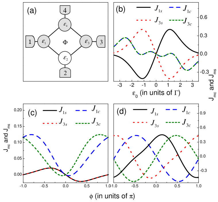
Figure 1: (a) Schematic of a four-terminal four-QD ring structure with a local Rashba interaction on QD-2. Four QDs and the leads coupling to them are denoted as QD-j and lead-j with $j=1-4$. The currents vs the QD levels $\varepsilon_{j}$ as well as the magnetic phase factor $\phi$ are shown in (b) and (c), respectively. The parameter values are $\Gamma_{j}=2\Gamma$ and $\tilde{\alpha}=0.4$. In (b), $\varepsilon_{j}=\varepsilon_{0}$ and $\phi=0$ and in (c), the QD level $\varepsilon_{j}=\Gamma$. (d) The currents vs $\phi$ in the case $\varepsilon_{j}=0$.

The structure under consideration is illustrated in Fig.1(a). In such a system four leads are coupled to their respective QDs in a four-QD ring, with the Rashba effect applied to act locally on QD-2. The single-electron Hamiltonian in this structure can be written as $H_{s}=\frac{\textbf{P}^{2}}{2m^{*}}+V(\textbf{r})+\frac{\hat{y}}{2\hbar}\cdot[\alpha(\hat{\sigma}\times\textbf{p})+(\hat{\sigma}\times\textbf{p})\alpha]$, where the potential $V(\textbf{r})$ confines the electron to form the structure geometry. The last term in $H_{s}$ denotes the local Rashba SO coupling on QD-2. For the analysis of the electron properties, we select the basis set $\{\psi_{jk}\chi_{\sigma},\psi_{j}\chi_{\sigma}\}$($\psi_{j}$ and $\psi_{jk}$ are the orbital eigenstates of the isolated QDs and leads in the absence of Rashba interaction with $j$=1-4; $\chi_{\sigma}$ with $\sigma=\uparrow,\downarrow$ denotes the eigenstates of Pauli spin operator $\hat{\sigma}_{z}$) to second-quantize the Hamiltonian, which is composed of three parts: ${\cal H}_{s}={\cal H}_{c}+{\cal H}_{d}+{\cal H}_{t}$.

$${\cal H}_{c} =\underset{\sigma jk}{\sum}\varepsilon_{jk}c_{jk\sigma}^{\dagger}c_{jk\sigma},$$

$${\cal H}_{d} =\sum_{j=1,\sigma}^{4}\varepsilon_{j}d^{\dagger}_{j\sigma}d_{j\sigma}+\sum_{l=1,\sigma}^{2}[t_{l\sigma}d^{\dagger}_{l\sigma}d_{l+1\sigma}+r_{l}(d_{l\downarrow}^{\dagger}d_{l+1\uparrow}$$

$$-d_{l+1\downarrow}^{\dagger}d_{l\uparrow})]+t_{3}d^{\dagger}_{3\sigma}d_{4\sigma}+t_{4}e^{i\phi}d^{\dagger}_{4\sigma}d_{1\sigma}+\mathrm{H.c.},$$

$${\cal H}_{t} =\underset{\sigma jk}{\sum}V_{j\sigma}d^{\dagger}_{j\sigma}c_{jk\sigma}+\mathrm{H.c.},$$ (1)

where $c_{jk\sigma}^{\dagger}$ and $d^{{\dagger}}_{j\sigma}$ $(c_{jk\sigma}$ and $d_{j\sigma})$ are the creation (annihilation) operators corresponding to the basis in lead-j and QD-j. $\varepsilon_{jk}$ and $\varepsilon_{j}$ are the single-particle levels. $V_{j\sigma}=\langle\psi_{j}\chi_{\sigma}|H|\psi_{jk}\chi_{\sigma}\rangle$ denotes QD-lead coupling strength. The interdot hopping amplitude, written as $t_{l\sigma}=t_{l}-i\sigma s_{l}$($l=1,2$), has two contributions: $t_{l}=\langle\psi_{l}|H_{0}|\psi_{l+1}\rangle$ is the ordinary transfer integral independent of the Rashba interaction; $s_{l}=i\langle\psi_{l}|\alpha p_{x}+p_{x}\alpha|\psi_{l+1}\rangle$, a real quantity for real $\psi_{l}$ and $\psi_{l+1}$, indicates the strength of spin precession. Finally, in the Hamiltonian $r_{l}=\langle\psi_{l}|\alpha p_{z}+p_{z}\alpha|\psi_{l+1}\rangle$ is a complex quantity representing the strength of interdot spin flip. To get an intuitive impression about the typical values of these parameters in the Hamiltonian, we assume that each QD confines the electron by an isotropic harmonic potential ${1\over 2}m^{*}\omega_{0}r^{2}$. Then, the four QDs distribute on a circle equidistantly, and the interval in between is $2l_{0}$($l_{0}=\sqrt{\hbar/m^{*}\omega_{0}}$). Besides, we assume that the electron occupies the ground state in each QD. By defining a dimensionless Rashba coefficient as $\tilde{\alpha}=\alpha/(3\hbar\omega_{0}l_{0})$, we obtain the rough relation of the parameters: $t_{1}=t_{2}$, $s_{1}=s_{2}$, $r_{1}=-r_{2}$, and $|s_{l}|=|r_{l}|\sim\tilde{\alpha}t_{l}$. Thereby we can express the interdot hopping amplitude in an alternative form: $t_{l\sigma}=t_{l}\sqrt{1+\tilde{\alpha}^{2}}e^{-i\sigma\varphi}$ with $\varphi=\tan^{-1}\tilde{\alpha}$. Here the Rashba interaction brings about a spin-dependent phase factor, which can be tuned by varying the electric field strength. In the above Hamiltonian the phase factor $\phi$ attached to $t_{4}$ accounts for the magnetic flux through the ring. In addition, the many-body effect can be readily incorporated into the above Hamiltonian by adding the Hubbard term ${\cal V}_{e\text{-}e}=\sum_{j\sigma}{\frac{U_{j}}{2}}n_{j\sigma}n_{j\bar{\sigma}}$.

Starting from the second-quantized Hamiltonian, we can now formulate the electronic transport properties. With the nonequilibrium Keldysh Green function technique, the current flow in lead-$j$ can be written asMeir

$$J_{j\sigma}=\frac{e}{h}\sum_{j^{\prime}\sigma^{\prime}}\int d\omega T_{j\sigma,j^{\prime}\sigma^{\prime}}(\omega)[f_{j}(\omega)-f_{j^{\prime}}(\omega)],$$ (2)

where $T_{j\sigma,j^{\prime}\sigma^{\prime}}(\omega)=\Gamma_{j}G^{r}_{j\sigma,j^{\prime}\sigma^{\prime}}(\omega)\Gamma_{j^{\prime}}G^{a}_{j^{\prime}\sigma^{\prime},j\sigma}(\omega)$ is the transmission function, describing electron tunneling ability between lead-$j$ to lead-$j^{\prime}$, and $f_{j}(\omega)$ is the Fermi distribution function in lead-$j$. $\Gamma_{j}=2\pi|V_{j\sigma}|^{2}\rho_{j}(\omega)$, the coupling strength between QD-j and lead-j, can be usually regarded as a constant. $G^{r}$ and $G^{a}$, the retarded and advanced Green functions, obey the relationship $[G^{r}]=[G^{a}]^{\dagger}$. From the equation-of-motion method, the retarded Green function can be obtained in a matrix form,

$$[G^{r}]^{-1}=$$

$$\left[\begin{array}[]{cccccccc}g_{1\uparrow}^{-1}&-t_{1\uparrow}&0&-t_{4}e^{-i\phi}&0&r^{*}_{1}&0&0\\ -t^{*}_{1\uparrow}&g_{2\uparrow}^{-1}&-t_{2\uparrow}&0&-r^{*}_{1}&0&r^{*}_{2}&0\\ 0&-t^{*}_{2\uparrow}&g_{3\uparrow}^{-1}&-t_{3}&0&-r^{*}_{2}&0&0\\ -t_{4}e^{i\phi}&0&-t^{*}_{3}&g_{4\uparrow}^{-1}&0&0&0&0\\ 0&-r_{1}&0&0&g_{1\downarrow}^{-1}&-t_{1\downarrow}&0&-t_{4}e^{-i\phi}\\ r_{1}&0&-r_{2}&0&-t^{*}_{1\downarrow}&g_{2\downarrow}^{-1}&-t_{2\downarrow}&0\\ 0&r_{2}&0&0&0&-t^{*}_{2\downarrow}&g_{3\downarrow}^{-1}&-t_{3}\\ 0&0&0&0&-t_{4}e^{i\phi}&0&-t^{*}_{3}&g_{4\downarrow}^{-1}\end{array}\right].$$ (11)

In the above expression, $g_{j\sigma}$ is the Green function of QD-j unperturbed by the other QDs and in the absence of Rashba effect. $g_{j\sigma}=[(z-\varepsilon_{j})\lambda_{j\sigma}+\frac{i}{2}\Gamma_{j}]^{-1}$ with $z=\omega+i0^{+}$ and $\lambda_{j\sigma}=\frac{z-\varepsilon_{j}-U_{j}}{z-\varepsilon_{j}-U_{j}+U_{j}\langle n_{j\bar{\sigma}}\rangle}$ resulting from the second-order approximation of the Coulomb interactionGongprb . $n_{j\sigma}=\langle d^{\dagger}_{j\sigma}d_{j\sigma}\rangle$ can be numerically resolved by iteration technique with $\langle n_{j\sigma}\rangle=-\frac{i}{2\pi}\int d\omega G^{<}_{j\sigma,j\sigma}$.

We now proceed on to calculate the currents in lead-$j$, lead-1 and lead-3 in this case. As for the chemical potentials in respective leads, we consider $\mu_{1}$ as the zero point of energy of this system and $\mu_{1}=\mu_{3}$; $\mu_{2}$ and $\mu_{4}$, the chemical potentials in other two leads, are considered with $\mu_{2}=\mu_{1}+eV/2$ and $\mu_{4}=\mu_{1}-eV/2$, in which $V$ is the bias voltage. The charge and spin currents are defined respectively as $J_{mc}=J_{m\uparrow}+J_{m\downarrow}$ and $J_{ms}=J_{m\uparrow}-J_{m\downarrow}$ ($m=1,3$). Before calculation, we introduce a parameter $\Gamma$ as the unit of energy, the order of which is meV for some experiments based on GaAs/GaAlAs QDs, as mentioned in the previous worksPRL ; PRB .

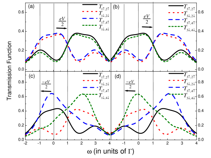
Figure 2: The spectra of transmission functions $T_{m\sigma,m^{\prime}\sigma}$($m$=1,3 and $m^{\prime}$=2,4). (a) and (b) Zero magnetic field case, and (c)-(d) magnetic phase factor $\phi={\pi\over 2}$. The domains of integration to calculate the currents are labeled by the arrows.

To carry out the numerical calculation about the spectra of the charge and spin currents in lead-1 and lead-3, we choose the Rashba coefficient $\tilde{\alpha}=0.4$ which is available in the current experiment.Sarra The structure parameters are taken as $|t_{l\sigma}|=t_{3}=t_{4}=\Gamma$, and the bias voltage is $eV=2\Gamma$. In Fig.1(b), the currents versus the QD levels are shown in the absence of magnetic field. It shows that in the case of the QD levels separate from the energy zero point (i.e., $\varepsilon_{0}\neq 0$), besides the emergence of pure spin currents, a more interesting phenomenon is that the amplitude of $J_{1s}$ is almost the same as that of $J_{3s}$. However, in the case of $\varepsilon_{0}>0$ the value of $J_{1s}$ is greater than zero and $J_{3s}<0$, whereas $J_{1s}<0$ and $J_{3s}>0$ under the condition of $\varepsilon_{0}<0$. This means that, in such a structure applying a finite bias between the longitudinal terminals can efficiently bring out transverse pure spin currents with the opposite polarization directions of them. Moreover, when the QD levels exceed the zero point of energy of the system the polarization directions of these pure spin currents will be thoroughly changed. However, for the case of the QD levels consistent with the zero point of energy, $\varepsilon_{0}=0$, no pure spin current comes about despite a nonzero magnetic flux through the QD ring, as shown in Fig.1(c). When the QD levels take a finite value (eg., $\varepsilon_{0}=\Gamma$), as shown in Fig.1(d), not only there are apparent spin currents in the transverse terminals (lead-1 and lead-3), but also with the adjustment of magnetic flux in either transverse terminal the charge and spin currents oscillate out of phase. In the vicinity of $\phi=(n-{1\over 2})\pi$, $J_{1c}$ and $J_{3c}$ reach their maxima; Simultaneously, the spin current $J_{ms}$ are just at a zero point. On the contrary, when $\phi=n\pi$ the situation is just inverted, the maximum of $J_{ms}$ encounters the zero of $J_{mc}$. In particular, with the change of magnetic phase factor from $\phi=2n\pi$ to $\phi=(2n+1)\pi$ the polarization directions of the transverse pure spin currents are inverted. So, it should be noticed that tuning the QD levels to an nonzero value with respect to the zero point of energy is a key condition of the appearance of transverse pure spin currents.

The calculated transmission functions are plotted in Fig. 2 with $\varepsilon_{j}=\Gamma$. They are just the integrands for the calculation of the charge and spin currents (see Eq.(2)). By comparing the results shown in Figs.2(a) and 2(b), we can readily see that in the absence of magnetic flux, the traces of $T_{1\uparrow,2\uparrow}$, $T_{1\downarrow,4\downarrow}$, $T_{3\downarrow,2\downarrow}$, and $T_{3\uparrow,4\uparrow}$ coincide with one another very well, so do the curves of $T_{1\downarrow,2\downarrow}$, $T_{1\uparrow,4\uparrow}$, $T_{3\uparrow,2\uparrow}$, and $T_{3\downarrow,4\downarrow}$. Substituting such integrands into the current formulae, one can certainly arrive at the result of the distinct pure spin currents, which flows from lead-1 to lead-3 in such a case. On the other hand, these transmission functions depend nontrivially on the magnetic phase factor, as exhibited in Fig.2(c) and (d) with $\phi={\pi\over 2}$. In comparison with the zero magnetic field case, herein the spectra of $T_{m\sigma,2\sigma}$ are reversed about the axis $\omega=\Gamma$ without the change of their amplitudes, but $T_{m\sigma,4\sigma}$ only present the enhancement of their amplitudes. Similarly, with the help of Eq.(2), one can understand the disappearance of spin currents in such a case.

The underlying physics being responsible for the spin dependence of the transmission functions is quantum interference, which manifests if we analyze the electron transmission process in the language of Feynman path. Notice that the spin flip arising from the Rashba interaction does not play a leading role in causing the appearance of spin and charge currentsGong-APL . Therefore, to keep the argument simple, we drop the spin flip term for the analysis of quantum interference. With this method, we write $T_{1\sigma,2\sigma}=|\tau_{1\sigma,2\sigma}|^{2}$ where the transmission probability amplitude is defined as $\tau_{1\sigma,2\sigma}=\widetilde{V}^{*}_{1\sigma}G^{r}_{1\sigma,2\sigma}\widetilde{V}_{2\sigma}$ with $\widetilde{V}_{j\sigma}=V_{j\sigma}\sqrt{2\pi\rho_{j}(\omega)}$. By solving $G^{r}_{1\sigma,2\sigma}$, we find that the transmission probability amplitude $\tau_{1\sigma,2\sigma}$ can be divided into three terms, i.e., $\tau_{1\sigma,2\sigma}=\tau^{(1)}_{1\sigma,2\sigma}+\tau^{(2)}_{1\sigma,2\sigma}+\tau^{(3)}_{1\sigma,2\sigma}$, where $\tau^{(1)}_{1\sigma,2\sigma}=\frac{1}{D}\widetilde{V}^{*}_{1\sigma}g_{1\sigma}t_{1\sigma}g_{2\sigma}\widetilde{V}_{2\sigma}$, $\tau^{(2)}_{1\sigma,2\sigma}=\frac{1}{D}\widetilde{V}^{*}_{1\sigma}g_{1\sigma}t_{4}e^{-i\phi}g_{4\sigma}t^{*}_{3}g_{3\sigma}t^{*}_{2\sigma}g_{2\sigma}\widetilde{V}_{2\sigma}$, and $\tau^{(3)}_{1\sigma,2\sigma}=-\frac{1}{D}\widetilde{V}^{*}_{1\sigma}g_{1\sigma}t_{1\sigma}g_{2\sigma}t_{2\sigma}g_{3\sigma}t^{*}_{2\sigma}g_{2\sigma}\widetilde{V}_{2\sigma}$ with $D=\det\{[G^{r}]^{-1}\}\prod_{j}g_{j\sigma}$. By observing the structures of $\tau^{(1)}_{1\sigma,2\sigma}$, $\tau^{(2)}_{1\sigma,2\sigma}$, and $\tau^{(3)}_{1\sigma,2\sigma}$, we can readily find that they just represent the three paths from lead-2 to lead-1 via the QD ring. The phase difference between $\tau^{(1)}_{1\sigma,2\sigma}$ and $\tau^{(2)}_{1\sigma,2\sigma}$ is $\Delta\phi^{(1)}_{2\sigma}=[\phi-2\sigma\varphi-\theta_{3}-\theta_{4}]$ with $\theta_{j}$ arising from $g_{j\sigma}$, whereas the phase difference between $\tau^{(2)}_{1\sigma,2\sigma}$ and $\tau^{(3)}_{1\sigma,2\sigma}$ is $\Delta\phi^{(2)}_{2\sigma}=[\phi-2\sigma\varphi]$. It is clear that only these two phase differences are related to the spin polarization. $T_{1\sigma,4\sigma}$ can be analyzed in a similar way. We then write $T_{1\sigma,4\sigma}=|\tau^{(1)}_{1\sigma,4\sigma}+\tau^{(2)}_{1\sigma,4\sigma}+\tau^{(3)}_{1\sigma,4\sigma}|^{2}$, with $\tau^{(1)}_{1\sigma,4\sigma}=\frac{1}{D}\widetilde{V}^{*}_{1\sigma}g_{1\sigma}t_{4}e^{-i\phi}g_{4\sigma}\widetilde{V}_{4\sigma}$, $\tau^{(2)}_{1\sigma,4\sigma}=\frac{1}{D}\widetilde{V}^{*}_{1\sigma}g_{1\sigma}t_{1\sigma}g_{2\sigma}t_{2\sigma}g_{3\sigma}t_{3}g_{4\sigma}\widetilde{V}_{4\sigma}$, and $\tau^{(3)}_{1\sigma,4\sigma}=-\frac{1}{D}\widetilde{V}^{*}_{1\sigma}g_{1\sigma}t_{4}e^{-i\phi}g_{4\sigma}t^{*}_{3}g_{3\sigma}t_{3}g_{4\sigma}\widetilde{V}_{4\sigma}$. The phase difference between $\tau^{(1)}_{1\sigma,4\sigma}$ and $\tau^{(2)}_{1\sigma,4\sigma}$ is $\Delta\phi^{(1)}_{4\sigma}=[\phi-2\sigma\varphi+\theta_{2}+\theta_{3}]$, and $\Delta\phi^{(2)}_{4\sigma}=[\phi-2\sigma\varphi]$ originates from the phase difference between $\tau^{(2)}_{1\sigma,4\sigma}$ and $\tau^{(3)}_{1\sigma,4\sigma}$. Utilizing the parameter vlues in Fig.2, we evaluate that $\varphi\approx{\pi\over 7}$ and $\theta_{j}=-\frac{3\pi}{4}$ at the point of $\omega=0$. It is apparent that when $\phi=0$ only the phase differences $\Delta\phi^{(1)}_{2\sigma}$ and $\Delta\phi^{(1)}_{4\sigma}$ are spin-dependent. Accordingly, we obtain that $\Delta\phi^{(1)}_{2\uparrow}=-\Delta\phi^{(1)}_{4\downarrow}={17\pi\over 14}$, and $\Delta\phi^{(1)}_{2\downarrow}=-\Delta\phi^{(1)}_{4\uparrow}=-{3\pi\over 14}$, which clearly prove that the quantum interference between $\tau^{(1)}_{1\uparrow,2\uparrow}$ and $\tau^{(2)}_{1\uparrow,2\uparrow}$ ($\tau^{(1)}_{1\downarrow,4\downarrow}$ and $\tau^{(2)}_{1\downarrow,4\downarrow}$ alike) is destructive, but the constructive quantum interference occurs between $\tau^{(1)}_{1\downarrow,2\downarrow}$ and $\tau^{(2)}_{1\downarrow,2\downarrow}$ ($\tau^{(1)}_{1\uparrow,2\uparrow}$ and $\tau^{(2)}_{1\uparrow,2\uparrow}$ alike). Then such a quantum interference pattern can explain the traces of the transmission functions shown in Fig.2(a). In the case of $\phi=\frac{1}{2}\pi$ we find that only $\Delta\phi^{(2)}_{2(4)\sigma}$ are crucial for the occurrence of spin polarization. By a calculation, we obtain $\Delta\phi^{(2)}_{2(4)\uparrow}={5\pi\over 14}$ and $\Delta\phi^{(2)}_{2(4)\downarrow}={9\pi\over 14}$, which are able to help us clarify the results in Fig.2(c) and (d). Up to now, the characteristics of the transmission functions, as shown in Fig.2, hence, the tunability of charge and spin currents have been clearly explained by analyzing the quantum interference between the transmission paths.

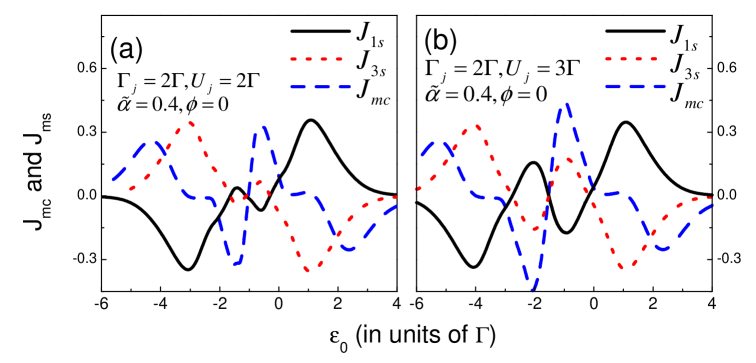
Figure 3: The currents versus $\varepsilon_{0}$ in the presence of many-body terms with $U_{j}=2\Gamma$ and $3\Gamma$, respectively.

So far we have not discuss the effect of electron interaction on the occurrence of pure spin currents, though it is included in our theoretical treatment. Now we incorporate the electron interaction into the calculation, and we deal with the many-body terms by employing the second-order approximation, since we are not interested in the electron correlation here. Figure 3 shows the calculated currents spectra with $U_{j}=2\Gamma$ and $3\Gamma$, respectively. Clearly, within such an approximation the Rashba-induced transverse pure spin currents remain, though the current spectra oscillate to a great extent with the shift of QD levels.

In conclusion, by introducing a local Rashba interaction on an individual QD, we have studied the electronic transport through a four-QD ring with four terminals. As a consequence, the Rashba-induced transverse pure spin currents are observed by applying a finite bias on the longitudinal terminals. The modulation of the QD levels and the magnetic phase factor can efficiently adjust the phases of the transmission paths, thus the spin-dependent electron transmission probabilities can be controlled by tuning these structure parameters, which brings out the change of the amplitudes and directions of the pure spin currents. With respect to the quantum interference in such a structure, we have to illustrate two aspects. First, the applying of Rashba interaction is the precondition of the spin-dependent electron transmission. The presence of the multi-terminal configuration leads to the comparative amplitudes of the different transmission paths for the quantum interference. Finally, it should be emphasized that altering the longitudinal bias, equivalent to interchange the sequence numbers of lead-1 and lead-3, can also change the polarization directions of the pure spin currents.

References

(1) S. Datta and B. Das, Appl. Phys. Lett. 56, 665 (1990).
(2) S. A. Wolf, ., Science 294, 1488 (2001);
Zutic, J. Fabian, and S. Das Sarma, Rev. Mod. Phys. 76, 323
(2004).
(3) A. Bychkov and E. I. Rashba,
J. Phys. C 17, 6039 (1984); J. Nitta, T. Akazaki, H.
Takayanagi, and T. Enoki, Phys. Rev. Lett. 78, 1335 (1997).
(4) J. E. Hirsch, Phys. Rev. Lett. 83, 1834 (1999).
(5) J. Sinova, Phys. Rev. Lett. 92, 126603 (2004).
(6) E. G. Mishchenko, A.V. Shytov, and B. I. Halperin, Phys. Rev.
Lett. 93, 226602 (2004).
(7) I. Žutić, J. Fabian, and S. Das Sarma, Appl. Phys. Lett.
82, 221 (2003); G. Schmidt, D. Ferrand, L. W. Molenkamp, A.
T. Filip, and vanWees B. J., Phys. Rev. B 62, R4790 (2000).
(8) D. V. Bulaev and D. Loss, Phys. Rev. B 71,
205324 (2005).
(9) B. K. Nikolic and S. Souma, Phys. Rev. B 71,
195328 (2005).
(10) S. Murakami, N. Nagaosa, and S.-C. Zhang, Science 301,
1348 (2003).
(11) J. H. Bardarson, İ. Adagideli, and Ph. Jacquod, Phys. Rev. Lett. 98, 196601
(2007).
(12) Q. F. Sun, J. Wang, and H. Guo, Phys. Rev. B 71,
165310 (2005); Q.F. Sun and X. C. Xie, Phys. Rev. B 73,
235301 (2006).
(13) F. Chi and S. Li, J. Appl. Phys. 100, 113703 (2006).
(14) H. F. Lü and Y. Guo, Appl. Phys. Lett. 91,
092128(2007); F. Chi and J. Zheng, Appl. Phys. Lett. 92,
062106(2008).
(15) W. Gong, Y. Zheng, and
T. Lü, Appl. Phys. Lett. 92, 042104 (2008).
(16) Y. Meir and N. S. Wingreen, Phys. Rev. Lett. 68, 2512 (1992);
A.-P. Jauho, N. S. Wingreen, and Y. Meir, Phys. Rev. B 50,
5528 (1994).
(17) J. Q. You and H. Z. Zheng, Phys. Rev. B 60, 13314 (1999); W. Gong, Y. Zheng,Y. Liu and
T. Lü, Phys. Rev. B 73, 245329 (2006).
(18) M. Sigrist, T. Ihn, K. Ensslin, M. Reinwald, and W. Wegscheider,
Phys. Rev. Lett. 98, 036805 (2007).
(19) V. I. Puller and Y. Meir, Phys. Rev. B
77, 165421 (2008).
(20) J. Nitta, T. Akazaki, H. Takayanagi, and T. Enoki, Phys. Rev. Lett. 78,
1335 (1997); F. Mireles and G. Kirczenow, Phys. Rev. B 64,
024426 (2001); D. Sánchez and L. Serra, Phys. Rev. B
74, 153313 (2006).