Monte Carlo simulations on rare-earth Holmium ultra-thin films

Abstract

Motivated by recent experimental results in ultra-thin helimagnetic Holmium films, we have performed an extensive classical Monte Carlo simulation of films of different thickness, assuming a Hamiltonian with six inter-layer exchange constants. Both magnetic structure and critical properties have been analyzed. For $n>16$ ($n$ being the number of spin layers in the film) a correct bulk limit is reached, while for lower $n$ the film properties are clearly affected by the strong competition among the helical pitch and the surface effects, which involve the majority of the spin layers: In the thickness range $n=9\div 16$ three different magnetic phases emerge, with the high-temperature, disordered, paramagnetic phase and the low-temperature, long-range ordered one separated by an intriguing intermediate-temperature block phase, where outer ordered layers coexist with some inner, disordered ones. The phase transition of these inner layers displays the signatures of a Kosterlitz-Thouless one. Finally, for $n\lesssim 7$ the film collapse once and for all to a quasi-collinear order. A comparison of our Monte Carlo simulation outcomes with available experimental data is also proposed, and further experimental investigations are suggested.

I Introduction

Surface and nanometrical objects are important both for their possible implementation in the current technology and from basic research point of view. In collinear magnetic thin films intriguing behavior, as transition temperature depending from the film thickness $-n-$ or critical exponent crossover, were observed Fisher72 ; Ritchie ; Barber ; Henkel99 ; Henkel98 ; zhang01 .

Nowadays, the most fervent interest has moved towards frustrated systems, where a non-collinear order, characterized by a possibly large modulation, is established. Some rare-earth elements (as Holmium, Dysprosium or Terbium) and their compounds are typical examples that the nature makes available to investigate such peculiar behaviours, in view of the variety of magnetic arrangements, as helix, spiral or longitudinal-wave, that can be observed in bulk samples of such materials.Jensen91 . Further examples of helicoidal structures can also be met in multiferroic materialsmf1 ; mf2 ; mf3 and itinerant systems, as MnSi MnSi and FeGe FeGe .

In magnetic systems with frustration, the lack of translational invariance due to the presence of surfaces can result especially important for ultra-thin film samples where the thickness is comparable, or even lower, with the wave length of the ordered magnetic structure observed in the bulk. It is worthwhile observing that when these conditions are met a sweeping change of the magnetic structure behaviour could be found. Many fundamental features related to such systems have not yet been exhaustively investigated and completely understood, and ultra-thin films of rare-earth elements are still among the most intriguing layered systems to be studiedJensen05 .

From an experimental point of view, the availability of new sophisticated growth and characterization techniquesBland has allowed to extensively investigate the properties of such magnetic nano-structures. For instance, interesting experimental data on thin films of Holmium (whose bulk samples show helical order along the $c$ axis, perpendicular to film basal planes) were obtained Weschke04 ; Weschke05 ; Jensen05 ; schss00 by neutron diffraction and resonant soft X-ray experiments. By looking at the static structure factor $S(\vec{Q})$ ($\vec{Q}=(0,0,Q_{z})$ being the wave vector of the incommensurate magnetic modulation along the film growth direction $z$), it has been shown that the critical behaviour of Holmium thin films markedly differ from that of films of transition metals, which usually display a collinear ferromagnetic (FM) or antiferromagnetic (AFM) order in the bulk. Mainly, the authors of Refs. Weschke04, ; Weschke05, ; Jensen05, ; schss00, identified a thickness $n_{0}\simeq 10$ mono-layers [ML] (comparable with the helix pitch of bulk Holmium $\simeq 12$ ML) which was interpreted as a lower bound for the presence of the helical ordered phase. In fact, they observed that the transition temperature dependence on film thickness does not follow the usual asymptotic power law Barber , but rather an empirical relation

$$\frac{T_{N}(\infty)-T_{N}(n)}{T_{N}(n)}\sim\frac{1}{(n-n_{0})^{\lambda^{\prime}}}~{},$$ (1)

can be devised Weschke04 , where $T_{N}(\infty)$ and $T_{N}(n)$ are the ordering temperature of the bulk system and of a film with thickness $n$, respectively, while the exponent $\lambda^{\prime}$ has not an universal character. Interesting enough, it appears that this empirical relation is not peculiar of helical-like structures only but it results more general, being observed in other ultra-thin structures characterized by a magnetic modulation as well: An important example is given by Chromium films, where at low temperatures an incommensurate spin density wave is present Fullerton95 .

A mean field approximation (MFA) was proposed in Refs. Jensen05, and Weschke04, in order to understand the experimental outcomes from Holmium films: MFA allowed to obtain a first, rough estimate of the threshold thickness $n_{0}$ defined in the empirical relation (1), but it also revealed that for thicknesses close enough to $n_{0}$ the paramagnetic and helical phase can be accompanied by a more complex block phase, where groups of ferromagnetically ordered layers pile-up in an alternating antiferromagnetic arrangement along the c axis. As it is well known, the MFA completely neglects thermal fluctuations, which are however strongly expected to play a fundamental role in the critical behaviour of low-dimensional magnetic systems: therefore, adding thermal fluctuations not only give strong quantitative adjustments of the MFA estimates of critical quantities as $T_{N}(n)$ or $n_{0}$, but could also make unstable some ordered structure as the block phase met above.

In order to overcome such issues and deepen our understanding of critical phenomena in Holmium ultra-thin films, we performed extensive classical Monte Carlo Simulations (MCS): Preliminary results already showed Cinti1 that thermal fluctuations do not destroy the block phase, which instead acquire a much richer structure, with disordered inner layers intercalating ordered ones and undergoing a Kosterlitz-Thouless (KT) phase transitionKTt as the temperature lowers.

A complete account is here given of the results of our simulations for film thickness in the range $n=6\ldots 36$ ML. The paper is organized as follows: In Sec. II we shall briefly recall relevant properties of Holmium, and introduce the magnetic model Hamiltonian. Sec. III is devoted to describe the Monte Carlo method and the estimators employed to evaluate the physical quantities relevant for magnetic films with non-collinear order. In Sec. IV the Monte Carlo results about the magnetic order establishing at low temperature are shown for different thicknesses. The role of thermal fluctuations is discussed in Sec. V: In particular, Sec. V.1 will report a detailed study of the temperature regions where the single layers display a critical behaviour, the structure factor close to these regions being deeply analyzed too, given its fundamental relevance in an experimental mindset; Sec. V.2 will be devoted to the global film properties. All the results reported in the previous sections will be compared and discussed in an unifying framework in Sec. VI, where we shall also gather our conclusions.

II Model Hamiltonian

The magnetic properties of Holmium have been intensively investigated both experimentally and theoretically Jensen91 . The bulk crystal structures is known to be hexagonal close-packed (hcp). The indirect exchange among the localized 4f electrons manifests as an RKKY long-range interaction of atomic magnetic moments; the experimental data about the low-temperature magnetic moments arrangement in Ho can be reproduced assuming a FM interaction between nearest neighbor spins lying on the ab crystallographic planesJensen91 , while along the c crystallographic axis interactions up to the sixth neighboring layers must be allowed for (see for example Ref. Borh89, ). It’s just the competing nature of the latter that below $T_{N}(\infty)=132$ K gives rise to an incommensurate magnetic periodic structure, which can be modeled as an helical arrangement of the magnetic moment vectors along the direction (henceforth denoted as z) parallel to c, i.e. perpendicular to the ab crystallographic planes, where the magnetic vectors prefer to lye as a consequence of a single-ion easy-plane anisotropy. The average local spin vector at low temperature can thus be expressed as:

$$\vec{s}_{i}\equiv\vec{s}\left(\vec{r}_{i}\right)=\left(s_{\perp}\cos\left(\vec{Q}\cdot\vec{r}_{i}\right),s_{\perp}\sin\left(\vec{Q}\cdot\vec{r}_{i}\right),s_{z}\right)~{},$$ (2)

where $\vec{Q}=\left(0,0,Q_{z}^{bulk}\right)$ is the helical pitch vector, and $c\,Q_{z}^{bulk}\simeq\pi/3$, c being the lattice constant Jensen91 along the z direction (i.e., $c/2$ is the distance between nearest neighbouring ab spin layers). In addition, the crystal field bring into play other different kinds of anisotropies that, at temperatures well below $T_{N}(\infty)$, are able to change the helical shapes in conical ones, or force the magnetic structures in a bunched helix which is commensurate with the lattice Gibbs85 ; Jensen87 .

Theoretical investigations have shown that incommensurate magnetic bulk structures (observed, besides Holmium, also in other rare-earth elements, as Dysprosium and Terbium) can be well obtained by a MFA Coqblin77 from a simple Heisenberg model with only three coupling constant, the first one, $J_{0}>0$, describing the FM in-plane interactions, while $J_{1}$ and $J_{2}$ are the effective coupling between ions on neighbouring (NN) and next-neighbouring (NNN) planes, respectively. Whatever the sign of $J_{1}$, the MFA finds a helical structure when $J_{2}<0$, i.e. AFM, and the conditions $|J_{2}|>|J_{1}|/4$ is met.

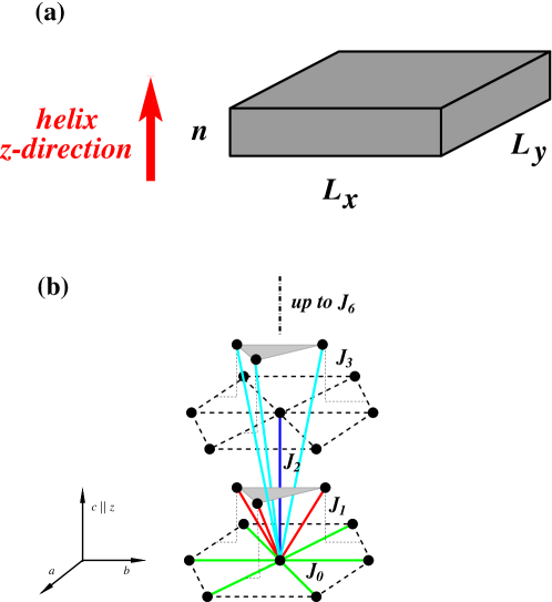
Figure 1: (color online) (a) Film geometry: $N=n\times L_{x}\times L_{y}$ is the total number of spins, $n$ is the film thickness, i.e. the number of spin layer (free boundary conditions are taken along $z$-direction), and $L_{x,y}$ are the layer dimensions (periodic boundary conditions are applied along $x$ and $y$ directions). (a) Schematic representation of hcp Ho structure and exchange interactions: only $J_{0}$ (in-plane, green lines), $J_{1}$ (NN planes, red lines), $J_{2}$ (NNN planes, blue line), and $J_{3}$ (cyan lines) are represented. The numerical values of the coupling constants employed in our simulations are: $J_{0}=55.68$ K, $J_{1}=24.9168$ K, $J_{2}=5.4288$ K, $J_{3}=-3.3686$ K, $J_{4}=-4.5936$ K, $J_{5}=-0.2784$ K, $J_{6}=-2.5056$ K.

It is worthwhile to recall that when dealing with ultra-thin films the assumption of being allowed to retain the same Hamiltonian able to describe the bulk structure is absolutely not guaranteed to be correct: Indeed, real film samples can be strongly affected by defects, strain, thickness uncertainty ($\sim$2 ML) or interaction with the substrate comm (typically Y/Nb or W(110)). The latter can be particularly relevant, as it can change, sometimes dramatically, the single ion anisotropy and the strength of the interaction constants with respect to bulk samples. Furthermore, the lack of inversion symmetry can bring into play the antisymmetric Dzyaloshinskii-Moriya (DM) interaction moriya60 (see for instance Ref. Dagotto06, and Mostovoy06, for perovskite multiferroic RMnO₃ with R = Gd, Tb, or Dy) and possible surface anisotropies for Dy/Y multilayer films super .

While always remembering such possible drawbacks, in our investigation of Ho thin films we employ a Heisenberg model Hamiltonian which has proven useful to describe Holmium bulk samples. We thus define:

$${\cal H}=-\sum_{i,j}^{N}J_{ij}\vec{\sigma}_{i}\cdot\vec{\sigma}_{j}+D_{z}\sum_{k=1}^{N}\left(\sigma^{z}_{k}\right)^{2}~{},$$ (3)

where $N=n\times L_{x}\times L_{y}$ is the total number of magnetic ions, $L_{x}=L_{y}=L$ being the lateral film dimensions and $n$ the number of layers (see Fig. 1a), and $\vec{\sigma}_{i}$ are classical unitary vectors representing the total angular momentum of Ho ions (i.e. $\vec{\sigma}_{i}=\vec{\mathcal{J}}_{i}/|\vec{\mathcal{J}}_{i}|$). As a consequence, the magnitude of the angular momentum of Ho ions is embodied in our definition of the coupling constants appearing in Eq. (3) as $J_{ij}=\frac{1}{2}|\vec{\mathcal{J}}|(|\vec{\mathcal{J}}|+1)\textsc{J}_{ij}$, with $|\vec{\mathcal{J}}_{i}|=8$. For the inter-layer exchange parameters $\textsc{J}_{ij}$ we have assumed the values given in Ref. Borh89, , while the easy plane anisotropy $D_{z}=16$ K Coqblin77 .

In Fig. 1b we show a schematic representation of the hcp lattice structure and of the exchange interactions included in the model Hamiltonian (3). On the hexagonal basal planes only a NN, FM interaction $J_{0}>0$ (green lines) is considered; along the $c$-axis we instead allow for interactions up to the sixth neighboring layer, with a total coordination number $\zeta=30$.

Sign and magnitude of the out-of-plane interaction constants J₁ … J₆ were determined in Ref. Borh89, in order to reproduce, with the correct pitch vector, the helical ground state along the c-axis observed in the experimental data. However, at the best of our knowledge, also neutron scattering experiments investigated the dynamical properties of Holmium only along the $c$-axis Jensen87 , so that a direct measure of the in plane FM coupling constant is still lacking, and only mean field estimates are available, which set it at about 300$\mu$eV Weschke04 . This allows us to consider J₀ as an almost free fit parameter to be adjusted in order to fix the correct value of experimentally accessible quantities. By Monte Carlo simulations we find the value $T_{N}^{\textnormal{MCS}}(\infty)\simeq 124$ K for the bulk ordering temperature by setting J${}_{0}\approx 400$ $\mu$eV: bearing in mind the cautions given above about the possible quantitative difference among bulk and film samples, this is the value of J₀ we have used in all the following simulations of thin films, without attempting any further possibly meaningless quantitative adjustment.

III Monte Carlo Methods and Thermodynamic Observables

Our study of the magnetic properties of thin rare earth films was done by extensive classical MCS. Thickness n from 6 to 36 and lateral dimensions $L_{x}=L_{y}=L=8\ldots 80$ have been analyzed. As we are working on film structures, free boundary conditions in the thickness direction $z$ are obviously taken, while the usual periodic boundary conditions are applied in the $L\times L$ planes (see Fig. 1a), which coincide both with the ab crystallographic planes and the easy plane for the magnetization.

Simulations were done at different temperatures; the thermodynamic equilibrium is reached by the usual Metropolis algorithm met53 and over-relaxed technique over87 . The latter was employed in order to speed-up the sampling of the whole spin configuration space: Indeed, the competitive nature of the exchange interactions in the Hamiltonian (3) and the high coordination number lead to a long time needed to reach thermal equilibrium, especially in the critical region. We have thus resorted to a judicious mix of Metropolis and over-relaxed moves in order to reach the goal in a reasonable time. Usually, one “Monte Carlo step” is composed by one Metropolis and four/five over-relaxed moves per particle, discarding up to 5$\times$10⁴ Monte Carlo steps for thermal equilibration; at least three independent simulations where done for for each temperature.

The Monte Carlo data analysis have benefited from the employment of the multiple histogram technique Ferrenberg88 ; bootstrap , which allows us to estimate the physical observables of interest over a whole temperature range by interpolating the results obtained from simulations performed at some chosen, different temperatures. The outcome of the method is an estimate of the density of state $\rho(\mathcal{E})$ at energy $\mathcal{E}$ obtained by weighting the contributes $\rho_{i}(\mathcal{E})$ due to independent simulations made at inverse temperature $\beta_{i}$ ($\beta_{i}=1/k_{B}T_{i}$). The independent simulations have to be sufficiently close in temperature, i.e. the temperature step must be chosen roughly proportional to the square root of the inverse of the heat capacity bootstrap . We thus have computed the partition function $\mathcal{Z}_{\beta}$ at any $\beta$ in the range of interest by solving iteratively the equation

$$\mathcal{Z}_{\beta}=\sum_{\mathcal{E}}\rho(\mathcal{E})\textnormal{e}^{-\beta\mathcal{E}}=\sum_{i,s}\left[\sum_{k}\frac{m_{k}}{\mathcal{Z}_{\beta_{k}}}\textnormal{e}^{\Delta\beta_{k}\mathcal{E}_{i,s}}\right]^{-1}~{},$$ (4)

where $\Delta\beta_{k}=\beta-\beta_{k}$ and $m_{k}$ is the number of independent samples of energy for the $k$-simulation. The index $i$ refers again to the single simulation, while $s$ denotes the energy sampling intervals in the $i$-th simulation.

As mentioned above, the high number of exchange interactions makes difficult the estimate of the density of state, especially close to the critical temperature, and variables like specific heat or susceptibility are extremely sensitive for these systems. Anyway, this obstacle has been successfully overcome making use of the estimator,

$$C_{v}=\frac{\beta^{2}}{N}\langle\left(\mathcal{E}-\langle\mathcal{E}\rangle_{\beta}\right)^{2}\rangle_{\beta}$$ (5)

in the histogram reweighting techniques, as suggested in Ref.PRElandau, . Iterating several times the multiple-histogram algorithm, we have also obtained the variance of the interpolated data by bootstrap resampled method, by picking out randomly a sizable number of independent measurements $m_{k}$ (between 1 and 5$\times$10⁴), and iterating the re-sampling at least one hundred times bootstrap ; bootstrap1 .

As we are interested in the phase transitions of Holmium films, it is worthwhile to observe that the study of films described by the Hamiltonian (3) entails a wide number of fundamental issues. First of all we must consider: i) the intrinsically two-dimensional (2d) nature of such magnetic structures; ii) the presence of different interactions, which turn out to be FM on the layers (with a SO(2) symmetry) and competitive along the thickness direction n, with a possible helimagnetic (HM) order at low temperature (i.e. a $\mathbb{Z}_{2}$ $\times$SO(2) symmetry Kawamura ); and iii) the implementation of different boundary conditions for n and L, respectively, above introduced.

About the first issue, it is well known that the critical behaviour of an ideal easy-plane magnetic film with continuous symmetry and short-range FM (or AFM) interactions pertains to the 2d XY universality class, displaying a KT behaviour KTt at a finite critical temperature. In particular, a crossover from 3d to 2d behaviour is expected when the correlation length saturates the film thickness. However, from MCS point of view, it may result quite difficult to realize such conditions. Indeed, even for large, but still finite, $L$ values a sharp transition can not be observed, making it possible to define a 3d pseudo critical point, as extensively discussed by Janke and co-workers in Refs. Janke93a, ; Janke93b, .

Turning to the second issue, in a quasi-2d magnetic system with a continuous symmetry the introduction of competing interactions along the direction perpendicular to the film slab brings into play the presence of two (in-plane and out-of-plane) correlation lengths, with a rather dissimilar behaviour in the critical regime. As analyzed in Ref. Cinti1, , under these conditions some new and interesting critical phenomena can be observed. Systems with discrete symmetries which present two different correlation lengths were already discussed in literature, see, e.g., Refs. wang89, and bunker93, .

Moving to the last issue, we must first of all observe that the identification of a suitable order parameter to study the critical properties of non-collinear thin films requires a careful analysis of some of their peculiar features. A first trouble is the intrinsic difficulty represented by a helical order parameter associated to a wave vector $\vec{Q}$: In the bulk system the virtually infinite size of the system, summing up an infinite number of in-phase contributions, makes a clear peak emerge at wave-vector $\vec{Q}$ in the static structure factor in the ordered phase. In films, the presence of broad peaks is on the contrary expected in a wide temperature range as, a consequence of the intrinsic finite size nature of the system, thus jeopardizing the identification of a well defined critical temperature $T_{N}(n)$ from the sole analysis of the peaks appearing in the structure factor. Secondly, as we will discuss in the next Sections, a naïve structure factor analysis could be not enough to distinguish between an HM order and other ordered phases that can be present. For these reasons, it is necessary to resort to other observables related to the HM order. A first choice can be found in the chirality Diep94 ; Cinti2 , which can be defined on film as:

$$\kappa=\frac{1}{3(n-1)L^{2}\sin Q_{z}^{bulk}}\sum_{li}\left(\vec{\sigma}_{l,i}\times\vec{\sigma}_{l+1,i}\right)^{z}~{},$$ (6)

where $l$ labels the planes, starting from one of the two film surfaces, and $i$ locates the spin on the plane. As we shall see in the next Sections $\kappa$ represents quite a good quantity to locate the critical temperature for the HM phase. In view of point i) discussed above, it is useful to introduce a FM order parameter for each layer $l$:

$$M_{l}=\sqrt{(M^{x}_{l})^{2}+(M^{y}_{l})^{2}+(M^{z}_{l})^{2}}~{},$$ (7)

where $M^{\alpha}_{l}=\frac{1}{L^{2}}\sum_{i}\sigma^{\alpha}_{l,i}$, with $\alpha=x,y,z$, and consequently the average order parameter of the film Loison00a ; Loison00b :

$$M=\frac{1}{n}\sum_{l}^{n}M_{l}~{}.$$ (8)

It is worth to observe that the order signalled by the quantities defined in Eq. (7) and (8) do not directly entail the existence of an HM or fan structure in the film.

The critical nature of the observables defined in Eqs. (6), (7), and (8), is better revealed by looking at the following derived quantities ($\mathcal{O}=\kappa,M_{l},M$):

$$\langle\chi_{\mathcal{O}}\rangle=N\beta\left(\langle\mathcal{O}^{2}\rangle-\langle\mathcal{O}\rangle^{2}\right)~{},$$ (9)

$$\frac{\partial}{\partial\beta}\langle\mathcal{O}\rangle=\langle\mathcal{OE}\rangle-\langle\mathcal{O}\rangle\langle\mathcal{E}\rangle~{},$$ (10)

$$\frac{\partial}{\partial\beta}\langle\ln\mathcal{O}\rangle=\frac{\langle\mathcal{OE}\rangle}{\langle\mathcal{E}\rangle}-\langle\mathcal{O}\rangle\langle\mathcal{E}\rangle~{},$$ (11)

which, at the critical temperature, display a peak that can be characterized by the usual finite size scaling theory Libbinder . In particular, for large enough $L$, $T_{N}^{L}(n)$ approximately scales as

$$T_{N}^{L}(n)\approx T_{N}^{\infty}(n)+CL^{-1/\nu}~{},$$ (12)

where $C$ is system dependent constant, while $\nu$ is the correlation length critical exponent.

A final quantity we employ in our investigation of the critical properties of films is the Binder cumulant binderu4 ; binderprl :

$$U_{4}=1-\frac{\langle\mathcal{O}^{4}\rangle}{\langle\mathcal{O}^{2}\rangle^{2}}~{},$$ (13)

which allows us to locate the critical temperature by looking at the intersection of the graphs of $U$ as a function of $T$ obtained at different $L$: At $T=T_{N}(n)$ such crossing becomes a “nontrivial fixed-point” binderu4 ; binderprl . Moreover, one can examine the ratios $U_{L^{\prime}}/U_{L}$ (for sizes $L$ and $L^{\prime}>L$) as temperature function, looking for a unitary ratio at the critical temperature.

IV Magnetic Structures at low Temperature

In this section we will present and analyze our Monte Carlo results for the overall magnetic behaviour of film samples of different thicknesses, from a bulk-like structure with $n=36$ to a very thin film of $n=6$ layers, at temperature $T=10$ K, i.e. well below $T_{N}(n)$; the lateral dimension of the films is taken constant at $L=80$, having checked that at this temperature, far from the critical region, such value of $L$ well represents the thermodynamic limit for all practical purpose.

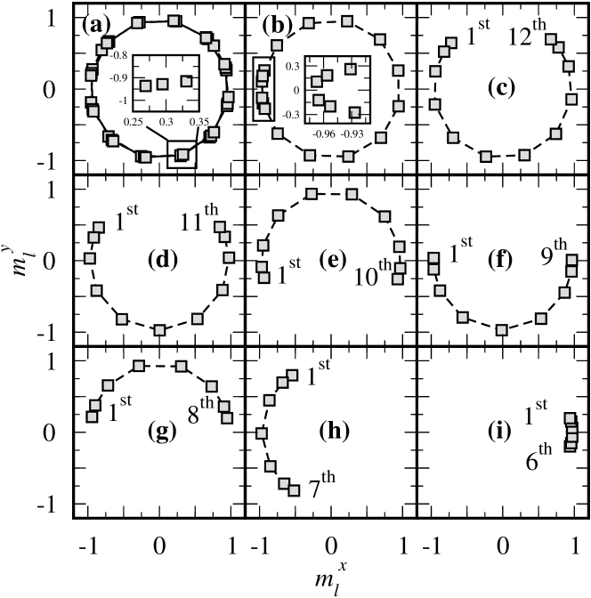
Figure 2: Normalized magnetic vector profiles of each layer at $T=10$ K, layer dimensions $L_{x,y}=80$ and different film thickness $n$: (a) $n=36$; (b) $n=16$; (c) $n=12$; (d) $n=11$; (e) $n=10$; (f) $n=9$; (g) $n=8$; (h) $n=7$; (i) $n=6$; the error bars are included in point dimensions. Inset in (a): the magnified zone of the main graph (here shown for the 6${}^{\textnormal{th}}$, 18${}^{\textnormal{th}}$, and 30${}^{\textnormal{th}}$ planes from left to right along $m_{l}^{x}$, respectively) clearly shows that the helix pitch and lattice structure are incommensurate; inset in (b): the magnification shows the magnetization of the first surface layers: 1${}^{\textnormal{st}}$, 14${}^{\textnormal{th}}$, 2${}^{\textnormal{nd}}$, 15${}^{\textnormal{th}}$, 3${}^{\textnormal{rd}}$, and 16${}^{\textnormal{th}}$ from top to bottom along the $m_{l}^{y}$, respectively.

In Fig. 2 the normalized in-plane magnetic vector $\left(m_{l}^{x},m_{l}^{y}\right)$ profile of each layer $l$ is reported: For thicknesses greater than 12 ML (which coincide roughly with the helix pitch of bulk Holmium) a behavior essentially unaffected by surface effects is observed in almost the whole sample, with a typical HM order (Fig. 2a-b, i.e. $n=36-16$, respectively).

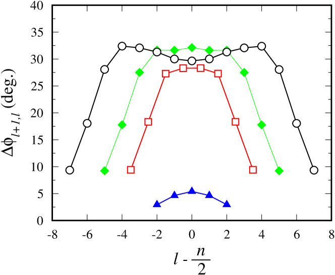
Figure 3: (Colors online) Angle $\Delta\phi_{l}=\phi_{l+1}-\phi_{l}$ between magnetic moments in NN layers $(l+1,l)$ at $T=10$ K, and $L=80$, for representative thicknesses: $n=16$ (black circle), $n=12$ (green diamond), $n=9$ (red square), and $n=6$ (blue up-triangle). Error bars included in the point dimensions.

As emphasized in the the inset of Fig. 2b the magnetizations of NN planes close to the surfaces form angles well lower than those observed in the bulk, an expected consequence of the increasing lack of interactions on one side of the planes as the surface is approached. Such effect can be better looked at by defining the magnetization rotation angle between NN planes $\Delta\phi_{l}\equiv\phi_{l+1}-\phi_{l}$. In Fig. 3 $\Delta\phi_{l}$ is displayed for some representative values of the thickness: for thick samples, surface effects are especially strong only on the first three layers on each film side, and this explains why while for $n\gtrsim 9$ an almost bulk behaviour can be observed, at least for some inner planes, the scenario changes significantly when $n$ drops below 9 (Fig. 2f-h).

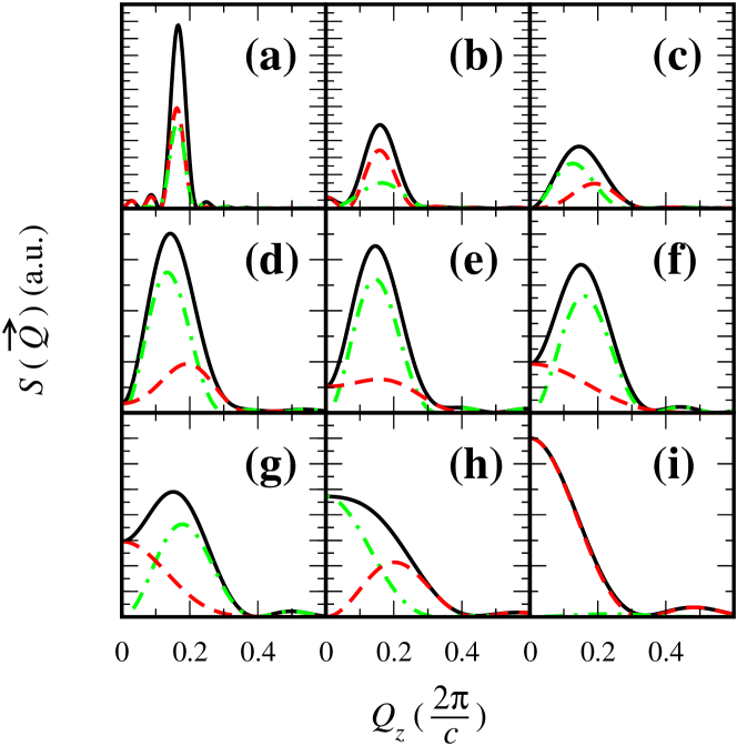
Figure 4: (Colors online) Structure factor $S(0,0,Q_{z})$ (continuous line) vs. $Q_{z}$ at $T=10$ K and layer dimensions $L_{x,y}=80$ for different film thicknesses: (a) $n=36$; (b) $n=16$; (c) $n=12$; (d) $n=11$; (e) $n=10$; (f) $n=9$; (g) $n=8$; (h) $n=7$; (i) $n=6$. Red dashed lines and green dot-dashed lines are the structure factor components along the $x$ or $y$ spin space directions, see text. $Q_{z}$ is measured in reciprocal lattice units $2\pi/c$

.

The characterization of the magnetic order can be further pursued by looking at the static structure factor $S(\vec{Q})$ (where $\vec{Q}=(0,0,Q_{z})$), i.e. to the Fourier transform of the spin correlation function along the $z$-direction of the films. $S(\vec{Q})$ is reported in Fig. 4 (continuous line), together with its in-plane components $S^{xx}(\vec{Q})$ and $S^{yy}(\vec{Q})$ (red and green line, respectively; $x$ and $y$ directions do not obviously have any special meaning and can be chosen at will: here we use the same orientation already employed in Fig. 2). Once again, for $n\gtrsim 11$ (Figs. 4a-d) both the global structure factor and its components shows a clear peak at $Q_{z}^{max}\simeq 0.17$, a value in total agreement with the bulk one $Q_{z}^{bulk}\simeq 1/6$. On the contrary, for $n\leqslant 10$ a fan-like structure appears, signalled by the emergence of an FM component (i.e. a maximum at $Q_{z}=0$) in $S^{xx}(\vec{Q})$ or $S^{yy}(\vec{Q})$ (Fig. 4f-h), while for $n\lesssim 7$ a quasi-collinear spin arrangement is finally reached, as testified by the single maximum of $S(\vec{Q})$ itself at $Q_{z}^{max}=0$ (Fig. 4i).

The results discussed so far show that, at low temperature, the progressive film thickness reduction does not seem to lead to a sudden helical order suppression, but rather to induce a gradual passage to a fan-like order associated with a helix distortion due to the surface effects, until a permanent collapse to an almost collinear order occurs for $n\lesssim 7$. Summing up we can roughly assume that MCS data show that for thickness $n<9$ the helical order is substantially absent.

Such results can be considered in fairly agreement with the experimental outcomes: In fact, in Ref. Weschke04, the authors identified the thickness $n_{0}\simeq 10$ ML as the value indicating the complete lack of helical order, and a thickness uncertainty around about 2 MLcomm must be taken into account.

V Magnetic structures in the order-disorder boundary region

V.1 Layer’s Magnetic Behaviour

This subsection is devoted to the investigation of single layer critical properties for some $n$ values. At the beginning, our attention will be focused on thicknesses close to the Ho helix pitch (12 ML). For this purpose, the order parameter for each spin layer, as defined in Eq. (7), is evaluated, together with its Binder cumulant, Eq. (13), and its susceptibility,Eq. (9). Hereafter, we will denote with the symbol $T_{C,n}$($l$) the transition temperature of the $l-$th layer of the film of thickness $n$.

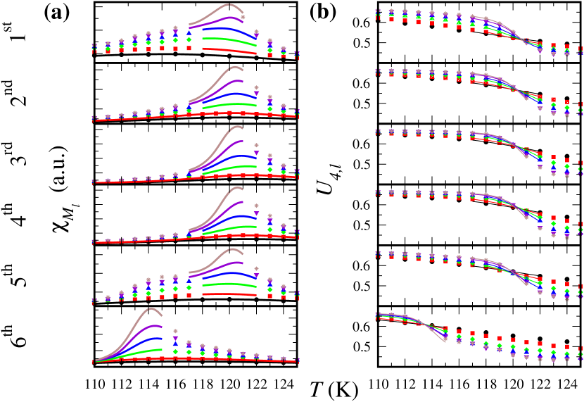
Figure 5: (color online) Susceptibility (a), and Binder cumulant (b) vs. temperature, of the order parameter $M_{l}$ for thickness $n=12$ and $L=12$ (black circle), 16 (red square), 24 (green diamond), 32 (blue up-triangle), 40 (purple down-triangle), and 48 (brown star). $l$ runs from the first to the sixth spin layer. Close to the critical temperature $T_{C,12}$($l$), the continuum lines are obtained by multiple histogram technique.

Susceptibility and Binder cumulant for the first six layers are plotted in Fig. 5 as a function of temperature for different values of lateral dimension $L$ at $n=12$. A critical region in a wide temperature range around $T\sim 120$ K is observed in Fig. 5a for all planes but the central ones (the 6${}^{\textnormal{th}}$ and, for symmetry reason, the 7${}^{\textnormal{th}}$) which are definitely still in a paramagnetic state, displaying instead a critical region shifted around $T\sim 114$ K. Using the Binder cumulant, Eq. (13), for different values of $L$ we can estimate the single layer transition temperature $T_{C,12}(6)=113.4(4)$ K of the inner planes and $T_{C,12}(1\ldots 5)=120.3(4)$ K of the external ones.

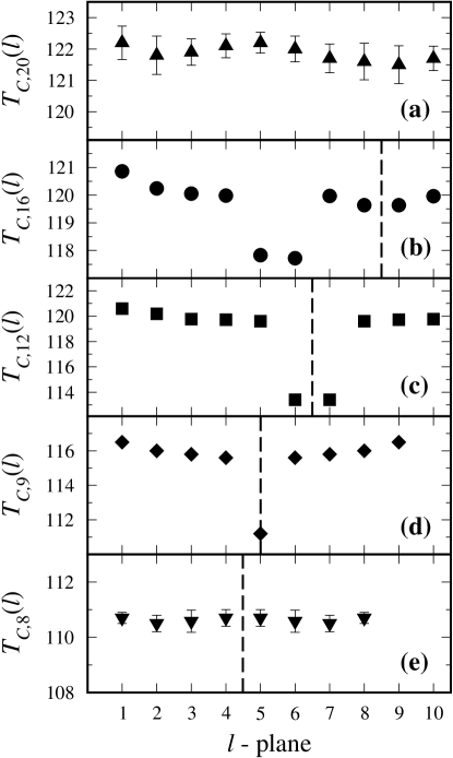
Figure 6: $T_{C,n}$($l$) vs. layer index $l$ for $n=20$ (a), 16 (b), 12 (c), 9(d), and 8(e). The vertical dashed lines denote the position of the bisecting plane of the film, beyond which single-layer properties repeat by symmetry.

The intriguing landscape here observed for $n=12$ is present in the whole range $9\leq n\lesssim 16$. A summarizing picture of the single layer critical temperature $T_{C,n}$($l$) vs. plane index $l$ for $n=$ 20, 16, 12, 9 and 8 is given in Fig. 6: For the thicker film here analyzed ($n=20$, Fig. 6a) $T_{C,20}$($l$) is the same for every layer, and coincides with the establishing of HM order in the film, as expected for the bulk system, where the critical temperature can be obtained both through the chirality, Eq. (6), and by Eq. (8). For $n=16$ (Fig. 6b) we observe a structure more complex than that we find in the films with $n=12$ and $n=9$ (Figs. 6c and Fig. 6d respectively). Indeed, as discussed in details in Ref. Cinti1, , the 5${}^{\textnormal{th}}$, and 6${}^{\textnormal{th}}$ (and, by symmetry, the 11${}^{\textnormal{th}}$ and 12${}^{\textnormal{th}}$) planes lose their order at a lower temperature, $T_{C,16}(5,6,11,12)=117.8(2)$ K, than the others, where $T_{C,16}(1\ldots 4,7\ldots 10,13\ldots 16)=120.1(4)$ K.

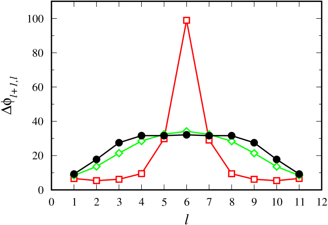
Figure 7: (color online) Angle formed by the magnetization vectors of NN planes, for $n=12$ and $L=48$ at different temperature: $T=10$ K (solid black circle), $T=110$ K (open green diamond), and $T=118$ K (open red square)note2 . Error bars lye within point size.

In order to better understand the magnetic structure in these temperature ranges, we examine the $T$-dependence of the magnetization rotation angle $\Delta\phi_{l}$. For the sake of clarity in Fig. 7 the system $n=12$ is again analyzed. When $T_{C,12}(6)<T<T_{C,12}(1\ldots 5)$ (see, e.g., red square and line in Fig. 7) the ordered layers distinctly display a block structure where $\Delta\phi_{l}$ among the first (last) five planes is almost zero, i.e. $\lesssim 10^{\circ}$; at the same time the angle formed by the magnetization of the two blocks is about $180^{\circ}$note2 . Only for $T<T_{C,12}(6)$ (black and green symbols and lines in Fig. 7), the function $\Delta\phi_{l}$ displays the expected thin films helimagnetic behaviour discussed in Sec.IV (for comparison, see Fig. 5a of Ref. Weschke04, , where the same quantity at $T=0$ is discussed within MFA).

We can graphically represent the block magnetization arrangement for $n=12$ as $\uparrow\uparrow\uparrow\uparrow\uparrow\circ\circ\downarrow\downarrow\downarrow\downarrow\downarrow$, where the circle represents the disordered planes, and the arrows the ordered ones. As above anticipated, the spin block phase is obtained down to $n=9$ (Fig. 6d), where we get an arrangement $\uparrow\uparrow\uparrow\uparrow\circ\downarrow\downarrow\downarrow\downarrow$, and up to $n=16$ (Fig. 6b) where a much more intricate layout, i.e. $\uparrow\uparrow\uparrow\uparrow\circ\circ\downarrow\downarrow\downarrow\downarrow\circ\circ\uparrow\uparrow\uparrow\uparrow$, is observed. It is worthwhile to observe that the AFM alignment of consecutive ordered blocks reveals as the medium range alternating inter-layer exchange coupling give rise to an effective AFM interaction between blocks.

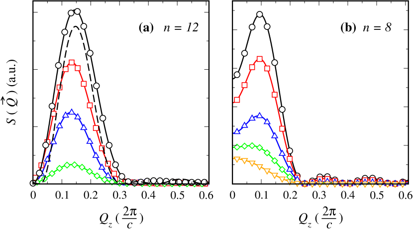
Figure 8: (color online) Temperature evolution of $S(0,0,Q_{z})$ vs. $Q_{z}$. (a): thickness $n=12$ and $L=48$ at $T=10$ K (black line and circle), 113 K (red line and square), 116 K (blue line and triangle), and 121 K (green line and diamond). Dashed black line: $S(\vec{Q})$ of the saturated block structure $\uparrow\uparrow\uparrow\uparrow\uparrow\circ\circ\downarrow\downarrow\downarrow\downarrow\downarrow$. Both the black curve ($T=10$ K) and the dashed one have been divided by a factor equal to ten. (b): thickness $n=8$ and $L=48$ at $T=10$ K (black line and circle), 50 K (red line and square), 90 K (blue line and up-triangle), 105 K (green line and diamond), and 110 K (orange line and down-triangle); all temperatures are lower than $T_{C,8}(1\ldots 8)$.

A further insight in these block phases, especially relevant from an experimental point of view, is obtained by analyzing the behaviour of the structure factor close to $T_{C,n}$($l$). In Fig. 8a $S(\vec{Q})$ for $n=12$ in a wide temperature range is plotted. In particular, one temperature value just below $T_{C,12}(6)$ ($T=113$ K, red line and square), one in the block phase region $T_{C,12}(6)<T<T_{C,12}(1\ldots 5)$ ($T=116$ K, blue line and up-triangle), and one just above $T_{C,12}(1\ldots 5)$ ($T=121$ K, green line and diamonds) have been chosen. As already observed in Sec. II, the prominent broadening in the whole temperature range of the peaks displayed by $S(\vec{Q})$ is mainly a consequence of the intrinsic finite size nature of the films. Excluding an obvious intensity reduction for increasing temperature, one can immediately observe that both shape and peak position are almost unchanged moving from block phases (e.g., $T=116$ K data) to HM order (e.g., $T=113$ K data). A further confirmation of the last statement can be achieved by the comparison, again proposed in Fig. 8a, between the Monte Carlo outcome for $S(\vec{Q})$ at $T=10$ K (black line and circle) and the Fourier transform of the static block structure $\uparrow\uparrow\uparrow\uparrow\uparrow\circ\circ\downarrow\downarrow\downarrow\downarrow\downarrow$ with saturated magnetization for each ferromagnetic plane (black dashed line). As formerly observed for the ultra-thin film $n=16$ Cinti1 , even for $n=12$ the two plots have the same peak position and width; moreover they have comparable intensities too. We are thus led to conclude for the substantial impossibility to distinguish between block phases and helimagnetic order by looking at the structure factor, being it able to give information about the global structure modulation only.

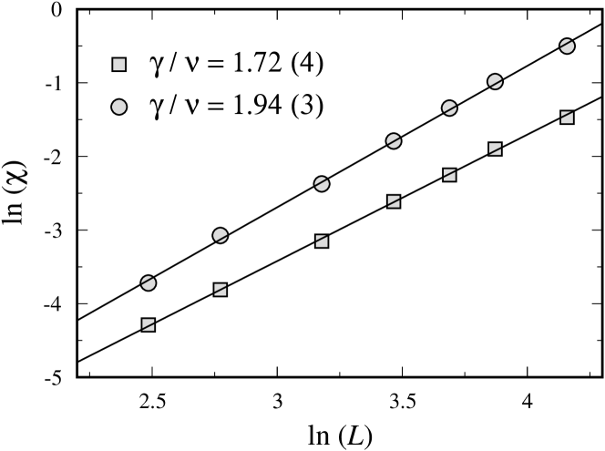
Figure 9: (color online) Logarithm of the susceptibilities $\chi_{M_{5}}$ (square) and $\chi_{M}$ (circle) versus the logarithm of the lateral film dimensions $L$ (error bars included in the symbols), for $n=9$, at $T_{C,9}(5)$ and $T_{C,19}(1\ldots 4,6\ldots 9)$, respectively.

As already observed in Ref. Cinti1, for $n=12$, we find that whenever a blocked phase temperature range occurs, the spins lying on disordered layers are seen to feel a local magnetic field due to inter-layer interactions much smaller than that acting on spins on the ordered layers, so that they behave as being effectively decoupled from the other ones and display the characteristic features of a two-dimensional magnet. The different effective dimensionality of the critical behaviour of lowest-temperature ordering layers from highest-temperature ordering ones, is illustrated in Fig. 9, where an accurate finite-size scaling analysis of the layer magnetic susceptibility $\chi_{M_{5}}$ and of the global susceptibility $\chi_{M}$, at $T_{C,9}(5)$ at $T_{C,9}(1\ldots 4,6\ldots 9)$, respectively, is reported for $n=9$: making use of the usual scaling relation at the critical temperature $\chi\propto L^{\gamma/\nu}$, where $\gamma$ and $\nu$ are the critical exponents of the susceptibility and correlation length, respectively, the value $\gamma/\nu=1.72$ (4), is obtained from the best fit of $\chi_{M_{5}}$ data, while $\gamma/\nu=1.94$ (3) is the result of the fit of $\chi_{M}$. The former value is completely consistent with the Kosterlitz-Thouless behaviour expected in an isolated two-dimensional, easy-plane magnet, while the latter clearly indicates a planar three-dimensional-like trendJanke93a ; Janke93b for the system made by the planes $1\div 4$ and $6\div 9$.

We now move to discuss the MC results obtained for $n=8$. From Fig. 6e the lack of the ordered-disordered blocks mixed structure at intermediate temperature is apparent, as a transition temperature common to all planes ($T_{C,8}(1\ldots 8)=110.6(2)$ K) is found. In Fig. 8b $S(\vec{Q})$ vs. $Q_{z}$ for different $T$ is shown: Close to $T_{C,8}(1\ldots 8)$, we have $Q_{z}^{max}=0$, signalling the presence of a FM-like collinear structure. Subsequently, as the temperature lowers, and the FM spin arrangement opens towards a more stable fan structure, $S(\vec{Q})$ develops a peak at $Q_{z}^{max}=0.095$, but still with a very strong contribution also at $Q_{z}=0$.

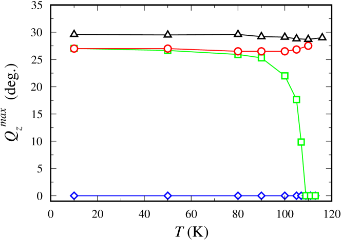
Figure 10: (color online) $Q^{max}_{z}$ vs. temperature for some thicknesses: $n=$ 16 (black line and triangle), 9 (red line and circle), 8 (green line and square), and 7 (blue line and diamond). For $n=8$ the stability of the fan phase with respect to the collinear one is reached only below $T\approx 90$ K (see text).

The evolution of the structure-factor peak position with temperature is better illustrated in Fig. 10, where $Q_{z}^{max}$ vs. $T$ is plotted for some significant values of film thickness. For $n=8$ the clear jump from a collinear structure to a fan-like one (reached at $T\approx 90$ K) is observed: This shows that the onset of order in every plane is by itself not necessarily enough to generate the fan structure observed at low temperature. On the contrary, for thickness values close to the helical pitch and above (where $Q_{z}^{max}$ is essentially independent of temperature) the completion of planes ordering, with the transition of inner layers, marks also the onset of the overall helical/fan arrangement, while for small $n$ a ferromagnetic alignment again stabilizes as soon as the layers simultaneously order. Therefore, the peculiar behaviour of $Q_{z}^{max}(T)$ for $n=8$ can be reasonably attributed to its representing the borderline between helical/block ordered structures and substantially ferromagnetic ones.

In view of the previous discussion, we can conclude that the existence of an intermediate temperature region, characterized by the presence of spin block structures, in between the paramagnetic and the helical ones, seems to be a peculiar feature of non-collinear Ho magnetic films with thickness close enough to the bulk Ho helical pitch; we would like to emphasize that the allowance for at least six inter-layer interactions in the model Hamiltonian (3) turns out to be essential in order to be able to observe such behaviours note .

V.2 Global Film Properties

In this Section we will analyse some macroscopic thermodynamic quantities of the film, and for clarity reasons the attention will be again focused mainly on $n=12$. We will show results pertinent to the magnetic specific heat, the chirality, Eq. (6), and the average order parameter $M$ defined in Eq. (8).

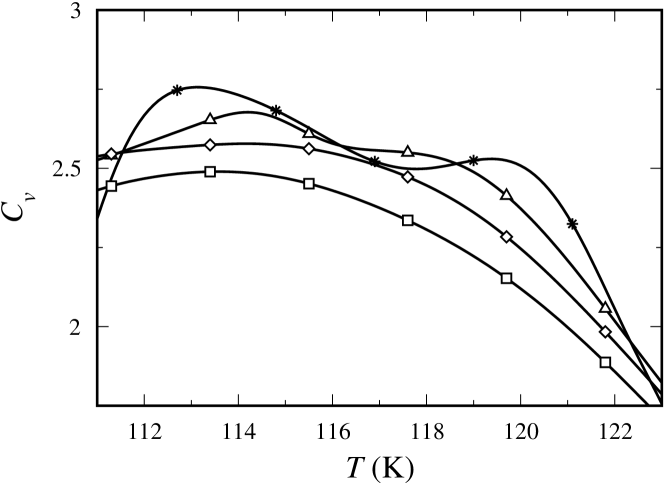
Figure 11: Specific heat $C_{v}$ vs. temperature for thickness $n=12$ and lateral dimension $L=$ 48 (star), 32 (triangle), 24 (diamond), 16 (square).

The first quantity we consider is the specific heat. In Fig. 11, $C_{v}$ at different $L$ is displayed. Its behaviour clearly suggests the presence of two different phase transitions: In fact, two well separated maxima appear in Fig. 11 at $T=113.1$ K and $T=119.4$ K for $L=48$, i.e. close to $T_{C,12}(6)$ and $T_{C,12}(1\ldots 5)$ respectively, making the maxima clear footprints of the block phase regime. Such feature could not be observed in Ref. Cinti1, for $n=16$ film: indeed, the thinner temperature range where the block phase is present, joined with the broad character of the maxima for the finite-size samples investigated, made the two maxima coalesce and impossible to be resolved. Therefore, differently from what happens for $n=12$, in that case the magnetic entropy seems completely released around $T_{C,16}(1\ldots 4,7\ldots 10,13\ldots 16)$.

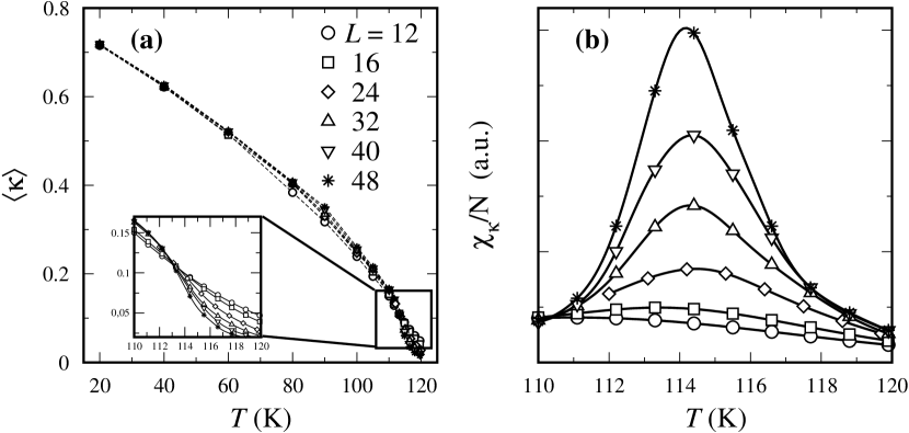
Figure 12: (a) Chirality vs. temperature at $n=12$. The normalization factor is fixed by the bulk factor $\sin Q_{z}^{bulk}$ (see Eq. (6)); error bars are smaller than point size. The continuum lines in the inset are obtained by multiple-histogram algorithm. (b) $\chi_{\kappa}$ obtained by multiple-histogram algorithm. The largest relative error is 0.5% for $L=48$.

The onset of a HM/Fan configuration along the perpendicular film direction can be probed by looking at a related quantity like the chirality, which is plotted in Fig. 12 together with its susceptibility. $\chi_{\kappa}(T)$ does not show any anomaly in the proximity of the highest temperature maximum of $C_{v}$, i.e. around 120 K, while a clear peak appears at $T\simeq 114.2$ K, becoming more and more sharp as $L$ increases.

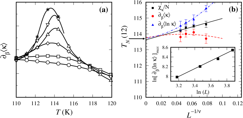
Figure 13: (a): $\partial_{\beta}\langle\kappa\rangle$ vs. temperature for $L=$ 12, 16, 24, 32, 40, 48 (symbols as in Fig. 5). (b): $T_{N}(12)$ plotted vs. $L^{-1/\nu}$ obtained by finite size scaling extrapolation of the three observables, with fitted $\nu$ value. Inset: plot of the maximum value of $\ln\left[\partial_{\beta}\langle\ln\kappa\rangle\right]$ vs. $\ln L$ together with its best fit function (see Eq. (14)).

In order to estimate the transition temperature $T_{N}(12)$, a finite size scaling analysis of the quantities defined in the Eqs. (9), (10), and (11), with $\mathcal{O}=\kappa$, has been carried out. In Fig. 13a $\partial_{\beta}\langle\kappa\rangle$ is reported to show the typical behaviour of such quantities, while Fig. 13b shows details of the fitting and extrapolation procedure. We obtain $\nu$ using it as a free fit parameter in the equation Libbinder ; bunker93 :

$$\partial_{\beta}\ln\kappa\left(t,L\right)=L^{1/\nu}\mathcal{X}\left(tL^{1/\nu}\right)$$ (14)

where $t=\frac{|T-T_{N}(12)|}{T_{N}(12)}$ and $\mathcal{X}$ is an opportune scaling function. At the phase transition $T_{N}(12)$ (i.e. for $t=0$) we can consider the scaling relation (14) as $\left(\partial_{\beta}\ln\kappa\right)_{max}\propto L^{1/\nu}$. Therefore, through an adequate fit, shown in the inset of Fig. 13b, we have obtained $\nu=0.79(2)$. Using such value for $\nu$, we can estimate $T_{N}(12)$ from Eq. (12) by looking at the temperatures where $\langle\chi_{\kappa}\rangle$, $\partial_{\beta}\langle\kappa\rangle$, and $\partial_{\beta}\langle\ln\kappa\rangle$ acquire their maximum value and extrapolating them against $L^{1/\nu}$ as shown in Fig. 13b. The final result obtained is $T_{N}(12)=113.6(1)$ K, a value definitely comparable with $T_{C,12}(6)=113.4(4)$ K: we are thus lead to conclude that the onset of a helical/fan order in the film is only possible when all layers order, so that it is the last ordering spin layer, the 6${}^{\textnormal{th}}$ one for $n=12$, that drives the overall film transition to HM order.

An issue largely debated in literature Diep94 ; Loison00b ; Diepold ; Spanu concerns the order of the chiral transition: In our MCS, in the whole thickness range here analyzed, we did not observe any double-peaked structure in the equilibrium energy distribution at $T_{N}(n)$, i.e., no explicit indication for a first order phase transition is given by our investigation. Anyway a first order transition can not be completely excluded, as suggested in Ref. Loison00b, , where the author reasonably observes that a firm evidence for a first order transition can be obtained only when the sample is much larger than the largest correlation length Loison00b .

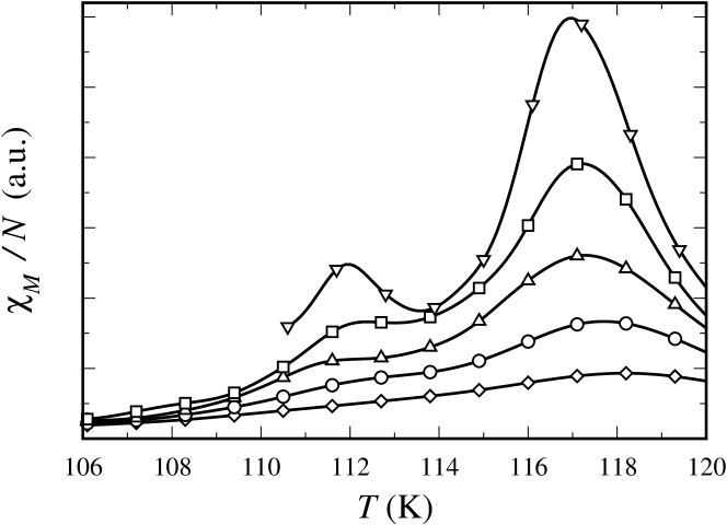
Figure 14: Susceptibility $\chi_{M}$ at $n=9$ and lateral dimensions $L=24$ (diamond), 32 (circle), 40 (up-triangle), 48 (square), and 60 (down-triangle)

The average order parameter $M$ defined in Eq. (8) turns out to probe the physical properties of the system in a way more similar to what is done by the specific heat than by $\kappa$, bearing it signatures of the onset of both spin block and HM/Fan phases, as it is apparent by looking at the related quantity $\chi_{M}$. As an example, $\chi_{M}$ at $n=9$ is reported in Fig. 14: two anomalies are present at $T\simeq 112.0$ K and $T\simeq 117.0$ K, i.e. at temperatures roughly corresponding to $T_{N}(9)=111.2(5)$ K and $T_{C,9}(1\ldots 4)=115.9(4)$ K. We may observe that while the qualitative behaviour of $\chi_{M}$ is similar to that of the specific heat, the peaks in $\chi_{M}$ are sharper and display the finite size scaling typical of a critical quantity, thus making it a better probe to locate transition temperatures.

As the film thickness decreases, the chirality and its related observables display a behaviour similar to that at $n=12$ up to $n=9$, despite a shift from HM to fan-like order (see Fig. 4f); a largely different qualitative behaviour is instead obtained for $n\leq 8$, as already discussed in Sec. V.1.

VI Discussion and Conclusion

In this paper the magnetic properties of thin Ho films have been carefully investigated by extensive MCS, assuming the model pertinent to bulk structure. Regarding the magnetic order below $T_{N}(n)$, it has been showed as, by decreasing the number $n$ of spin layers building the film, a progressive rearrangement of layer’s magnetization from a helical to a fan-like structure (i.e. $S^{xx}(\vec{Q})\neq S^{yy}(\vec{Q})$), and finally to an essentially FM order for $n\leq 7$, is observed. Moreover, for film thickness $n=8$ the structure factor analysis has clearly revealed that once a finite magnetization has been established in every layer, an FM layer arrangement firstly appears which transforms to a fan-like configuration as the temperature is further reduced, as shown in Fig. 10.

Above all that, the system presents very interesting properties around the critical region when the film thickness is comparable with the bulk holmium helical pitch, i.e. for $9\leq n\lesssim 16$. A spin block phase regime is observed in a wide range of intermediate temperatures. In this window some inner planes ($n=16$ has a more complex block structure, as discussed in Ref. Cinti1, ) are in a paramagnetic configuration, while the other ones, close to the surfaces, appear to be in a quasi-FM ordered state (for example, when $n=12$ we have obtained a spin block configuration where the magnetization rotate of an angle $\Delta\phi_{l}\sim 10^{\circ}$ when moving from one spin layer to a neighbouring one within the same block, Fig. 7). Everytime a spin block configuration appears, neighbouring ordered blocks line up in an antiferromagnetic way. What’s more, also the study of macroscopic thermodynamic quantities, as the total energy, the order parameter defined in Eq. (7) and their derivatives, confirms the presence of such large critical regions.

It is worth to remark that making use of all the six inter-layer coupling constants experimentally deduced by Bohr et al. in Ref. Borh89, , it is seen that the competition among surface effects and frustrated inter-layer interactions do not entail a simple adjustment of the surface planes only, but the magnetic critical properties of the whole film are strongly modified as well. Moreover, the results here presented, while confirming that most of the predictions of the MFA employed by Jensen and Bennemann in Ref. Jensen05, are qualitatively correct, also show unambiguously that the thermal fluctuations play an essential role, so that the ability to include their effects is extremely important in order to have a full comprehension of the block phase phenomenology in these films.

A detailed study of the chiraliy, Eq. (6), has shown that $\kappa$ correctly describes the establishing of a global helical/fan order at $T_{N}(n)$ for $n\geq 9$, but such quantity does not result critical in the temperature region where the spin block phase structure appears. Such behaviour of $\kappa$ is also observed in the borderline case $n=8$, where $\kappa$ does not present any anomaly at the single-layer ordering temperature $T_{C,8}(1\dots 8)$.

Another important issue of non-collinear film structures is the impossibility to describe $T_{N}(n)$ vs. $n$ through a well established scaling relation. In fact, as discussed in the Introduction, making use of the empirical relation (1) one can easily only locate the thickness $n_{0}$ which signalizes the disappearance of the HM order. From our results we can reasonably estimate $n_{0}=7\div 9$: The partial disagreement with the experimental results Weschke04 ($n_{0}\approx 10$) could be a consequence both of defects and of the uncertainty with which the thickness of the Ho film experimental samples is known comm .

Finally, a possible comparison between the MCS results and the experimental data Weschke04 ; Weschke05 would require particular care, in order to avoid naïve considerations. Concerning the identification of the magnetic order type, we have shown Cinti1 that the static structure factor alone is not able to distinguish between helical and spin block order. At the same time we think that the characterization of such spin block phases in non-collinear magnetic thin films could be very useful for experimental future works, being the coupling constants strongly dependent both on the used deposition substrate and on the employed deposition technique comm ; sper1 .

- (1) M. E. Fisher and M. N. Barber, Phys. Rev. Lett. 28, 1516 (1972).
- (2) D. S. Ritchie, and M. E. Fisher, Phys. Rev. B 7, 480 (1973).
- (3) M. N. Barber, in Phase Transition and Critical Phenomena, edited by C. Domb and J. Lebowitz (Academic, New York, 1983), Vol.8, Chap. 2.
- (4) M. Henkel, Conformal Invariance and Critical Phenomena (Springer, 1999).
- (5) M. Henkel, et al., Phys. Rev. Lett. 80, 4783 (1998), and references therein.
- (6) R. Zhang and R. F. Willis, Phys. Rev. Lett. 86, 2665 (2001), and references therein.
- (7) P. J. Jensen, and A. R. Mackintosh, Rare Earth Magnetism (Structure and Excitations) (Clarendon Press, Oxford, 1991).
- (8) S. W. Cheong and M. Mostovoy, Nature Materials (London) 6, 13 (2007).
- (9) S. Ishiwata et al., Science 319, 1643 (2008).
- (10) M. Fiebig, J. Phys. D 38, R123 (2005).
- (11) C. Pfleiderer et al., Nature (London) 414, 427 (2001), Nature (London) 427, 227 (2004).
- (12) P. Pedrazzini et al., Phys. Rev. Lett. 98, 047204 (2007).
- (13) P. J. Jensen, and K. H. Bennemann, Surface Science Reports 61, 129 (2006).
- (14) Ultrathin Magnetic Structures, edited by J. A. C. Bland, and B. Heinrich (Springer, New York, 1994).
- (15) E. Weschke et al., Phys. Rev. Lett. 93, 157204 (2004).
- (16) E. Weschke et al., Physica B 357, 16 (2005).
- (17) C. Schüßler-Langeheine et al., Journal of Electron Spectroscopy and Related Phenomena 114-116, 953 (2001); Phys. Rev. Lett. 84, 5624 (2000).
- (18) E. E. Fullerton et al., Phys. Rev. Lett. 75, 330 (1995).
- (19) F. Cinti, A. Cuccoli, and A. Rettori, Phys. Rew. B 78, 020402(R) 2008.
- (20) J. Bohr et al., Physica B 159, 93 (1989).
- (21) D. Gibbs et al., Phys. Rev. Lett. 55, 234 (1985).
- (22) C. C. Larsen, J. Jensen, and A. R. Mackintosh, Phys. Rev. Lett. 59, 712 (1987).
- (23) B. Coqblin, The Electronic Structure of Rare-Earth metal and Alloys (Academic press, 1977).
- (24) H. Zabel (private communicatio).
- (25) T. Moriya, Phys. Rev. 120, 91 (1960).
- (26) I. A. Sergienko, and E. Dagotto, Phys. Rev. B 73, 094434 (2006).
- (27) M. Mostovoy, Phys. Rev. Lett. 96, 067601 (2006).
- (28) S. V. Grigoriev, Yu. O. Chetverikov, D. Lott, and A. Schreyer, Phys. Rev. Lett. 100, 197203 (2008).
- (29) N. Metropolis et al., J. Chem. Phys. 21, 1087 (1953).
- (30) F. R. Brown, and T. J. Woch, Phys. Rev. Lett., 58, 2394 (1987).
- (31) M. E. J. Newman, and G. T. Barkema, Monte Carlo Methods in Statistical Physics (Clarendon Press, Oxford 1999).
- (32) A. M. Ferrenberg, and R. H. Swendsen, Phys. Rev. Lett. 61, 2635 (1988), Phys. Rev. Lett. 63, 1195 (1989).
- (33) A. M. Ferrenberg, D. P. Landau, and R. H. Swendsen, Phys. Rev. E 51, 5092 (1995).
- (34) M. E. J. Newman, and R. G. Palmer, J. Stat. Phys. 97, 1011 (1999).
- (35) H. Kawamura, J. Phys.: Cond. Matt. 10, 4707 (1998).
- (36) See e.g. D. R. Nelson, in Phase Transion and Critical Phenomena, edited by C. Domb and J. Lebowitz (Academic, New York, 1983), Vol.7, Chap. 1, and references therein.
- (37) C. Holm, and W. Janke, Phys. Rev. B 48, 936 (1993).
- (38) W. Janke, and K. Nather, Phys. Rev. B 48, 15807 (1993).
- (39) K. Binder, and J. S. Wang, J. Stat. Phys. 55, 89 (1989).
- (40) A. Bunker, B. D. Gaulin, and C. Kallin, Phys. Rev. B 48, 15861 (1993), Phys. Rev. B 52, 1415 (1995).
- (41) Magnetic Systems with Competing Interactions, edited by H. T. Diep (World Scientific, 1994).
- (42) F. Cinti et al., Phys. Rev. Lett. 100, 057203 (2008), and references therein.
- (43) D. Loison, and P. Simon, Phys. Rev. B 61, 6114 (2000).
- (44) D. Loison, Physica A 275, 207 (2000).
- (45) D. P. Landau, and K. Binder, A Guide to Monte Carlo Simulation in Statistical Physics (Cambridge University Press, Cambridge, 2000).
- (46) K. Binder, Z. Phys. B 43, 119 (1981).
- (47) K. Binder, Phys. Rev. Lett. 47, 693 (1981).
- (48) Bearing in mind the Binder cumulant analysis of Fig. 5, at K are really meaningless, because the 6 and 7 layer still are in a substantially paramagnetic state; the relative points in Fig. 7 (red square and line) are reported for continuity, and only the sum is to be considered physically sound.
- (49) In a model Hamiltonian where two inter-layer coupling constant only ( and along the -directions) are taken into account, a substantially different behaviour is observed: this topic will be more detailly addressed and discussed in a forthcoming paper.
- (50) H. T. Diep, Phys. Rev. B 39, 397 (1989).
- (51) R. Quartu, and H. T. Diep, Journal of Magnetism and Magnetic Materials 182, 38 (1998).
- (52) J. Kwo, in Thin Film Techniques for Low-Dimensional Structure, edited by R. F. C. Farrow, S. S. P. Parkin, P. J. Dobson, N. H. Neaves, and A. S. Arrott (Plenum, New York, 1988) NATO ASI Ser. B Vol. 13.