Ph.D. Thesis

Anisotropic Ground States of the Quantum Hall System
with Currents

Abstract

Anisotropic states at half-filled third and higher Landau levels are investigated in the system with a finite electric current. We study the response of the striped Hall state and the anisotropic charge density wave (ACDW) state against the injected current using the effective action. Current distributions and a current dependence of the total energy are determined for both states. With no injected current, the energy of the ACDW state is lower than that of the striped Hall state. We find that the energy of the ACDW state increases faster than that of the striped Hall state as the injected current increases. Hence, the striped Hall state becomes the lower energy state when the current exceeds the critical value. The critical value is estimated at about $0.04$ - $0.05$ nA, which is much smaller than the current used in the experiments.

Contents

1. Acknowledgment
2. Abstract
3. 1 Introduction
4. 2 Review of the von Neumann lattice formalism
   1. 2.1 Orthonormal von Neumann lattice basis
      1. 2.1.1 Landau level quantization
      2. 2.1.2 Eigenstate of the magnetic angular momentum operator
      3. 2.1.3 Coherent state
   2. 2.2 Magnetic translation group and von Neumann Lattice basis
      1. 2.2.1 Magnetic translation group
      2. 2.2.2 Eigenstate of the commutative magnetic translation operators
   3. 2.3 von Neumann lattice formalism
      1. 2.3.1 Hamiltonian of the quantum Hall system
      2. 2.3.2 Hartree-Fock Hamiltonian
      3. 2.3.3 Density operator
      4. 2.3.4 Magnetic field in momentum space
5. 3 Periodic states in the quantum Hall system
   1. 3.1 Background
      1. 3.1.1 Early studies
      2. 3.1.2 vNL formalism for striped Hall, CDW, and bubble states
   2. 3.2 Striped Hall state
      1. 3.2.1 Assumption of the unidirectional density
      2. 3.2.2 Diagonalization, eigenstates and eigenvalues
      3. 3.2.3 Self-consistency condition and solution
   3. 3.3 Charge density wave state
      1. 3.3.1 Assumption of the CDW density
      2. 3.3.2 Diagonalization, eigenstates and eigenvalues
      3. 3.3.3 Self-consistency condition
      4. 3.3.4 Density profile and Energy dispersion of CDW states
   4. 3.4 Bubble state
      1. 3.4.1 Assumption of the bubble density
      2. 3.4.2 Self-consistency condition and solution
      3. 3.4.3 Relation between the $N$-electron bubble state and the CDW state at $\nu^{\ast}=1/M$
6. 4 Effects of an injected current on highly anisotropic states
   1. 4.1 Introduction
   2. 4.2 Experiments of highly anisotropic states
   3. 4.3 Highly anisotropic states in the Hartree-Fock theory
      1. 4.3.1 Striped Hall state at $\nu^{\ast}=1/2$
      2. 4.3.2 Anisotropic charge density wave state at $\nu^{\ast}=1/2$
   4. 4.4 Response functions
      1. 4.4.1 Response function of the striped Hall state
      2. 4.4.2 Response function of the anisotropic charge density wave state
   5. 4.5 Energy corrections due to injected currents
      1. 4.5.1 Current and charge distributions
      2. 4.5.2 Energy corrections
   6. 4.6 Summary
7. A von Neumann lattice formalism
   1. A.1 Wave function of the von Neumann lattice basis
   2. A.2 Explicit form of the inner product $\langle\alpha_{\bf p}|\alpha_{{\bf p}^{\prime}}\rangle$
   3. A.3 Density operator on the von Neumann lattice basis
   4. A.4 Landau level matrix elements
   5. A.5 Hartree-Fock Hamiltonian
      1. A.5.1 Hartree term
      2. A.5.2 Fock term
8. B Highly anisotropic states
   1. B.1 Deviation of the Hartree-Fock Hamiltonian due to currents
   2. B.2 Calculation of $K^{00}$ for the ACDW state

Chapter 1 Introduction

Since the discovery of the integer quantum Hall effect by von Klitzing et al. [1] in 1980, a two-dimensional (2D) electron system in a perpendicular magnetic field has attracted much attention for more than a quarter of a century. In 1980, von Klizing et al. have measured the Hall conductivity of the 2D electron system in strong perpendicular magnetic fields at low temperatures, and have found that the Hall conductivity exhibits plateaus just at integer multiples of $e^{2}/h$ as the magnitude of the magnetic field is varied, where $e(>0)$ is the electron charge and $h$ is the Plank constant. This is the integer quantum Hall effect (IQHE), and after its discovery, a 2D electron system subjected to a perpendicular magnetic field is called a quantum Hall system. The integer quantization of the Hall conductivity is closely related to a Landau level quantization of an energy spectrum of free electrons as follows. In classical mechanics, a free electron performs a cyclotron motion in a uniform magnetic field $B$. Since this cyclotron motion corresponds to a harmonic oscillation with the cyclotron frequency $\omega_{c}=eB/m_{e}$ ($m_{e}$: electron mass) in quantum mechanics, the energy spectrum is quantized to $E_{l}=\hbar\omega_{c}(l+1/2)$ ($l=0,1,2,\dots$). This quantized energy level is called Landau level (LL) named after Landau who solved this problem for the first time. The number of states in each LL is proportional to $B$, and when the magnetic field is strong and the lower few LLs are fully occupied by electrons, the Hall conductivity is quantized. Thus, the IQHE is closely related to the LL quantization. In order to explain the emergency of the plateau structure, a localization effect of electrons trapped by impurities should be taken into account and this provides another interesting topic. For more details about the IQHE, see the reviews by Ando et al. [2] and Störmer [3].

Only two years later after the discovery of the IQHE, another surprising phenomenon, a fractional quantum Hall effect (FQHE), was found. In 1982, working with much higher mobility sample, Tsui et al. [4] have discovered the fractional quantization of the Hall conductivity. The fractional quantizations have been observed around characteristic partial fillings in the lowest LL. Around these fillings, electron-electron interaction plays a predominant role, which results in a unique collective phenomenon. Among a number of theoretical studies done to solve this problem, it was Laughlin [5] who has succeeded in discovering a Laughlin’s variational wave function which explains the fractional quantization at the characteristic fillings. The fact that the Laughlin wave function is a good variational wave function implies that the ground state at these fillings is a translationally invariant liquid state. Now, various studies support this conclusion. After the discovery of the Laughlin’s wave function, his novel work has evolved into a concept of a composite Fermion which is an electron bound to an integer number of magnetic flux quanta. Composite Fermion is based on the observation by Jain [6] that the Laughlin’s wave function could be viewed as integer quantum Hall states of composite Fermions with an even number of flux quanta, in a very natural way. On the basis of this prominent idea, most experimental results for the FQHE can be explained naturally, which supports the idea of the composite particles experimentally. The composite Fermion has provided exciting fields of theoretical studies since its discovery by Jain. For more details, see the reviews by Jain and Kamilla [7].

There are many interesting topics other than the IQHE and the FQHE, especially in higher LLs where various electron solid phases exist. In 1996, Koulakov et al. [8] have studied a possibility of charge density wave (CDW) states in higher LLs, which include bubble states (CDW states with two or more electrons per unit cell) and striped Hall states (unidirectional charge density wave states), within the Hartree-Fock (HF) theory. They have found that CDW and bubble states are energetically favorable in higher LLs, and in particular around half fillings, striped Hall states are energetically favorable. Indeed, in 1999, working with ultra-high mobility samples at low temperatures, Lilly et al. [9] and Du et al. [10] have reported the highly anisotropy in the longitudinal resistivity, which is interpreted as due to a formation of stripe states or anisotropic charge density wave (ACDW) states. Away from half-fillings, more precisely around $\nu=4+1/4$, $4+3/4$, reentrant integral quantizations of the Hall conductivity have been observed [10, 11]. This reentrant integer quantum Hall effect (RIQHE) is interpreted as due to a collective insulating property of a bubble state pinned by impurities. Although these intriguing phenomena in higher LLs have been studied intensively over ten years, many issues still remain to be solved. Among them, we focus on the highly anisotropic states. While experimental features of the anisotropic states suggest that the anisotropic states are the striped Hall states, the ACDW state has a slightly lower energy than the striped Hall state within the HF theory with no electric current. This has been an enigma as to the anisotropic states. In experiments of the anisotropic states, current is injected. This effect has not been taken into account in the previous calculations. We focus on this fact and investigate the effect of the injected current on the striped Hall states and the ACDW states by calculating response functions against the injected current [12]. This is one of main topics of this thesis. The details are given in Chapter 4.

Another main topic of this thesis is a calculational method for periodic states in the quantum Hall system by means of a von Neumann lattice (vNL) basis [13, 14]. Most theoretical studies of the quantum Hall system start by expansion of the Hamiltonian using a complete set of eigenstates of free electrons in a magnetic field. There are mainly three different complete sets to be used according to the purpose:

1. Eigenstates of a magnetic angular momentum operator

2. Eigenstates of a magnetic translation operator in one-direction

3. A complete set of a vNL basis which we use aggressively in this thesis

All of them are closely related to a magnetic flux $\phi_{0}=h/e$, and $\phi_{0}$ is closely related to a magnetic translation group as follows. As has been mentioned, eigenenergies of electrons in a uniform magnetic field $B$ are quantized to LLs and each LL has a large number of degeneracy given by $N_{\phi}=SB/\phi_{0}$, where $S$ is a total area of the 2D system. This number of degeneracy is equal to the number of magnetic flux quanta penetrating the system, which means that one state in each LL occupies an area penetrated by one magnetic flux. This fact can be viewed from a point of view of a magnetic translation. In the case of no magnetic field, translation operators commute with each other and they commute with a free Hamiltonian, too. Therefore, a momentum is well-defined as a good quantum number. On the other hand, in the presence of a uniform magnetic field, previous translation operators are not commutative with the free Hamiltonian anymore. This is because the vector potential generating the magnetic field is not uniform in coordinate space even if a magnetic field is uniform. To obtain the proper translation operator, the previous translation operator should be modified to a magnetic translation operator which is commutative with the free Hamiltonian in the uniform magnetic field. After we obtain the proper translation operators, two linearly independent magnetic translation operators are still non-commutative with each other for an arbitrary translation. Only discrete translation operators are commutative with each other, which span a magnetic translation group [15]. For these discrete operators, a momentum is well-defined as a good quantum number, and the momentum is reduced to a magnetic Brillouin zone owing to the discrete translation symmetry. Actually, the vNL basis is an eigenstate of these discrete magnetic translation operators so that it has a momentum as a good quantum number and periodicities in two linearly independent directions. The area spanned by the two different unit magnetic translation operators is given by $S_{a}=\phi_{0}/B=h/eB$ which corresponds to an area penetrated by $\phi_{0}$. Hence, the area occupied by one electron and a magnetic translation group are closely related to each other.

Three complete sets mentioned above are discretized as one state occupies an area $S_{a}$ as follows:

1. For the complete set of eigenstates of a magnetic angular momentum operator, the eigenstate is characterized by the eigenvalue of a magnetic angular momentum operator $\hbar(l-m)$, where $l$ is the LL index and $m$ is a nonnegative integer. The probability density of the eigenstate with $m$ is localized on the circumference with a radius $r_{m}=\sqrt{m/\pi}\,a$ with $a=\sqrt{h/eB}$, which gives $S_{a}$ per eigenstate.

2. For the complete set of eigenstates of a translation operator in one direction (which is set to $y$), while the probability density in the $y$-direction is uniform, the density in the $x$-direction is localized at discrete coordinates with the interval $\Delta x=\phi_{0}/BL_{y}$, where $L_{y}$ is the system size in the $y$-direction, which gives $S_{a}$ per eigenstate, too.

3. For the complete set of the vNL basis, the probability density is localized at lattice sites with an area of the unit cell given by $S_{a}$, which naturally gives $S_{a}$ per eigenstate.

Thus, all of three basis sets are closely related to $\phi_{0}$ which is closely related to the magnetic translation group. As for the vNL basis, the periodicity of the vNL can be deformed as long as the area of the unit cell is kept to $S_{a}$. From this point of view, we develop the vNL formalism to analyze periodic states, which include striped Hall states, ACDW states, and Bubble states. The vNL basis is the most suitable basis among three sets of basis mentioned above since it can be deformed as the periodicity of the vNL coincides with the periodicity of the periodic state. The details are given in Chapter 3. The study of the highly anisotropic states in this thesis is one of applications of this formalism. There will be some other applications of this formalism to study periodic states in the quantum Hall system, which is one of our future plans.

This thesis is organized as follows. In Chapter 2, a von Neumann lattice formalism is reviewed. Some useful relations and features peculiar to the von Neumann lattice formalism are also reviewed. In Chapter 3, a calculational method by means of the von Neumann lattice formalism is developed to study periodic states in the quantum Hall system. In Chapter 4, effects of an injected current on highly anisotropic states are studied using the von Neumann lattice formalism developed in Chapter 3. Some concrete calculations are presented in Appendixes.

Chapter 2 Review of the von Neumann lattice formalism

In this chapter, we review the von Neumann lattice formalism which is a powerful tool to study periodic states in the quantum Hall system as has been mentioned in the previous chapter. The von Neumann lattice basis is an eigenstate of commutative magnetic translation operators, which spans a Hilbert space in the quantum Hall system in conjunction with a Landau level space. The von Neumann lattice basis is first introduced as a complete set of coherent states. Since they are coherent states, two different states are not orthogonalized. However, by Fourier transforming and normalizing them, we obtain a discrete set of orthonormal von Neumann lattice basis as a complete set of one-particle eigenstates. We review this procedure and show that the obtained basis is indeed the eigenstate of commutative magnetic translation operators. Some useful relations and features peculiar to the von Neumann lattice basis are also reviewed.

Note that in this thesis, we only consider the rectangular von Neumann lattice basis for simplicity. However, the oblique von Neumann lattice can be obtained by a similar procedure. For details, see Ref. [14].

2.1 Orthonormal von Neumann lattice basis

2.1.1 Landau level quantization

Let us consider a two-dimensional (2D) electron system in the $x$-$y$ plane subjected to a perpendicular magnetic field ${\bf B}=(0,0,B)$. In the absence of electron-electron interactions, electrons just perform a cyclotron motion with a cyclotron frequency $\omega_{c}=eB/m_{e}$. Since this cyclotron motion corresponds to a harmonic oscillator in quantum mechanics, one expects that the energy level is quantized to $E_{l}=\hbar\omega_{c}(l+1/2)$ with $l=0,1,2,\dots$. We confirm this quantization by a microscopic analysis below.

The cyclotron motion is represented by a guiding center coordinates ${\bf X}=(X,Y)$ and the relative coordinates ${\bm{\xi}}=(\xi,\eta)$ as

$$x=X+\xi,\quad y=Y+\eta,$$ (2.1)

$$\xi=\frac{1}{eB}(-i\hbar\partial_{y}+eA_{y}),\quad\eta=-\frac{1}{eB}(-i\hbar\partial_{x}+eA_{x}).$$ (2.2)

where ${\bf B}=\nabla\times{\bf A}({\bf x})$ and $e>0$ is the electron charge. Here, ${\bf X}$ and ${\bm{\xi}}$ satisfy the following commutation relations,

$$[X,Y]=-[\xi,\eta]=i\frac{\hbar}{eB},\quad[X,\xi]=[X,\eta]=[Y,\xi]=[Y,\eta]=0.$$ (2.3)

By using these coordinates, the one-particle free Hamiltonian $H_{0}=(-i\hbar\nabla+e{\bf A}({\bf x}))^{2}/2m_{e}$ is expressed by

$$H_{0}=\frac{m_{e}\omega_{c}^{2}}{2}(\xi^{2}+\eta^{2}).$$ (2.4)

Next, we introduce new operators $L_{A},L_{A}^{\dagger},L_{B},L_{B}^{\dagger}$ as

$$L_{A}=-\frac{1}{\sqrt{2}\,l_{B}}(\eta+i\xi),\quad L_{A}^{\dagger}=-\frac{1}{\sqrt{2}\,l_{B}}(\eta-i\xi)$$

$$L_{B}=\frac{1}{\sqrt{2}\,l_{B}}(X+iY),\quad L_{B}^{\dagger}=\frac{1}{\sqrt{2}\,l_{B}}(X-iY),$$ (2.5)

where $l_{B}=\sqrt{\hbar/eB}$ is the magnetic length. Since these operators satisfy the following commutation relations,

$$[L_{A},L_{A}^{\dagger}]=[L_{B},L_{B}^{\dagger}]=1,\quad[L_{A},L_{B}]=[L_{A}^{\dagger},L_{B}^{\dagger}]=[L_{A},L_{B}^{\dagger}]=[L_{A}^{\dagger},L_{B}]=0.$$ (2.6)

new operators can be regarded as independent two kinds of creation and annihilation operators. Using these operators, we rewrite the one-particle free Hamiltonian $H_{0}$ as

$$H_{0}=\hbar\omega_{c}(L_{A}^{\dagger}L_{A}+\frac{1}{2}).$$ (2.7)

This is a Hamiltonian of a harmonic oscillator with a frequency $\omega_{c}$. The eigenstate and eigenvalue of $H_{0}$ are given by

$$|f_{l}\rangle=\frac{(L_{A}^{\dagger})^{l}}{\sqrt{l!}}|f_{0}\rangle,\quad H_{0}|f_{l}\rangle=E_{l}|f_{l}\rangle,$$ (2.8)

where $|f_{0}\rangle$ satisfies $L_{A}|f_{0}\rangle=0$. Hence, the naive expectation with respect to the quantization of the energy level is confirmed. The energy level labeled by $l$, $E_{l}=\hbar\omega_{c}(l+1/2)$, is called the $l$th Landau level (LL).

2.1.2 Eigenstate of the magnetic angular momentum operator

In the above discussion, the guiding center coordinates are not used to derive the LL quantization. Since the free Hamiltonian $H_{0}$ is commutative with the guiding center coordinates, each LL has degeneracy coming from the eigenstate related to the guiding center coordinates. The most simple one is the eigenstate of the operator $L^{\dagger}_{B}L_{B}$. This eigenstate is given by

$$|J_{M}\rangle=\frac{(L^{\dagger}_{B})^{M}}{\sqrt{M!}}|J_{0}\rangle,\quad L^{\dagger}_{B}L_{B}|J_{M}\rangle=M|J_{M}\rangle\quad(M=0,1,2,\dots),$$ (2.9)

where $L_{B}|J_{0}\rangle=0$. The direct product $|f_{l}\rangle\otimes|J_{M}\rangle\equiv|l,M\rangle$ is a simultaneous eigenstate of the free Hamiltonian $H_{0}$ and the operator $J=(eB/2)(\xi^{2}+\eta^{2}-X^{2}-Y^{2})=\hbar(L^{\dagger}_{A}L_{A}-L^{\dagger}_{B}L_{B})$, and spans a Hilbert space of a one-particle state. Actually, the operator $J$ is a magnetic angular momentum operator since it commutes with the free Hamiltonian, and when the magnetic field is set to zero, it takes $J(B=0)=-i\hbar(x\partial_{y}-y\partial_{x})$ which is an angular momentum operator in the absence of a magnetic field. Here, the fact that ${\bf A}({\bf x})$ is proportional to $B$ is used. The electron density of the eigenstate with $M$ is localized on the circumference with a radius $r_{M}=\sqrt{M/\pi}\,a$ with $a=\sqrt{h/eB}$, which gives the area $S_{a}=h/eB=\phi_{0}/B$ ($\phi_{0}=h/e$ is a magnetic flux quantum) per eigenstate as has been mentioned in the previous chapter (see also Appendix A.1). Note that each LL has the degeneracy factor $N_{\phi}=BS/\phi_{0}$ ($S$ is a total area of the 2D system), which means that the number of degeneracy in each LL is equal to the number of magnetic flux quanta penetrating the 2D system.

2.1.3 Coherent state

There is another eigenstate constructed by the guiding center coordinate, that is, a coherent states of the guiding center coordinates,

$$(X+iY)|\alpha_{m,n}\rangle=z_{m,n}|\alpha_{m,n}\rangle,\quad z_{m,n}=a(r_{s}m+i\frac{n}{r_{s}}),$$ (2.10)

where $m$ and $n$ are integers. In coordinate space, these coherent states are localized at the rectangular lattice point $a(mr_{s},n/r_{s})$, where $a=\sqrt{h/eB}$ is a lattice constant, and $r_{s}$ is an asymmetry parameter of the unit cell (see Appendix A.1). The magnitude of $a$ is of the order of tens of nano meter for a few Tesla of magnetic field. Since the number of these coherent states in each Landau level is equal to $N_{\phi}$, the direct product $|f_{l}\rangle\otimes|\alpha_{m,n}\rangle\equiv|l,{\bf N}\rangle$ with ${\bf N}=(m,n)$ forms the complete set of a one-particle state. Note that the completeness of this coherent set is ensured mathematically [16, 17, 18] and this set is called von Neumann lattice (vNL) basis [13, 14].

Since $[L_{B},L_{B}^{\dagger}]=1$, we can take $L_{B}=\partial/\partial L_{B}^{\dagger}$. Thus,

$$L_{B}|\alpha_{m,n}\rangle=\frac{\partial}{\partial L_{B}^{\dagger}}|\alpha_{m,n}\rangle=\frac{z_{m,n}}{\sqrt{2}\,l_{B}}|\alpha_{m,n}\rangle,$$ (2.11)

and $|\alpha_{m,n}\rangle$ is given by

$$|\alpha_{m,n}\rangle=C_{m,n}e^{(z_{m,n}/\sqrt{2}\,l_{B})L_{B}^{\dagger}}|\alpha_{0,0}\rangle,$$ (2.12)

where $C_{m,n}$ is a normalization constant. If we set $\langle\alpha_{m,n}|\alpha_{m,n}\rangle=1$, then $|C_{m,n}|=e^{-\pi|z_{m,n}|^{2}/2a^{2}}$ with an arbitrary phase factor. We use $e^{i\pi(m+n+mn)}$ as a phase factor of $C_{m,n}$ throughout this thesis and set $a=1$ unless otherwise stated.

The eigenstate $|\alpha_{m,n}\rangle$ is not an orthogonal basis since it is a coherent state. However, the inner product,

$$\langle\alpha_{m,n}|\alpha_{m^{\prime},n^{\prime}}\rangle=e^{i\pi\{(m-m^{\prime})+(n-n^{\prime})+(m-m^{\prime})(n-n^{\prime})\}}e^{-(\pi/2)\{(m-m^{\prime})^{2}r_{s}^{2}+(n-n^{\prime})^{2}/r_{s}^{2}\}},$$ (2.13)

is a function of the difference, $(m-m^{\prime})$ and $(n-n^{\prime})$, so that the Fourier representation of $|\alpha_{m,n}\rangle$ becomes an orthogonal basis. Indeed, by using the momentum representation of $|\alpha_{m,n}\rangle$,

$$|\alpha_{\bf p}\rangle=\sum_{m,n}e^{imp_{x}+inp_{y}}|\alpha_{m,n}\rangle,$$ (2.14)

the inner product of $|\alpha_{\bf p}\rangle$ is calculated as (see Appendix A.2)

$$\langle\alpha_{\bf p}|\alpha_{{\bf p}^{\prime}}\rangle=\beta^{\ast}({\bf p})\beta({\bf p}^{\prime})(2\pi)^{2}\sum_{\bf N}\delta^{2}({\bf p}-{\bf p}^{\prime}-2\pi{\bf N})e^{i\phi({\bf p},{\bf N})},$$

$$\beta({\bf p})=(\sqrt{2}\,r_{s})^{1/2}e^{-(r_{s}p_{y})^{2}/4\pi}\theta_{1}\left(\frac{p_{x}+ir_{s}^{2}p_{y}}{2\pi}\Biggm{|}ir_{s}^{2}\right),$$ (2.15)

where $\theta_{1}(v|\tau)=i\sum^{\infty}_{n=-\infty}e^{i\pi n+i\pi\tau(n-1/2)^{2}+i\pi v(2n-1)}$ is a Jacobi’s theta function of the first kind, $\phi({\bf p},{\bf N})=\pi(m+n)-p_{x}n$, and we set $a=1$. Thus, we obtain the orthonormal vNL basis by normalizing $|\alpha_{\bf p}\rangle$ as

$$|\beta_{\bf p}\rangle=\frac{1}{\beta({\bf p})}|\alpha_{\bf p}\rangle.$$ (2.16)

From the property of the theta function, $\beta({\bf p})$ and $|\beta_{\bf p}\rangle$ obeys the following nontrivial boundary condition,

$$\beta({\bf p}+2\pi{\bf N})=e^{i\phi({\bf p},{\bf N})}\beta({\bf p}),\quad|\beta_{{\bf p}+2\pi{\bf N}}\rangle=e^{-i\phi({\bf p},{\bf N})}|\beta_{\bf p}\rangle.$$ (2.17)

Using this boundary condition, we obtain the momentum space reduced to the Brillouin zone (BZ), $-\pi<p_{x},p_{y}<\pi$, hence, the Hilbert space of a one-particle state is spanned by the state $|l,{\bf p}\rangle=|f_{l}\rangle\otimes|\beta_{\bf p}\rangle$. Owing to the boundary condition (2.17), $|\beta_{\bf p}\rangle$ satisfies

$$\langle\beta_{\bf p}|\beta_{{\bf p}^{\prime}}\rangle=(2\pi)^{2}\sum_{\bf N}\delta^{2}({\bf p}-{\bf p}^{\prime}-2\pi{\bf N})e^{i\phi({\bf p},{\bf N})}.$$ (2.18)

The left hand side and the right hand side of Eq. (2.18) obey the same boundary condition. If we restrict the momentum range to the first Brillouin zone, then Eq. (2.18) becomes $\langle\beta_{\bf p}|\beta_{{\bf p}^{\prime}}\rangle=(2\pi)^{2}\delta({\bf p}-{\bf p}^{\prime})$ which expresses a usual orthonormal relation.

2.2 Magnetic translation group and von Neumann Lattice basis

2.2.1 Magnetic translation group

The translation operator in the system with zero magnetic field is given by

$$T({\bm{\delta}})=e^{i{\bm{\delta}}\cdot\hat{\bf p}/\hbar}$$ (2.19)

where $\hat{\bf p}=-i\hbar\nabla$. Indeed, if $T({\bm{\delta}})$ acts on a one-particle wave function $\psi({\bf x})$, then $\psi({\bf x})$ is translated to $\psi({\bf x}+{\bm{\delta}})$. The translation operator $T({\bm{\delta}})$ commutes with the one-particle free Hamiltonian $H_{0}(B=0)=\hat{\bf p}^{2}/2m_{e}$, and $T({\bm{\delta}}_{x})$ and $T({\bm{\delta}}_{y})$ are commutative for an arbitrary $\delta_{x}$ and $\delta_{y}$, where ${\bm{\delta}}_{x}=\delta_{x}\hat{\bf e}_{x}$, ${\bm{\delta}}_{y}=\delta_{y}\hat{\bf e}_{y}$, and $\hat{\bf e}_{x}$ and $\hat{\bf e}_{y}$ are unit vectors in the $x$ and $y$ directions, respectively. Hence, we can take $\{H_{0},T({\bm{\delta}}_{x}),T({\bm{\delta}}_{y})\}$ as a set which can be diagonalized simultaneously. The situation becomes different when a magnetic field is applied. Let us consider the 2D electron system in a uniform magnetic field ${\bf B}=(0,0,B)$. In this case, the one-particle Hamiltonian is given by $H_{0}=(\hat{\bf p}+e{\bf A}({\bf x}))^{2}/2m_{e}$ and the electron performs a cyclotron motion. Clearly, $T({\bm{\delta}})$ does not commute with $H_{0}$ since the vector potential ${\bf A}({\bf x})$ depends on ${\bf x}$ even if the magnetic field is uniform. In order to obtain the proper translation operator, magnetic translation operator, which commutes with $H_{0}$, the gauge transformation which brings ${\bf A}({\bf x}+{\bm{\delta}})$ back to ${\bf A}({\bf x})$ is required in conjunction with $T({\bf\delta})$. This magnetic translation operator is given by

$$\hat{T}({\bm{\delta}})=e^{i{\bm{\delta}}\cdot{\bf K}/\hbar},\quad{\bf K}=\hat{\bf p}+e{\bf A}({\bf x})-e{\bf B}\times{\bf x}.$$ (2.20)

Since ${\bf K}$ is rewritten as ${\bf K}=eB(Y,-X)$ and $H_{0}$ is rewritten as Eq. (2.4), it is clear that $\hat{T}({\bm{\delta}})$ indeed commutes with $H_{0}$.

The magnetic translation operator $\hat{T}({\bm{\delta}})$ includes the spatial translation and the gauge transformation. To make this point clear, we divide $\hat{T}({\bm{\delta}})$ into two parts. Using the Cambell-Hausdorff formula,

$$\exp{A}\exp{B}=\exp(A+B+\frac{1}{2}[A,B]+\frac{1}{12}[A-B,[A,B]]+\dots),$$ (2.21)

we rewrite $\hat{T}({\bm{\delta}})$ as

$$\hat{T}({\bm{\delta}})=e^{i\theta/2}e^{i{\bm{\delta}}\cdot e({\bf A}-{\bf B}\times{\bf x})/\hbar}e^{i{\bm{\delta}}\cdot\hat{\bf p}/\hbar},$$ (2.22)

where $i\theta=[i{\bm{\delta}}\cdot e({\bf A}({\bf x})-{\bf B}\times{\bf x})/\hbar,i{\bm{\delta}}\cdot\hat{\bf p}/\hbar]$ is constant and the vector potential ${\bf A}({\bf x})$ is assumed to be a linear function of x. This expression clearly shows that $\hat{T}(\bm{\delta})$ consists of the spatial translation operator $T({\bm{\delta}})$ and the gauge transformation operator $e^{i\theta/2}e^{i{\bm{\delta}}\cdot e({\bf A}-{\bf B}\times{\bf x})/\hbar}$.

The magnetic translation operators do not commute with each other for arbitrary two translations owing to the non-commutativity of $K_{x}$ and $K_{y}$, i.e., $[K_{x},K_{y}]=i\hbar eB$. For simplicity, we consider two linearly independent magnetic translation operators, $\hat{T}({\bm{\delta}}_{x})=e^{i\delta_{x}K_{x}/\hbar}$ and $\hat{T}({\bm{\delta}}_{y})=e^{i\delta_{y}K_{y}/\hbar}$. Using the commutation relation of $K_{x}$ and $K_{y}$, we obtain

$$\hat{T}({\bm{\delta}}_{x})\hat{T}({\bm{\delta}}_{y})=\hat{T}({\bm{\delta}}_{y})\hat{T}({\bm{\delta}}_{x})e^{-ieB\delta_{x}\delta_{y}/\hbar}.$$ (2.23)

Clearly, $\hat{T}({\bm{\delta}}_{x})$ does not commute with $\hat{T}({\bm{\delta}}_{y})$ for arbitrary $\delta_{x}$ and $\delta_{y}$. However, if $\Phi\equiv B\delta_{x}\delta_{y}$ is equal to $2n\pi\hbar/e$ with an integer $n$, $\hat{T}({\bm{\delta}}_{x})$ commutes with $\hat{T}({\bm{\delta}}_{y})$. Here, notice that $\Phi$ represents the magnetic flux penetrating the rectangular area which is spanned by ${\bm{\delta}}_{x}$ and ${\bm{\delta}}_{y}$, and $\phi_{0}=2\pi\hbar/e=h/e$ represents a magnetic flux quantum. This implies that $\hat{T}({\bm{\delta}_{x}})$ and $\hat{T}({\bm{\delta}}_{y})$ are commutative only when the magnetic flux penetrating the area spanned by ${\bm{\delta}}_{x}$ and ${\bm{\delta}}_{y}$ is equal to integral multiples of a magnetic flux quantum $\phi_{0}$. This statement can be easily generalized for arbitrary two linearly-independent magnetic translation operators. Hence, in the system with a uniform magnetic field, we can take $\{H_{0},\hat{T}({\bm{\delta}}_{1}),\hat{T}({\bm{\delta}}_{2})\}$ with ${\bm{\delta}}_{1}$ and ${\bm{\delta}}_{2}$ which satisfy the relation ${\bf B}\cdot({\bm{\delta}}_{1}\times{\bm{\delta}}_{2})=\phi_{0}n$, as the simultaneously diagonalizable set. $\hat{T}({\bm{\delta}}_{1})$ and $\hat{T}({\bm{\delta}}_{2})$ form a group called magnetic translation group [15].

2.2.2 Eigenstate of the commutative magnetic translation operators

The vNL basis is a simultaneous eigenstate of the set $\{H_{0},\hat{T}(r_{s}a,0),\hat{T}(0,a/r_{s})\}$, so that it is an irreducible representation of magnetic translation group. Let us check this statement in what follows.

First, $\hat{T}(r_{s}a,0)$ and $\hat{T}(0,a/r_{s})$ are the magnetic translation operators along the $x$ and $y$ direction of a rectangular unit cell, respectively. Since the magnetic flux penetrating the unit cell is equal to $\phi_{0}$, $\hat{T}(r_{s}a,0)$ and $\hat{T}(0,a/r_{s})$ are commutative. Next, when $\hat{T}(r_{s}a,0)$ and $\hat{T}(0,a/r_{s})$ act on $|\alpha_{m,n}\rangle$, $|\alpha_{m,n}\rangle$ is translated to the nearest neighbor states, $|\alpha_{m-1,n}\rangle$ and $|\alpha_{m,n-1}\rangle$ up to a phase factor, respectively, that is,

$$\hat{T}(r_{s}a,0)|\alpha_{m,n}\rangle=-|\alpha_{m-1,n}\rangle,\quad\hat{T}(0,\frac{a}{r_{s}})|\alpha_{m,n}\rangle=-|\alpha_{m,n-1}\rangle.$$ (2.24)

Equation (2.24) gives the action of $\hat{T}(r_{s}a,0)$ and $\hat{T}(0,a/r_{s})$ on $|\beta_{\bf p}\rangle$ by

$$\hat{T}(r_{s}a,0)|\beta_{\bf p}\rangle=-e^{ip_{x}}|\beta_{\bf p}\rangle,\quad\hat{T}(0,\frac{a}{r_{s}})|\beta_{\bf p}\rangle=-e^{ip_{y}}|\beta_{\bf p}\rangle,$$ (2.25)

hence, the vNL basis $|\beta_{\bf p}\rangle$ is a simultaneous eigenstate with eigenvalues $-e^{ip_{x}}$ and $-e^{ip_{y}}$ for $\hat{T}(r_{s}a,0)$ and $\hat{T}(0,a/r_{s})$, respectively. Note that the minus sign in Eq. (2.25) is a convention and we can take a different phase factor instead of the minus sign in Eq. (2.25), in which case the vNL basis $|\beta_{\bf p}\rangle$ has a different normalization factor [19, 20].

2.3 von Neumann lattice formalism

In this section, we derive some useful relations in the quantum Hall system in the vNL formalism. We use the natural unit $(\hbar=c=1)$, set $a=1$, and ignore the spin degree of freedom, unless otherwise stated.

2.3.1 Hamiltonian of the quantum Hall system

In the second quantized form, the Hamiltonian of the quantum Hall system is given by

$$H=\mathcal{K}+\mathcal{V},$$ (2.26)

$$\mathcal{K}=\int d^{2}x\Psi^{\dagger}({\bf x})\frac{(-i\nabla+e{\bf A}({\bf x}))^{2}}{2m_{e}}\Psi({\bf x}),\quad\mathcal{V}=\frac{1}{2}\int d^{2}xd^{2}x^{\prime}:\rho({\bf x})V({\bf x}-{\bf x}^{\prime})\rho({\bf x}^{\prime}):,$$ (2.27)

where $\Psi({\bf x})$ is an electron field operator, $\rho({\bf x})=\Psi^{\dagger}({\bf x})\Psi({\bf x})$ is a density operator, colons represent a normal ordering with respect to creation and annihilation operators, $V({\bf x})=4\pi e^{2}/\epsilon|{\bf x}|$ is a Coulomb potential, and $\epsilon$ is the dielectric constant. The electron field operator is expanded by the vNL basis as

$$\Psi({\bf x})=\sum^{\infty}_{l=0}\int_{{\rm BZ}}\frac{d^{2}p}{(2\pi)^{2}}b_{l}({\bf p})\langle{\bf x}|l,{\bf p}\rangle,$$ (2.28)

where $b_{l}({\bf p})$ obeys the boundary condition,

$$b_{l}({\bf p}+2\pi{\bf N})=e^{i\phi({\bf p},{\bf N})}b_{l}({\bf p}),$$ (2.29)

and satisfies the following anti-commutation relation,

$$\{b_{l}({\bf p}),b^{\dagger}_{l^{\prime}}({\bf p}^{\prime})\}=\delta_{l,l^{\prime}}\sum_{\bf N}(2\pi)^{2}\delta^{2}({\bf p}-{\bf p}^{\prime}-2\pi{\bf N})e^{i\phi({\bf p},{\bf N})}.$$ (2.30)

The Fourier transform of the density operator $\rho({\bf k})=\int d^{2}x\,\Psi^{\dagger}({\bf x})\Psi({\bf x})e^{i{\bf k}\cdot{\bf x}}$ is written as (Appendix A.3)

$$\rho({\bf k})= \sum_{l,l^{\prime}}\int_{\rm BZ}\frac{d^{2}p}{(2\pi)^{2}}b_{l}^{\dagger}({\bf p})b_{l^{\prime}}({\bf p}-\hat{\bf k})f^{0}_{l,l^{\prime}}({\bf k})e^{-(ir_{s}/4\pi)k_{x}(2p_{y}-k_{y}/r_{s})},$$ (2.31)

where $f_{l,l^{\prime}}^{0}({\bf k})=\langle f_{l}|e^{i{\bf k}\cdot{\bm{\xi}}}|f_{l^{\prime}}\rangle$ (the explicit form is given in Appendix A.4) and $\hat{\bf k}=(r_{s}k_{x},k_{y}/r_{s})$. Note that the integrand of $\rho({\bf k})$ is invariant under the transformation ${\bf p}\to{\bf p}+2\pi{\bf N}$. Substituting Eqs. (2.28) and (2.31) into Eq. (2.26), we obtain the kinetic term $\mathcal{K}$ given by

$$\mathcal{K}=\sum_{l}E_{l}\int_{\rm BZ}\frac{d^{2}p}{(2\pi)^{2}}b_{l}^{\dagger}({\bf p})b_{l}({\bf p}),\quad E_{l}=\omega_{c}(l+\frac{1}{2}),$$ (2.32)

and the Coulomb interaction term given by

$$\mathcal{V}=\frac{1}{2}\int\frac{d^{2}k}{(2\pi)^{2}}:\rho({\bf k})V({\bf k})\rho(-{\bf k}):,\quad V({\bf k})=\frac{2\pi q^{2}}{|{\bf k}|}\quad\hbox{(${\bf k}\neq 0$)},\quad q^{2}=\frac{e^{2}}{4\pi\epsilon},$$ (2.33)

where $V(0)=0$ owing to the charge neutrality of the system. Using the new density operator defined by

$$\bar{\rho}_{l,l^{\prime}}({\bf k})\equiv\int_{\rm BZ}\frac{d^{2}p}{(2\pi)^{2}}b^{\dagger}_{l}({\bf p})b_{l^{\prime}}({\bf p}-\hat{\bf k})e^{-(ir_{s}/4\pi)k_{x}(2p_{y}-k_{y}/r_{s})},$$ (2.34)

we write $\rho({\bf k})$ as $\rho({\bf k})=\sum_{l,l^{\prime}}f^{0}_{l,l^{\prime}}({\bf k})\bar{\rho}_{l,l^{\prime}}({\bf k})$ and obtain

$$\mathcal{V}=\frac{1}{2}\int\frac{d^{2}k}{(2\pi)^{2}}\sum_{l_{1},l_{2},l_{3},l_{4}}V({\bf k})f^{0}_{l_{1},l_{2}}({\bf k})f^{0}_{l_{3},l_{4}}(-{\bf k}):\bar{\rho}_{l_{1},l_{2}}({\bf k})\bar{\rho}_{l_{3},l_{4}}(-{\bf k}):.$$ (2.35)

2.3.2 Hartree-Fock Hamiltonian

The Hamiltonian of the quantum Hall system takes a simple form in the Hartree-Fock (HF) approximation by virtue of the magnetic field. Both the Hartree term and the Fock term are proportional to the density operator $\bar{\rho}_{l,l^{\prime}}({\bf k})$ (Appendix A.5). The Coulomb interaction term $\mathcal{V}$ is approximated by $\mathcal{V}_{\rm HF}-\langle\mathcal{V}_{\rm HF}\rangle/2$, where $\mathcal{V}_{\rm HF}$ is given by

$$\mathcal{V}_{\rm HF}=\sum_{l_{1},l_{2},l_{3},l_{4}}\int\frac{d^{2}k}{(2\pi)^{2}}v^{\rm HF}_{l_{1},l_{2},l_{3},l_{4}}(\tilde{\bf k})\langle\bar{\rho}_{l_{1},l_{2}}(-\tilde{\bf k})\rangle\bar{\rho}_{l_{3},l_{4}}(\tilde{\bf k}),$$ (2.36)

with the HF potential

$$v^{\rm HF}_{l_{1},l_{2},l_{3},l_{4}}({\bf k})=V({\bf k})f_{l_{1},l_{2}}^{0}(-{\bf k})f_{l_{3},l_{4}}^{0}({\bf k})-\int\frac{d^{2}k^{\prime}}{(2\pi)^{2}}V({\bf k}^{\prime})f_{l_{1},l_{4}}^{0}(-{\bf k}^{\prime})f_{l_{3},l_{2}}^{0}({\bf k}^{\prime})e^{-(i/2\pi)(k^{\prime}_{x}k_{y}-k^{\prime}_{y}k_{x})},$$ (2.37)

where $\tilde{\bf k}=(k_{x}/r_{s},r_{s}k_{y})$. In Eq. (2.37), the first term and the second term in the right hand side represent the Hartree term and the Fock term, respectively.

If the Hamiltonian is projected to the $l$th LL, the kinetic term is quenched and the Hamiltonian is given only by the Coulomb interaction term projected to the $l$th LL. In this case, the $l$th LL projected Hamiltonian is given by

$$\mathcal{H}^{(l)}=\frac{1}{2}\int\frac{d^{2}k}{(2\pi)^{2}}v_{l}({\bf k}):\bar{\rho}_{l}({\bf k})\bar{\rho}_{l}(-{\bf k}):.$$ (2.38)

with

$$v_{l}({\bf k})=V({\bf k})[F_{l}({\bf k})]^{2},\quad F_{l}({\bf k})=f^{0}_{l,l}({\bf k})$$ (2.39)

$$\bar{\rho}_{l}({\bf k})=\int_{\rm BZ}\frac{d^{2}p}{(2\pi)^{2}}b^{\dagger}_{l}({\bf p})b_{l}({\bf p}-\hat{\bf k})e^{-(ir_{s}/4\pi)k_{x}(2p_{y}-k_{y}/r_{s})}.$$ (2.40)

We call $\bar{\rho}({\bf k})$ a projected density operator.

The projected HF Hamiltonian is given by $H_{\rm HF}^{(l)}=\mathcal{H}_{\rm HF}^{(l)}-\langle\mathcal{H}_{\rm HF}^{(l)}\rangle/2$, where

$$\mathcal{H}_{\rm HF}^{(l)}=\int\frac{d^{2}k}{(2\pi)^{2}}v_{l}^{\rm HF}(\tilde{\bf k})\langle\bar{\rho}_{l}(-\tilde{\bf k})\rangle\bar{\rho}_{l}(\tilde{\bf k}),$$ (2.41)

with

$$v^{\rm HF}_{l}({\bf k})=v_{l}({\bf k})-\int\frac{d^{2}k^{\prime}}{(2\pi)^{2}}v_{l}({\bf k}^{\prime})e^{(i/2\pi)(k^{\prime}_{x}k_{y}-k^{\prime}_{y}k_{x})}.$$ (2.42)

These notations will be used in the following chapters.

2.3.3 Density operator

The projected density operator (2.40) is noncommutative. Indeed, the commutation relation of projected density operators is calculated using Eq. (2.30) as

$$[\bar{\rho}_{l}({\bf k}),\bar{\rho}_{l}({\bf k}^{\prime})]=-2i\sin\left(\frac{({\bf k}\times{\bf k}^{\prime})_{z}}{4\pi}\right)\bar{\rho}_{l}({\bf k}+{\bf k}^{\prime}).$$ (2.43)

Owing to this noncommutativity, various phases are realized in the quantum Hall system.

The operator of the total number of electrons is given by $\hat{N}_{\rm total}=\int d^{2}x\rho({\bf x})=\rho({\bf k}=0)$. Substituting Eq. (2.31) into this expression, we obtain

$$\hat{N}_{\rm total}=\sum_{l,l^{\prime}}\int_{\rm BZ}\frac{d^{2}p}{(2\pi)^{2}}b^{\dagger}_{l}({\bf p})b_{l^{\prime}}({\bf p})\langle f_{l}|f_{l^{\prime}}\rangle=\sum_{l}\int_{\rm BZ}\frac{d^{2}p}{(2\pi)^{2}}b^{\dagger}_{l}({\bf p})b_{l}({\bf p}).$$ (2.44)

Hence, in the LL projected space, the density operator in the momentum space is given by $b^{\dagger}_{l}({\bf p})b_{l}({\bf p})$.

2.3.4 Magnetic field in momentum space

In the vNL formalism, nontrivial phase factors appear in expressions such as the commutation relation of the field operator Eq. (2.30) and the density operator Eq. (2.31). This nontrivial phase factor can be interpreted as due to the magnetic field in momentum space. On the vNL, the momentum is defined in the Brillouin zone and has a periodicity $2\pi$ in both $p_{x}$ and $p_{y}$ directions. Hence, the momentum is defined on a 2D torus. Since the field operator $b_{l}({\bf p})$ obeys a boundary condition $b_{l}({\bf p}+2\pi{\bf N})=e^{i\phi({\bf p},{\bf N})}b_{l}({\bf p})$, for one period, the phases $e^{i\pi}$ in the $p_{x}$-direction and $e^{i\pi-ip_{x}}$ in the $p_{y}$-direction are obtained. If these phases are interpreted as due to the Aharonov-Bohm phase caused by the magnetic field in momentum space, the phase $e^{i\pi}$ can be regarded as due to two magnetic fluxes with the magnitude $2\pi$ shown in Fig. 2.1 and the phase $e^{-ip_{x}}$ can be regarded as due to the magnetic field perpendicular to the surface of the torus with the magnitude $-1/2\pi$.

Figure 2.1: Two magnetic fluxes in the 2D torus in momentum space.

Indeed, the expression of the density operator Eq. (2.31) is rewritten as

$$\rho({\bf k})= \sum_{l,l^{\prime}}\int_{\rm BZ}\frac{d^{2}p}{(2\pi)^{2}}b_{l}^{\dagger}({\bf p})b_{l^{\prime}}({\bf p}-\hat{\bf k})f^{0}_{l,l^{\prime}}({\bf k})\exp\left\{i\int^{{\bf p}-\hat{\bf k}}_{\bf p}{\bf A}({\bf p}^{\prime})\cdot d{\bf p}^{\prime}\right\},$$ (2.45)

where the ${\bf p}^{\prime}$ integral is a line integral on the straight line from ${\bf p}$ to ${\bf p}-\hat{\bf k}$ and ${\bf A}({\bf p})=-(a^{2}/2\pi)(-p_{y},0,0)$ which corresponds to a vector potential in momentum in Landau gauge. The magnetic field obtained from this vector potential is ${\bf B}=(0,0,-1/2\pi)$. The phase factor in Eq. (2.45) is a gauge connection form ${\bf p}$ to ${\bf p}-\hat{\bf k}$ in order to keep the integrand of $\rho({\bf k})$ invariant against the gauge transformation in momentum space

$$b_{l}({\bf p})\to e^{i\lambda({\bf p})}b_{l}({\bf p}),\quad{\bf A}({\bf p})\to{\bf A}({\bf p})-\nabla\lambda({\bf p}).$$ (2.46)

Hence, the nontrivial phase factor in the expression of the density operator Eq. (2.31) can be interpreted as due to the magnetic field in momentum space consistently. While the vector potential takes the form in Landau gauge, other gauges can be taken by the gauge transformation in momentum space.

Chapter 3 Periodic states in the quantum Hall system

In this chapter, we develop a formalism based on the von Neumann lattice (vNL) basis to treat periodic states in the quantum Hall system, which include charge density wave (CDW) states or Wigner crystal states, bubble states, and striped Hall states. Wigner crystal states or CDW states have been observed at low partial fillings and e.g., the Landau level filling factor $\nu=1/5$ in the lowest Landau level (LL) [21], whereas bubble states and anisotropic charge density wave (ACDW) or striped Hall states have been observed at, e.g., partial filling factor $\nu^{\ast}\sim$ 1/4, 3/4 in higher LLs for the bubble state [10, 11] and $\nu^{\ast}\sim$ 1/2 in the higher LLs for the ACDW or striped Hall state [9, 10]. The vNL basis is the most suitable basis to study these periodic states consistently. We first review the background of this issue, then we develop the vNL formalism for periodic states in the quantum Hall system.

3.1 Background

In the quantum Hall system, energy levels split into LLs owing to the cyclotron motion of electrons and the energy difference between the nearest LLs is given by $\hbar\omega_{c}$. If the magnetic field is so strong that the energy difference $\hbar\omega_{c}$ is much larger than the typical order of the Coulomb interaction $e^{2}/4\pi\epsilon l_{B}$, the LL mixing effects can be neglected. In this case, it is enough to consider only the system projected to the uppermost partially-filled LL where the kinetic term is quenched and the Hamiltonian is given by only the projected Coulomb interaction term. This projected Coulomb interaction term is totally different from the unprojected Coulomb interaction term in that the projected density operators are noncommutative with each other as seen in Eq. (2.43). If we neglect this noncommutativity, an expected ground state in this system is a Wigner crystal state. A Wigner crystal state is a state where electrons form a triangular lattice through the Coulomb interaction so that the Coulomb energy becomes minimum. When the partial filling factor is small enough, the triangular Wigner crystal is indeed the ground state. This is because for low partial fillings, the superposition of wave functions is negligible and the problem can be treated as a classical one. The situation totally changes when the superposition of wave functions becomes large and the problem cannot be treated as a classical one anymore. In this case, if we exclude a possibility of liquid states or fractional quantum Hall states, naively expected ground states are “CDW states”. The CDW states are obtained as a self-consistent solution within the Hartree-Fock (HF) approximation by proper treatment of the noncommutativity of the density operators [24]. In the low partial filling limit, the self-consistently obtained CDW state coincides with the triangular Wigner crystal state. However, as the partial filling factor approaches the half-filling, bubble states which are CDW states with two or more electrons per unit cell, ACDW states, and striped Hall states which are unidirectional charge density wave states, become ground states. To treat these states, some theoretical approaches have been developed in early studies.

3.1.1 Early studies

Among early studies of CDW states in the quantum Hall system [22, 23, 24, 25], the self-consistent HF solution was first studied by Yoshioka and Fukuyama [24]. They focused on the triangular and square CDW state in the lowest LL and calculated the energy dispersion and the total energy of the ground state, neglecting the higher harmonics of the CDW. The calculation was done by means of the Green function. In their calculation, first, the Hamiltonian is expanded by the eigenstate of the magnetic translation operator in one direction, and then, the Green function was ingeniously introduced to solve the problem self-consistently. Although their formalism is a bit complicated, the self-consistent calculation including the noncommutativity of the projected density operator is performed properly. Later, Yoshioka and Lee [26] developed a simpler formalism and calculated the same problem including higher harmonics of the CDW, in a different way. Using the same basis as the previous one, they more directly obtained the solution by diagonalizing the HF Hamiltonian self-consistently. Their results are essentially the same as the previous one except for small corrections.

There is a totally different approach to obtain the same results first developed by Côté and MacDonald [27], which is an approach using an equation of motion. They calculated the total energy and the mean value of the density operator for the CDW ground state by solving the HF equation of motion numerically, and obtained the same results as the previous one. As pointed out in their paper [27], it is not possible to obtain the one-particle energy dispersion with this approach in contrast to the previous studies [24, 26]. However, their main topic was to investigate collective modes of the CDW state, and for this purpose, it was enough to know the mean value of the density operator for the CDW state since the collective modes are associated with poles of the density-density response function which can be derived in the time-dependent Hartree-Fock approximation (TDHFA). Later, the TDHFA has been applied for anisotropic charge density wave (ACDW) states [28] and bubble states [29] to investigate the collective modes.

3.1.2 vNL formalism for striped Hall, CDW, and bubble states

Our vNL formalism for the CDW state is a similar one to the diagonalization technique developed by Yoshioka and Lee [26], except for the use of the vNL basis instead of the eigenstate of the magnetic translation operator in one direction. Expanding the HF Hamiltonian by the vNL basis and adjusting the periodicity of the vNL to an integer multiple of the periodicity of the CDW, we can easily diagonalize the HF Hamiltonian self-consistently. The essential difference is that a physical picture is more clear in the vNL formalism. In the vNL formalism, in contrast to other basis, momenta are clearly defined as eigenvalues of the commutative magnetic translation operators and the one-particle energy dispersion is obtained as a function of the momenta. The one-particle energy dispersion of the CDW states resembles that of noninteracting electrons in an external periodic potential [30, 31]. In the latter case, when the filling factor $\nu$ (not the LL filling factor) is rational, i.e., for $\nu=\phi_{0}/BS_{0}=q/p$, where $p$ and $q$ have no factors in common and $S_{0}=n^{-1}$ with an electron density $n$ is the unit-cell area of the crystal, the Landau level splits into $p$ non-overlapping subbands. On the other hand, in the former case, while there is no periodic potential or external lattice structure, the von Neumann lattice plays a similar role and the one-particle energy dispersion of the CDW state has $p$ bands for the partial LL filling factor $\nu^{\ast}=q/p$. In both cases, the momenta are defined in the Brillouin zone (or the magnetic Brillouin zone) and the one-particle energy dispersion has the $p$-band structure owing to the $p$-fold reduction of the Brillouin zone. In this sense, the physical picture is more clear for the vNL formalism.

The vNL formalism was first developed for the striped Hall state by Ishikawa and others [32, 33, 34]. Recently, this formalism has been developed for CDW states [12] and bubble states [35]. We review the details in the following sections.

3.2 Striped Hall state

3.2.1 Assumption of the unidirectional density

Let us consider the case of the partial filling factor $\nu^{\ast}$ ($0<\nu^{\ast}<1$) in the $l$th LL. The striped Hall state is a unidirectional CDW state in the quantum Hall system, which has the following unidirectional density (Fig. 3.1):

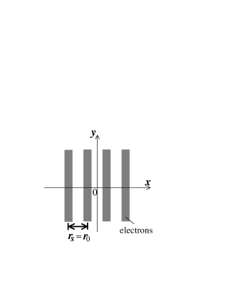
Figure 3.1: Schematic view of the density profile of the striped Hall state. The density of the striped Hall state is uniform in one direction and periodic with the period $r_{0}$ in the other direction. If we take the vNL asymmetry parameter $r_{s}=r_{0}$, the HF Hamiltonian is diagonalized on the vNL basis.

$$\langle\rho_{l}({\bf x})\rangle_{\rm stripe}=\sum_{N_{x}}\Delta_{l}(N_{x})F_{l}(\frac{2\pi N_{x}}{r_{0}},0)e^{i(2\pi N_{x}/r_{0})x},$$ (3.1)

where $r_{0}$ is the period of the density in the $x$-direction, $\Delta_{l}(N_{x})$ is an order parameter determined self-consistently, and $\Delta_{l}(0)=\nu^{\ast}$. Equation (3.1) gives the following form of the mean value of the projected density operator,

$$\langle\bar{\rho}_{l}({\bf k})\rangle_{\rm stripe}=\sum_{N_{x}}\Delta_{l}(N_{x})(2\pi)^{2}\delta(k_{x}+\frac{2\pi N_{x}}{r_{0}})\delta(k_{y}).$$ (3.2)

If we take the vNL asymmetry parameter $r_{s}=r_{0}$, Eq. (3.2) with $\tilde{\bf k}=(k_{x}/r_{s},r_{s}k_{y})$ takes the simple form,

$$\langle\bar{\rho}_{l}(\tilde{\bf k})\rangle_{\rm stripe}=\sum_{N_{x}}\Delta_{l}(N_{x})(2\pi)^{2}\delta(k_{x}+2\pi N_{x})\delta(k_{y}).$$ (3.3)

3.2.2 Diagonalization, eigenstates and eigenvalues

The HF Hamiltonian of the striped Hall state is already diagonalized on the vNL basis. Substitution of Eq. (3.3) into the HF Hamiltonian Eq. (2.41) gives the HF Hamiltonian for the striped Hall state by

$$\mathcal{H}_{\rm HF-stripe}^{(l)}=\int_{\rm BZ}\frac{d^{2}p}{(2\pi)^{2}}\epsilon_{l}({\bf p})b^{\dagger}_{l}({\bf p})b_{l}({\bf p}),$$ (3.4)

where $\epsilon_{l}({\bf p})$ is a one-particle energy given by

$$\epsilon_{l}({\bf p})=\epsilon^{(0)}_{l}+\sum_{N_{x}\neq 0}\Delta_{l}(N_{x})v_{l}^{\rm HF}(\frac{2\pi N_{x}}{r_{s}},0)(-1)^{N_{x}}e^{-iN_{x}p_{y}}.$$ (3.5)

In Eq. (3.5), $\epsilon^{(0)}_{l}$ is a uniform Fock energy given by $\nu^{\ast}v^{\rm HF}_{l}(0)$. The values of $v^{\rm HF}_{l}(0)$ are shown in Table 3.1.

$l$	$v^{\rm HF}_{l}(0)/(q^{2}/l_{\rm B})$
0	$-1.25331$
1	$-0.93999$
2	$-0.80290$
3	$-0.71968$

Table 3.1: Values of $v^{\rm HF}_{l}(0)$ for each LL.

For the ground state of the striped Hall state, the two-point function of the operator $b_{l}({\bf p})$ is given by [32, 33]

$$\langle b^{\dagger}_{l}({\bf p})b_{l^{\prime}}({\bf p}^{\prime})\rangle_{\rm stripe}= \sum_{\bf N}\delta_{l,l^{\prime}}\theta[\epsilon_{\rm F}-\epsilon_{l}({\bf p})](2\pi)^{2}\delta^{2}({\bf p}-{\bf p}^{\prime}-2\pi{\bf N})e^{-i\phi({\bf p},{\bf N})},$$ (3.6)

where $\epsilon_{\rm F}$ is a Fermi energy and $\theta$ is a step function.

3.2.3 Self-consistency condition and solution

The self-consistent equation for $\Delta_{l}(N_{x})$ is obtained by substitution of Eq. (3.6) into the left hand side of Eq. (3.3). $\Delta_{l}(N_{x})=(-1)^{N_{x}}\sin(\nu^{\ast}\pi N_{x})/\pi N_{x}$ is a solution of the self-consistent equation. This solution has the Fermi sea, $|p_{y}|<\pi\nu^{\ast}$ (shown in Fig. 3.2) and gives the one-particle energy as

$$\epsilon_{l}({\bf p})=\epsilon^{(0)}_{l}+\sum_{N_{x}\neq 0}v_{l}^{\rm HF}(\frac{2\pi N_{x}}{r_{s}},0)\frac{\sin(\nu^{\ast}\pi N_{x})}{\pi N_{x}}e^{-iN_{x}p_{y}}.$$ (3.7)

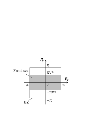
Figure 3.2: Fermi sea of the striped Hall state at $\nu^{\ast}$. The occupied state is represented by the dark region. When the stripe faces the $y$-direction, the $p_{x}$-direction of the Brillouin zone is fully occupied. In this case, the Fermi sea has the inter-LL energy gap in the $p_{x}$-direction and is gapless in the $p_{y}$-direction.

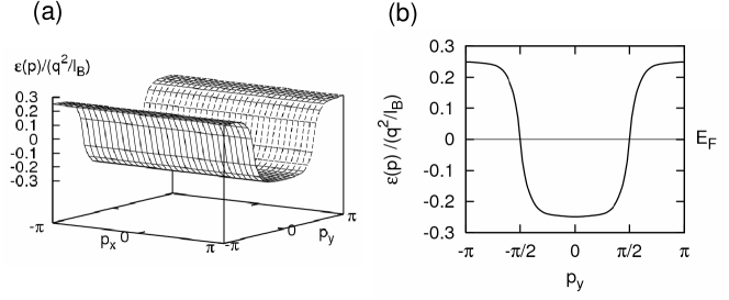
Figure 3.3: (a) 3D plot of the one-particle energy of the $l=2$ striped Hall state at half-filling. When the stripe faces the $y$-direction, the one-particle energy is uniform in the $p_{x}$-direction. (b) 2D plot of the one-particle energy as a function of $p_{y}$. The Fermi velocity is logarithmically divergent.

The HF energy per particle is given as a function of $r_{s}$ by

$$E_{\rm stripe}^{(l)}(r_{s})=\frac{\langle H_{\rm HF}^{(l)}\rangle_{\rm stripe}}{N_{e}^{(l)}}=\frac{\langle\mathcal{H}_{\rm HF-stripe}^{(l)}\rangle_{\rm stripe}}{2N_{e}^{(l)}}=\frac{1}{2}\epsilon^{(0)}_{l}+\frac{1}{2}\sum_{N_{x}\neq 0}\nu^{\ast}v_{l}^{\rm HF}(\frac{2\pi N_{x}}{r_{s}},0)\left(\frac{\sin(\nu^{\ast}\pi N_{x})}{\nu^{\ast}\pi N_{x}}\right)^{2}.$$ (3.8)

where $N_{e}^{(l)}$ is the total number of particles within the $l$th LL. We determine the optimal value of $r_{s}$ by minimizing $E_{\rm stripe}^{(l)}(r_{s})$ with respect to $r_{s}$. The optimal value of $r_{s}$ and the minimum energy at each LL are shown in Table 3.2 [33].

$l$	$r_{s}^{\rm stripe}$	$E_{\rm stripe}/(q^{2}/l_{\rm B})$
0	1.636	$-0.4331$
1	2.021	$-0.3490$
2	2.474	$-0.3074$
3	2.875	$-0.2800$

Table 3.2: Minimum energy and corresponding parameter $r_{s}$ of the striped Hall states at $\nu^{\ast}=1/2$.

For the optimal value of $r_{s}$, the one-particle energy and the density profile of the striped Hall state at $\nu^{\ast}=1/2$ in the $l=2$ LL are plotted in Fig. 3.3 and Fig. 3.4, respectively.

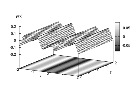
Figure 3.4: Density profile of the $l=2$ striped Hall state at half-filling. The uniform part $\rho_{0}=\nu^{\ast}$ is subtracted. The density of the striped Hall state is uniform in the $y$-direction and periodic with a period $r_{s}$ in the $x$-direction.

When the density is uniform in the $y$-direction, the one-particle energy is a function of only $p_{y}$ and uniform in the $p_{x}$-direction. The energy dispersion becomes gapless in the $p_{y}$-direction and has a inter-LL gap in the $p_{x}$-direction. The Fermi velocity $v_{F}=\partial\epsilon_{l}({\bf p})/\partial p_{y}|_{p_{y}=\pi\nu^{\ast}}$ is logarithmically divergent [32].

3.3 Charge density wave state

3.3.1 Assumption of the CDW density

Let us consider the case of $\nu^{\ast}$ in the $l$th LL. Here, we consider only the rectangular CDW state for simplicity. The CDW state has the following periodic density (Fig. 3.5),

Figure 3.5: Schematic view of the density of the rectangular CDW state. The density is periodic with the periodicity $r_{0x}$ and $r_{0y}$ in the $x$-direction and $y$-direction, respectively.

$$\langle\rho_{l}({\bf x})\rangle_{\rm CDW}=\sum_{\bf N}\Delta_{l}({\bf Q}_{\bf N})F_{l}({\bf Q}_{\bf N})e^{-i{\bf Q}_{\bf N}\cdot{\bf x}},$$ (3.9)

where ${\bf Q}_{\bf N}=(mQ_{0x},nQ_{0y})$ and ${\bf N}=(m,n)$ with integers $m$,$n$. Equation (3.9) gives the following form of the mean value of the projected density operator,

$$\langle\bar{\rho}_{l}({\bf k})\rangle_{\rm CDW}=\sum_{\bf N}\Delta_{l}({\bf Q}_{\bf N})(2\pi)^{2}\delta^{2}({\bf k}-{\bf Q}_{\bf N}).$$ (3.10)

The reciprocal vector ${\bf R}_{{\bf N}^{\prime}}$ is given by ${\bf R}_{{\bf N}^{\prime}}=2\pi(m^{\prime}/Q_{0x},n^{\prime}/Q_{0y})\equiv(m^{\prime}r_{0x},n^{\prime}r_{0y})$, which satisfies ${\bf Q}_{\bf N}\cdot{\bf R}_{{\bf N}^{\prime}}=2\pi M$ with an integer $M$. Since one electron in the CDW state with the density Eq. (3.9) occupies the area $S_{0}=r_{0x}r_{0y}$ and one state in each LL occupies the area $S_{\phi}=a^{2}$ with the vNL constant $a=\sqrt{h/eB}$, the partial filling factor $\nu^{\ast}$ is given by

$$\nu^{\ast}=\frac{\hbox{Number of electrons in the $l$th LL}}{\hbox{\rm Number of states in one LL}}=\frac{a^{2}}{r_{0x}r_{0y}}.$$ (3.11)

Thus, the relation $r_{0x}=a^{2}/\nu^{\ast}r_{0y}$ holds. In particular, in the case of $\nu^{\ast}=N/M$, this relation is given by $r_{0x}=M/Nr_{0y}$, where we set $a=1$ and the integers $M$,$N$ have no factors in common. By using this relation, ${\bf Q}_{\bf N}$ is rewritten as

$${\bf Q}_{\bf N}=(\frac{2\pi m}{r_{0x}},2\pi nr_{0x}\frac{N}{M}).$$ (3.12)

Hence, $\langle\bar{\rho}_{l}({\bf k})\rangle_{\rm CDW}$ is given by

$$\langle\bar{\rho}_{l}({\bf k})\rangle_{\rm CDW}=\sum_{m,n}\Delta_{l}({\frac{2\pi m}{r_{0x}},2\pi nr_{0x}\nu^{\ast}})(2\pi)^{2}\delta(k_{x}-\frac{2\pi m}{r_{0x}})\delta(k_{y}-2\pi nr_{0x}\nu^{\ast}),$$ (3.13)

with $\nu^{\ast}=M/N$. If we take $r_{s}=r_{0x}$ (Fig. 3.6), $\langle\bar{\rho}_{l}(\tilde{\bf k})\rangle_{\rm CDW}$ is given by

$$\langle\bar{\rho}_{l}(\tilde{\bf k})\rangle_{\rm CDW}= \sum_{m,n}\Delta_{l}({\frac{2\pi m}{r_{s}},2\pi nr_{s}\nu^{\ast}})(2\pi)^{2}\delta(k_{x}-2\pi m)\delta(k_{y}-2\pi n\nu^{\ast})$$

$$= \sum_{m,j=-\infty}^{\infty}\sum_{k=0}^{M-1}\Delta_{l}(\frac{2\pi m}{r_{s}},2\pi r_{s}(jM+k)\frac{N}{M})(2\pi)^{2}\delta(k_{x}-2\pi m)\delta(k_{y}-2\pi(jM+k)\frac{N}{M}),$$ (3.14)

where $n=jM+k$ with integers $j,k$ ($k=0,1,2,\dots,M-1$).

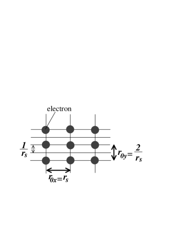
Figure 3.6: The vNL unit cell and the CDW unit cell in the case of $\nu^{\ast}=1/2$. The thin lines represent the vNL. For $\nu^{\ast}=1/2$, the CDW unit cell is just twice as large as the vNL unit cell. If we take $r_{s}=r_{0x}$, the HF Hamiltonian can be block-diagonalized.

3.3.2 Diagonalization, eigenstates and eigenvalues

Substituting Eq. (3.14) into the HF Hamiltonian Eq. (2.41), we can block-diagonalized the HF Hamiltonian as follows. Under the assumption Eq. (3.9) at $\nu^{\ast}=N/M$, the HF Hamiltonian is written as

$$\mathcal{H}_{\rm HF-CDW}^{(l)}= \int\frac{d^{2}k}{(2\pi)^{2}}v_{l}^{\rm HF}(\tilde{\bf k})$$

$$\times\sum^{\infty}_{m,j=-\infty}\sum^{M-1}_{k=0}\Delta_{l}(\frac{2\pi m}{r_{s}},2\pi r_{s}(jM+k)\frac{N}{M})(2\pi)^{2}\delta(k_{x}+2\pi m)\delta(k_{y}+2\pi(jM+k)\frac{N}{M})\bar{\rho}_{l}(\tilde{\bf k}),$$

$$= \epsilon_{l}^{(0)}N_{e}^{(l)}+\sum^{\infty}_{m,j=-\infty}\sum^{M-1}_{k=0}\Delta_{l}^{\rm HF}(m;j,k)\bar{\rho}_{l}(-\frac{2\pi m}{r_{s}},-2\pi r_{s}(jM+k)\frac{N}{M}),$$ (3.15)

where

$$\Delta_{l}^{\rm HF}(m;j,k)\equiv\Delta_{l}(\frac{2\pi m}{r_{s}},2\pi r_{s}(jM+k)\frac{N}{M})v_{l}^{\rm HF}(-\frac{2\pi m}{r_{s}},-2\pi r_{s}(jM+k)\frac{N}{M}),$$ (3.16)

except for $m=j=k=0$ and $\Delta_{l}^{{\rm HF}}(0;0,0)=0$. Substituting Eq. (2.40) into Eq. (3.15) and using the boundary condition of $b_{l}({\bf p})$ given in Eq. (2.29), we rewrite the HF Hamiltonian as

$$\mathcal{H}_{\rm HF-CDW}^{(l)}-\epsilon_{l}^{(0)}N_{e}^{(l)}= \int_{\rm BZ}\frac{d^{2}p}{(2\pi)^{2}}\sum^{\infty}_{m,j=-\infty}\sum^{M-1}_{k=0}\Delta_{l}^{\rm HF}(m;j,k)e^{i\pi(m+jN+m(j+k/M)N)}$$

$$\times b_{l}^{\dagger}({\bf p})b_{l}(p_{x},p_{y}+2\pi k\frac{N}{M})e^{imp_{y}-i(jN)p_{x}}.$$ (3.17)

Here, if we divide the interval of the $p_{y}$-integral into $M$ same intervals and reduce each interval to the range $[0,2\pi/M]$ using the boundary condition Eq.(2.29), $\mathcal{H}_{\rm HF-CDW}^{(l)}$ is given by

$$\mathcal{H}_{\rm HF-CDW}^{(l)}-\epsilon_{l}^{(0)}N_{e}^{(l)}= \int^{2\pi}_{0}\frac{dp_{x}}{2\pi}\int^{2\pi/M}_{0}\frac{dp_{y}}{2\pi}\sum^{\infty}_{m,j=-\infty}\sum^{M-1}_{k,k^{\prime}=0}\Delta_{l}^{\rm HF}(m;j,k-k^{\prime})e^{i\pi(m+jN+m(j+(k-k^{\prime})/M)N)}$$

$$\times b_{l}^{\dagger}(p_{x},p_{y}+2\pi k^{\prime}\frac{N}{M})b_{l}(p_{x},p_{y}+2\pi k\frac{N}{M})e^{imp_{y}-i(jN)p_{x}+i2\pi mk^{\prime}N/M}$$

$$= \int^{2\pi}_{0}\frac{dp_{x}}{2\pi}\int^{2\pi/M}_{0}\frac{dp_{y}}{2\pi}\sum^{M-1}_{k,k^{\prime}=0}b_{l}^{\dagger}({\bf p},k^{\prime})\Delta_{l}^{\rm HF}({\bf p},k^{\prime},k)b_{l}({\bf p},k),$$ (3.18)

where

$$b({\bf p},k)\equiv b(p_{x},p_{y}+2\pi k\frac{N}{M}),$$ (3.19)

$$\Delta_{\rm HF}({\bf p},k^{\prime},k)\equiv\sum^{\infty}_{m=-\infty}\sum^{\infty}_{j=-\infty}\Delta_{\rm HF}(m;j,k-k^{\prime})e^{i\pi(m+jN+m(j+(k+k^{\prime})/M)N)}e^{imp_{y}-i(jN)p_{x}}.$$ (3.20)

Hence, the HF Hamiltonian $\mathcal{H}_{\rm HF-CDW}^{(l)}$ is block-diagonalized and the problem is reduced to the diagonalization problem of the $M\times M$ Hermite matrix $\Delta_{l}^{\rm HF}({\bf p},k^{\prime},k)$. Note that the fact that $\langle\rho_{l}({\bf r})\rangle$ is real gives the relation $\Delta_{l}^{\ast}(-{\bf Q}_{N})=\Delta_{l}({\bf Q}_{N})$, and by using this relation, it is proved that the $M\times M$ matrix ${\bf\Delta}_{l}^{\rm HF}({\bf p})$ with $\{{\bf\Delta}^{\rm HF}_{l}({\bf p})\}_{k^{\prime},k}\equiv\Delta_{\rm HF}({\bf p},k^{\prime},k)$ is Hermite.

The Hermite matrix ${\bf\Delta}_{l}^{\rm HF}({\bf p})$ is diagonalized using the unitary matrix $U({\bf p})$ as

$$\Lambda({\bf p})=U^{\dagger}({\bf p}){\bf\Delta}_{l}^{\rm HF}({\bf p})U({\bf p})=\left(\begin{array}[]{cccc}\epsilon_{0}({\bf p})&&&\\ &\epsilon_{1}({\bf p})&&\\ &&\ \ddots&\\ &&&\epsilon_{M-1}({\bf p})\\ \end{array}\right),$$ (3.21)

here, $\epsilon_{s}({\bf p})$ represents the eigenvalue of the $(s+1)$th energy band, and the eigenvector for $\epsilon_{s}$ is given by $\{{\bf v}_{s}({\bf p})\}_{s^{\prime}}=U_{s,s^{\prime}}({\bf p})$. ${\rm RBZ}$ represents the reduced Brillouin zone, $0<p_{x}<2\pi$, $0<p_{y}<2\pi/M$. Hence, the HF Hamiltonian $\mathcal{H}_{\rm HF-CDW}^{(l)}$ is diagonalized as

$$\mathcal{H}_{\rm HF-CDW}^{(l)}-\epsilon_{l}^{(0)}N_{e}^{(l)}=\int_{\rm RBZ}\frac{d^{2}p}{(2\pi)^{2}}{\bf c}_{l}^{\dagger}({\bf p})\Lambda({\bf p}){\bf c}_{l}({\bf p})=\int_{\rm RBZ}\frac{d^{2}p}{(2\pi)^{2}}\sum_{s=0}^{M-1}\epsilon_{s}({\bf p})c^{\dagger}_{s}({\bf p})c_{s}({\bf p}),$$ (3.22)

where

$${\bf c}_{l}({\bf p})=(c_{0}({\bf p}),c_{1}({\bf p}),\cdots,c_{M-1}({\bf p}))^{t}=U^{\dagger}({\bf p}){\bf b}_{l}({\bf p})\quad{\rm with}$$

$$\{{\bf b}_{l}({\bf p})\}_{k}=b_{l}({\bf p},k),\quad c_{s}({\bf p})=\sum_{k=0}^{M-1}U^{\dagger}_{s,k}({\bf p})b_{l}({\bf p},k).$$ (3.23)

In the present case of $\nu^{\ast}=N/M$, the lower N bands (from $s=0$ to $s=N-1$) are fully occupied for the ground state.

3.3.3 Self-consistency condition

The HF Hamiltonian should be diagonalized self-consistently. The ground state is given by

$$|\Omega\rangle=N_{c}\prod_{s=0}^{N-1}\prod_{{\bf p}\in{\rm RBZ}}c_{s}^{\dagger}({\bf p})|0\rangle,$$ (3.24)

where $N_{c}$ is a normalization constant and $|0\rangle$ is a vacuum state in which the $(l-1)$th and lower Landau levels are fully occupied. Using this ground state, we obtain the self-consistency condition

$$\langle\Omega|\bar{\rho}_{l}({\bf q})|\Omega\rangle=\sum_{\bf N}\Delta_{l}({\bf Q}_{\bf N})(2\pi)^{2}\delta^{2}({\bf q}-{\bf Q}_{\bf N}).$$ (3.25)

In what follows, we derive the self-consistent equation for $\Delta({\bf Q}_{\bf N})$ from Eq.(3.25).

The field operators $b_{l}^{\dagger}({\bf p})$ and $b_{l}({\bf p})$ satisfy the anti-commutation relation Eq. (2.30). For ${\bf p}$ and ${\bf p}^{\prime}$ within the RBZ, Eq. (2.30) becomes

$$\{b_{l}^{\dagger}({\bf p},k),b_{l^{\prime}}({\bf p}^{\prime},k^{\prime})\}=(2\pi)^{2}\delta_{l,l^{\prime}}\delta_{k,k^{\prime}}\delta^{2}({\bf p}-{\bf p}^{\prime}).$$ (3.26)

For $c_{s}^{\dagger}({\bf p})$ and $c_{s}({\bf p})$, the corresponding relation is given by

$$\{c^{\dagger}_{s}({\bf p}),c_{s^{\prime}}({\bf p}^{\prime})\}=\delta_{s,s^{\prime}}(2\pi)^{2}\delta^{2}({\bf p}-{\bf p}^{\prime}).$$ (3.27)

Using Eq. (2.40), we rewrite the self-consistency condition Eq. (3.25) as

$$\langle\Omega|b_{l}^{\dagger}({\bf p})b_{l}({\bf p}^{\prime})|\Omega\rangle=\sum^{M-1}_{k=0}F({\bf p},k)\sum_{\bf N}(2\pi)^{2}\delta(p_{x}-p_{x}^{\prime}-2\pi N_{x})\delta(p_{y}-p_{y}^{\prime}-2\pi N_{y}-2\pi k\frac{N}{M})e^{-i\phi({\bf p},{\bf N})},$$ (3.28)

where

$$F({\bf p},k)=\sum_{m,j=-\infty}^{\infty}\Delta_{l}(\frac{2\pi m}{r_{s}},2\pi r_{s}(jM+k)\frac{N}{M})e^{-i\pi(m+jN)-i\pi m(j+k/M)N}.$$ (3.29)

The left hand side of Eq. (3.28) is calculated using Eqs. (3.23) and (3.27), and the result is

$$\langle\Omega|b_{l}^{\dagger}({\bf p},k)b_{l}({\bf p}^{\prime},0)|\Omega\rangle=\left(\sum_{s=0}^{N-1}U^{\dagger}_{s,k}({\bf p})U_{0,s}({\bf p})\right)(2\pi)^{2}\delta^{2}({\bf p}-{\bf p}^{\prime}),$$ (3.30)

for ${\bf p}$ and ${\bf p}^{\prime}$ within the RBZ. From Eqs. (3.25) and (3.30), the self-consistent equation for $\Delta_{l}({\bf Q}_{N})$ is given by

$$\Delta_{l}(\frac{2\pi m}{r_{s}},2\pi r_{s}(jM+k)\frac{N}{M})=\int_{BZ}\frac{d^{2}p}{(2\pi)^{2}}\left(\sum_{s=0}^{N-1}U^{\dagger}_{s,k}({\bf p})U_{0,s}({\bf p})\right)e^{ip_{x}(jN)-imp_{y}}e^{i\pi(m+jN)+i\pi m(j+k/M)N}.$$ (3.31)

If the right hand side of Eq. (3.31) coincides with the left hand side, the problem is self-consistently solved.

3.3.4 Density profile and Energy dispersion of CDW states

As in the case of the striped Hall state, the HF energy per particle is given as a function of $r_{s}$ by

$$E_{\rm CDW}^{(l)}(r_{s})=\frac{\langle H_{\rm HF}^{(l)}\rangle_{\rm CDW}}{N_{e}^{(l)}}=\frac{1}{2}\epsilon_{l}^{(0)}+\frac{1}{2}\int^{2\pi}_{0}\frac{dp_{x}}{2\pi}\int^{2\pi/M}_{0}\frac{dp_{y}}{\left(\frac{2\pi}{M}\right)}\sum^{N-1}_{s=0}\epsilon_{s}({\bf p}).$$ (3.32)

The optimal value of $r_{s}$ is determined by minimization of $E_{\rm CDW}^{(l)}(r_{s})$ to $r_{s}$. The optimal value of $r_{s}$ and the minimum energy per particle at several fillings in $l=0,2$ are shown in Table 3.3 and Fig. 3.8, where cohesive energy, which is defined as $\hbox{(Total energy)}-\hbox{(Uniform Fock energy)}$, is shown for the minimum energy. As for $l=0$ LL, the optimal value of $r_{s}$ is approximately given by $\sqrt{1/\nu^{\ast}}$, which gives $r_{0x}=r_{0y}$. Hence, the CDW states in the $l=0$ LL become isotropic for the $x$ and $y$-directions. On the other hand, as for the $l=2$ LL, the optimal value of $r_{s}$ takes a different value from $1/\nu^{\ast}$ especially near $\nu^{\ast}=1/2$, which means that anisotropic states are energetically favorable at these fillings. Hence, the CDW states in the $l=2$ LL become anisotropic near $\nu^{\ast}=1/2$. Since the original Hamiltonian has a rotational symmetry, the direction of the anisotropy can take any direction. In the present case of the rectangular vNL, two solutions whose anisotropy direction in density face the $x$ or $y$-direction are degenerate. This degeneracy yields two optimal values of $r_{s}$ for anisotropic states. When we set the smaller one to $r_{s}^{(1)}$ and the larger one to $r_{s}^{(2)}$, they are related by

$$r_{s}^{(1)}=\frac{1}{\nu^{\ast}r_{s}^{(2)}}.$$ (3.33)

Only the smaller value $r_{s}^{(1)}$ is shown in Table 3.3 as the optimal value of $r_{s}$ for the CDW states in the $l=2$ LL.

The density profile of the CDW state is given by

$$\langle\rho_{l}({\bf x})\rangle_{\rm CDW}=\sum^{\infty}_{m,n=-\infty}\Delta_{l}(\frac{2\pi m}{r_{s}},2\pi r_{s}n\frac{N}{M})F_{l}(\frac{2\pi m}{r_{s}},2\pi r_{s}n\frac{N}{M})\cos(\frac{2\pi m}{r_{s}}x+2\pi r_{s}n\frac{N}{M}y),$$ (3.34)

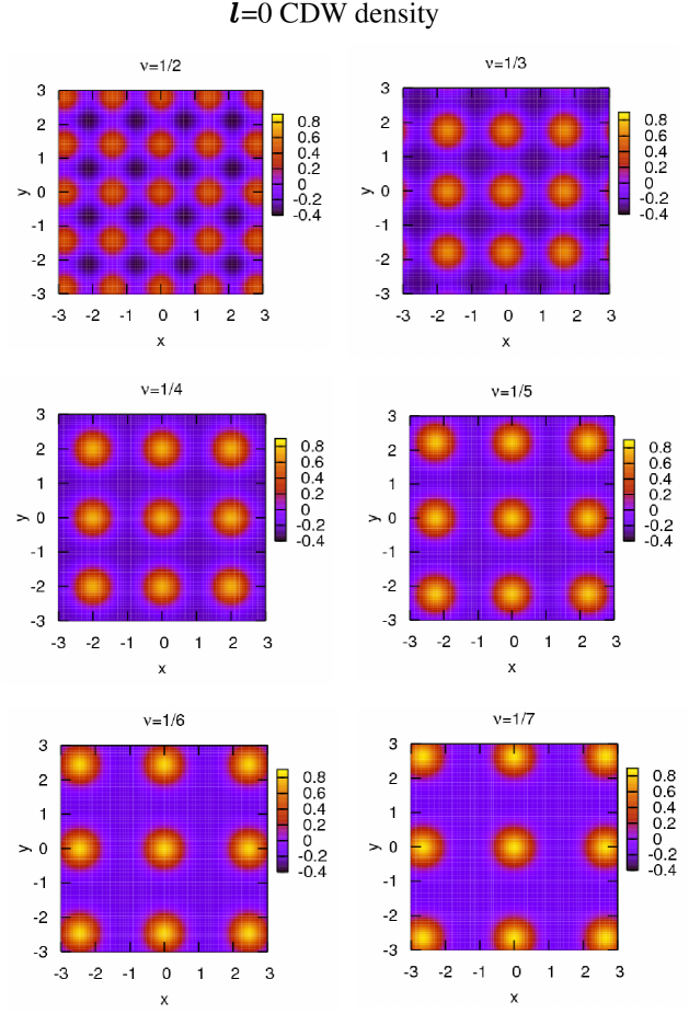
Figure 3.9: 2D plot of the density of the $l=0$ CDW state. As the filling decreases, the distance between localized electrons increases isotropically.

where the $x$ and $y$-inversion symmetry is assumed. In Figs. 3.9 and 3.10, the density profile is plotted at several fillings in $l=0,2$ LLs for the optimal value of $r_{s}$. As for the $l=0$ CDW density, the density becomes isotropic for all partial fillings. On the other hand, as for the $l=2$ CDW density, the density becomes highly anisotropic near $\nu^{\ast}=1/2$, and as the partial filling decreases, the density approaches the isotropic one gradually. This difference between the lowest LL and the higher LLs is mainly due to the difference of the form of the HF potential $v_{l}^{\rm HF}({\bf k})$. We refer to the direction with a narrower periodicity in density as “stripe direction” in this thesis.

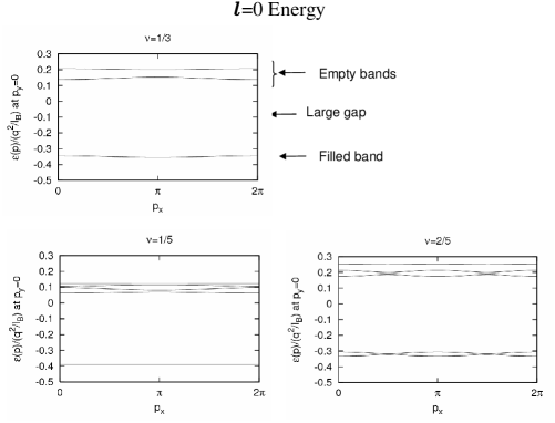
Figure 3.11: 2D plot of the one-particle energy dispersion of the $l=0$ CDW state. The energy dispersion at $p_{y}=0$ is plotted as a function of $p_{x}$. There is a large gap between the filled bands and the empty bands.

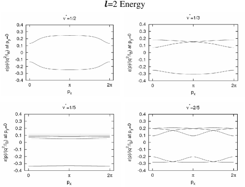
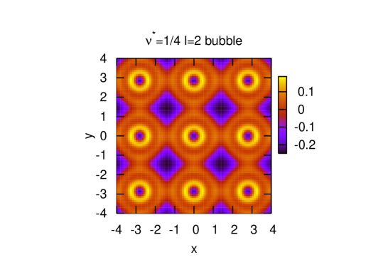
Figure 3.12: 2D plot of the one-particle energy dispersion of the $l=2$ CDW state. The energy dispersion at $p_{y}=0$ is plotted as a function of $p_{x}$. There is a large gap between the filled bands and the empty bands.

In the present vNL formalism, the energy dispersion of the CDW state is obtained as a function of momenta $p_{x}$ and $p_{y}$ which are conjugate to the vNL. As for the $l=0$ LL, the energy dispersion is isotropic in the $p_{x}$ and $p_{y}$-directions and the band width becomes narrower as the density becomes lower. In Fig. 3.11, the energy dispersion at $p_{y}=0$ is plotted as a function of $p_{x}$. As for the $l=2$ LL, the energy dispersion becomes almost flat in the direction perpendicular to the stripe direction. In Fig. 3.12, the energy dispersion at $p_{y}=0$ is plotted as a function of $p_{x}$. In both cases, there is a large energy gap between the filled bands and the empty bands. This large gap coincides with the previously obtained results by Yosioka and Lee [26].

3.4 Bubble state

3.4.1 Assumption of the bubble density

The bubble state is a CDW state with two or more electrons per unit cell. We call the bubble state with $N$ electrons per unit cell the “$N$-electron bubble state”. Let us consider the $N$-electron rectangular bubble state at $\nu^{\ast}=1/M$ in the $l$th LL, with a period $r_{0x}$ and $r_{0y}$ in the $x$ and $y$ direction, respectively. In this case, since $N$ electrons are in the area of the unit cell $S_{0}=r_{0x}r_{0y}$ and the density of states is given by $1/a^{2}$, the partial filling factor is given by

$$\nu^{\ast}=\frac{\hbox{Number of electrons in the $l$th LL}}{\hbox{Number of states in one LL}}=\frac{\frac{L_{x}L_{y}}{r_{0x}r_{0y}}N}{\frac{L_{x}L_{y}}{a^{2}}}=\frac{a^{2}}{r_{0x}r_{0y}}N,$$ (3.35)

where $L_{x}$ and $L_{y}$ are the size of the system in the $x$ and $y$ directions, respectively. In particular, in the case of $\nu^{\ast}=1/M$, this relation becomes $r_{0x}=NM/r_{0y}$, where we set $a=1$. By using this relation, the mean value of the projected density operator of the $N$-electron bubble state is given by

$$\langle\bar{\rho}_{l}(\tilde{\bf k})\rangle_{\rm bubble}=\sum_{m,n=-\infty}^{\infty}\Delta_{l}(\frac{2\pi m}{r_{s}},2\pi nr_{s}\frac{1}{NM})(2\pi)^{2}\delta(k_{x}-2\pi m)\delta(k_{y}-2\pi n\frac{1}{NM}),$$ (3.36)

where we set $r_{s}=r_{0}$. Hence, the diagonalization procedure of the HF Hamiltonian is the same as in the case of the CDW state at $\nu^{\ast}=1/K$ with $K=NM$.

3.4.2 Self-consistency condition and solution

The important difference from the CDW state is a self-consistency condition. The one-particle energy of the $N$-electron bubble state at $\nu^{\ast}=1/M$ has $K=NM$ energy bands. Since the filling factor is $1/M$, the lowest $N$ bands are fully occupied for the ground state. As a result, the self-consistency condition is given by

$$\Delta_{l}(\frac{2\pi m}{r_{s}},2\pi(n+\frac{j}{K})r_{s})=\int_{\rm BZ}\frac{d^{2}p}{(2\pi)^{2}}\left(\sum^{N-1}_{s=0}U^{\ast}_{j,s}({\bf p})U_{0,s}({\bf p})\right)(-1)^{m+n+mn}e^{ip_{x}n-ip_{y}m-i\pi m(j/K)}.$$ (3.37)

For the $l=0$ LL, no self-consistent bubble solution has been obtained. For the $l=2$ LL, a self-consistent bubble solution is obtained for $\nu^{\ast}=1/4$. The obtained solution is a 2-electron bubble state. The optimal value of $r_{s}$ is $r_{s}=2.8$ and the corresponding cohesive energy is $-0.1576$ $(q^{2}/l_{\rm B})$ which is slightly lower than that of the CDW state at the same filling. Hence, for the $\nu^{\ast}=1/4$ in the $l=2$ LL, the 2-electron bubble state is more stable. The density profile of this state is shown in Fig. 3.13, which is almost isotropic. The energy dispersion consists of eight bands and the lower two bands are fully occupied. As in the case of the CDW state, there is a large gap between the filled bands and the empty bands.

Since electrons of this 2-electron bubble state are well-localized in density, it is expected that the state is easily pinned by impurities, which results in a quantization of the Hall conductivity owing to its collective insulating property. Indeed, this quantization has been observed around $\nu^{\ast}=1/4,3/4$ in the $l=2$ LL [10, 11], and it is believed that this observed quantization is an evidence of the bubble state.

3.4.3 Relation between the $N$-electron bubble state and the CDW state at $\nu^{\ast}=1/M$

The diagonalization formalism for the $N$-electron bubble state at $\nu^{\ast}=1/M$ includes the CDW solution at $\nu^{\ast}=1/M$. To make this point clear, let us compare the mean value of the density of the CDW state and the bubble state. For the CDW state at $\nu^{\ast}=1/M$, the mean values of the density operators are given by

$$\langle\rho_{l}({\bf x})\rangle_{\rm CDW}=\sum^{\infty}_{m,n=-\infty}\Delta_{l}^{\rm CDW}(\frac{2\pi m}{r_{\rm C}},2\pi r_{\rm C}n\frac{1}{M})F_{l}(\frac{2\pi m}{r_{\rm C}},2\pi r_{\rm C}n\frac{1}{M})e^{-i(2\pi m/r_{\rm C})x-i(2\pi r_{\rm C}/M)y},$$ (3.38)

$$\langle\bar{\rho}_{l}(\tilde{\bf k})\rangle_{\rm CDW}=\sum^{\infty}_{m,n=-\infty}\Delta_{l}^{\rm CDW}(\frac{2\pi m}{r_{\rm C}},\frac{2\pi r_{\rm C}n}{M})(2\pi)^{2}\delta(k_{x}-2\pi m)\delta(k_{y}-2\pi n\frac{1}{M}),$$ (3.39)

and for the $N$-electron bubble state at $\nu^{\ast}=1/M$, they are given by

$$\langle\rho_{l}({\bf x})\rangle_{\rm bubble}=\sum^{\infty}_{m,n=-\infty}\Delta_{l}^{\rm bubble}(\frac{2\pi m}{r_{\rm B}},2\pi r_{\rm B}n\frac{1}{K})F_{l}(\frac{2\pi m}{r_{\rm B}},2\pi r_{\rm B}n\frac{1}{K})e^{-i(2\pi m/r_{\rm B})x-i(2\pi r_{\rm B}n/K)y},$$ (3.40)

$$\langle\bar{\rho}_{l}(\tilde{\bf k})\rangle_{\rm bubble}=\sum^{\infty}_{m,n=-\infty}\Delta_{l}^{\rm bubble}(\frac{2\pi m}{r_{\rm B}},\frac{2\pi r_{\rm B}n}{K})(2\pi)^{2}\delta(k_{x}-2\pi m)\delta(k_{y}-2\pi n\frac{1}{K}),$$ (3.41)

with $K=MN$, where $r_{s}=r_{\rm C}$ for the CDW state and $r_{s}=r_{\rm B}$ for the bubble state.

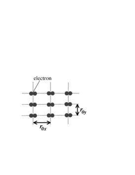
Figure 3.7: Schematic view of the density of the 2-electron bubble state.

If we set $r_{\rm B}=Nr_{\rm C}$, $\Delta_{l}^{\rm bubble}(2\pi Nm/r_{\rm B},2\pi r_{\rm B}n/K)=\Delta_{l}^{\rm CDW}(2\pi m/r_{\rm C},2\pi r_{\rm C}n/M)$ and other $\Delta_{l}^{\rm bubble}$s is equal to zero, $\langle\rho_{l}({\bf x})\rangle_{\rm bubble}$ becomes the same as $\langle\rho_{l}({\bf x})\rangle_{\rm CDW}$. Hence, the HF Hamiltonian with the assumption (3.36) becomes the same as the HF Hamiltonian with the assumption (3.14).

$\nu^{\ast}(l=0)$	$r_{s}^{\rm CDW}$	$E_{\rm CDW}/(q^{2}/l_{\rm B})$
1/2	1.41	$-0.1303$
3/7	1.52	$-0.1516$
2/5	1.58	$-0.1597$
1/3	1.73	$-0.1768$
2/7	1.87	$-0.1866$
1/4	2.00	$-0.1918$
1/5	2.24	$-0.1943$
1/6	2.45	$-0.1920$
1/7	2.65	$-0.1880$
1/10	3.16	$-0.1739$
$\nu^{\ast}(l=2)$	$r_{s}^{\rm CDW}$	$E_{\rm CDW}/(q^{2}/l_{\rm B})$
1/2	0.82	$-0.1090$
3/7	0.96	$-0.1245$
2/5	1.03	$-0.1304$
1/3	1.22	$-0.1426$
2/7	1.44	$-0.1498$
1/4	1.67	$-0.1550$
1/5	2.24	$-0.1672$
1/6	2.45	$-0.1757$
1/7	2.65	$-0.1791$
1/10	3.16	$-0.1748$

Table 3.3: Minimum energy and corresponding parameter $r_{s}$ of the CDW states at several fillings in the $l=0,2$ LL. As for the minimum energy, the uniform Fock energy is subtracted. The optimal value of $r_{s}$ for the $l=2$ LL takes two different values which give the same energy. Only the smaller one is shown in this table. These values are plotted in Fig. 3.8

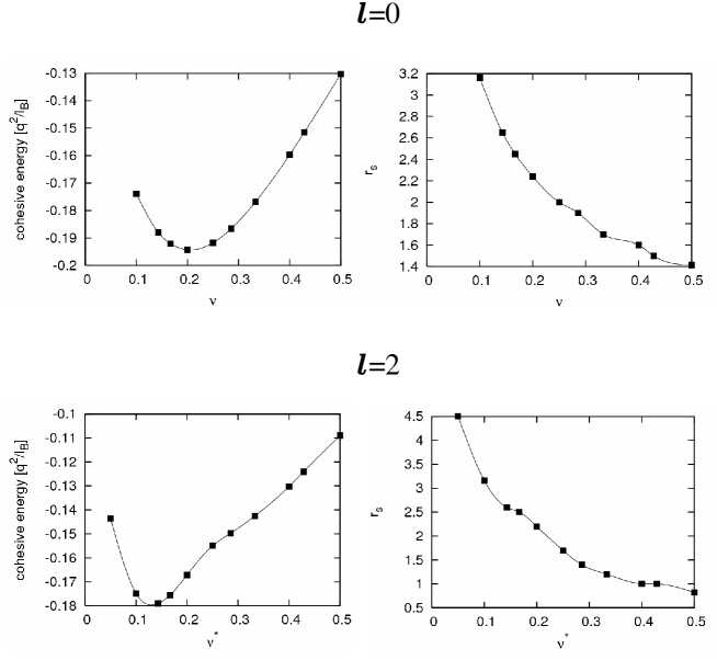
Figure 3.8: The optimal value of $r_{s}$ is plotted for $l=2$ CDW states. Cohesive energy is plotted for $l=0$ CDW states with the optimal value of $r_{s}$.

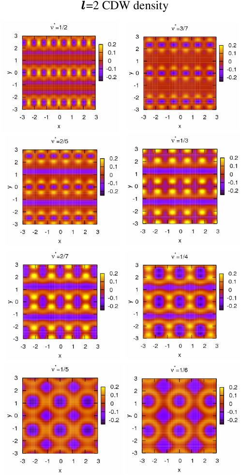
Figure 3.10: 2D plot of the density of the $l=2$ CDW state. Near $\nu^{\ast}=1/2$, the density is highly anisotropic. As $\nu^{\ast}$ decreases, the density becomes isotropic gradually.

Figure 3.13: 2D plot of the density of the $l=2$ 2-electron bubble state at $\nu^{\ast}=1/4$. The density is almost isotropic in the $x$ and $y$ directions.

Figure 3.14: 2D plot of the one-particle energy dispersion of the $l=2$ 2-electron bubble state at $\nu^{\ast}=1/4$. The energy dispersion at $p_{y}=0$ is plotted as a function of $p_{x}$. There is a large gap between the filled bands and the empty bands.

Chapter 4 Effects of an injected current on highly anisotropic states

In this chapter, we study effects of an injected current on highly anisotropic states which have been discovered around half-filled third and higher Landau levels (LLs) in experiments with ultra-high mobility samples at low temperatures. While several states have been proposed to theoretically explain the experimental results so far, it is still an open problem which state is realized in the experiments. Most previous studies have been done within the Hartree-Fock (HF) approximation with no injected current. In experiments of anisotropic states, however, a current is injected to investigate properties of the system. This effect has not been taken into account in the previous studies. In this chapter, we focus on two different anisotropic HF states, i.e., a striped Hall state and an anisotropic charge density wave (ACDW) state, and investigate the effect of the injected current on these two HF states using response functions against the injected current. The calculations are done by means of a von Neumann lattice (vNL) formalism developed in Chapter 2. With no injected current, the ACDW state has a lower energy. We find that the striped Hall state becomes lower energy state when the injected current exceeds a critical value. The critical value is estimated at about $0.04$-$0.05$ nA, which is much smaller than the current used in experiments of anisotropic states.

4.1 Introduction

In the quantum Hall system, half-filled states at each Landau level (LL) exhibit much attractive features. Around the half-filled lowest LL, isotropic compressible states have been observed [36, 37], which are widely believed to be the Fermi liquid of composite fermions. Around the half-filled second LL, the $5/2$ fractionally quantized Hall conductance has been observed [38]. The p-wave Cooper pairing state of composite fermions, which is called the Pfaffian state, has been proposed to explain this state [39, 40]. Around half-filled third and higher LLs, highly anisotropic states, which have extremely anisotropic longitudinal resistivities and un-quantized Hall resistivities, have been found in ultra-high mobility samples at low temperatures [9, 10]. Much theoretical work has been done to study the anisotropic states [8, 41, 42, 43, 44, 45, 46, 47, 48, 49, 34, 28] and several states have been proposed so far. In this chapter, we focus on two different HF states among them, i.e., a striped Hall state [8, 41] and an anisotropic charge density wave (ACDW) state [28].

The striped Hall state is a unidirectional charge density wave state which is a gapless state with an anisotropic Fermi surface [32, 33]. The Fermi surface has an energy gap in one direction and is gapless in the other direction (Figs. 3.2 and 4.1). The ACDW state is a CDW state which has a similar periodic density in a direction perpendicular to stripes, and in addition, has a density modulation along stripes (Fig. 4.2). The density modulation along stripes results in energy gaps in both directions. These features suggest that the anisotropic state found in experiments is the striped Hall state since the anisotropic longitudinal resistivity and the un-quantized Hall resistivity are naturally explained by the anisotropic Fermi surface [32, 33], while it is difficult to explain these experimental features with the ACDW state because of the energy gap. However, it has been pointed out that the striped Hall state is unstable within the HF approximation to formation of modulations along stripes so that the ACDW state is the lower energy state [28]. This has been an enigma as to the anisotropic states.

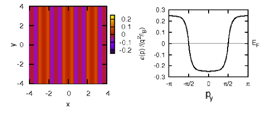
Figure 4.1: Left: Density modulation of the striped Hall state at the half-filled third LL. The uniform part is subtracted. The density is periodic in the $x$-direction and uniform in the $y$-direction (stripe direction). The injected current flows easily in the stripe direction. Right: Energy spectrum of the striped Hall state at the same filling. It is uniform in the $p_{x}$-direction. The BZ is $|p_{i}|<\pi$ and $E_{F}$ is a Fermi energy.

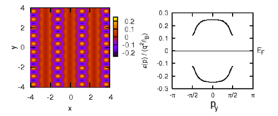
Figure 4.2: Left: Density modulation of the ACDW state at the half-filled third LL. The uniform part is subtracted. The density is modulated along stripes. Right: Energy spectrum of the ACDW state at the same filling. It depends on $p_{x}$ weakly and the spectrum at $p_{x}=0$ is plotted. The BZ is reduced to $|p_{y}|<\pi/2$ owing to the modulations along stripes and the two bands are formed.

In the experiments of the anisotropic states, current is injected. This effect has not been taken into account in the previous calculations of the total energy. About two decades ago, MacDonald et al. have studied the effect of the injected current on the integer quantum Hall system [50]. They calculated the current and charge distributions and found that charges accumulate around both edges of the sample with the opposite sign, as expected from the classical Hall effect [50, 51, 52, 53]. The charge accumulation causes the energy enhancement via the Coulomb interaction between charged particles. The same type of energy corrections may exist even in the present highly correlated quantum Hall states. However, the effect of the injected current on the anisotropic state has not been studied.

In this chapter, we calculate the correlation energies of the striped Hall state and the ACDW state in the system with the injected current flowing in the direction along stripes, and with no impurities and no metallic contacts. It is important to know if the ACDW state has a lower energy even in the system with the injected current. The density modulation along stripes shown in Fig. 4.2 suggest that the effect of the injected current becomes larger in the ACDW state. To verify whether this naive expectation is true or not, the dependence of the correlation energies on the injected current is studied in detail. Effects of impurities and metallic contacts are ignored in our calculations of correlation energies since these effects are expected to be small in experiments of anisotropic states in ultra-high mobility samples and are outside the scope of this work. Effects of the injected current are investigated using response functions for electromagnetic fields. The current and charge distributions are determined and energies of the two states are calculated from these distributions. It is found that the energy of the ACDW state increases faster than that of the striped Hall state as the injected current increases. Hence, the striped Hall state becomes the lower energy state when the current exceeds the critical value. The critical value is estimated at about $0.04$ - $0.05$ nA, which is much smaller than the current used in the experiments. Our result suggests that the anisotropic states observed in experiments are the striped Hall states. Hence, the enigma as to the anisotropic states is resolved.

This chapter is organized as follows. In Sec. 4.2, we review the experiments of the anisotropic states and discuss the problem briefly. In Sec. 4.3, properties of the striped Hall state and the ACDW state are discussed within the HF approximation with no injected current. In Sec. 4.4, electromagnetic response functions of the two HF states are calculated in the long wavelength limit. Using these response functions, we determine the current and charge distributions and calculate the energy corrections due to injected currents in Sec. 4.5. A summary is given in Sec. 4.6.

4.2 Experiments of highly anisotropic states

In 1999, working with 2D ultra-high mobility samples at low temperatures, Lilly et al. [9] and Du et al. [10] have reported strong anisotropy in longitudinal resistivities $\rho_{xx}$ around $\nu^{\ast}=1/2$ in $l\geq 2$ LLs. The experimental result by Lilly et al. is shown in Fig. 4.3.

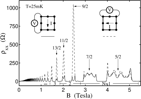
Figure 4.3: Longitudinal resistivity $\rho_{xx}$ in sample A at temperature $T=25$ mK for two perpendicular directions of the current flow through the sample. The two traces result from simply change of the direction of current through the sample; the sample itself is not rotated. The diagrams in the figure depict the difference between two configurations. From Ref. [9].

In this figure, the sample A is a GaAs/AlGaAs heterojunction grown by molecular beam epitaxy, where the density of the sample is close to $n_{s}=2.67\times 10^{11}$ ${\rm cm}^{-2}$, the low temperature mobility is $\mu\geq 9\times 10^{6}{\rm cm}^{2}/Vs$, and the sample size is a $5\times 5$ mm square. The electrical transport measurements have been performed using $2$-$20$ nA, $13$ Hz excitation. For more details about experimental parameters used by Lilly et al. , see Ref. [9]. We refer to these experimental parameters as Lilly’s parameters in this thesis.

In this experiment, longitudinal resistivities $\rho_{xx}$ and Hall resistivities $\rho_{xy}$ have been measured for two different configurations. For the configuration shown in the left inset in Fig. 4.3, $\rho_{xx}$ is almost zero around half-fillings in $l\geq 2$ LLs, such as $\nu=9/2$, $11/2$, $13/2$. On the other hand, for the other configuration shown in the right inset in Fig. 4.3, $\rho_{xx}$ revels very large values around the same fillings, where the sample itself is not rotated and only the direction of current is changed. Here, no quantized plateau in the Hall resistivity $\rho_{xy}$ have been observed around these fillings. These experimental results indicate that the ground state around these fillings is not an isotropic state such as a fractional quantum Hall state but an anisotropic state. Since the original Hamiltonian of the quantum Hall system has a rotational symmetry, it is considered that the anisotropic state is energetically favorable and a spontaneous symmetry breaking occurs with respect to the direction of the anisotropy which would be determined by some small residual inhomogeneity of the sample.

4.3 Highly anisotropic states in the Hartree-Fock theory

In this section, the striped Hall state and the ACDW state at the partial filling factor $\nu^{\ast}=1/2$ in higher LLs are investigated. Calculations are performed by means of a vNL basis within the HF approximation with no injected current. As has been mentioned in Chapter 2, the vNL basis is a suitable basis to study spatially periodic states.

4.3.1 Striped Hall state at $\nu^{\ast}=1/2$

The striped Hall state is obtained as a HF solution under the assumption of the unidirectional charge density wave Eq. (3.1). The solutions at $\nu^{\ast}=1/2$ are given in subsection 3.2.3 in Chapter 3 in detail. Let us consider the striped Hall state in which stripes face the $y$-direction. In this case, the anisotropic Fermi surface of the striped Hall state has the inter-LL energy gap in the $p_{x}$-direction and is gapless in the $p_{y}$-direction. When a current flows in the $y$-direction, an electric field is generated in the $x$-direction owing to the Hall effect so that the Fermi sea slides in the $p_{x}$-direction. Since the Brillouin zone in the $p_{x}$-direction is fully occupied, there is no dissipation in this case and the longitudinal resistivity in the $y$-direction is expected to be zero. On the other hand, when the current flows in the $x$-direction, the Fermi sea slides in the $p_{y}$-direction so that the energy dissipation occurs owing to the gapless structure of the Fermi surface in this direction, which would result in a large longitudinal resistivity. Hence, it is expected that the striped Hall state revels the highly anisotropic longitudinal resistivity, which coincides with the experimental results.

4.3.2 Anisotropic charge density wave state at $\nu^{\ast}=1/2$

CDW states studied in Sec. 3.3 in Chapter 3 become highly anisotropic around $\nu^{\ast}=1/2$ in higher LLs. We call these highly anisotropic states at $\nu^{\ast}=1/2$ “anisotropic charge density wave (ACDW) states” and the direction with a narrower periodicity in density “stripe direction” in this thesis. In the vNL formalism, the HF Hamiltonian of the ACDW state can be rewritten in the form of a $2\times 2$ matrix. Therefore, eigenvalues and eigenstates for the ACDW state can be easily obtained in a more analytical form as a function of order parameters. In what follows, we derive them and discuss the features of the self-consistent ACDW solution.

Let us start by the HF Hamiltonian of the CDW state at $\nu^{\ast}=1/2$. From Eq. (3.15), this is given by

$$\mathcal{H}^{(l)}_{{\rm HF-ACDW}}=\epsilon^{(0)}_{l}N_{e}^{(l)}+\int_{{\rm RBZ}}\frac{d^{2}p}{(2\pi)^{2}}{\bf b}_{l}^{\dagger}({\bf p})D_{l}({\bf p}){\bf b}_{l}({\bf p}),$$ (4.1)

$${\bf b}_{l}({\bf p})=\left(\begin{array}[]{cc}b_{l}(p_{x},p_{y})\\ b_{l}(p_{x},p_{y}+\pi)\end{array}\right),\quad D_{l}({\bf p})=\left(\begin{array}[]{cc}A({\bf p})&B({\bf p})\\ B^{\ast}({\bf p})&A(p_{x},p_{y}+\pi)\end{array}\right),$$ (4.6)

where $\epsilon^{(0)}_{l}$ is a uniform Fock energy given by $\nu^{\ast}v_{l}^{\rm HF}(0)$, the momentum integration is performed over the reduced Brillouin zone (RBZ), $|p_{x}|<\pi$ and $|p_{y}|<\pi/2$, $D_{l}({\bf p})$ is a $2\times 2$ Hermite matrix, and $A({\bf p})$, $B{\bf p}$ are given by

$$A({\bf p})= \sum_{{\bf N}\neq 0}v_{l}^{\rm HF}(\frac{2\pi N_{x}}{r_{s}},2\pi N_{y}r_{s})\Delta_{l}(\frac{2\pi N_{x}}{r_{s}},2\pi N_{y}r_{s})e^{i\pi(N_{x}+N_{y}+N_{x}N_{y})-ip_{x}N_{y}+ip_{y}N_{x}}$$

$$B({\bf p})= \sum_{\bf N}v_{l}^{\rm HF}(\frac{2\pi N_{x}}{r_{s}},\pi(2N_{y}+1)r_{s})\Delta_{l}(\frac{2\pi N_{x}}{r_{s}},\pi(2N_{y}+1)r_{s})e^{i\pi(N_{x}+N_{y}+N_{x}(N_{y}+1/2))-ip_{x}N_{y}+ip_{y}N_{x}}.$$ (4.7)

The Hamiltonian Eq. (4.1) can be diagonalized at each momentum just by unitary transformation of the field operator ${\bf b}_{l}({\bf p})$. In the present case of $\nu^{\ast}=1/2$, the Brillouin zone is reduced to the half size of the original domain and two energy bands are formed (Fig. 4.4).

Figure 4.4: One-particle energy of the $l=2$ ACDW state at half-filling. The uniform Fock energy is subtracted. Two bands are formed and the lower band is completely filled.

$D_{l}({\bf p})$ is diagonalized using the unitary matrix $U({\bf p})$ as

$$U^{\dagger}({\bf p})D_{l}({\bf p})U({\bf p})=\left(\begin{array}[]{cc}\epsilon_{+}({\bf p})&0\\ 0&\epsilon_{-}({\bf p})\end{array}\right).$$ (4.8)

where $\epsilon_{+}({\bf p})$ and $\epsilon_{-}({\bf p})$ represent the upper energy band and the lower energy band respectively. If we assume the $x$- and $y$-inversion symmetries for the density, the order parameters become real and have the property $\Delta_{l}(Q_{x},Q_{y})=\Delta_{l}(Q_{x},-Q_{y})=\Delta_{l}(-Q_{x},Q_{y})$. The self-consistent solution is available only when the two energy bands are symmetric with respect to the energy gap, i.e., $\epsilon_{+}({\bf p})=-\epsilon_{-}({\bf p})\equiv\epsilon({\bf p})$, as expected from the particle-hole symmetry of the original Hamiltonian. This gives ${\rm Tr}_{2\times 2}D_{l}({\bf p})=0$, where ${\rm Tr}_{2\times 2}$ denotes the trace with respect to the $2\times 2$ matrix indices, and $A(p_{x},p_{y}+\pi)=-A({\bf p})$. In this case, $U({\bf p})$ and $\epsilon({\bf p})$ are given by

$$U({\bf p})=\left(\begin{array}[]{cc}\frac{B({\bf p})}{N_{+}({\bf p})}&\frac{B({\bf p})}{N_{-}({\bf p})}\\ \frac{\epsilon_{+}({\bf p})-A({\bf p})}{N_{+}({\bf p})}&\frac{\epsilon_{-}({\bf p})-A({\bf p})}{N_{-}({\bf p})}\end{array}\right),\quad\epsilon({\bf p})=\sqrt{(A({\bf p}))^{2}+|B({\bf p})|^{2}},$$ (4.9)

where $N_{\pm}({\bf p})=2\epsilon_{\pm}({\bf p})(\epsilon_{\pm}({\bf p})-A({\bf p}))$. Using the basis ${\bf c}_{l}({\bf p})=U^{\dagger}({\bf p}){\bf b}_{l}({\bf p})$, we obtain the HF Hamiltonian of the ACDW state

$$\mathcal{H}^{(l)}_{{\rm HF-ACDW}}= \epsilon_{0}N_{e}^{(l)}+\int_{{\rm RBZ}}\frac{d^{2}p}{(2\pi)^{2}}{\bf c}_{l}^{\dagger}({\bf p})\left(\begin{array}[]{cc}\epsilon_{+}({\bf p})&0\\ 0&\epsilon_{-}({\bf p})\end{array}\right){\bf c}_{l}({\bf p}),$$ (4.12)

where

$${\bf c}_{l}({\bf p})=\left(\begin{array}[]{cc}c_{+}(\bf p)\\ c_{-}(\bf p)\end{array}\right),$$ (4.13)

and $\Delta_{l}({\bf Q}_{N})$ is determined as a numerical solution of the self-consistent equation Eq. (3.31).

The HF energy of the ACDW state depends on the asymmetry parameter $r_{s}$. The optimal value of $r_{s}$, the HF energy per particle, and the magnitude of the energy gap are given in Table 4.1,

$l$	$r_{s}^{\rm ACDW}$	$E_{\rm ACDW}/(q^{2}/l_{\rm B})$	$\Delta_{\rm Gap}/(q^{2}/l_{\rm B})$
0	$\sqrt{2}$	-0.4436	0.3292
1	1.02, 1.96	-0.3583	0.3077
2	0.82, 2.44	-0.3097	0.2470
3	0.70, 2.86	-0.2814	0.1967

Table 4.1: Minimum energy and corresponding parameter $r_{s}$ of the ACDW states at $\nu^{\ast}=1/2$. $\Delta_{\rm Gap}$ is a magnitude of the energy gap.

in which there are two values of $r_{s}$ at each LL owing to the $\pi/2$-rotational symmetry. The magnitude of the energy gap is estimated to be of the order of $10$ K for a few tesla. Therefore, the extremely anisotropic longitudinal resistivities are not expected at tens of milli Kelvin and it is difficult to explain the experiments with the ACDW state. On the other hand, the HF energy of the ACDW state is slightly lower than that of the striped Hall state at each LL. This was one of the remaining issues for the anisotropic states.

4.4 Response functions

In this section, electromagnetic response functions of the two HF states are calculated in the long wavelength limit. We consider the quantum Hall system with an infinitesimal external gauge field $a_{\mu}(x)=(a_{0}(x),-{\bm{a}}(x))$ and calculate the response functions of the striped Hall state and the ACDW state. These response functions will be used to determine current and charge distributions and energy corrections due to an injected current in Sec. 4.5.

4.4.1 Response function of the striped Hall state

The Hamiltonian in the quantum Hall system with $a_{\mu}(x)$ is given by

$$H= \int d^{2}x\Psi^{\dagger}({\bf x})\left(\frac{(-i\nabla+e{\bf A}({\bf x})+e{\bm{a}}({\bf x}))^{2}}{2m_{e}}-ea_{0}({\bf x})\right)\Psi({\bf x})+\frac{1}{2}\int d^{2}xd^{2}x^{\prime}:\rho({\bf x})V({\bf x}-{\bf x}^{\prime})\rho({\bf x}^{\prime}):,$$ (4.14)

where $V({\bf x})=q^{2}/|{\bf x}|$. We project the Coulomb interaction part to each LL and apply the HF approximation to the projected Coulomb interaction. Then, by using the vNL basis, the Hamiltonian in the HF approximation is given by

$$H= \sum_{l}E_{l}\int_{\rm BZ}\frac{d^{2}p}{(2\pi)^{2}}b_{l}^{\dagger}({\bf p})b_{l}({\bf p})$$

$$-\int\frac{d^{2}k}{(2\pi)^{2}}\sum_{l,l^{\prime}}ef^{\mu}_{l,l^{\prime}}(\tilde{\bf k})a_{\mu}(\tilde{\bf k})\int_{\rm BZ}\frac{d^{2}p}{(2\pi)^{2}}b^{\dagger}_{l}({\bf p})b_{l^{\prime}}({\bf p}-{\bf k})e^{-(i/4\pi)k_{x}(2p_{y}-k_{y})}$$

$$+\int\frac{d^{2}kd^{2}k^{\prime}}{(2\pi)^{4}}\sum_{l,l^{\prime}}\frac{e^{2}\omega_{c}}{4\pi}{\bm{a}}(\tilde{\bf k})\cdot{\bm{a}}(\tilde{\bf k}^{\prime})f^{0}_{l,l^{\prime}}(\tilde{\bf k}+\tilde{\bf k}^{\prime})\int_{\rm BZ}\frac{d^{2}p}{(2\pi)^{2}}b^{\dagger}_{l}({\bf p})b_{l^{\prime}}({\bf p}-{\bf k}-{\bf k}^{\prime})e^{-(i/4\pi)(k_{x}+k^{\prime}_{x})(2p_{y}-k_{y}-k^{\prime}_{y})}$$

$$+\sum_{l}\int\frac{d^{2}k}{(2\pi)^{2}}v_{l}^{\rm HF}({\bf k})\langle\bar{\rho}_{l}(-\tilde{\bf k})\rangle\bar{\rho}_{l}(\tilde{\bf k}),$$ (4.15)

where $f^{\mu}_{l_{1},l_{2}}({\bf k})$ is defined by (see Appendix A.4)

$$f^{\mu}_{l_{1},l_{2}}({\bf k})=\langle f_{l_{1}}|\frac{1}{2}\{v^{\mu},e^{i{\bf k}\cdot{\bm{\xi}}}\}|f_{l_{2}}\rangle$$ (4.16)

in which $v^{\mu}=(1,-\omega_{c}\eta,\omega_{c}\xi)$ is the electron velocity. Repeated Greek indices $\mu$ and $\nu$ are summed for 0, 1, 2 in throughout the following calculations. The action is given by

$$S[a_{\mu},b,b^{\dagger}]=\int dt\Big{[} \int_{\rm BZ}\frac{d^{2}p}{(2\pi)^{2}}b^{\dagger}_{l}({\bf p},t)(i\partial_{t}+\mu_{\rm F})b_{l}({\bf p},t)-H(t)\Big{]},$$ (4.17)

where $H(t)$ is the Heisenberg representation of $H$.

Let us concentrate on the striped Hall state with the stripe direction facing the $y$-direction at half-filling. Substituting Eq. (3.3) into Eq. (4.17), we obtain the action of the striped Hall state given by

$$S_{\rm HF}[a_{\mu},b,b^{\dagger}]=\sum_{l,l^{\prime}}\int_{\rm BZ}\frac{d^{3}pd^{3}p^{\prime}}{(2\pi)^{6}}b_{l}^{\dagger}(p)\Bigl{[}(p_{0}-\xi_{l}({\bf p}))\delta_{l,l^{\prime}}(2\pi)^{3}\delta^{3}(p-p^{\prime})-U_{a_{1}}^{(l,l^{\prime})}(p,p^{\prime})-U_{a_{2}}^{(l,l^{\prime})}(p,p^{\prime})\Bigr{]}b_{l^{\prime}}(p^{\prime}),$$ (4.18)

where

$$U_{a_{1}}^{(l,l^{\prime})}(p,p^{\prime})= -\sum_{\bf N}ef^{\mu}_{l,l^{\prime}}(\tilde{\bf p}-\tilde{\bf p}^{\prime}-2\pi\tilde{\bf N})h({\bf p}+{\bf p}^{\prime},{\bf N})a_{\mu}(p_{0}-p^{\prime}_{0},\tilde{\bf p}-\tilde{\bf p}^{\prime}-2\pi\tilde{\bf N})e^{-(i/4\pi)(p_{x}-p^{\prime}_{x})(p_{y}+p^{\prime}_{y})},$$

$$U_{a_{2}}^{(l,l^{\prime})}(p,p^{\prime})= \sum_{\bf N}\int\frac{d^{3}k}{(2\pi)^{3}}\frac{e^{2}\omega_{c}}{4\pi}f^{0}_{l,l^{\prime}}(\tilde{\bf p}-\tilde{\bf p}^{\prime}-2\pi\tilde{\bf N})h({\bf p}+{\bf p}^{\prime},{\bf N})$$

$$\times{\bm{a}}(k_{0},\tilde{\bf k})\cdot{\bm{a}}(p_{0}-p^{\prime}_{0}-k_{0},\tilde{\bf p}-\tilde{\bf p}^{\prime}-\tilde{\bf k}-2\pi\tilde{{\bf N}})e^{-(i/4\pi)(p_{x}-p^{\prime}_{x})(p_{y}+p^{\prime}_{y})}$$

$$h({\bf p},{\bf N})\equiv(-1)^{N_{x}+N_{y}+N_{x}N_{y}}e^{-(i/2)p_{x}N_{y}+(i/2)p_{y}N_{x}}.$$ (4.19)

Here, $p$ denotes $(p_{0},{\bf p})$, $\xi_{l}({\bf p})=E_{l}+\epsilon_{l}({\bf p})-\epsilon_{\rm F}$, and $U_{a_{1}}^{(l,l^{\prime})}(p,p^{\prime})$ and $U_{a_{2}}^{(l,l^{\prime})}(p,p^{\prime})$ are the first order term and the second order term with respect to $a_{\mu}(p)$, respectively.

The partition function $Z[a]$ is calculated using path integrals by

$$Z[a_{\mu}]= \int\mathcal{D}b^{\dagger}\mathcal{D}b\,e^{iS_{\rm HF}[a_{\mu},b,b^{\dagger}]}$$

$$= \int\mathcal{D}b^{\dagger}\mathcal{D}b\,e^{-(-i)\sum b^{\dagger}(g^{-1}{\bf 1}-U_{a_{1}}-U_{a_{2}})b}=e^{{\rm Tr}\log[(-i)g^{-1}]}e^{{\rm Tr}\log[{\bf 1}-gU_{a_{1}}-gU_{a_{2}}]},$$ (4.20)

where the power of the exponent is expressed in the matrix representation in momentum space and ${\rm Tr}$ denotes the trace of the momentum indices and the LL indices. $g_{l}(p)$ is the Green function given by

$$g_{l}(p)=\frac{\theta(\xi_{l}({\bf p}))}{p_{0}-\xi_{l}({\bf p})+i\delta}+\frac{\theta(-\xi_{l}({\bf p}))}{p_{0}-\xi_{l}({\bf p})-i\delta},$$ (4.21)

where $\delta$ is an infinitesimal positive constant. The effective action $S_{\rm eff}[a_{\mu}]$ is defined as $S_{\rm eff}[a_{\mu}]=-i\log Z[a_{\mu}]$, which consists of the non-perturbed part $S_{0}={\rm Tr}\log[(-i)g^{-1}]$ and the correction part due to the external gauge field $\Delta S_{\rm eff}[a_{\mu}]$. $\Delta S_{\rm eff}[a_{\mu}]$ is given by (Fig. 4.5),

$$\Delta S_{\rm eff}[a_{\mu}]=\Delta S_{1}[a_{\mu}]+\Delta S_{2}[a_{\mu}]+\Delta S_{3}[a_{\mu}]+\mathcal{O}[a_{\mu}^{3}],$$ (4.22)

where

$$\Delta S_{1}[a_{\mu}]= i{\rm Tr}[gU_{a_{1}}]=i\sum_{l}\int_{\rm BZ}\frac{d^{3}p}{(2\pi)^{3}}g_{l}(p)U^{(l,l)}_{a_{1}}(p,p),$$

$$\Delta S_{2}[a_{\mu}]= i{\rm Tr}[gU_{a_{2}}]=i\sum_{l}\int_{\rm BZ}\frac{d^{3}p}{(2\pi)^{3}}g_{l}(p)U^{(l,l)}_{a_{2}}(p,p),$$

$$\Delta S_{3}[a_{\mu}]= \frac{i}{2}{\rm Tr}[gU_{a_{1}}gU_{a_{1}}]=\frac{i}{2}\sum_{l,l^{\prime}}\int_{\rm BZ}\frac{d^{3}pd^{3}p^{\prime}}{(2\pi)^{6}}g_{l}(p)U^{(l,l^{\prime})}_{a_{1}}(p,p^{\prime})g_{l^{\prime}}(p^{\prime})U^{(l^{\prime},l)}_{a_{1}}(p^{\prime},p).$$ (4.23)

Figure 4.5: (a), (b) and (c) are Feynman diagrams for $\Delta S_{1}$, $\Delta S_{2}$ and $\Delta S_{3}$, respectively.

Substituting the expressions for $g_{l}(p)$, $U_{a1}^{(l,l^{\prime})}(p,p^{\prime})$ and $U_{a2}^{(l,l^{\prime})}(p,p^{\prime})$ into Eq. (4.23), we obtain

$$\Delta S_{\rm eff}[a_{\mu}]= (el_{0})a_{0}(0,{\bf 0})+\sum_{N_{x}}ef^{\mu}_{l_{0},l_{0}}(-2\pi N_{x}/r_{s},0)\frac{\sin(p_{F}N_{x})}{\pi N_{x}}e^{i\pi N_{x}}a_{\mu}(0,-2\pi N_{x}/r_{s},0)$$

$$-\frac{1}{2}\int\frac{d^{3}p}{(2\pi)^{3}}\sum_{\bf N}a_{\mu}(p_{0},{\bf p})K^{\mu\nu}(p,{\bf N})a_{\nu}(-p_{0},-{\bf p}-2\pi\tilde{\bf N}),$$ (4.24)

where $l_{0}$ represents the uppermost partially filled LL and $\tilde{\bf N}=(N_{x}/r_{s},r_{s}N_{y})$. $K^{\mu\nu}(p,{\bf N})$ is a response function given by

$$K^{\mu\nu}(p,{\bf N})= \sum_{l,l^{\prime}}e^{2}f^{\mu}_{l,l^{\prime}}({\bf p})f^{\nu}_{l^{\prime},l}(-{\bf p}-2\pi\tilde{\bf N})I_{l,l^{\prime}}(p_{0},\hat{\bf p},{\bf N})h(\hat{\bf p},{\bf N})$$

$$+\frac{e^{2}}{2\pi}\omega_{c}\sum_{\bf N}\left[l_{0}\delta_{{\bf N},0}+f_{l_{0},l_{0}}^{0}(-2\pi\tilde{\bf N})(-1)^{N_{x}}\frac{\sin(\pi N_{x}/2)}{\pi N_{x}}\delta_{N_{y},0}\right](\delta_{\mu,1}\delta_{\nu,1}+\delta_{\mu,2}\delta_{\nu,2}),$$ (4.25)

and $I_{l,l^{\prime}}(p_{0},{\bf p},{\bf N})$ is the loop integral in Fig. 4.5 (c), which is given by

$$I_{l,l^{\prime}}(p_{0},{\bf p},{\bf N})= \int_{\rm BZ}\frac{d^{2}p^{\prime}}{(2\pi)^{2}}\Biggl{[}\frac{\theta(\xi_{l}({\bf p}+{\bf p}^{\prime}))\theta(-\xi_{l^{\prime}}({\bf p}^{\prime}))}{p_{0}+\xi_{l^{\prime}}({\bf p}^{\prime})-\xi_{l}({\bf p}+{\bf p}^{\prime})+i\delta}-\frac{\theta(-\xi_{l}({\bf p}+{\bf p}^{\prime}))\theta(\xi_{l^{\prime}}({\bf p}^{\prime}))}{p_{0}+\xi_{l^{\prime}}({\bf p}^{\prime})-\xi_{l}({\bf p}+{\bf p}^{\prime})-i\delta}\Biggr{]}e^{-ip^{\prime}_{x}N_{y}+ip^{\prime}_{y}N_{x}},$$ (4.26)

in which the $p^{\prime}_{0}$ integral has been performed. In Eq. (4.4.1), the first term and the second term come from $\Delta S_{3}[a_{\mu}]$ and $\Delta S_{2}[a_{\mu}]$, respectively, and the second term is canceled with the $p=0$ part of the first term, as expected from gauge invariance. Hence, $K^{i,i}(p=0,{\bf N})=0$ for $i=1,2$.

In the long wavelength limit, the largest contribution in the response function comes from the ${\bf N}=0$ part. In the case of $p_{0}=p_{y}=0$ and $p_{x}\to 0$, which is used in the next section, the largest contribution comes from the lowest order term in $K^{\mu\nu}_{0}(p_{x})\equiv K^{\mu\nu}(0,p_{x},0)$ with respect to $p_{x}$. Expanding $K^{\mu\nu}_{0}(p_{x})$ up to the lowest order, we obtain the response functions in the long wavelength limit given by

$$K^{00}_{0}(p_{x})= -\frac{\sigma^{(\nu)}_{xy}}{\omega_{c}}p^{2}_{x},\qquad K^{0y}_{0}(p_{x})=-i\sigma^{(\nu)}_{xy}p_{x},$$

$$K^{y0}_{0}(p_{x})= i\sigma^{(\nu)}_{xy}p_{x},\qquad K^{yy}_{0}(p_{x})=\alpha_{K}\omega_{c}p^{2}_{x},$$ (4.27)

where $\sigma^{(\nu)}_{xy}=e^{2}\nu/2\pi$ and $\alpha_{K}=e^{2}\omega_{c}(l_{0}^{2}+2l_{0}\nu^{\ast}+\nu^{\ast})/4\pi^{2}$. $\sigma_{xy}^{(\nu)}$ is identified as the Hall conductance since if we consider a static homogeneous electric field in the $x$-direction generated by the gauge field $a_{0}^{\rm ex}(x)=xE_{x}$, then the electric current in the $y$-direction $\langle j_{y}(x)\rangle$ is given in the long wavelength limit by $\langle j_{y}(x)\rangle=\delta\Delta S_{\rm eff}/\delta a_{y}(x)=K^{y0}_{0}(\partial_{x})a_{0}(x)=-\sigma_{xy}^{(\nu)}E_{x}$, where the response function transformed in the coordinate space is used. The longitudinal resistivity becomes zero in the present calculation since the impurity potential is not included. If impurities are added, it is expected that the longitudinal resistivity becomes zero in one direction and finite in the other direction owing to the anisotropic Fermi surface.

4.4.2 Response function of the anisotropic charge density wave state

The action of the ACDW state at half-filling is given by

$$S_{\rm HF}[a_{\mu},{\bf c},{\bf c}^{\dagger}]=\sum_{l,l^{\prime}}\int_{\rm RBZ}\frac{d^{3}pd^{3}p^{\prime}}{(2\pi)^{6}}{\bf c}_{l}^{\dagger}(p)\Big{[}G^{-1}_{l}(p)\delta_{l,l^{\prime}}(2\pi)^{3}\delta^{3}(p-p^{\prime})-V^{(l,l^{\prime})}_{a_{1}}(p;p^{\prime})-V^{(l,l^{\prime})}_{a_{2}}(p;p^{\prime})\Big{]}{\bf c}_{l^{\prime}}(p^{\prime}),$$ (4.28)

where $V_{a_{j}}^{(l,l^{\prime})}(p;p^{\prime})$ with $j=1,2$ is a $2\times 2$ matrix given by

$$V_{a_{j}}^{(l,l^{\prime})}(p;p^{\prime})= U^{{\dagger}}({\bf p}){\bf U}^{(l,l^{\prime})}_{a_{j}}(p;p^{\prime})U({\bf p}),$$

$${\bf U}_{a_{j}}^{(l,l^{\prime})}(p;p^{\prime})= \left(\begin{array}[]{cc}U_{a_{j}}^{(l,l^{\prime})}(p;p^{\prime})&U_{a_{j}}^{(l,l^{\prime})}(p;p^{\prime}_{0},p^{\prime}_{x},p^{\prime}_{y}+\pi)\\ U_{a_{j}}^{(l,l^{\prime})}(p_{0},p_{x},p_{y}+\pi;p^{\prime})&U_{a_{j}}^{(l,l^{\prime})}(p_{0},p_{x},p_{y}+\pi;p^{\prime}_{0},p^{\prime}_{x},p^{\prime}_{y}+\pi)\end{array}\right),$$ (4.31)

and $G_{l}(p)$ is a $2\times 2$ matrix Green function given by

$$G_{l}(p)=\left\{\begin{array}[]{ll}\left(\begin{array}[]{cc}g^{+}_{l}(p)&0\\ 0&g^{-}_{l}(p)\end{array}\right)&{\rm for}\quad l=l_{0}\\ g^{-}_{l}(p){\bf 1}&{\rm for}\quad l<l_{0}\\ g^{+}_{l}(p){\bf 1}&{\rm for}\quad l>l_{0}\end{array}\right..$$ (4.32)

In Eq. (4.32), $g^{\pm}_{l}(p)=1/(p_{0}-\xi^{\pm}_{l}(p)\pm i\delta)$ is a one-particle Green function for the upper or lower band, ${\bf 1}$ is a $2\times 2$ unit matrix, and $\xi^{\pm}_{l}({\bf p})=E_{l_{0}}+\epsilon^{(l_{0})}_{\pm}({\bf p})-\epsilon_{\rm F}$.

The partition function $Z[a_{\mu}]$ is calculated using path integrals by

$$Z[a_{\mu}]=\int\mathcal{D}{\bf c}^{\dagger}\mathcal{D}{\bf c}\,e^{iS_{\rm HF}[a_{\mu},{\bf c},{\bf c}^{\dagger}]}=e^{{\rm Tr}\log[(-i)G^{-1}]}e^{{\rm Tr}\log[{\bf 1}-GV_{a_{1}}-GV_{a_{2}}]}.$$ (4.33)

The correction part of the effective action $\Delta S_{\rm eff}[a_{\mu}]$ is given by

$$\Delta S_{\rm eff}[a_{\mu}]=\Delta S_{1}[a_{\mu}]+\Delta S_{2}[a_{\mu}]+\Delta S_{3}[a_{\mu}]+\mathcal{O}[a_{\mu}^{3}],$$ (4.34)

where

$$\Delta S_{1}[a_{\mu}]= i{\rm Tr}[GV_{a_{1}}]=i\sum_{l}\int_{\rm RBZ}\frac{d^{3}p}{(2\pi)^{3}}{\rm Tr_{2\times 2}}[G_{l}(p)V^{(l,l)}_{a_{1}}(p;p)],$$

$$\Delta S_{2}[a_{\mu}]= i{\rm Tr}[GV_{a_{2}}]=i\sum_{l}\int_{\rm RBZ}\frac{d^{3}p}{(2\pi)^{3}}{\rm Tr_{2\times 2}}[G_{l}(p)V^{(l,l)}_{a_{2}}(p;p)],$$

$$\Delta S_{3}[a_{\mu}]= \frac{i}{2}{\rm Tr}[GV_{a_{1}}GV_{a_{1}}]=\frac{i}{2}\sum_{l,l^{\prime}}\int_{\rm RBZ}\frac{d^{3}pd^{3}p^{\prime}}{(2\pi)^{6}}{\rm Tr_{2\times 2}}[G_{l}(p)V^{(l,l^{\prime})}_{a_{1}}(p;p^{\prime})G_{l^{\prime}}(p^{\prime})V^{(l^{\prime},l)}_{a_{1}}(p^{\prime};p)].$$ (4.35)

Here, ${\rm Tr}$ denotes the trace with respect to the momentum indices, the LL indices and the $2\times 2$ matrix indices, and ${\rm Tr}_{2\times 2}$ denotes the trace with respect to only the $2\times 2$ matrix indices. Substituting the expressions for $G_{l}(p)$, $V_{a_{1}}^{(l,l^{\prime})}(p;p^{\prime})$, $V_{a_{2}}^{(l,l^{\prime})}(p;p^{\prime})$ into Eq. (4.35), we obtain the following expression for the ${\bf N}=0$ part of $\Delta S_{\rm eff}[a_{\mu}]$ as in the case of the striped Hall state,

$$\Delta S_{\rm eff}[a_{\mu}]= e(l_{0}+\frac{1}{2})a_{0}(0,{\bf 0})-\frac{1}{2}\int\frac{d^{3}p}{(2\pi)^{3}}a_{\mu}(p_{0},{\bf p})K_{0}^{\mu\nu}(p)a_{\nu}(-p_{0},-{\bf p}),$$ (4.36)

where $K^{\mu\nu}_{0}(p)$ is given by

$$K^{\mu\nu}_{0}(p)= -\sum_{l<l_{0}}\sum_{l^{\prime}>l_{0}}\frac{e^{2}}{\omega_{c}(l^{\prime}-l)}\left\{f^{\mu}_{l,l^{\prime}}({\bf p})f^{\nu}_{l^{\prime},l}(-{\bf p})+f^{\mu}_{l^{\prime},l}({\bf p})f^{\nu}_{l,l^{\prime}}(-{\bf p}))\right\}$$

$$+\frac{1}{2}\left[-\sum_{l<l_{0}}+\sum_{l>l_{0}}\right]\frac{e^{2}}{\omega_{c}(l_{0}-l)}\left\{f^{\mu}_{l,l_{0}}({\bf p})f^{\nu}_{l_{0},l}(-{\bf p})+f^{\mu}_{l_{0},l}({\bf p})f^{\nu}_{l,l_{0}}(-{\bf p})\right\}$$

$$+\int_{\rm RBZ}\frac{d^{2}p^{\prime}}{(2\pi)^{2}}\frac{1}{p_{0}-(\epsilon({\bf p}^{\prime})+\epsilon(\hat{\bf p}+{\bf p}^{\prime}))}$$

$$\qquad\times\left[1-\frac{A(\hat{\bf p}+{\bf p}^{\prime})A({\bf p}^{\prime})+{\rm Re}(B(\hat{\bf p}+{\bf p}^{\prime})B^{\ast}({\bf p}^{\prime})e^{-(i/2)r_{s}p_{x}})}{\epsilon(\hat{\bf p}+{\bf p}^{\prime})\epsilon({\bf p}^{\prime})}\right]e^{2}f^{\mu}_{l_{0},l_{0}}({\bf p})f^{\nu}_{l_{0},l_{0}}(-{\bf p})$$

$$+(l_{0}+\frac{1}{2})\frac{e^{2}}{2\pi}\omega_{c}(\delta_{\mu,1}\delta_{\nu,1}+\delta_{\mu,2}\delta_{\nu,2}),$$ (4.37)

up to $\mathcal{O}(\epsilon({\bf p})/\omega_{C})$. In Eq. (4.4.2), the last term is canceled with the $p=0$ term of the second term as expected from gauge invariance again. Hence, $K_{0}^{i,i}(0)=0$ for $i=1,2$.

In the long wavelength limit $p_{0}=p_{y}=0$ and $p_{x}\to 0$, the largest contribution in the response function comes from the lowest order term with respect to $p_{x}$. The expressions of $K_{0}^{0y}(p_{x})$ and $K_{0}^{y0}(p_{x})$ become the same as in the case of the striped Hall state. The expression of $K_{0}^{00}(p_{x})$ becomes slightly different by the correction from the intra-LL effect at the uppermost partially-filled LL. For the striped Hall state, the one-particle energy shown in Fig. 3.3 has the inter-LL energy gap in the $p_{x}$-direction, and the inter-LL effect gives the response functions given in Eq. (4.4.1). For the ACDW state, the one-particle energy shown in Fig. 4.4 has the intra-LL energy gap in the $p_{x}$-direction as well as the inter-LL energy gap. While the inter-LL effect gives the same expression of the response function as that of the striped Hall state, the intra-LL effect causes some corrections to the response function. Including these corrections, we obtain $K_{0}^{00}(p_{x})$ of the ACDW state in the long wavelength limit given by (see Appendix B.2)

$$K^{00}_{0}(p_{x})=-(1+\frac{\sqrt{B}}{\nu}\beta)\frac{\sigma_{xy}^{(\nu)}}{\omega_{c}}p_{x}^{2},$$ (4.38)

where $a=\sqrt{2\pi/eB}$ is used explicitly in order to compare the theoretical results with experimental data. The value of $\beta$ at each LL is shown in Table 4.2. Note that the unit of $\beta$ is $({\rm tesla})^{-1/2}$.

$l$	parallel	perpendicular
0	0.497	0.497
1	0.386	0.824
2	0.472	1.044
3	0.581	1.171

Table 4.2: The value of $\beta$ at each LL. parallel is the case in which the stripe direction faces the $y$-direction. perpendicular is the case in which the stripe direction faces the $x$-direction. The unit of $\beta$ is $({\rm tesla})^{-1/2}$.

The Hall conductance is given by $\sigma_{xy}^{(\nu)}=e^{2}\nu/2\pi$, as in the case of the striped Hall state. The longitudinal resistivity becomes zero in the present calculation since the impurity potential is not included. However it is expected that the longitudinal resistivity remains zero even in the system with impurities because of the energy gaps.

4.5 Energy corrections due to injected currents

In this section, we consider the quantum Hall system with an injected electric current and investigate the current effect on the striped Hall state and the ACDW state. Effects of impurities and metallic contacts are ignored in our calculations. For the striped Hall state, we only consider the current parallel to the stripe direction since in this case, the current effect can be estimated with no ambiguity even in the system with impurities. When the current flows in the stripe direction, charges accumulate around both edges of the sample in the direction perpendicular to the stripe direction (perpendicular direction), as we will see later, and the electric field generates in the perpendicular direction. In this case, the impurity effect is negligible since the Fermi surface has the inter-LL energy gap in the perpendicular direction. On the other hand, when the current flows in the perpendicular direction, the impurity effect becomes relevant since the electric field generates in the stripe direction while the Fermi surface is gapless in this direction. The current effect in this case is nontrivial and will be studied in future work.

In the system with an injected current, it is naively expected that the current flow causes the plus and minus charge accumulation at both edges of the sample with the opposite sign, as expected from the classical Hall effect. MacDonald et al. have studied effects of an injected current on the integer quantum Hall state about two decades ago [50]. They have calculated current and charge distributions and found that the charge accumulation occurs in the integer quantum Hall state. The charge accumulation causes the energy correction via the Coulomb interaction between the accumulated charges. It is expected that the same type of energy corrections exists even in the present highly correlated quantum Hall states. However, it has not been studied as far as the present authors know. In what follows, first, we derive current and charge distributions in the striped Hall state and the ACDW state using the effective action, then, we estimate the current dependence of energy corrections of the two HF states. It is shown that the energy of the ACDW state increases faster than that of the striped Hall state as the injected current increases.

4.5.1 Current and charge distributions

We study current and charge distributions of the striped Hall state and the ACDW state. Let us begin with the system with no injected current. We denote the two-point function in the HF theory with no injected current as $\langle\Psi^{\dagger}({\bf x},t)\Psi({\bf x}^{\prime},t)\rangle_{I=0}$. If a finite electric current is injected, electromagnetic fields and the two-point function deviate from their original values. We define these deviations by

$${\bm{a}}({\bf x},t)= {\bf A}({\bf x},t)-{\bf A}_{\rm ex}({\bf x}),$$

$$\delta\rho({\bf x},{\bf x}^{\prime},t)= \langle\Psi^{\dagger}({\bf x},t)\Psi({\bf x}^{\prime},t)\rangle-\langle\Psi^{\dagger}({\bf x},t)\Psi({\bf x}^{\prime},t)\rangle_{I=0},$$ (4.39)

where ${\bm{a}}({\bf x},t)$ and $\delta\rho({\bf x},{\bf x}^{\prime},t)$ are unspecified for the moment and will be determined later. The total action in the Coulomb gauge $\nabla\cdot{\bf A}(x)=0$ is given as

$$S_{\rm tot}[{\bf A},\Psi^{\dagger},\Psi]= \int dtd^{3}x\left(\frac{\epsilon}{2}{\dot{\bf A}}^{2}({\bf x},t)-\frac{1}{2\mu}(\nabla\times{\bf A}({\bf x},t))^{2}\right)$$

$$+\int dtd^{3}x\Psi^{\dagger}({\bf x},t)\left(i\partial_{t}-\frac{({\bf p}+e{\bf A}({\bf x},t))^{2}}{2m^{\ast}}\right)\Psi({\bf x},t)\delta(z)$$

$$-\frac{1}{2}\int dtd^{3}xd^{3}x^{\prime}\Psi^{\dagger}({\bf x},t)\Psi^{\dagger}({\bf x}^{\prime},t)V({\bf x}-{\bf x}^{\prime})\Psi({\bf x}^{\prime},t)\Psi({\bf x},t)\delta(z)\delta(z^{\prime}).$$ (4.40)

where $\mu$ is the magnetic constant, $m^{\ast}$ is the effective electron mass, and the dot means the time derivative. This total action consists of the three-dimensional electromagnetic field term and the two-dimensional electron field term. In the Coulomb gauge, the interaction between electric fields is expressed by the Coulomb interaction. By applying the HF approximation to the Coulomb interaction part and substituting Eq. (4.5.1) into Eq. (4.40), we rewrite the total action as

$$S_{\rm tot}[\delta\rho,{\bm{a}},\Psi^{\dagger},\Psi]=S_{\rm EM}[{\bm{a}}]+S_{\rm HF}[\delta\rho,{\bm{a}},\Psi^{\dagger},\Psi],$$ (4.41)

where

$$S_{\rm EM}[{\bm{a}}]= \int dtd^{3}x\left(\frac{\epsilon}{2}\dot{{\bm{a}}}^{2}({\bf x},t)-\frac{1}{2\mu}(\nabla\times{\bm{a}}({\bf x},t))^{2}\right),$$

$$S_{\rm HF}[\delta\rho,{\bm{a}},\Psi^{\dagger},\Psi]= \int dtd^{3}x\Psi^{\dagger}({\bf x},t)\left(i\partial_{t}-\frac{({\bf p}+e{\bf A}_{\rm ex}({\bf x})+e{\bm{a}}({\bf x},t))^{2}}{2m^{\ast}}\right)\Psi({\bf x},t)\delta(z)$$

$$-\int dtd^{3}xd^{3}x^{\prime}\Big{[}(\langle\Psi^{\dagger}({\bf x},t)\Psi({\bf x},t)\rangle_{I=0}+\delta\rho({\bf x},{\bf x},t))V({\bf x}-{\bf x^{\prime}})\Psi^{\dagger}({\bf x}^{\prime},t)\Psi({\bf x}^{\prime},t)$$

$$-(\langle\Psi^{\dagger}({\bf x},t)\Psi({\bf x}^{\prime},t)\rangle_{I=0}+\delta\rho({\bf x},{\bf x}^{\prime},t))V({\bf x}-{\bf x^{\prime}})\Psi^{\dagger}({\bf x}^{\prime},t)\Psi({\bf x},t)\Big{]}\delta(z)\delta(z^{\prime}).$$ (4.42)

In the expression of $S_{\rm EM}[{\bm{a}}]$, the term of the uniform external magnetic field is dropped since it gives only the same energy constant to the two HF states. In Eq. (4.42), the term including $\delta\rho({\bf x,}{\bf x},t)$ and the term including $\delta\rho({\bf x},{\bf x}^{\prime},t)$ are the Hartree term and the Fock term, respectively. As seen in Appendix B.1, the Fock term becomes negligible compared to the Hartree term in the long wavelength limit since in the momentum space, the Hartree term is proportional to the Coulomb potential $V({\bf k})$, which is $\mathcal{O}(1/k)$, and gives a larger contribution than the Fock term for the small momentum $k$. In the following calculation, the deviation of the Fock term is dropped. If we introduce the potential generated by the electron density deviation as

$$a_{0}({\bf x},t)\equiv\int d^{3}x^{\prime}\frac{(-e)\delta\rho({\bf x}^{\prime},{\bf x}^{\prime},t)}{4\pi\epsilon|{\bf x}-{\bf x}^{\prime}|}\delta(z^{\prime}).$$ (4.43)

$S_{\rm HF}$ is rewritten as

$$S_{\rm HF}[a_{0},{\bm{a}},\Psi^{\dagger},\Psi]= \int dtd^{3}x\Psi^{\dagger}({\bf x},t)\left(i\partial_{t}+ea_{0}({\bf x},t)-\frac{({\bf p}+e{\bf A}_{\rm ex}({\bf x})+e{\bm{a}}({\bf x},t))^{2}}{2m^{\ast}}\right)\Psi({\bf x},t)\delta(z)$$

$$-\int dtd^{3}xd^{3}x^{\prime}\Big{[}\langle\Psi^{\dagger}({\bf x},t)\Psi({\bf x},t)\rangle_{I=0}V({\bf x}-{\bf x^{\prime}})\Psi^{\dagger}({\bf x}^{\prime},t)\Psi({\bf x}^{\prime},t)$$

$$\qquad-\langle\Psi^{\dagger}({\bf x},t)\Psi({\bf x}^{\prime},t)\rangle_{I=0}V({\bf x}-{\bf x^{\prime}})\Psi^{\dagger}({\bf x}^{\prime},t)\Psi({\bf x},t)\Big{]}\delta(z)\delta(z^{\prime}).$$ (4.44)

This HF action $S_{\rm HF}$ has the same form as the Hamiltonian in the system with the infinitesimal external gauge field shown in Eq. (4.14) if we apply the HF approximation to the Coulomb interaction part. The important difference is that $a_{\mu}({\bf x},t)$ in the present case represents not the infinitesimal external gauge field but the finite gauge field induced by the current flow. Although the meaning of $a_{\mu}({\bf x},t)$ is different, the effective action obtained in the previous section is applicable as long as $a_{\mu}({\bf x},t)$ is small.

The partition function is given by

$$Z=\int{\mathcal{D}}{\bm{a}}\int{\mathcal{D}}\Psi^{\dagger}{\mathcal{D}}\Psi\,e^{iS_{\rm EM}[{\bm{a}}]+iS_{\rm HF}[a_{0},{\bm{a}},\Psi^{\dagger},\Psi]}.$$ (4.45)

Integrating out electron fields and expanding the results up to second order of $a_{0}({\bf x},t)$ and ${\bm{a}}({\bf x},t)$, we obtain the effective action $S_{\rm eff}[a_{0},{\bm{a}}]$ as

$$Z=\int{\mathcal{D}}{\bm{a}}\,e^{iS_{\rm EM}[{\bm{a}}]+iS_{0}+i\Delta S_{\rm eff}[a_{0},{\bm{a}}]}.$$ (4.46)

The functional derivative of $(S_{\rm EM}[{\bm{a}}]+S_{0}+\Delta S_{\rm eff}[a_{0},{\bm{a}}])$ with respect to ${\bm{a}}({\bf x},t)$ gives the Maxwell’s equation for ${\bm{a}}({\bf x},t)$,

$$(\epsilon\partial^{2}_{t}-\frac{1}{\mu}\nabla^{2}){\bm{a}}({\bf x},t)=\langle{\bf j}({\bf x},t)\rangle_{a}\delta(z),$$ (4.47)

where ${\bf j}({\bf x},t)$ is a current operator and $\langle\hat{O}(x)\rangle_{a}$ means an expectation value of an operator $\hat{O}(x)$ for the system with finite $a_{\mu}({\bf x},t)$ (or equivalently finite currents). The solution of this equation gives the stationary point of the action with respect to $a_{\mu}({\bf x},t)$. We use the action into which the solution of Eq. (4.47) is substituted as the effective action. $\langle{\bf j}({\bf x},t)\rangle_{a}$ and $\delta\rho({\bf x},t)\equiv\delta\rho({\bf x},{\bf x},t)$ are calculated from the effective action by

$$\frac{\delta\Delta S_{\rm eff}[a_{0},{\bm{a}}]}{\delta{\bm{a}}({\bf x},t)}= \langle{\bf j}({\bf x},t)\rangle_{a}\delta(z),$$

$$-\frac{\delta\Delta S_{\rm eff}[a_{0},{\bm{a}}]}{\delta a_{0}({\bf x},t)}= (-e)[\rho_{0}({\bf x})+\delta\rho({\bf x},t)]\delta(z),$$ (4.48)

where the $\rho_{0}({\bf x})$ is the expectation value of the density operator in the system with no injected current. Equations (4.43), (4.47) and (4.48) determine $a_{0}({\bf x},t)$ and ${\bm{a}}({\bf x},t)$, or equivalently $\delta\rho({\bf x},t)$ and $\langle{\bf j}({\bf x},t)\rangle_{a}$, self-consistently.

We concentrate on the finite system with the static injected current flowing in the $y$-direction and depending only on $x$. The lengths of the 2D electron system in the $x$-direction and the $y$-direction are $L_{x}$ and $L_{y}$, respectively (Fig. 4.6).

Figure 4.6: Schematic view of the 2D electron system in a magnetic field with the injected current. The current flows in the $y$-direction and has only the $x$-coordinate dependence.

In this case, the electron density also depends only on $x$ and Eqs. (4.43) and (4.47) give the following solutions at $z=0$:

$$a_{0}(x)= -\frac{1}{2\pi\epsilon}\int^{L_{x}/2}_{-L_{x}/2}dx^{\prime}\ln|x-x^{\prime}|(-e)\delta\rho(x^{\prime}),$$

$$a_{y}(x)= \frac{\mu}{2\pi}\int^{L_{x}/2}_{-L_{x}/2}dx^{\prime}\ln|x-x^{\prime}|\langle j_{y}(x^{\prime})\rangle_{a}.$$ (4.49)

As shown in the previous section, the effective action can be divided into the non-perturbed part and the correction part due to currents, and in the long wavelength limit, the correction part $\Delta S_{\rm eff}$ is given by

$$\Delta S_{\rm eff}[a_{0},{\bm{a}}]= -TL_{y}\int^{L_{x}/2}_{-L_{x}/2}dx(-e)\bar{\rho}_{0}a_{0}(x)-\frac{TL_{y}}{2}\int^{L_{x}/2}_{-L_{x}/2}dx\,a_{\mu}(x)K^{\mu\nu}_{0}(\partial_{x})a_{\nu}(x),$$ (4.50)

where $\bar{\rho}_{0}$ is a uniform part of the density, and $T$ is the total time. $K_{0}^{\mu\nu}(\partial_{x})$ is the Fourier transformed form of the response function obtained in the previous section. Substitution of Eq. (4.50) into Eq. (4.48) gives $\delta\rho(x)$ and $\langle j_{y}(x)\rangle_{a}$ as

$$(-e)\delta\rho(x)= K^{00}_{0}(\partial_{x})a_{0}(x)-K^{0y}_{0}({\partial_{x}})a_{y}(x),$$

$$\langle j_{y}(x)\rangle_{a}= K^{y0}_{0}(\partial_{x})a_{0}(x)-K^{yy}_{0}(\partial_{x})a_{y}(x).$$ (4.51)

Equations (4.49) and (4.51) determine the current and charge density distributions up to an overall constant. The overall constant is determined by requirement of the following constraints:

$$\int^{L_{x}/2}_{-L_{x}/2}dxj_{y}(x)=I,\qquad\int^{L_{x}/2}_{-L_{x}/2}dx\delta\rho(x)=0,$$ (4.52)

where $I$ is a total current. Using the explicit form of the response functions derived in Sec. 4.4, we obtain the integral equations to determine the current and charge distribution.

The same type of the integral equations has already been solved for the integer quantum Hall state [50, 51, 52, 53]. Their results are summarized as follows:

1. In Eq. (4.51), the terms including the vector potential $a_{y}(x)$ give a very small effect in the integral equations compared to the terms including the scalar potential $a_{0}(x)$ and the vector potential terms are negligible in a good approximation.

2. The analytical solution of the integral equation without the vector potential term is obtained by means of the Wiener-Hopf technique.

3. $a_{0}(x)={\rm const}\times\ln|(x-L_{x}/2)/(x+L_{x}/2)|$ is the good approximate form of the analytical solution except near the edge and the constant coefficient is determined from the constraint for the total current.

The same results hold in the present case. The integral equation for the potential is given by

$$a_{0}(x)=-\gamma\int^{L_{x}/2}_{-L_{x}/2}dx^{\prime}\ln|x-x^{\prime}|\partial^{2}_{x^{\prime}}a_{0}(x^{\prime}),$$ (4.53)

where $\gamma=(1+\beta\sqrt{B}/\nu)\sigma^{(\nu)}_{xy}/2\pi\epsilon\omega_{c}$ ($\beta=0$ for the striped Hall state). $\gamma$ has the dimension of length and is very small for the magnetic fields of the order of several tesla in the quantum Hall regime. For example, if $\epsilon=13\epsilon_{0}$, $m^{\ast}=0.067m_{e}$ (these are parameters in GaAs), and $\beta=0$, then $\gamma$ is of the order of $10^{-8}$ m. The current and charge distributions are obtained from $a_{0}(x)$ by

$$(-e)\delta\rho(x)=2\pi\epsilon\gamma\partial^{2}_{x}a_{0}(x),\quad\langle j_{y}(x)\rangle_{a}=-\sigma^{(\nu)}_{xy}\partial_{x}a_{0}(x).$$ (4.54)

The approximate solution of Eq. (4.53) is given by (Fig. 4.7)

Figure 4.7: Potential distribution $a_{0}(x)$. The first derivative of $a_{0}(x)$ gives the current distribution and the second derivative gives the charge distribution.

$$a_{0}(x)=\alpha\ln\left|\frac{x-L_{x}/2}{x+L_{x}/2}\right|\qquad{\rm for}\quad|x|\leq\frac{L_{x}}{2}-\gamma,$$ (4.55)

with a linear extrapolation of $a_{0}$ to $\pm IR_{H}/2$ in the interval within $\gamma$ from the edge, where $\alpha=IR_{H}/2(1+\ln(L_{x}/\gamma))$ and $R_{H}=1/\sigma^{(\nu)}_{xy}$ is the Hall resistivity. One may verify that Eq. (4.55) is indeed the approximate solution of the integral Eq. (4.53), by substituting Eq. (4.55) into Eq. (4.53) and performing one partial integration.

4.5.2 Energy corrections

The energy correction due to the injected current per unit space-time volume is calculated from the effective action by $(S_{\rm EM}[{\bm{a}}]+\Delta S_{\rm eff}[a_{0},{\bm{a}}])/TL_{x}L_{y}$. Since in the present case of $\nu^{\ast}=1/2$, the area occupied by one particle at the uppermost partially-filled LL is $2a^{2}$ (here, the vNL constant $a$ is written explicitly), the energy correction per particle $\delta E$ is given by $[(S_{\rm EM}[{\bm{a}}]+\Delta S_{\rm eff}[a_{0},{\bm{a}}])/TL_{x}L_{y}]\times 2a^{2}$. Substituting Eqs. (4.49) and (4.51) into this expression, we obtain the energy correction per particle given by

$$\delta E[I]=-\frac{e^{2}}{2\pi\epsilon L_{x}}\int^{L_{x}/2}_{-L_{x}/2}dxdx^{\prime}\delta\rho(x)\ln|x-x^{\prime}|\delta\rho(x^{\prime}).$$ (4.56)

Substituting Eq. (4.54) into Eq. (4.56) and using Eq. (4.53), we rewrite the energy correction as

$$\delta E[I]=\frac{(\sigma_{xy}^{(\nu)})^{2}}{2\pi\epsilon\gamma L_{x}\omega_{c}^{2}}\int^{L_{x}/2}_{-L_{x}/2}dx\,a_{0}(x)\partial_{x}^{2}a_{0}(x).$$ (4.57)

Substituting Eq. (4.55) into Eq. (4.57) and performing the $x$ integral, we obtain the final result;

$$\delta E[I]=\frac{\pi\epsilon}{L_{x}(\sigma_{xy}^{(\nu)})^{2}}\times\frac{\ln(2/b)-1}{(\ln(2/b)+1)^{2}}\times I^{2}.$$ (4.58)

where $b$ is a dimensionless constant given by $b=\gamma/(L_{x}/2)(\ll 1)$. This expression depends on the filling factor, the magnetic field strength and experimental parameters. Since the actual filling factor includes the spin degree of freedom, we use $\nu_{\rm ex}=2l_{0}+\nu^{\ast}$ for lower spin bands and $\nu_{\rm ex}=(2l_{0}+1)+\nu^{\ast}$ for upper spin bands instead of $\nu$. The magnetic field strength is related to the filling factor by $B=hn_{e}/e\nu_{\rm ex}$ ($n_{e}$ is an electron density). For example, if $n_{e}=2.67\times 10^{15}{\rm m}^{-2}$, then the magnetic field strengths are 4.42 T ($\nu_{\rm ex}=5/2$), 3.15 T ($\nu_{\rm ex}=7/2$), 2.45 T ($\nu_{\rm ex}=9/2$), 2.01 T ($\nu_{\rm ex}=11/2$), 1.70 T ($\nu_{\rm ex}=13/2$) and so on. We use $\epsilon=13\epsilon_{0}$, $m^{\ast}=0.067m_{e}$, $n_{e}=2.67\times 10^{15}$ m, and $L_{x}=5\times 10^{-3}$ m in order to estimate the values of energy corrections, which are the parameters used in the experiment by Lilly et al. [9]. Then the energy correction is given by $\delta E[I]=C\times I^{2}(q^{2}/l_{B})$ with the coefficient $C$ shown in Table 4.3.

$\nu_{\rm ex}$	stripe	parallel	perpendicular	$I_{c}$
5/2	325.0	330.6	335.6	0.041
7/2	204.4	206.6	209.0	0.065
9/2	144.7	146.1	147.6	0.040
11/2	109.9	110.7	111.6	0.053
13/2	87.44	88.08	88.68	0.047

Table 4.3: Values of the coefficient $C$ in units of ${\rm nA}^{-2}$ and the critical current $I_{C}$ in units of nA. parallel is the case in which the stripe direction is parallel to the current. perpendicular is the case in which the stripe direction is perpendicular to the current.

As shown in Sec. 4.3, in the system with no injected current the energy of the ACDW state is slightly lower than that of the striped Hall state. The differences of energy per particle $\Delta E_{0}$ are $9.3\times 10^{-3}$ ($l_{0}=1$), $2.3\times 10^{-3}$ ($l_{0}=2$), $1.4\times 10^{-3}$ ($l_{0}=3$) and so on in units of $q^{2}/l_{B}$. When the finite current is injected, charges are accumulated in both edges with the opposite sign. The accumulated charges give the energy corrections $\delta E[I]$ which depend on the value of current $I$. Including these corrections, the energy difference between the striped Hall state and the ACDW state $\Delta E[I]=-\Delta E_{0}+(\delta E_{\rm ACDW}[I]-\delta E_{\rm stripe}[I])$ varies depending on $I$. The current dependence of $\Delta E[I]$ is shown in Fig. 4.8. In Fig. 4.8, only the parallel case is plotted for the ACDW states since it has a weaker current dependence than the perpendicular case does.

Figure 4.8: Energy differences $\Delta E[I]$ between the striped Hall state and the ACDW state. The results at $\nu=5/2,9/2,13/2$ are shown. When $\Delta\epsilon[I]$ is positive, the striped Hall state has lower energy.

The signs of the energy differences change at the critical values of current $I_{c}$. The critical values are shown in Table 4.3. The critical values are about $0.04$ - $0.05$ nA for $l=2$ and $l=3$ LLs. The current used in the experiments [9, 10] is above $1$ nA and is much larger than the critical value. At $1$ nA, the energy differences $\Delta\epsilon[I]$ become $1.4$ $(\nu=9/2)$ and $0.63$ $(\nu=13/2)$ in units of $q^{2}/l_{B}$ which are much larger than the original energy differences at a zero injected current. Hence, the striped Hall state becomes the lower energy state and should be realized in the experiments. We note that for $I=0.1$ nA, the density deviation around edges is of the order of 0.001% of the mean value of the density, which ensures that the electromagnetic fields induced by currents are kept small enough for the current of the order of $0.1$ nA.

4.6 Summary

In this chapter, we have investigated the effect of the finite electric current on the striped Hall state and the ACDW state in the system with no impurities and no metallic contacts within the self-consistent HF approximation. First, at zero injected current, the energies of the two HF states have been calculated and we have confirmed that the ACDW state has slightly lower energy than the striped Hall state as pointed out in Ref. [28]. Next, within the same HF approximation, energy corrections due to finite injected currents flowing in the stripe direction have been calculated and the energies of the two HF states including the energy corrections have been compared. For this purpose, we calculated electromagnetic response functions, and using them, current and charge distributions were determined for both states in the system with the injected current. It has been found that the charge accumulation occurs around both edges with the opposite sign, just as in the case of the integer quantum Hall state studied by MacDonald et.al and other authors [50, 51, 52, 53]. We hope that current and charge distributions will be observed in experiments for anisotropic states. The charge accumulation results in the energy enhancement via the Coulomb interaction between the accumulated charges. The energy enhancement was estimated from the current and charge distributions. It is found that the energy of the ACDW state increases faster than that of the striped Hall state does as the injected current increases. Hence, the striped Hall state becomes the lower energy state when the current exceeds the critical value. The critical value is estimated at about $0.04$ - $0.05$ nA. The current used in the experiments for the anisotropic states [9, 10] is above $1$ nA. This result suggests that the striped Hall state is realized in the experiments. In addition, the striped Hall state has the anisotropic Fermi surface, which naively explains the experimental features of the anisotropic states, i.e., the anisotropic longitudinal resistivities and the un-quantized Hall resistivities. Hence, we conclude that the striped Hall state is realized in the experiment rather than the ACDW state and predict that the ACDW state is realized if an experiment is performed with a current smaller than the critical value.

Appendix A von Neumann lattice formalism

A.1 Wave function of the von Neumann lattice basis

By using the von Neumann lattice basis introduced in Chapter 2, the Hilbert space of a one-particle state of a free electron in a magnetic field ${\bf B}=(0,0,B)$ is spanned by $|l,{\bf N}\rangle=|f_{l}\rangle\otimes|\alpha_{m,n}\rangle$. The wave function in the coordinate space $\psi_{l,{\bf N}}({\bf x})=\langle{\bf x}|l,{\bf N}\rangle$ is given by

$$\psi_{l,{\bf N}}({\bf x})=e^{i\pi(m+n+mn)}e^{-\pi|z_{m,n}|^{2}/2a^{2}}\sum_{M=0}^{\infty}\frac{1}{\sqrt{M!}}\left(\frac{\sqrt{\pi}\,z_{m,n}}{a}\right)^{M}\phi_{l,M}({\bf x}),$$ (A.1)

where $\phi_{l,M}({\bf x})=\langle{\bf x}|l,M\rangle$ with

$$|l,M\rangle=\frac{(L_{A}^{\dagger})^{l}}{\sqrt{l!}}\frac{(L_{B}^{\dagger})^{M}}{\sqrt{M!}}|0,0\rangle,\quad L_{A}|0,0\rangle=L_{B}|0,0\rangle=0.$$ (A.2)

The explicit form of $\phi_{l,M}({\bf x})$ is obtained by using the coordinate expression of $L_{A}$ and $L_{B}$,

$$L_{A}=\frac{1}{\sqrt{2}\,l_{B}}\left[-\frac{i}{2}(x-iy)-il_{B}^{2}\left(\frac{\partial}{\partial x}-i\frac{\partial}{\partial y}\right)\right],\quad L_{B}=\frac{1}{\sqrt{2}\,l_{B}}\left[\frac{1}{2}(x+iy)+l_{B}^{2}\left(\frac{\partial}{\partial x}+i\frac{\partial}{\partial y}\right)\right].$$ (A.3)

These expressions are rewritten by using the complex coordinates $z=(x-iy)/l_{B}$ and $z^{\ast}=(x+iy)/l_{B}$ as

$$L_{A}=-i\sqrt{2}\,e^{-|z|^{2}/4}\frac{\partial}{\partial{z^{\ast}}}e^{|z|^{2}/4},\quad L_{A}^{\dagger}=\frac{i}{\sqrt{2}}e^{-|z|^{2}/4}(z^{\ast}-2\frac{\partial}{\partial z})e^{|z|^{2}/4},$$

$$L_{B}=\sqrt{2}\,e^{-|z|^{2}/4}\frac{\partial}{\partial z}e^{|z|^{2}/4},\quad L_{B}^{\dagger}=\frac{1}{\sqrt{2}}e^{-|z|^{2}/4}(z-2\frac{\partial}{\partial z^{\ast}})e^{|z|^{2}/4},$$ (A.4)

where the derivations act on not only the exponential function but also the wave function on which these operators act. Using these expressions and performing some calculations, we obtain the explicit form of $\phi_{l,M}({\bf x})$;

$$\phi_{l,M}({\bf x})=C_{l,M}e^{i(l-M)\theta-r^{2}/4l_{B}^{2}}\left(\frac{r}{l_{B}}\right)^{|l-M|}L^{|l-M|}_{(l+M-|l-M|)/2}\left(\frac{r^{2}}{2l_{B}^{2}}\right),$$ (A.5)

where $C_{l,M}$ is a normalization factor, and $L^{n}_{m}(x)=(e^{x}x^{-n}/m!)(d/dx)^{m}(e^{-x}x^{m+n})$ is a Laguerre polynomial. In Eq. (A.5), the polar coordinate representation of $z$, $z=r(\cos\theta-i\sin\theta)/l_{B}$, is used. If $l=0$, $\phi_{0,M}({\bf x})$ is given by

$$\phi_{0,M}({\bf x})=\frac{1}{\sqrt{2\pi 2^{M}M!}\,l_{B}}\left(\frac{x-iy}{l_{B}}\right)^{M}e^{-r^{2}/4l_{B}^{2}}.$$ (A.6)

Equation (A.6) gives

$$\phi_{0,{\bf N}}({\bf x})=\frac{1}{a}e^{i\pi(m+n+mn)}e^{-i(\pi/a)(mr_{s}y-nx/r_{s})}e^{-(\pi/2a^{2})\{(x-amr_{s})^{2}+(y-an/r_{s})^{2}\}},$$ (A.7)

$$|\phi_{0,{\bf N}}({\bf x})|^{2}=\frac{1}{a^{2}}e^{-(\pi/a^{2})\{(x-amr_{s})^{2}+(y-an/r_{s})^{2}\}}.$$ (A.8)

Hence, for $l=0$, the probability density is localized at the lattice points, $a(mr_{s},n/r_{s})$. A similar argument can be applied for the case of $l\neq 0$.

A.2 Explicit form of the inner product $\langle\alpha_{\bf p}|\alpha_{{\bf p}^{\prime}}\rangle$

By using the momentum representation of $|\alpha_{m,n}\rangle$, $|\alpha_{\bf p}\rangle=\sum_{m,n}e^{imp_{x}+inp_{y}}|\alpha_{m,n}\rangle$, the inner product is given by

$$\langle\alpha_{\bf p}|\alpha_{{\bf p}^{\prime}}\rangle=\sum_{m,n,m^{\prime},n^{\prime}}e^{-i{\bf p}\cdot{\bf N}+i{\bf P}^{\prime}\cdot{\bf N}^{\prime}}\langle\alpha_{m,n}|\alpha_{m^{\prime},n^{\prime}}\rangle.$$ (A.9)

Since the $\langle\alpha_{m,n}|\alpha_{m^{\prime},n^{\prime}}\rangle$ is a function of $(m-m^{\prime})$ and $(n-n^{\prime})$, Eq. (A.9) can be rewritten as

$$\langle\alpha_{\bf p}|\alpha_{{\bf p}^{\prime}}\rangle=\alpha({\bf p})(2\pi)\sum_{\bf N}\delta^{2}({\bf p}-{\bf p}^{\prime}-2\pi{\bf N}),$$

$$\alpha({\bf p})\equiv\sum_{M,N}e^{-ip_{x}M-ip_{y}N}\langle\alpha_{M,N}|\alpha_{0,0}\rangle,$$ (A.10)

where the relation, $\sum_{n=-\infty}^{\infty}e^{ipn}=(2\pi)\sum_{n=-\infty}^{\infty}\delta(p-2\pi n)$, is used. In what follows, we derive the explicit form of $\alpha({\bf p})$.

From Eq. (2.15), $\langle\alpha_{m,n}|\alpha_{0,0}\rangle$ is given by

$$\langle\alpha_{m,n}|\alpha_{0,0}\rangle=\exp(-\frac{\pi}{2}x^{t}Ax+i\pi(m+n)),$$ (A.11)

where

$$x=\left(\begin{array}[]{c}m\\ n\end{array}\right),\quad A=\left(\begin{array}[]{cc}r_{s}^{2}&-i\\ -i&1/r_{s}^{2}\end{array}\right).$$ (A.12)

By using the identity,

$$1=\frac{1}{2}(\det A)^{-1/2}\int^{\infty}_{-\infty}d^{2}s\,\exp(-\frac{\pi}{2}(s-iAx)^{t}A^{-1}(s-iAx)),$$ (A.13)

with

$$s=\left(\begin{array}[]{c}s_{x}\\ s_{y}\end{array}\right),\quad\det A=2,\quad A^{-1}=\frac{1}{2}\left(\begin{array}[]{cc}1/r_{s}^{2}&i\\ i&r_{s}^{2}\end{array}\right),$$ (A.14)

the index of the exponential function in Eq. (A.13) can be transformed from the quadratic function to the linear function in $m$ and $n$ as follows,

$$\langle\alpha_{m,n}|\alpha_{0,0}\rangle =\frac{1}{2\sqrt{2}}\int^{\infty}_{-\infty}d^{2}s\,\exp(-\frac{\pi}{2}(s-iAx)^{t}A^{-1}(s-iAx))\exp(-\frac{\pi}{2}x^{t}Ax+i\pi(m+n))$$

$$=\frac{1}{2\sqrt{2}}\int^{\infty}_{-\infty}d^{2}s\,\exp(-\frac{\pi}{2}s^{t}A^{-1}s+i\pi(ms_{x}+ns_{y})+i\pi(m+n)).$$ (A.15)

Substitution of Eq. (A.15) into Eq. (A.10) yields

$$\alpha({\bf p})=\frac{1}{2\sqrt{2}}\int^{\infty}_{-\infty}e^{-(\pi/2)s^{t}A^{-1}s}\sum_{m,n}e^{-ip_{x}m-ip_{y}n+i\pi(s_{x}+1)m+i\pi(s_{y}+1)n}.$$ (A.16)

The summation of $m$ and $n$ gives the delta function. The integration of $s_{x}$ and $s_{y}$ rewrites $\alpha({\bf p})$ as

$$\alpha({\bf p})= \sqrt{2}\,\sum_{m,n}\exp\left[-\frac{\pi}{2}(\frac{p_{x}}{\pi}+2m-1,\frac{p_{y}}{\pi}+2n-1)A^{-1}\left(\begin{array}[]{c}p_{x}/\pi+2m-1\\ p_{y}/\pi+2n-1\end{array}\right)\right]$$ (A.19)

$$= \sqrt{2}\,\exp\left[-\frac{\pi}{4}\left\{\frac{1}{r_{s}^{2}}\left(\frac{p_{x}}{\pi}-1\right)^{2}+r_{s}^{2}\left(\frac{p_{y}}{\pi}-1\right)^{2}\right\}-i\frac{\pi}{2}\left(\frac{p_{x}}{\pi}-1\right)\left(\frac{p_{y}}{\pi}-1\right)\right]$$

$$\times\sum_{m}\exp\left[i\pi\left\{-\frac{p_{y}}{\pi}+1+\frac{i}{r_{s}^{2}}\left(\frac{p_{x}}{\pi}-1\right)\right\}m+i\pi\left(\frac{i}{r_{s}^{2}}\right)m^{2}\right]$$

$$\times\sum_{n}\exp\left[i\pi\left\{-\frac{p_{x}}{\pi}+1+ir_{s}^{2}\left(\frac{p_{y}}{\pi}-1\right)\right\}n+i\pi(ir_{s}^{2})n^{2}\right].$$ (A.20)

By using the relation between the summation of an integer $n$ and the definition of a Jacobi’s theta function of the first kind $\theta_{1}(v|\tau)$,

$$\sum_{n=-\infty}^{\infty}e^{i\pi(1-\tau+2v)n+i\pi\tau n^{2}}=-ie^{-i\pi(\tau/4-v)}\theta_{1}(v|\tau),$$ (A.21)

the summation of $m$ in Eq. (A.20) is rewritten as

$$-ie^{-i\pi(\tau_{1}/4-v_{1})}\theta_{1}(v_{1}|\tau_{1}),\quad\hbox{with}\quad v_{1}=\frac{i}{2\pi r_{s}^{2}}(p_{x}+ir_{s}^{2}p_{y}),\quad\tau_{1}=\frac{i}{r_{s}^{2}},$$ (A.22)

and the summation of $n$ in Eq. (A.20) is rewritten as

$$-ie^{-i\pi(\tau_{2}/4-v_{2})}\theta_{1}(v_{2}|\tau_{2}),\quad\hbox{with}\quad v_{2}=-\frac{1}{2\pi}(p_{x}-ir_{s}^{2}p_{y}),\quad\tau_{2}=\frac{i}{r_{s}^{2}}.$$ (A.23)

In addition, by using the relations between theta functions,

$$\theta_{1}(v|\tau)=-\theta_{1}^{\ast}(-v^{\ast}|\tau),$$ (A.24)

$$\theta_{1}(v|\tau)=e^{i3\pi/4}\tau^{-1/2}e^{i\pi v^{2}/\tau}\theta_{1}(v/\tau|-1/\tau),$$ (A.25)

here we provide that $\tau$ is a pure imaginary, we obtain the explicit form of $\alpha({\bf p}))$ given by

$$\alpha({\bf p})=\beta({\bf p})\beta^{\ast}({\bf p}),$$ (A.26)

where

$$\beta({\bf p})\equiv(\sqrt{2}\,r_{s})^{1/2}e^{-(r_{s}p_{y})^{2}/4\pi}\theta_{1}\left(\frac{p_{x}+ir_{s}^{2}p_{y}}{2\pi}\Biggm{|}ir_{s}^{2}\right).$$ (A.27)

A.3 Density operator on the von Neumann lattice basis

On the von Neumann lattice basis, an electron density operator $\rho({\bf k})=\int d^{2}x\,\Psi^{\dagger}({\bf x})\Psi({\bf x})e^{i{\bf k}\cdot{\bf x}}$ is expressed as

$$\rho({\bf k})=\sum_{l,l^{\prime}}\int_{\rm BZ}\frac{d^{2}p\,d^{2}p^{\prime}}{(2\pi)^{4}}\,b^{\dagger}_{l}({\bf p})b_{l^{\prime}}({\bf p}^{\prime})\int d^{2}x\,\langle l,{\bf p}|{\bf x}\rangle\langle{\bf x}|l^{\prime},{\bf p}^{\prime}\rangle e^{i{\bf k}\cdot{\bf x}}.$$ (A.28)

The integral over ${\bf x}$ is performed as

$$\int d^{2}x\langle l,{\bf p}|{\bf x}\rangle\langle{\bf x}|l^{\prime},{\bf p}\rangle e^{i{\bf k}\cdot{\bf x}}=\langle l,{\bf p}|e^{i{\bf k}\cdot({\bf X}+{\bm{\xi}})}\left[\int d^{2}x|{\bf x}\rangle\langle{\bf x}|\right]|l^{\prime},{\bf p}^{\prime}\rangle=\langle f_{l}|e^{i{\bf k}\cdot{\bm{\xi}}}|f_{l^{\prime}}\rangle\langle\beta_{\bf p}|e^{i{\bf k}\cdot{\bf X}}|\beta_{{\bf p}^{\prime}}\rangle,$$ (A.29)

where the operation form of ${\bf x}$, ${\bf x}={\bf X}+{\bm{\xi}}$, and the identity ${\bf 1}=\int d^{2}x|{\bf x}\rangle\langle{\bf x}|$ are used. In Eq. (A.29), $\langle f_{l}|e^{{\bf k}\cdot{\bm{\xi}}}|f_{l^{\prime}}\rangle\equiv f^{0}_{l,l^{\prime}}({\bf k})$ is given in Appendix A.4. Whereas, $\langle\beta_{\bf p}|e^{i{\bf k}\cdot{\bf X}}|\beta_{{\bf p}^{\prime}}\rangle\equiv F({\bf p},{\bf p}^{\prime},{\bf k})$ is calculated in what follows.

By using the relation $|\beta_{\bf p}\rangle=|\alpha_{\bf p}\rangle/\beta({\bf p})$, $F({\bf p},{\bf p}^{\prime},{\bf k})$ is expressed as

$$F({\bf p},{\bf p}^{\prime},{\bf k})=\frac{1}{\beta^{\ast}({\bf p})\beta({\bf p}^{\prime})}\langle\alpha_{\bf p}|e^{i{\bf k}\cdot{\bf X}}|\alpha_{{\bf p}^{\prime}}\rangle.$$ (A.30)

Using the relations $X=(a/2\sqrt{\pi})(L_{B}+L^{\dagger}_{B})$ and $Y=-i(a/2\sqrt{\pi})(L_{B}-L^{\dagger}_{B})$, we rewrite $e^{i{\bf k}\cdot{\bf X}}$ as

$$e^{i{\bf k}\cdot{\bf X}}=e^{(a/2\sqrt{\pi})(ik_{x}+k_{y})L_{B}+(a/2\sqrt{\pi})(ik_{x}-k_{y})L_{B}^{\dagger}}=e^{-(a^{2}/8\pi)k^{2}}e^{(a/2\sqrt{\pi})(ik_{x}-k_{y})L_{B}^{\dagger}}e^{(a/2\sqrt{\pi})(ik_{x}+k_{y})L_{B}},$$ (A.31)

here, the Cambell-Hausdorff formula Eq. (2.21) is used. By using Eq. (A.31) and the relations,

$$L_{B}|\alpha_{m,n}\rangle=\frac{\sqrt{\pi}}{a}z_{m,n}|\alpha_{m,n}\rangle,\quad\langle\alpha_{m,n}|L^{\dagger}_{B}=\langle\alpha_{m,n}|\frac{\sqrt{\pi}}{a}z^{\ast}_{m,n},$$ (A.32)

the matrix element $\langle\alpha_{\bf p}|e^{i{\bf k}\cdot{\bf X}}|\alpha_{{\bf p}^{\prime}}\rangle$ is calculated as

$$\langle\alpha_{\bf p}|e^{i{\bf k}\cdot{\bf X}}|\alpha_{{\bf p}^{\prime}}\rangle= \sum_{{\bf N},{\bf N}^{\prime}}e^{-(1/8\pi)k^{2}}e^{(1/2)(ik_{x}-k_{y})z^{\ast}_{m,n}+(1/2)(ik_{x}+k_{y})z_{m^{\prime},n^{\prime}}}e^{-i{\bf p}\cdot{\bf N}+i{\bf p}^{\prime}\cdot{\bf N}^{\prime}}$$

$$= e^{-(1/8\pi)k^{2}}\sum_{\bf N}e^{-i\{(1/2)(p_{x}-(r_{s}/2)(k_{x}+ik_{y}))\}m-i\{p_{y}+(1/2r_{s})(ik_{x}-k_{y})\}n}\langle\alpha_{m,n}|$$

$$\times\sum_{{\bf N}^{\prime}}e^{i\{p_{x}^{\prime}+(r_{s}/2)(k_{x}-ik_{y})\}m^{\prime}+i\{p_{y}^{\prime}+(1/2r_{s})(ik_{x}+k_{y})\}n^{\prime}}|\alpha_{m^{\prime},n^{\prime}}\rangle$$

$$= e^{-(1/8\pi)k^{2}}\langle\alpha_{p_{x}-(r_{s}/2)(k_{x}+ik_{y}),\,p_{y}+(1/2r_{s})(ik_{x}-k_{y})}|\alpha_{p_{x}^{\prime}+(r_{s}/2)(k_{x}-ik_{y}),\,p_{y}^{\prime}+(1/2r_{s})(ik_{x}+k_{y})}\rangle$$

$$= e^{-k^{2}/8\pi}f(p_{x}-\frac{r_{s}}{2}(k_{x}+ik_{y}),\,p_{y}+\frac{1}{2r_{s}}(ik_{x}-k_{y}))(2\pi)^{2}\sum_{\bf N}\delta^{2}({\bf p}-{\bf p}^{\prime}-\hat{\bf k}-2\pi{\bf N}),$$ (A.33)

where we set $a=1$ and define $f({\bf p})\equiv|\beta({\bf p})|^{2}$. Since the explicit form of $f({\bf p})$ is given by

$$f({\bf p})=(\sqrt{2}\,r_{s})e^{-(r_{s}p_{y})^{2}/2\pi}\left[-\theta_{1}\left(-\frac{p_{x}-ir_{s}^{2}p_{y}}{2\pi}\Biggm{|}ir_{s}^{2}\right)\right]\theta_{1}\left(\frac{p_{x}+ir_{s}^{2}p_{y}}{2\pi}\Biggm{|}ir_{s}^{2}\right),$$ (A.34)

the function $f(p_{x}-(r_{s}/2)(k_{x}+ik_{y}),\,p_{y}+(1/2r_{s})(ik_{x}-k_{y}))$ in Eq. (A.33) is given by

$$f(p_{x}-\frac{r_{s}}{2}(k_{x}+ik_{y}),\,p_{y}+\frac{1}{2r_{s}}(ik_{x}-k_{y}))$$

$$\qquad=e^{k^{2}/8\pi}e^{-(r_{s}p_{y})^{2}/4\pi}e^{-r_{s}^{2}(p_{y}-k_{y}/r_{s})^{2}/4\pi}e^{-(ir_{s}/4\pi)k_{x}(2p_{y}-k_{y}/r_{s})}$$

$$\qquad\times\left[-\theta_{1}\left(-\frac{p_{x}-ir_{s}^{2}p_{y}}{2\pi}\Biggm{|}ir_{s}^{2}\right)\right]\theta_{1}\left(\frac{(p_{x}-r_{s}k_{x})+ir_{s}^{2}(p_{y}-k_{y}/r_{s})}{2\pi}\Biggm{|}ir_{s}^{2}\right).$$ (A.35)

Hence,

$$\langle\alpha_{\bf p}|e^{i{\bf k}\cdot{\bf X}}|\alpha_{{\bf p}^{\prime}}\rangle=\beta^{\ast}({\bf p})\beta({\bf p}-\hat{\bf k})e^{-(ir_{s}/4\pi)k_{x}(2p_{y}-k_{y}/r_{s})}(2\pi)^{2}\sum_{\bf N}\delta^{2}({\bf p}-{\bf p}^{\prime}-\hat{\bf k}-2\pi{\bf N}),$$ (A.36)

and

$$\langle\beta_{\bf p}|e^{i{\bf k}\cdot{\bf X}}|\beta_{{\bf p}^{\prime}}\rangle=e^{-(ir_{s}/4\pi)k_{x}(2p_{y}-k_{y}/r_{s})}(2\pi)^{2}\sum_{\bf N}\delta^{2}({\bf p}-{\bf p}^{\prime}-2\pi{\bf N})e^{i\phi({\bf p}^{\prime},{\bf N})},$$ (A.37)

where the boundary condition for $\beta({\bf p})$ is used. As a result, the density operator $\rho({\bf k})$ is expressed on the vNL basis as

$$\rho({\bf k})=\sum_{l,l^{\prime}}\int_{\rm BZ}\frac{d^{2}p}{(2\pi)^{2}}b^{\dagger}_{l}({\bf p})b_{l^{\prime}}({\bf p}^{\prime}-\hat{\bf k})f^{0}_{l,l^{\prime}}({\bf k})e^{-(ir_{s}/4\pi)k_{x}(2p_{y}-k_{y}/r_{s})}.$$ (A.38)

A.4 Landau level matrix elements

The matrix elements $\langle l_{1}|e^{i{\bf q}\cdot{\bm{\xi}}}|l_{2}\rangle$ are given as follows:

$$\langle l_{1}|e^{i{\bf q}\cdot{\bm{\xi}}}|l_{2}\rangle\\ =\left\{\begin{array}[]{ll}\sqrt{\frac{l_{1}!}{l_{2}!}}\left(\frac{q_{x}+iq_{y}}{\sqrt{4\pi}}\right)^{l_{2}-l_{1}}e^{-q^{2}/8\pi}L_{l_{1}}^{l_{2}-l_{1}}\left(\frac{q^{2}}{4\pi}\right)&\hbox{for $l_{2}>l_{1}$}\\ \sqrt{\frac{l_{2}!}{l_{1}!}}\left(\frac{q_{x}-iq_{y}}{\sqrt{4\pi}}\right)^{l_{1}-l_{2}}e^{-q^{2}/8\pi}L_{l_{2}}^{l_{1}-l_{2}}\left(\frac{q^{2}}{4\pi}\right)&\hbox{for $l_{1}>l_{2}$}\\ e^{-q^{2}/8\pi}L_{l_{1}}\left(\frac{q^{2}}{4\pi}\right)&\hbox{for $l_{2}=l_{1}$},\end{array}\right.,$$ (A.39)

where $L_{l}^{l^{\prime}}(x)$ is a Laguerre polynomial. For $l^{\prime}=0$, the Laguerre polynomial is given by

$$L^{0}_{l}(x)=\sum^{l}_{n=0}(-1)^{n}\frac{l!}{(l-n)!n!n!}x^{n},$$

$$L^{0}_{0}(x)=1,$$

$$L^{0}_{1}(x)=1-x,$$

$$L^{0}_{2}(x)=1-2x+\frac{1}{2}x^{2},$$

$$L^{0}_{3}(x)=1-3x+\frac{3}{2}x^{2}-\frac{1}{6}x^{3}.$$ (A.40)

From Eq. (A.39), the matrix elements $f^{\mu}_{l_{1},l_{2}}({\bf q})$ defined by Eq. (4.16) are given by $f^{0}_{l_{1},l_{2}}({\bf q})=\langle l_{1}|e^{i{\bf q}\cdot{\bm{\xi}}}|l_{2}\rangle$, $f^{x}_{l_{1},l_{2}}({\bf q})=i\omega_{c}\partial_{q_{y}}\langle l_{1}|e^{i{\bf q}\cdot{\bm{\xi}}}|l_{2}\rangle$ and $f^{y}_{l_{1},l_{2}}({\bf q})=-i\omega_{c}\partial_{q_{x}}\langle l_{1}|e^{i{\bf q}\cdot{\bm{\xi}}}|l_{2}\rangle$. Note that $\{f^{\mu}_{l_{1},l_{2}}(-{\bf k})\}^{\ast}=f^{\mu}_{l_{2},l_{1}}({\bf k})$ holds following from its definition.

The values of $f^{\mu}_{l_{1},l_{2}}(0)$ and its derivatives are given by

$$f_{l_{1},l_{2}}^{0}(0)=\delta_{l_{1},l_{2}},$$

$$f_{l_{1},l_{2}}^{x}(0)=\left.i\omega_{c}\frac{\partial f_{l_{1},l_{2}}^{0}(q)}{\partial q_{y}}\right|_{q=0}=\left\{\begin{array}[]{ll}-\omega_{c}\sqrt{\frac{l_{1}+1}{4\pi}}\delta_{l_{2},l_{1}+1}&\hbox{for $l_{2}>l_{1}$}\\ \omega_{c}\sqrt{\frac{l_{1}}{4\pi}}\delta_{l_{1},l_{2}+1}&\hbox{for $l_{1}>l_{2}$}\\ 0&\hbox{for $l_{1}=l_{2}$}\end{array}\right.,$$ (A.44)

$$f_{l_{1},l_{2}}^{y}(0)=\left.-i\omega_{c}\frac{\partial f_{l_{1},l_{2}}^{0}(q)}{\partial q_{x}}\right|_{q=0}=\left\{\begin{array}[]{ll}-i\omega_{c}\sqrt{\frac{l_{1}+1}{4\pi}}\delta_{l_{2},l_{1}+1}&\hbox{for $l_{2}>l_{1}$}\\ -i\omega_{c}\sqrt{\frac{l_{1}}{4\pi}}\delta_{l_{1},l_{2}+1}&\hbox{for $l_{1}>l_{2}$}\\ 0&\hbox{for $l_{1}=l_{2}$}\end{array}\right.,$$ (A.48)

$$\left.\frac{\partial f_{{l_{1},l_{2}}}^{x}(q)}{\partial q_{y}}\right|_{q=0}=\left\{\begin{array}[]{ll}-i\frac{\omega_{c}}{4\pi}\sqrt{(l_{1}+1)(l_{1}+2)}\delta_{l_{2},l_{1}+2}&\hbox{for $l_{2}>l_{1}$}\\ -i\frac{\omega_{c}}{4\pi}\sqrt{l_{1}(l_{1}-1)}\delta_{l_{1},l_{2}+2}&\hbox{for $l_{1}>l_{2}$}\\ -i\frac{\omega_{c}}{4\pi}(l_{1}+\frac{1}{2})&\hbox{for $l_{1}=l_{2}$}\\ \end{array}\right.,$$ (A.52)

$$\left.\frac{\partial f_{{l_{1},l_{2}}}^{y}(q)}{\partial q_{x}}\right|_{q=0}=\left\{\begin{array}[]{ll}-i\frac{\omega_{c}}{4\pi}\sqrt{(l_{1}+1)(l_{1}+2)}\delta_{l_{2},l_{1}+2}&\hbox{for $l_{2}>l_{1}$}\\ -i\frac{\omega_{c}}{4\pi}\sqrt{l_{1}(l_{1}-1)}\delta_{l_{1},l_{2}+2}&\hbox{for $l_{1}>l_{2}$}\\ i\frac{\omega_{c}}{4\pi}(l_{1}+\frac{1}{2})&\hbox{for $l_{1}=l_{2}$}\end{array}\right..$$ (A.56)

A.5 Hartree-Fock Hamiltonian

In the HF theory, the Coulomb potential term given by Eq. (2.35) is approximated by Eq. (2.36). In the summation in Eq. (2.36), both the Hartree term and the Fock term are proportional to the density operator $\bar{\rho}_{l_{3},l_{4}}(\tilde{\bf k})$. This is a characteristic of the quantum Hall system [54, 55]. In what follows, we derive Eq. (2.36) from Eq. (2.35).

A.5.1 Hartree term

The Hartree term is given by

$$\mathcal{V}_{{\rm Hartree}}=\sum_{l_{1},l_{2},l_{3},l_{4}}\int\frac{d^{2}k}{(2\pi)^{2}}\int_{{\rm BZ}}V({\bf k})f^{0}_{l_{1},l_{2}}({\bf k})f^{0}_{l_{3},l_{4}}(-{\bf k})\langle\bar{\rho}_{l_{1},l_{2}}({\bf k})\rangle\bar{\rho}_{l_{3},l_{4}}(-{\bf k}).$$ (A.57)

Transforming the variable ${\bf k}$ to $-\tilde{\bf k}$ and using the relation $V(-{\bf k})=V({\bf k})$, we obtain

$$\mathcal{V}_{{\rm Hartree}}=\sum_{l_{1},l_{2},l_{3},l_{4}}\int\frac{d^{2}k}{(2\pi)^{2}}\int_{{\rm BZ}}V(\tilde{\bf k})f^{0}_{l_{1},l_{2}}(-\tilde{\bf k})f^{0}_{l_{3},l_{4}}(\tilde{\bf k})\langle\bar{\rho}_{l_{1},l_{2}}(-\tilde{\bf k})\rangle\bar{\rho}_{l_{3},l_{4}}(\tilde{\bf k}).$$ (A.58)

A.5.2 Fock term

Fock term is given by

$$\mathcal{V}_{{\rm Fock}}=-\sum_{l_{1},l_{2},l_{3},l_{4}}\int\frac{d^{2}k}{(2\pi)^{2}}\int_{{\rm BZ}}\frac{d^{2}pd^{2}p^{\prime}}{(2\pi)^{4}}\langle b^{\dagger}_{l_{1}}({\bf p})b_{l_{2}}({\bf p}^{\prime})\rangle b^{\dagger}_{l_{3}}({\bf p}^{\prime}-{\bf k})b_{l_{4}}({\bf p}-{\bf k})v^{\rm Fock}_{l_{1},l_{2},l_{3},l_{4}}(\tilde{\bf k}),$$ (A.59)

with

$$v^{\rm Fock}_{l_{1},l_{2},l_{3},l_{4}}({\bf k})=V({\bf k})f^{0}_{l_{1},l_{4}}(-{\bf k})f^{0}_{l_{3},l_{2}}({\bf k})e^{-(i/2\pi)k_{x}(p_{y}-p^{\prime}_{y})}.$$ (A.60)

For simplicity, we define $\mathcal{V}_{l}$ by $\mathcal{V}_{\rm Fock}=-\sum_{l_{1},l_{2},l_{3},l_{4}}\mathcal{V}_{l}$ and calculate $\mathcal{V}_{l}$.

If we insert the identity

$$1=\int\frac{d^{2}q}{(2\pi)^{2}}(2\pi)^{2}\delta({\bf q}-{\bf k})e^{(i/2\pi)k_{y}(p^{\prime}_{x}-p_{x})-(i/2\pi)k_{y}(p^{\prime}_{x}-p_{x})}$$ (A.61)

into $\mathcal{V}_{l}$, we obtain

$$\mathcal{V}_{l}= \int\frac{d^{2}q}{(2\pi)^{2}}\int\frac{d^{2}k}{(2\pi)^{2}}\int_{\rm BZ}\frac{d^{2}pd^{2}p^{\prime}}{(2\pi)^{4}}\langle b^{\dagger}_{l_{1}}({\bf p})b_{l_{2}}({\bf p}^{\prime})\rangle b^{\dagger}({\bf p}^{\prime}-{\bf k})b({\bf p}-{\bf k})v^{\rm Fock}_{l_{1},l_{2},l_{3},l_{4}}(\tilde{\bf k})$$

$$\times e^{-(i/2\pi)q_{x}(p_{y}-p^{\prime}_{y})-(i/2\pi)q_{y}(p^{\prime}_{x}-p_{x})}(2\pi)^{2}\delta^{2}({\bf q}-{\bf k})e^{(i/2\pi)k_{y}(p^{\prime}_{x}-p_{x})}.$$ (A.62)

Dividing the integral range of the ${\bf k}$ integral by

$$\int\frac{d^{2}k}{(2\pi)^{2}}F({\bf k})=\sum_{\bf N}\int_{\rm BZ}\frac{d^{2}k}{(2\pi)^{2}}F({\bf k}-2\pi{\bf N}),$$ (A.63)

and using the relation derived from the boundary condition Eq. (2.29)

$$b^{\dagger}({\bf p}^{\prime}-{\bf k}+2\pi{\bf N})b({\bf p}-{\bf k}+2\pi{\bf N})=b^{\dagger}({\bf p}^{\prime}-{\bf k})b({\bf p}-{\bf k})e^{i(p^{\prime}_{x}-p_{x})N_{y}},$$ (A.64)

we rewrite $\mathcal{V}_{l}$ as

$$\mathcal{V}_{l}= \int_{\rm BZ}\frac{d^{2}q}{(2\pi)^{2}}\frac{d^{2}kd^{2}pd^{2}p^{\prime}}{(2\pi)^{6}}\langle b_{l_{1}}^{\dagger}({\bf p})b_{l_{2}}({\bf p}^{\prime})\rangle b^{\dagger}_{l_{3}}({\bf p}^{\prime}-{\bf k})b_{l_{4}}({\bf p}-{\bf k})v^{\rm Fock}_{l_{1},l_{2},l_{3},l_{4}}(\tilde{\bf q})$$

$$\times e^{-(i/2\pi)q_{x}(p_{y}-p^{\prime}_{y})-(i/2\pi)q_{y}(p^{\prime}_{x}-p_{x})}\sum_{\bf N}(2\pi)^{2}\delta^{2}({\bf q}-{\bf k}+2\pi{\bf N})e^{(i/2\pi)k_{y}(p^{\prime}_{x}-p_{x})}.$$ (A.65)

Using the relation

$$\sum_{\bf N}(2\pi)^{2}\delta^{2}({\bf q}-{\bf k}+2\pi{\bf N})=\sum_{\bf N}e^{-i(q_{x}-k_{x})N_{y}+i(q_{y}-k_{y})N_{x}},$$ (A.66)

and rewriting the variable ${\bf k}$ as ${\bf p}^{\prime}$ and ${\bf p}^{\prime}$ as ${\bf k}$, we obtain

$$\mathcal{V}_{l}= \sum_{\bf N}\int\frac{d^{2}q}{(2\pi)^{2}}\int_{\rm BZ}\frac{d^{2}kd^{2}pd^{2}p^{\prime}}{(2\pi)^{6}}\langle b_{l_{1}}^{\dagger}({\bf p})b_{l_{2}}({\bf k})\rangle b^{\dagger}_{l_{3}}({\bf k}-{\bf p}^{\prime})b({\bf p}-{\bf p}^{\prime})v^{\rm Fock}_{l_{1},l_{2},l_{3},l_{4}}(\tilde{\bf q})$$

$$\times e^{-(i/2\pi)q_{x}(p_{y}-k_{y})-(i/2\pi)q_{y}(k_{x}-p_{x})+(i/2\pi)p^{\prime}_{y}(k_{x}-p_{x})}e^{-i(q_{x}-p_{x}^{\prime})N_{y}+i(q_{y}-p_{y}^{\prime})N_{x}}.$$ (A.67)

Transforming ${\bf k}$ to $-{\bf k}+{\bf p}$ and ${\bf p}^{\prime}$ to $-{\bf p}^{\prime}$, we obtain

$$\mathcal{V}_{l}= \sum_{\bf N}\int\frac{d^{2}q}{(2\pi)^{2}}\int_{\rm BZ}\frac{d^{2}kd^{2}pd^{2}p^{\prime}}{(2\pi)^{6}}\langle b_{l_{1}}^{\dagger}({\bf p})b_{l_{2}}({\bf p}-{\bf k})\rangle b^{\dagger}_{l_{3}}(-{\bf k}+{\bf p}+{\bf p}^{\prime})b_{l_{4}}({\bf p}+{\bf p}^{\prime})v^{\rm Fock}_{l_{1},l_{2},l_{3},l_{4}}(\tilde{\bf q})$$

$$\times e^{-(i/2\pi)q_{x}k_{y}+(i/2\pi)q_{y}k_{x}}e^{(i/2\pi)p^{\prime}_{y}k_{x}}e^{-i(q_{x}+p^{\prime}_{x})N_{y}+i(q_{y}+p^{\prime}_{y})N_{x}}.$$ (A.68)

Using the relation

$$b_{l_{2}}({\bf p}-{\bf k})b^{\dagger}_{l_{3}}(-{\bf k}+{\bf p}+{\bf p}^{\prime})=b_{l_{2}}({\bf p}-{\bf k}-2\pi{\bf N})b^{\dagger}_{l_{3}}(-{\bf k}-2\pi{\bf N}+{\bf p}+{\bf p}^{\prime})e^{ip^{\prime}_{x}N_{y}},$$ (A.69)

we rewrite Eq. (A.68) as

$$\mathcal{V}_{l}= \sum_{\rm N}\int_{\rm BZ}\frac{d^{2}k}{(2\pi)^{2}}\int\frac{d^{2}q}{(2\pi)^{2}}\frac{d^{2}pd^{2}p^{\prime}}{(2\pi)^{4}}\langle b_{l_{1}}^{\dagger}({\bf p})b_{l_{2}}({\bf p}-{\bf k}-2\pi{\bf N})\rangle b^{\dagger}_{l_{3}}(-{\bf k}-2\pi{\bf N}+{\bf p}+{\bf p}^{\prime})b_{l_{4}}({\bf p}+{\bf p}^{\prime})$$

$$\times v^{\rm Fock}_{l_{1},l_{2},l_{3},l_{4}}(\tilde{\bf q})e^{-(i/2\pi)q_{x}(k_{y}+2\pi N_{y})+(i/2\pi)q_{y}(k_{x}+2\pi N_{x})}e^{(i/2\pi)p^{\prime}_{y}(k_{x}+2\pi N_{x})}$$ (A.70)

Using the relation

$$\sum_{\bf N}\int_{\rm BZ}\frac{d^{2}k}{(2\pi)^{2}}F({\bf k}+2\pi{\bf N})=\int\frac{d^{2}k}{(2\pi)^{2}}F({\bf k}),$$ (A.71)

and transforming ${\bf p}^{\prime}$ to ${\bf p}^{\prime}-{\bf p}$, we finally obtain

$$\mathcal{V}_{l}= \int\frac{d^{2}k}{(2\pi)^{2}}\frac{d^{2}pd^{2}p^{\prime}}{(2\pi)^{4}}\langle b^{\dagger}_{l_{1}}({\bf p})b_{l_{2}}({\bf p}-{\bf k})\rangle b^{\dagger}_{l_{3}}({\bf p}^{\prime})-{\bf k})b_{l_{4}}({\bf p}^{\prime})e^{(i/2\pi)(p^{\prime}_{y}-p_{y})k_{x}}$$

$$\times\int\frac{d^{2}q}{(2\pi)^{2}}v^{\rm Fock}_{l_{1},l_{2},l_{3},l_{4}}(\tilde{\bf q})e^{-(i/2\pi)(q_{x}k_{y}-q_{y}k_{x})}.$$ (A.72)

Thus, the combination of the Hartee term and the Fock term gives

$$\mathcal{V}_{\rm HF}=\sum_{l_{1},l_{2},l_{3},l_{4}}\int\frac{d^{2}k}{(2\pi)^{2}}v^{\rm HF}_{l_{1},l_{2},l_{3},l_{4}}(\tilde{\bf k})\langle\bar{\rho}_{l_{1},l_{2}}(-\tilde{\bf k})\rangle\bar{\rho}_{l_{3},l_{4}}(\tilde{\bf k}),$$ (A.73)

with the HF potential

$$v^{\rm HF}_{l_{1},l_{2},l_{3},l_{4}}({\bf k})=V({\bf k})f_{l_{1},l_{2}}^{0}(-{\bf k})f_{l_{3},l_{4}}^{0}({\bf k})-\int\frac{d^{2}k^{\prime}}{(2\pi)^{2}}V({\bf k}^{\prime})f_{l_{1},l_{4}}^{0}(-{\bf k}^{\prime})f_{l_{3},l_{2}}^{0}({\bf k}^{\prime})e^{-(i/2\pi)(k^{\prime}_{x}k_{y}-k^{\prime}_{y}k_{x})}.$$ (A.74)

Appendix B Highly anisotropic states

B.1 Deviation of the Hartree-Fock Hamiltonian due to currents

In Sec. 4.5, the deviations of the magnetic field and the two-point function are taken into account in the long wavelength limit in order to consider the current effect on the HF states. The deviation of the two-point function is caused by the deviation of $\langle\bar{\rho}_{l_{1},l_{2}}(-\tilde{\bf k})\rangle$. We only consider the deviation at the partially filled LL $l_{0}$ since it would give the largest contribution in our calculation and denote it as $\delta\bar{\rho}_{l_{0}}(-\tilde{\bf k})$. Then, the deviation of $\mathcal{H}_{\rm HF}$ is given by

$$\delta\mathcal{H}_{\rm HF}=\sum_{l_{3},l_{4}}\int\frac{d^{2}k}{(2\pi)^{2}}v_{l_{0},l_{0},l_{3},l_{4}}^{\rm HF}(\tilde{\bf k})\delta\bar{\rho}_{l_{0}}(-\tilde{\bf k})\bar{\rho}_{l_{3},l_{4}}(\tilde{\bf k}).$$ (B.1)

In the long wavelength limit, $\delta\bar{\rho}_{l_{0}}(-\tilde{\bf k})$ is relevant only for the small momentum. When we expand $v_{l_{1},l_{2},l_{3},l_{4}}^{\rm HF}(\tilde{\bf k})$ with respect to ${\bf k}$, the largest contribution comes from the lowest order term with respect to ${\bf k}$. For each set of the LLs $(l_{3},l_{4})$, the Hartree term of the HF potential gives the lower order term with respect to ${\bf k}$ since the Hartree term has $V({\bf k})$ which is $\mathcal{O}(1/k)$. Hence, the Hartree term gives the main contribution and the Fock term is negligible in the long wavelength limit.

B.2 Calculation of $K^{00}$ for the ACDW state

When $p_{0}=p_{y}=0$ and $p_{x}\to 0$, the response function $K^{00}_{0}(p_{x})$ is Taylor expanded with respect to $p_{x}$ as

$$K^{00}_{0}(p_{x})=K^{00}_{0}(0)+p_{x}\partial_{p_{x}}K^{00}_{0}(0)+\frac{p^{2}_{x}}{2}\partial^{2}_{p_{x}}K^{00}_{0}(0)+\dots$$ (B.2)

The first and second terms become zero. The third term includes the corrections from the inter-LL term and the intra-LL term. The inter-LL term gives the same expression for $K^{00}_{0}$ as that in the striped Hall state. The intra-LL term gives the extra correction $\Delta K^{00}_{0}(p_{x})$ given by

$$\Delta K^{00}_{0}(p_{x})=\kappa\times p^{2}_{x},$$ (B.3)

where $\kappa$ is given by

$$\kappa=\frac{e^{2}}{2}\int_{\rm RBZ}\frac{d^{2}p^{\prime}}{(2\pi)^{2}}\frac{1}{2\epsilon({\bf p^{\prime}})}\partial^{2}_{p_{x}}\left.\left[\frac{A(\hat{\bf p}+{\bf p}^{\prime})A({\bf p}^{\prime})+{\rm Re}(B(\hat{\bf p}+{\bf p}^{\prime})B^{\ast}({\bf p}^{\prime})e^{-(i/2)\hat{p}_{x}})}{\epsilon(\hat{\bf p}+{\bf p}^{\prime})\epsilon({\bf p}^{\prime})}\right]\right|_{p_{x}=0}.$$ (B.4)

$\beta$ in Eq. (4.38) is defined by $\beta\equiv-\kappa\times\nu\omega_{c}/\sigma_{xy}^{(\nu)}\sqrt{B}$. The finite $\kappa$ is the result of the band formation at the partial filled LL, while the band structure is generated by the density modulation of the ACDW state in both directions. Hence, it may be considered that the finite $\kappa$ reflects the remaining density modulation effect of the ACDW state in the long wavelength limit.

References

- [1] K. von Klitzing, G. Dorda, and M. Pepper, Phys. Rev. Lett. 45, 494(1980).
- [2] T. Ando, A. B. Fowler, and F. Stern, Rev. Mod. Phys. 54, 437 (1982).
- [3] H. L. Störmer, in Advances in Solid State Physics, ed. by P. Grosse (Vieweg, Braunshweig 1984), vol. 24, pp. 25.
- [4] D. C. Tsui, H. L. Störmer, and A. C. Gossard, Phys. Rev. Lett. 48, 1559 (1982).
- [5] R. B. Laughlin, Phys. Rev. Lett. 50, 1395 (1983).
- [6] J. K. Jain, Phys. Rev. Lett. 63, 199 (1989); Phys. Rev. B 40, 8079 (1989); ibid. 41, 7653 (1996)
- [7] J. K. Jain and R. K. Kamilla, in Composite Fermions: A Unified View of the Quantum Hall Regime, ed. by O. Heinonen (World Scientific, Singapore, 1998), pp. 1.
- [8] A. A. Koulakov, M. M. Fogler, and B. I. Shklovskii, Phys. Rev. Lett. 76, 499 (1996); M. M. Fogler, A. A. Koulakov, and B. I. Shklovskii, Phys. Rev. B 54, 1853 (1996).
- [9] M. P. Lilly, K. B. Cooper, J. P. Eisenstein, L. N. Pfeiffer, and K. W. West, Phys. Rev. Lett. 82, 394 (1999).
- [10] R. R. Du, D. C. Tsui, H. L. Stormer, L. N. Pfeiffer, K. W. Baldwin, and K. W. West, Solid State Commun. 109, 389 (1999).
- [11] K. B. Cooper, M. P. Lilly, J. P. Eisenstein, L. N. Pfeiffer, and K. W. West, Phys. Rev. B 60, R11285 (1999)
- [12] K. Tsuda, N. Maeda, and K. Ishikawa, Phys. Rev. B 76, 045334 (2007).
- [13] N. Imai, K. Ishikawa, T. Matsuyama, and I. Tanaka, Phys. Rev. B 42, 10610 (1990).
- [14] K. Ishikawa, N. Maeda, T. Ochiai, and H. Suzuki, Physica E (Amsterdam) 4, 37 (1999); K. Ishikawa, T. Aoyama, Y. Ishizuka, and N. Maeda, Int. J. Mod. Phys. B 17, 4765 (2003).
- [15] J. Zak, Phys. Rev. 134, A1602 (1964); ibid. 134 A1607 (1964); I. Dana and J. Zak, Phys. Rev. B 28, 811 (1983).
- [16] A. M. Perelomov, Teor. Mat. Fiz. 6, 213 (1971).
- [17] V. Bargmann, P. Butera, L. Girardello, and J. R. Klauder, Rep. Math. Phys. 2, 221 (1971).
- [18] H. Bacry, A. Grossmann, and J. Zak, Phys. Rev. B 12, 1118 (1975).
- [19] R. Ferrari, Int. J. Mod. Phys. B 9, 3333 (1995), and references there in.
- [20] E. I. Rashba, L. E. Zhukov, and A. L. Efros, Phys. Rev. B 55, 5306 (1997).
- [21] H. W. Jiang, R. L. Willett, H. L. Stormer, D. C. Tsui, L. N. Pfeiffer, and K. W. West, Phys. Rev. Lett. 65, 633 (1990).
- [22] Y. Kuramoto, J. Phys. Soc. Jpn. 45, 390 (1978).
- [23] H. Fukuyama, P. M. Platzman, and P. W. Anderson, Phys. Rev. B 19, 5211 (1979).
- [24] D. Yoshioka and H. Fukuyama, J. Phys. Soc. Jpn. 47, 394 (1979).
- [25] Rolf R. Gerhardts, Phys. Rev. B 24, 1339 (1981).
- [26] D. Yoshioka and P. A. Lee, Phys. Rev. B 27, 4986 (1983).
- [27] R. Côté and A. H. MacDonald, Phys. Rev. Lett. 65, 2662 (1990); Phys. Rev. B 44, 8759 (1991).
- [28] R. Côté and H. A. Fertig, Phys. Rev. B 62, 1993 (2000).
- [29] R. Côté, C. B. Doiron, J. Bourassa, and H. A. Fertig, Phys. Rev. B 68, 155327 (2003).
- [30] D. Hofstader, Phys. Rev. B 14, 2239 (1976); F. Claro and G. Wannier ibid. 19, 6068 (1979); A. H. MacDonald ibid. 28, 6713 (1983).
- [31] D. J. Thouless, M. Kohmoto, M. P. Nightingale, and M. den Nijis, Phys. Rev. Lett. 49, 405 (1982).
- [32] K. Ishikawa, N. Maeda, and T. Ochiai, Phys. Rev. Lett. 82, 4292 (1999).
- [33] N. Maeda, Phys. Rev. B 61, 4766 (2000).
- [34] T. Aoyama, K. Ishikawa, Y. Ishizuka, and N. Maeda, Phys. Rev. B 66, 155319 (2002); 70, 035314 (2004).
- [35] K. Tsuda (unpublished).
- [36] R. L. Willett, M. A. Paalanen, R. R. Ruel, K. W. West, L. N. Pfeiffer, and D. J. Bishop, Phys. Rev. Lett. 65, 112 (1990); R. L. Willett, R. R. Ruel, M. A. Paalanen, K. W. West, and L. N. Pfeiffer, Phys. Rev. B 47, 7344 (1993).
- [37] B. I. Halperin, P. A. Lee, and N. Read, Phys. Rev. B 47, 7312 (1993); Composite Fermions: A Unified View of the Quantum Hall Regime, edited by O. Heinonen (World Scientific, Singapore, 1998).
- [38] R. L. Willett, J. P. Eisenstein, H. L. Stormer, D. C. Tsui, A. C. Gossard, and J. H. English, Phys. Rev. Lett. 59, 1776 (1987); W. Pan, J.-S. Xia, V. Shvarts, D. E. Adams, H. L. Stormer, D. C. Tsui, L. N. Pfeiffer, K. W. Baldwin, and K. W. West, ibid. 83, 3530 (1999).
- [39] G. Moore and N. Read, Nucl. Phys. B 360, 362 (1991).
- [40] M. Greiter, X.-G. Wen, and F. Wilczek, Phys. Rev. Lett. 66, 3205 (1991).
- [41] R. Moessner and J. T. Chalker, Phys. Rev. B 54, 5006 (1996).
- [42] E. Fradkin and S. A. Kivelson, Phys. Rev. B 59, 8065 (1999).
- [43] E. H. Rezayi, F. D. M. Haldane, and K. Yang, Phys. Rev. Lett. 83, 1219 (1999).
- [44] A. H. MacDonald and M. P. A. Fisher, Phys. Rev. B 61, 5724 (2000).
- [45] M. M. Fogler and V. M. Vinokur, Phys. Rev. Lett. 84, 5828 (2000).
- [46] C. Wexler and A. T. Dorsey, Phys. Rev. B 64, 115312 (2001).
- [47] A. Lopatnikova, S. H. Simon, B. I. Halperin, and X.-G. Wen, Phys. Rev. B 64, 155301 (2001).
- [48] V. Oganesyan, S. A. Kivelson, and E. Fradkin, Phys. Rev. B 64, 195109 (2001).
- [49] N. Shibata and D. Yoshioka, Phys. Rev. Lett. 86, 5755 (2001).
- [50] A. H. MacDonald, T. M. Rice, and W. F. Brinkman, Phys. Rev. B 28, 3648 (1983).
- [51] D. J. Thouless, J. Phys. C 18, 6211 (1985).
- [52] P. F. Fontein, J. A. Kleinen, P. Hendriks, F. A. P. Blom, J. H. Wolter, H. G. M. Lochs, F. A. J. M. Driessen, L. J. Giling, and C. W. J. Beenakker, Phys. Rev. B 43, 12090 (1991).
- [53] C. W. J. Beenakker and H. van Houten, in Solid State Physics, edited by H. Ehrenreich and D. Turnbull (Academic, New York, 1992), Vol. 44, pp. 177-181.
- [54] A. H. MacDonald and S. M. Girvin, Phys. Rev. B 38, 6295 (1988).
- [55] Appendix in M. O. Goerbig, P. Lederer, and C. M. Smith, Phys. Rev. B 69, 115327 (2004).