Transcending Big Bang in Loop Quantum Cosmology: Recent Advances

Abstract

We discuss the way non-perturbative quantization of cosmological spacetimes in loop quantum cosmology provides insights on the physics of Planck scale and the resolution of big bang singularity. In recent years, rigorous examination of mathematical and physical aspects of the quantum theory has led to a consistent quantization which is consistent and physically viable and some early ideas have been ruled out. The latter include so called ‘physical effects’ originating from modifications to inverse scale factors in the flat models. The singularity resolution is understood to originate from the non-local nature of curvature in the quantum theory and the underlying polymer representation. Using an exactly solvable model various insights have been gained. The model predicts a generic occurrence of bounce for states in the physical Hilbert space and a supremum for the spectrum of the energy density operator. It also provides answers to the growth of fluctuations, showing that semi-classicality is preserved to an amazing degree across the bounce.

1 Introduction

Big bang is conventionally associated in cosmology as the beginning of space and time. However, it is an event beyond the realm of general relativity (GR). As the scale factor approaches zero, the energy density and spacetime curvature diverge and the evolution breaks down. The occurrence of singularity signals that a more fundamental theory should provide a description at these scales. Loop quantum gravity (LQG) is a non-perturbative and background independent quantization of GR [1] whose predictions include a discrete quantum geometry underlying the classical continuum spacetime. It has been successfully applied to understand aspects of black hole thermodynamics [2] and in recent years considerable progress has been made to compare non-perturbative loop quantization with conventional perturbative schemes and insights have been obtained to derive the graviton propagator [3]. A powerful result originating from the background independence is the uniqueness of kinematical representation of the quantum theory which forms the basis of the various novel predictions.

Lessons from loop quantum gravity have been applied in simple models resulting from symmetry reduction. In cosmological spacetimes, given the underlying symmetries the quantization program can be completed and physical predictions can be extracted. In this approach, known as loop quantum cosmology (LQC), one uses the methods and techniques developed in LQG [4, 5, 6]. The strategy is to cast the classical phase space in Ashtekar variables and use holonomies of connection and fluxes of the triad as the elementary variables for quantization. The resulting quantum theory turns out to be in-equivalent to the Wheeler-DeWitt quantization. The discreteness of underlying quantum geometry plays a fundamental role to provide novel physics at Planck scale resulting in resolution of big bang singularity and the occurrence of a quantum bounce at the Planck scale when energy density reaches a critical value [7, 8]. These results have been established for massless scalar field with/without a cosmological constant in a flat, closed and open topologies [9, 10, 11, 12]. Investigations of models with massive scalar field reveal similar features [13]. Through a recently developed exactly solvable model [14], solvable LQC (sLQC), a greater understanding has been obtained on the physical predictions.

We will focus on the flat isotropic model and start with a discussion of the classical phase space in the Ashtekar variables and the way it is related to usual spacetime description. We will then move to the kinematical aspects of quantization and discuss the way different terms in the classical constraint are quantized. This will be followed by the resulting dynamics from LQC. Though a major part of the discussion will be on new improved dynamics of LQC which is singled out to be physically viable from a large class of in-equivalent quantizations [15], we will also revisit some of the early ideas and highlight their weaknesses in providing a physically viable description. (For a comparative review between old and new quantization, see Ref. [16]). Certain properties of the phase space variables will be discussed which prove useful to understand the results from quantum theory, in particular whether they can be physically viable. In the last part we will discuss the exactly solvable model (sLQC). These investigations reveal robustness of various results which have been established numerically. In particular, the occurrence of bounce for states in a dense subspace of the physical Hilbert space, existence of supremum on energy density which turns out to be equal to the critical energy density, various insights on comparison of LQC with Wheeler-DeWitt quantization and the fundamental discreteness of LQC. Further, sLQC enables us to show that semi-classicality across the bounce is preserved [17].

2 The Classical Phase Space and Kinematics

We will be interested in the flat $k=0$ model with spatial manifold $\Sigma=\mathbb{R}^{3}$. Since the manifold is non-compact we have to fix a fiducial cell ${\cal V}$ to construct the phase space. A simple choice is to consider a cubical fiducial cell with volume $V_{o}$ with respect to the fiducial metric $\mathring{q}_{ab}$: $V_{o}=\int_{\cal V}\,\sqrt{\mathring{q}}\,{\rm d}^{3}\!x$. The classical phase space in LQG is in terms of the Ashtekar variables, the SU(2) connection $A^{i}_{a}$ and the triad $E^{a}_{i}$. Given the symmetries of the Robertson-Walker spacetime, these simplify to [5]

$$A^{i}_{a}\,=\,c\,V_{o}^{-1/3}\mathring{\omega}^{i}_{a},~{}~{}~{}~{}E^{a}_{i}\,=\,p\,\sqrt{\mathring{q}}\,\,V_{o}^{-2/3}\,\mathring{e}^{a}_{i}~{}$$ (1)

where $\mathring{e}^{a}_{i}$ and $\mathring{\omega}^{i}_{a}$ are the fiducial triad and co-triad compatible with $\mathring{q}_{ab}$. The triad $p$ and connection $c$ satisfy

$$\{c,\,p\}=\frac{8\pi\gamma G}{3}\,.$$ (2)

Here $\gamma$ is the Barbero-Immirzi parameter whose value is determined from the black hole thermodynamics in LQG. The connection and the triad are related to the scale factor and its derivative as

$$|p|=V_{o}^{2/3}\,a^{2}\,,~{}~{}~{}c=\gamma V_{o}^{1/3}\,\dot{a}$$ (3)

(the latter holding on the space of solutions of classical GR only).

The classical gravitational constraint written in terms of triads and field strength of the connection which is given by (with lapse $N=1$)

$$C_{\mathrm{grav}}=-\gamma^{-2}\int_{\cal V}{\rm d}^{3}x\,\epsilon_{ijk}\,\frac{E^{ai}E^{bj}}{\sqrt{|\det E|}}\,F_{ab}^{i}~{}$$ (4)

simplifies to $C_{\mathrm{grav}}=-6(c^{2}/\gamma^{2})|p|^{1/2}$. Choosing a matter field (such as massless scalar $\phi$ with momentum $p_{\phi}$) the total constraint can be written as

$$C_{\mathrm{grav}}+C_{\mathrm{matt}}=-6\frac{c^{2}}{\gamma^{2}}|p|^{1/2}+8\pi G\,\frac{p_{\phi}^{2}}{|p|^{3/2}}~{}.$$ (5)

Vanishing of the total constraint and solving for the Hamilton’s equation for $c$ we are led to the classical Friedman and Raychaudhuri equations respectively:

$$\frac{\dot{a}^{2}}{a^{2}}\,=\,\frac{8\pi G}{3}\,\rho~{},~{}~{}~{}\frac{\ddot{a}}{a}=-\frac{4\pi G}{3}\,\left(\rho+3P\right)$$ (6)

where $\rho$ is the energy density and $P$ is the pressure. It is related to the energy density as $P=w\rho$ where $w$ is the equation of state. For the massless scalar, solving above equations we obtain $\rho\propto a^{-6}$ which diverges as $a\rightarrow 0$. (We will later see, that LQC leads to an effective Hamiltonian which results in a non-singular modified Friedman dynamics).

The elementary variables used in LQC are the holonomy of the connection $c$ along a straight edge $e$ and the flux integral of the triad involving smearing by a constant test function across a square tangential to the $\mathring{e}^{a}_{i}$. Along an edge $\lambda\mathring{e}^{a}_{k}$ with length $\lambda V_{o}^{1/3}$, the holonomy is given by

$$h_{k}^{(\lambda)}=\cos(\lambda\,c/2)\mathbb{I}+2\,\sin(\lambda\,c/2)\tau_{k}$$ (7)

where $\tau_{k}$ are related to the Pauli spin matrices $\sigma_{k}$ as $\tau_{k}=-i\sigma_{k}/2$. The flux integral turns out to be proportional to $p$ up to a constant depending on the choice of the cell. Elements, $N_{\mu}:=\exp(i\lambda c/2)$, of holonomies generate an algebra of almost periodic functions of $c$. Using Gelfand construction we can find the representation of this algebra and the kinematical Hilbert space which turns out to be ${\cal H}_{\mathrm{Kin}}=L^{2}(\mathbb{R}_{\mathrm{Bohr}},d\mu_{\mathrm{Bohr}})$. Here $\mathbb{R}_{\mathrm{Bohr}}$ is the Bohr compactification of the real line and $d\mu_{\mathrm{Bohr}}$ is the associated Haar measure.

The elements $N_{\lambda}$ form an orthonormal basis in ${\cal H}_{\mathrm{Kin}}$ and satisfy $\langle N_{\lambda_{1}}|N_{\lambda_{2}}\rangle=\delta_{\lambda_{1},\lambda_{2}}$. In the ${\cal H}_{\mathrm{Kin}}$ the eigenstates of $\hat{p}$ operator are labeled by $|\mu\rangle$:

$$\hat{p}|\mu\rangle=\frac{8\pi\gamma{\ell}_{\rm Pl}^{2}}{6}\mu|\mu\rangle~{}.~{}~{}$$ (8)

The holonomy act on kets $|\mu\rangle$ as a shift operator,

$$\widehat{h}_{k}^{({\lambda})}|\mu\rangle=\frac{1}{2}\left(|\mu+\lambda\rangle+|\mu-\lambda\rangle\right)\mathbb{I}+\frac{1}{i}\left(|\mu+\lambda\rangle-|\mu-\lambda\rangle\right)\tau_{k}~{}.$$ (9)

As in the LQG, the strategy is to write the classical constraint in terms of holonomies and the triad (flux integrals) and then quantize. The constraint (4) consists of two terms. The term involving inverse triad captures the aspects of intrinsic curvature and the other involving field strength of the extrinsic curvature. The inverse triad term can be rewritten as

$$\epsilon_{ijk}\,\,\frac{E^{aj}E^{bk}}{\sqrt{|\det E|}}\,=\sum_{k}\frac{({\rm sgn}\,p)}{2\pi\gamma G\lambda\,V_{o}^{\frac{1}{3}}}\,\,\mathring{\epsilon}^{abc}\,\,\mathring{\omega}^{k}_{c}\,\,{\rm Tr\,}\left(h_{k}^{(\lambda)}\,\{h_{k}^{(\lambda)}{}^{-1},V\}\,\tau_{i}\right)~{}$$

using the following identities of the classical phase space [19]:

$$\frac{1}{8\pi G\gamma}\,\{A^{d}_{l},\epsilon^{ijk}\epsilon_{abc}E^{a}_{i}E^{b}_{j}E^{c}_{k}\}=3\,\epsilon^{ijl}\epsilon_{abd}E^{a}_{i}E^{b}_{j},$$ (10)

$$~{}~{}\frac{\{A^{i}_{a},V\}}{V^{n}}=\frac{\{A^{i}_{a},V^{(1-n)}\}}{(1-n)},~{}~{}e^{i}_{a}=\frac{1}{4\pi G\gamma}\,\{A^{i}_{a},V\}~{},$$ (11)

where $V=|p|^{3/2}$ is the physical volume of the cell ${\cal V}$.

The field strength term in (4) is regulated as in the gauge theories. We consider a square loop $\Box_{ij}$ with sides of length $\lambda V_{o}^{1/3}$ in the $i-j$ plane of the fiducial cell, with the area of the loop shrunk to zero. The field strength becomes

$$F_{ab}^{k}\,=\,-2\,\lim_{Ar_{\Box}\rightarrow 0}\,\,{\rm Tr\,}\,\left(\frac{h^{(\lambda)}_{\Box_{ij}}-1}{\lambda^{2}V_{o}^{2/3}}\right)\,\,\tau^{k}\,\mathring{\omega}^{i}_{a}\,\,\mathring{\omega}^{j}_{b},~{}~{}~{}~{}h^{(\lambda)}_{\Box_{ij}}=h_{i}^{(\lambda)}h_{j}^{(\lambda)}(h_{i}^{(\lambda)})^{-1}(h_{j}^{(\lambda)})^{-1}\,.$$ (12)

Thus, the gravitational constraint can be written as

$$C_{\mathrm{grav}}=\lim_{Ar_{\square}\rightarrow 0}\,\sin(\lambda c)\Bigg{[}-\,\frac{1}{2\pi G\gamma^{3}}\frac{{\rm sgn}(p)}{\lambda^{3}}\,\sum_{k}{\rm Tr\,}\tau_{k}h_{k}^{(\lambda)}\,\{(h_{k}^{(\lambda)})^{-1},\,V\}\Bigg{]}\sin(\lambda c)~{}.$$

Due to the underlying quantum geometry, the limit of above operator does not exist and the loop can be shrunk only to a minimum area. The viewpoint adopted in LQC is that this is the minimum eigenvalue of the area operator in LQG: $\Delta=2\sqrt{3}\pi\gamma{\ell}_{\rm Pl}^{2}$. The area of the square loop with respect to the physical metric is $\lambda^{2}|p|$ which on equating with $\Delta$ leads to $\lambda=\Delta^{1/2}/|p|^{1/2}$. It is then convenient to introduce new phase space variables such that the action of holonomies can be simplified. These are

$$\beta=\frac{c}{|p|^{1/2}},~{}~{}\mathrm{and}~{}~{}|\nu|=\frac{V}{2\pi\gamma{\ell}_{\rm Pl}^{2}}$$ (13)

satisfying $\hbar\{{\beta},\nu\}=2$. The elements of holonomies then become of the form $\exp(i\lambda_{\beta}\beta)$ where $\lambda_{\beta}=\Delta^{1/2}$ is the new affine parameter. The corresponding operators have an action of translation on the states $|\nu\rangle$.

3 Quantum Dynamics

The quantum operator corresponding to the gravitational constraint can be written as

$$\hat{C}_{\mathrm{grav}}\Psi(\nu,\phi)=\sin(\lambda_{\beta}{\beta})A(\nu)\sin(\lambda_{\beta}{\beta})\Psi(\nu,\phi)$$ (14)

where $A(\nu)$ is obtained from the operator corresponding to the inverse triad

$$A(\nu)=-\frac{6\pi{\ell}_{\rm Pl}^{2}}{\gamma\lambda_{\beta}^{3}}\,|\nu|~{}\left||\nu+\lambda_{\beta}|-|\nu-\lambda_{\beta}|\right|~{}.$$ (15)

The action of quantum constraint leads to a quantum difference equation with uniform steps in volume:

$$f_{+}(\nu)\Psi(\nu+4\lambda_{\beta})+f_{0}\Psi(\nu)+f_{-}\Psi(\nu-4\lambda_{\beta})=\hat{C}_{\mathrm{matt}}\,\Psi(\nu)$$ (16)

with

$$f_{+}(\nu)=\frac{3\pi{\ell}_{\rm Pl}^{2}}{2\gamma\lambda_{\beta}^{3}}\,|\nu+2\lambda_{\beta}|\left||\nu+\lambda_{\beta}|-|\nu+3\lambda_{\beta}|\right|,~{}~{}f_{0}(\nu)=-(f_{+}(\nu)+f_{-}(\nu)),~{}~{}f_{-}(\nu)=f_{+}(\nu-4\lambda_{\beta})~{}.$$ (17)

The eigenvalues of $C_{\mathrm{matt}}$ depend on the power of the scale factor in the classical expression and are modified only if there are inverse powers. For the massless scalar, we have $1/V$ in the Hamiltonian whose eigenvalues are given by

$$\widehat{V^{-1}}\,{\Psi}(\nu,\phi)=\frac{27}{64}\,\frac{1}{2\pi\gamma{\ell}_{\rm Pl}^{2}\lambda_{\beta}^{3}}\,\big{|}\,|\nu+\lambda_{\beta}|^{\frac{2}{3}}-|\nu-\lambda_{\beta}|^{\frac{2}{3}}\,\big{|}^{3}\,{\Psi}(\nu,\phi)~{}=:~{}B(\nu)\Psi(\nu,\phi)~{}.$$ (18)

The total constraint operator: $(\hat{C}_{\mathrm{grav}}+\hat{C}_{\mathrm{matt}})\Psi(\nu,\phi)=0$, leads to a difference equation which for the massless scalar can be casted in the following form:

$$\partial_{\phi}^{2}\,\Psi(\nu,\phi)=\Theta(\nu)\Psi(\nu,\phi)~{}.$$ (19)

Here $\Theta(\nu)$ is a difference operator in $\nu$ with step size of $4\lambda_{\beta}$ obtained from the product of $f(\nu)^{\prime}s$ and the eigenvalues of the inverse volume. Since there are no fermions in our model, the physical solutions of the quantum constraint are required to be symmetric under the change of orientation of the triad: $\Pi\Psi(\nu,\phi):=\Psi(-\nu,\phi)=\Psi(\nu,\phi)$.

The scalar field $\phi$ plays the role of internal clock and the quantum constraint equation can be interpreted as the Klein-Gordon equation in a static spacetime. This leads to the notion of relational dynamics – the way geometry changes with respect to matter. Thus even without having an explicit notion of ‘time’, as in the Path integral methods, we can study ‘evolution’. The quantum constraint superselects a sector, $\epsilon\in[0,4\lambda_{\beta})$ and the evolution preserves the lattice $\nu=\epsilon+4n\lambda_{\beta}$.

The physical Hilbert space, ${\cal H}_{\mathrm{phys}}$, can be found by applying group averaging methods or demanding the action of Dirac observables be self adjoint. It consists of positive frequency solutions of the quantum constraint. These satisfy

$$-i\,\partial_{\phi}\,\Psi(\nu,\phi)=\sqrt{\Theta(\nu)}\Psi(\nu,\phi)~{}.$$ (20)

The Dirac observables of interest are the momentum of the scalar field and the volume at a given ‘time’ $\phi$

$$\hat{p}_{\phi}\Psi(\nu,\phi)=-i\hbar\frac{\partial\Psi(\nu,\phi)}{\partial\phi},~{}~{}~{}|\hat{\nu}|_{\phi_{o}}\Psi(\nu,\phi)=e^{i\sqrt{\Theta}(\phi-\phi_{o})}|\nu|\,\Psi(\nu,\phi_{o})~{}.$$ (21)

Finally, the physical inner product is given by

$$(\Psi_{1},\Psi_{2})_{\rm phys}=\frac{\lambda_{\beta}}{\pi}\,\sum_{\nu=4n\lambda}\,\frac{1}{|\nu|}\,{\bar{{\Psi}}}_{1}(\nu,\phi_{o})\,\Psi_{2}(\nu,\phi_{o})~{}.$$ (22)

We are now equipped to extract predictions from the theory. Given the form of the constraint this can be only done via numerical simulations. The algorithm is to consider a semi-classical state peaked at a classical trajectory in a large universe at late times, let us say at $p_{\phi}=p_{\phi}^{*}$ and $\nu|_{\phi_{o}}=\nu^{*}$, and evolve the state backwards towards the big bang using (20). As a comparison, we can consider the Wheeler-DeWitt quantum constraint which can be casted in a similar form as above, except that it is a differential operator in $\nu$.

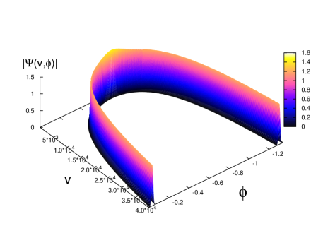
Figure 1: The evolution of a semi-classical state is shown in LQC. Unlike the Wheeler-DeWitt quantization the state does not follow the classical trajectory in to the big bang, but bounces to a contracting branch at Planck scale. The lattice chosen in this quantization is $\epsilon=2\lambda_{\beta}$, $p_{\phi}^{*}=5000$ (in Planck units) and $\Delta p_{\phi}/p_{\phi}^{*}=0.025$. As can be seen the state remains sharply peaked through out the evolution preserving semi-classicality.

Figs 1. and 2, show the result of evolution for such states. The main features are (for details see Refs. [7, 8, 11]):

1. States which are semi-classical at late times when evolved backward towards the big bang follow the classical trajectory till they reach close to the Planck scale. To be precise, the classical theory is an excellent approximation to LQC till spacetime curvature $R\sim-0.3\pi/{\ell}_{\rm Pl}^{2}$. At higher scales, departures from GR become significant. At $R=R_{\mathrm{crit}}:=-13.12/{\ell}_{\rm Pl}^{2}$ ($\rho=\rho_{\mathrm{crit}}:=\sqrt{3}/(16\pi^{2}\gamma^{3}G^{2}\hbar)=0.82\rho_{\mathrm{Planck}}$) the state bounces. The quantum bounce is non-singular and to a contracting branch with the same value of $p_{\phi}$. The big bang singularity is avoided.

2. In comparison, the states evolved using Wheeler-DeWitt quantum constraint follow the classical trajectory in to the big bang. Wheeler-DeWitt quantization does not cure the big bang singularity.

3. States remains sharply peaked through out the evolution in LQC. The relative dispersion of observables remains small before and after the bounce (though they may not be equal). Semi-classicality is preserved across the bounce.

4. Effects originating from the inverse triad terms in the gravitational and matter constraint turn out to be negligible compared to those from the field strength. In fact, even if one chooses not to regulate the inverse triad terms which diverge classically at the big bang, one will obtain a very similar evolution as in LQC for states which are semi-classical at late times i.e. for states which lead to a large classical universe. It is to be emphasized that in the flat model the inverse triad is not tied to the spacetime curvature. In fact, no meaningful physics can be associated to the scale at which inverse triad effects become dominant. A reason being that this scale is not independent under the rescaling freedom of the fiducial cell (for details see Appendix B2 of Ref. [8]). In contrast, the field strength which measures the extrinsic curvature of the spacetime leads to effects occurring at invariant scales. In the closed $k=1$ model, since the intrinsic curvature is non-zero, modifications coming from eigenvalues of the inverse triad operator do lead to meaningful physics and an interesting phenomenology, for example a non-inflationary possibility to generate scalar invariant fluctuations through thermal mechanisms in the early universe [20].

   

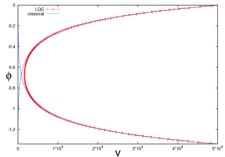
   Figure 2: Plot of the trajectories from LQC and the classical theory. Classical GR is an excellent approximation to LQC till the state reaches Planck scale. Significant departures occur beyond $\rho\sim 0.02\rho_{\mathrm{Planck}}$. The trajectory from effective Hamiltonian (not shown above) is in excellent agreement with the LQC curve.

5. Using geometric methods of quantum mechanics it is possible to write an effective Hamiltonian which describes the underlying quantum dynamics to an excellent approximation. This Hamiltonian is given by [8]

   $$\frac{3}{\gamma^{2}}\frac{\sin^{2}(\lambda_{\beta}\beta)}{\lambda_{\beta}^{2}}|p|^{3/2}=8\pi G\,H_{\mathrm{matt}}~{}.$$ (23)

   The success of the effective Hamiltonian has been extensively tested for matter with equation of state $w=1$ (massless scalar) to $w=-1$ (cosmological constant). Using Hamilton’s equations, we can derive the modified Friedman equation

   $$H^{2}=\frac{8\pi G}{3}\,\rho\left(1-\frac{\rho}{\rho_{\mathrm{crit}}}\right)$$ (24)

   and the Raychaudhuri equation

   $$\frac{\ddot{a}}{a}=-\frac{4\pi G}{3}\,\rho\,\left(1-4\frac{\rho}{\rho_{\mathrm{crit}}}\right)-4\pi G\,P\,\left(1-2\frac{\rho}{\rho_{\mathrm{crit}}}\right)~{}.$$ (25)

   These two equations result in an unmodified conservation law. For $\rho\ll\rho_{\mathrm{crit}}$, the modified Friedman equations reduce to the classical Friedman equations (6). From the loop quantum modified Friedman dynamics it is easy to see that when $\rho=\rho_{\mathrm{crit}}$, the Hubble rate becomes zero and the universe bounces. In the Planck regime the state, which we evolve backward from a large classical universe, is peaked at the effective trajectory obtained from the above equations.

The early quantization in LQC (also known as $\mu_{o}$ quantization) [5, 6] was lacking in various features as described above [9]. The difference was in the way field strength tensor is regulated. In the old quantization assignment of areas of the loop with respect to the physical geometry is not considered. Instead, the affine parameter $\lambda$ was assumed to be a constant. The resulting difference equation was of uniform step in the triad ($\mu$) and not in the volume ($\nu$). The quantization predicts a bounce but it occurs at a scale which depends on the size of fiducial cell. Thus the scale at which ‘quantum gravity’ becomes significant can be changed arbitrarily leading to unphysical effects. Such effects include a generic recollapse of a universe at late times when dominated by matter which violates strong energy condition [15]. (For an exact solution of recollapse see Ref. [22]). To understand these issues it is useful to note some features of the phase space variables.

Underlying freedoms of coordinates and cell: For the FRW metric

$${\rm d}s^{2}=-{\rm d}t^{2}+a(t)^{2}\,{\rm d}{\bf x}^{2}$$ (26)

there exists a freedom to rescale the coordinates $x\rightarrow lx$ leaving the metric invariant. This implies $a\rightarrow l^{-1}a$ and $V_{o}\rightarrow l^{3}V_{o}$. Under this freedom, the connection and triad are unaffected: $c\rightarrow c$ and $p\rightarrow p$.

However, there exists another freedom – to change only the size of the fiducial cell which amounts to changing the limits of fiducial interval of integration over coordinates: ${\cal V}\rightarrow{\cal V}^{\prime}$ such that $V_{o}^{\prime}=\alpha^{3}\,V_{o}$. Under this change,

$$c\rightarrow\alpha c~{}~{}\mathrm{and}~{}~{}p\rightarrow\alpha^{2}p.$$ (27)

Variation of phase space variables: For a general form of matter with a fixed equation of state $w$, the conservation law (obtained from Friedman and Raychaudhuri equation) leads to $\rho\propto a^{-3(1+w)}$, implying

$$c\,=\,\gamma\dot{a}\,\propto\,a^{(-3w+1)/2}~{}.$$ (28)

Thus for all matter violating strong energy condition $w<-1/3$, the connection increases as the universe expands. This is different from the behavior of spacetime curvature measured for example by the Ricci scalar which scales as $R\propto a^{-3(1+w)}$.

Thus, connection $c$ is neither invariant under the freedom of the choice of the cell nor it faithfully captures the aspects of spacetime curvature. From above properties, it is easy to see that the variable $\beta=c/|p|^{1/2}$ which is naturally selected by a consistent regularization of the field strength, is invariant under various freedoms and also scales the same way as the energy density and the curvature.

Let us now consider the effective Hamiltonian of the old quantization [9]:

$$\frac{3}{\gamma^{2}}\frac{\sin^{2}(\lambda c)}{\lambda^{2}}|p|^{1/2}=8\pi G\,H_{\mathrm{matt}}~{}.$$ (29)

It leads to the modified Friedman equation in the same form as the above except that $\rho_{\mathrm{crit}}$ is not a constant. The value of $\rho_{\mathrm{crit}}$ can be directly obtained from the effective Hamiltonian by computing the energy density at which $\sin(\lambda c)$ term saturates. Since $c$ is not invariant under the rescalings of the fiducial cell, we find that the saturation of $\sin(\lambda c)$ is not independent of $V_{o}$. This is precisely the reason for $\rho_{\mathrm{crit}}$ to depend on $V_{o}$ and the origin of various unphysical results in the old quantization. As an example, for the massless scalar case $\rho_{\mathrm{crit}}\propto 1/p_{\phi}$ which in turn scales with the change in ${\cal V}$.

Using the properties of $\beta$ as noted above, a similar argumentation for the effective Hamiltonian (23) leads to the conclusion that in the new quantization, bounce occurs at invariant curvature scale and there are no departures from general relativity for matter which satisfies null energy condition.

Remark: In literature there are proposals for quantization which rely on use of variables which are neither $\beta$ nor $c$, motivated from the ideas of lattice refinements [23]. Recently, it has been shown that all such proposals are plagued with similar problems as in the old quantization of LQC are physically not viable [15]. It turns out that for a class of quantizations, only one based on $\beta$ is invariant under freedoms of the choice of fiducial cell and thus lead to quantum bounce at a well defined curvature scale.

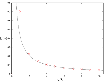
Figure 3: Eigenvalues of inverse volume are plotted in LQC (cross) and sLQC (solid). For $\nu>\lambda$ the eigenvalues quickly converge to each other. The error is 1.43% for $\nu=4\lambda$ and 0.02% for $\nu=8\lambda$ respectively.

4 Solvable LQC

The form of the quantum constraint in LQC makes extracting analytical predictions difficult and one has to rely on numerical simulations. However, by choosing lapse $N$ to be equal to the physical volume an exactly solvable model can be obtained for the matter content as a massless scalar field [17]. This model can also be obtained wth $N=1$ with mild approximations. These are based on the observation that modifications to the constraint originating from the inverse triad play negligible role on the singularity resolution and the underlying physics. There are two mild approximations involved. Setting $A(\nu)\Psi(\nu)=-12\pi{\ell}_{\rm Pl}^{2}/(\gamma\lambda_{\beta}^{2})|\nu|$ and $B(\nu)=1/(2\pi\gamma{\ell}_{\rm Pl}^{2}|\nu|)$ (the Wheeler-DeWitt value). The first approximation is innocuous since the expression is exact in LQC for $\nu=0$ and $|\nu|>\lambda_{\beta}$. The second approximation is also very mild given that departures from the actual inverse volume eigenvalues are extremely small for $\nu$ as small as $8\lambda$. The behavior of inverse volume in the Wheeler-DeWitt and LQC is shown in Fig 3. As we can see, their departures decrease rapidly when we move away from the peak of inverse volume eigenvalues in LQC at $\nu=\lambda$.

With these approximations one obtains an exactly solvable model in LQC. We emphasize that these approximations are necessary only when lapse is $N=1$. For lapse chosen equal to the volume, exactly solvable model is obtained without any approximation. The Hamiltonian constraint simplifies to

$$\partial_{\phi}^{2}\,\tilde{\Psi}(\nu,\phi)=3\pi G\,\nu\,\frac{\sin\lambda_{\beta}{\beta}}{\lambda_{\beta}}\,\nu\,\frac{\sin\lambda_{\beta}{\beta}}{\lambda_{\beta}}\,\tilde{\Psi}(\nu,\phi)=:\Theta_{(\nu)}\,\tilde{\Psi}(\nu,\phi)\,.$$ (30)

It is also possible to write the constraint in ${\beta}$ representation:

$$\partial^{2}_{\phi}\,{\chi}({\beta},\phi)=12\pi G\,\,\left(\frac{\sin\lambda_{\beta}{\beta}}{\lambda_{\beta}}\,\partial_{\beta}\right)^{2}\,\,{\chi}({\beta},\phi)$$ (31)

where $\chi({\beta},\phi)$ are Fourier transforms of $\chi(\nu,\phi)=(\lambda_{\beta}/\pi\nu)\Psi(\nu,\phi)$. The physical inner product in ${\beta}$ representation is

$$(\chi_{1},\chi_{2})_{\rm phys}=\int_{0}^{\pi/{\lambda_{\beta}}}\,{\rm d}{\beta}\,\bar{\chi}_{1}({\beta},\phi_{o})\,|\hat{\nu}|\,\chi_{2}({\beta},\phi_{o})~{}.$$ (32)

We can introduce

$$x=\frac{1}{\sqrt{12\pi G}}\,\ln\left(\tan\left(\frac{\lambda_{\beta}{\beta}}{2}\right)\right)$$ (33)

such that the quantum constraint becomes

$$\partial^{2}_{\phi}\,\,\chi(x,\phi)=\partial_{x}^{2}\,\,\chi(x,\phi)=:-\Theta\,\,\chi(x,\phi)\,.$$ (34)

General solutions can be decomposed in the left moving and right moving components: $\chi(x,\phi)=\chi_{L}(x_{+})+\chi_{R}(x_{-})$. However, the symmetry condition $\Psi(\nu,\phi)=\Psi(-\nu,\phi)$ implies $\chi(-x,\phi)=-\chi(x,\phi)$, thus

$$\chi(x,\phi)=\frac{1}{\sqrt{2}}\,(F(x_{+})-F(x_{-}))$$ (35)

where $F(x)$ are positive frequency solutions of the quantum constraint.

We can also recast the Wheeler-DeWitt theory in the ${\beta}$ representation whose constraint becomes

$$\partial^{2}_{\phi}\,\,\underline{\chi}({\beta},\phi)=-12\pi G\,\,({\beta}\,\partial_{\beta})^{2}\,\,\underline{\chi}({\beta},\phi)\,.$$ (36)

Defining

$$y:=\frac{1}{\sqrt{12\pi G}}\,\ln\frac{{\beta}}{{\beta}_{o}}$$ (37)

the constraint takes a similar form as (34):

$$\partial_{\phi}^{2}\,\,\underline{\chi}(y,\phi)=\partial_{y}^{2}\,\,\underline{\chi}(y,\phi)=:-\underline{\Theta}\,\,\underline{\chi}(y,\phi)$$ (38)

with ${\beta}_{o}$ a constant. However unlike sLQC, the left and right moving components of solutions of the Wheeler-DeWitt constraint are independent of each other. The left and right moving sectors are further left invariant by the Dirac observables: $\hat{p}_{\phi}$ and $\hat{V}|_{\phi_{o}}$. The inner product for the Wheeler-DeWitt quantization can be written as

$$(\underline{\chi}_{1},\,\underline{\chi}_{2})_{\rm phy}=\int_{-\infty}^{\infty}{\rm d}y\,\,\bar{\underline{\chi}_{1}}(y,\phi_{o})\,\,\,|\!-\!2i\partial_{y}|\,\,\,\underline{\chi}_{2}(y,\phi_{o})~{}.$$ (39)

Given the close similarity between the quantum theories of sLQC and Wheeler-DeWitt, it is necessary to bring out the key difference. It lies in the action of the volume observable. To illustrate it, let us consider the volume observables in Wheeler-DeWitt theory and without any loss of generality focus on the left moving sector (the expanding branch):

$$(\underline{\chi}_{L},\,\hat{V}|_{\phi}\,\underline{\chi}_{L})_{\mathrm{phy}}=2\pi\gamma{\ell}_{\rm Pl}^{2}\,(\underline{\chi}_{L},\,\,|\hat{\nu}|\underline{\chi}_{L})_{\mathrm{phy}}=\underline{V}\,e^{\sqrt{12\pi G}\phi},$$ (40)

here $\underline{V}$ is a constant determined completely once the initial data is specified. Thus for any given state, the volume observable diverges as $\phi\rightarrow\infty$ and vanishes when $\phi\rightarrow-\infty$. The backward evolution leads to a big bang singularity for all the states in Wheeler-DeWitt theory.

The volume observable in sLQC yields

$$(\chi,\,\,\hat{V}|_{\phi}\,\chi)_{\mathrm{phy}}=2\pi\gamma{\ell}_{\rm Pl}^{2}\,(\chi,\,\,|\hat{\nu}|\chi)_{\mathrm{phy}}=V_{+}\,e^{\sqrt{12\pi G}\phi}+V_{-}\,e^{-\sqrt{12\pi G}\phi}~{}.$$ (41)

Here $V_{+}$ and $V_{-}$ are positive definite constants determined by the initial data. Unlike the Wheeler-DeWitt theory the volume observable becomes infinite both in asymptotic future and past, attaining a minimum volume $V_{\mathrm{min}}=2\sqrt{V_{+}V_{-}}/||\chi||^{2}$ at

$$\phi_{\mathrm{bounce}}=\frac{1}{(2\sqrt{12\pi G})}\log(V_{-}/V_{+}).$$ (42)

Thus, in sLQC for any state, the backward evolution leads to a quantum bounce. The exactly solvable model enables us to extend the results obtained from numerical simulations in LQC using semi-classical states at late time to a dense subspace of the physical Hilbert space. We summarize the main results below:

1. Critical energy density as the supremum: We can construct energy density observables and consider their expectation values for general states $\chi(x,\phi)$. It turns out that the energy density has an absolute upper bound in the physical Hilbert space equal to the $\rho_{\mathrm{crit}}$ observed in the numerical simulations and the effective dynamics of LQC.

2. Issues of semi-classicality: For a very large class of states, the relative dispersion in observables is preserved across the bounce. These states include the ones with arbitrary squeezing. For more general states, the asymmetry in relative dispersion across the bounce is significantly bounded by the initial dispersion in the conjugate variables. Though the relative dispersion may be different in the expanding and the contracting branch, the resulting states are still peaked extremely well on the classical trajectories. As an example for a universe which grows to the size of a 1 MegaParsec the difference in the relative dispersion across the bounce is bounded by $10^{-56}$. If one starts with a state which is sharply peaked in the conjugate variables in a large classical universe, one gets a state which is sharply peaked on the classical trajectory after the bounce. Semi-classicality is preserved to an excellent degree across the bounce [17].

3. Comparison between sLQC and Wheeler-DeWitt: This question is tied to the possibility of turning off the quantum geometry effects by taking the limit $\Delta\rightarrow 0$. It can be shown that for a given fixed value of $\Delta>0$ and an $\varepsilon>0$, there exists a finite time interval such that sLQC and Wheeler-DeWitt approximate each other within $\varepsilon$. However, for a global time evolution the predictions of the theory will be drastically different.

4. Fundamental discreteness of sLQC: As in the case of Wheeler-DeWitt and sLQC, we can compare two sLQC theories with different $\Delta$ parameters. We then find that sLQC does not admit a limit when $\Delta\rightarrow 0$. The use of area gap to regulate field strength is a necessity in LQC which leads to its fundamental discreteness.

Summary

Loop quantum cosmology via the incorporation of non-perturbative quantum gravity effects has given useful insights on the quantum nature of the big bang. Its success lies in overcoming the limitations of the Wheeler-DeWitt quantum cosmology. From the studies of simplest models the emerging picture resolves the big bang singularity. The quantum geometric effects lead to significant departures from classical GR at Planck scale leading to a quantum bounce. The spacetime does not end at the big bang singularity, as in classical GR, but extends in to a pre-big bang branch joined with the post big-bang branch through a quantum gravitational bridge. The evolution in the Planck regime is fully deterministic. Interestingly, for states which correspond to a large classical universe at late times, it is possible to write an effective Hamiltonian and obtain modified Friedman dynamics which leads to an interesting phenomenology with implications for inflation and cyclic models [27].

Lessons from failures of old quantization in LQC and limitations of various other proposals must be incorporated to develop richer models providing a realistic description of our Universe [15]. It is pertinent to ask [28]: Whether the results of singularity resolution are artifacts of the symmetries of the cosmological spacetimes or are more general features of the quantum theory? Is there a non-singularity theorem and a non-singular Raychaudhuri equation in general? Current research in the field is aimed to investigate these issues [29].

References

References

- [1] A. Ashtekar, J. Lewandowski, Class. Quant. Grav. 21, R53 (2004) arXiv:gr-qc/0404018; C. Rovelli, “Quantum Gravity”, (Cambridge U. Press, 2004); T. Thiemann, “Modern canonical quantum general relativity,” (Cambridge U. Press, 2007).
- [2] A. Corichi, J. Phys.: Conf. Ser. 140 012006 (2008).
- [3] For recent developments in this direction, see for example, C. Rovelli, Phys. Rev. Lett. 97, 151301 (2006), arXiv:gr-qc/0508124; E. Bianchi, L. Modesto, C. Rovelli, S. Speziale, Class. Quant. Grav. 23, 6989 (2006), arXiv:gr-qc/0604044; J. Engle, R. Pereira, C, Rovelli, Phys. Rev. lett. 99, 161301 (2007), arXiv:0705.2388 [gr-qc]; E. R. Livine, S. Speziale, Phys. Rev. D 76, 084028 (2007), arXiv:0705.0674 [gr-qc]; L. Freidel, K. Krasnov, arXiv:0708.1595.
- [4] A. Ashtekar, Nuovo Cimento 112B, 1-20 (2007), arXiv:gr-qc/0702030; A. Ashtekar, arXiv:0812.0177.
- [5] A. Ashtekar, M. Bojowald and L. Lewandowski, Adv. Theor. Math. Phys. 7 233 (2003) arXiv:gr-qc/0304074.
- [6] M. Bojowald, Living Rev. Rel. 8, 11 (2005) arXiv:gr-qc/0601085.
- [7] A. Ashtekar, T. Pawlowski and P. Singh, Phys. Rev. Lett. 96, 141301 (2006), arXiv:gr-qc/0602086.
- [8] A. Ashtekar, T. Pawlowski and P. Singh, Phys. Rev. D74, 084003, arXiv:gr-qc/0607039.
- [9] A. Ashtekar, T. Pawlowski and P. Singh, Phys. Rev. D73, 124038, arXiv:gr-qc/0604013.
- [10] L. Szulc, W. Kaminski, J. Lewandowski, Class. Quant. Grav. 24, 2621 (2007) arXiv:gr-qc/0612101.
- [11] A. Ashtekar, T. Pawlowski, P. Singh, K. Vandersloot, Phys.Rev. D 75 (2007) 024035; arXiv:gr-qc/0612104.
- [12] K. Vandersloot, ‘Phys.Rev. D 75 (2007) 023523; arXiv:gr-qc/0612070.
- [13] A. Ashtekar, T. Pawlowski, P. Singh, (In preparation).
- [14] A. Ashtekar, A. Corichi, P. Singh, Phys. Rev. D 77, 024046 (2008), arXiv:0710.3565 [gr-qc].
- [15] A. Corichi and P. Singh, Phys. Rev. D 78, 024034 (2008), arXiv:0806.2783.
- [16] G. Date, arXiv:0704.0145 [gr-qc].
- [17] A. Corichi and P. Singh, Phys. Rev. Lett. 100, 161302 (2008), arXiv:0710.4543 [gr-qc].
- [18] A. Ashtekar, E. Wilson-Ewing, arXiv:0805.3511.
- [19] T. Thiemann, Class. Quant. Grav. 15, 1281 (1998), arXiv:gr-qc/9705019.
- [20] J. Magueijo, P. Singh, Phys. Rev. D 76, 023510 (2007); arXiv:astro-ph/0703566.
- [21] Y. Shtanov, V. Sahni, Phys. Lett. B 557, 1 (2003), arXiv:gr-qc/0208047.
- [22] J. Mielczarek, T. Stachowiak, M. Szydlowski, arXiv:0801.0502 [gr-qc].
- [23] M. Bojowald, Gen. Rel. Grav. 38, 1771 (2006) arXiv:gr-qc/0609034.
- [24] M. Bojowald, arXiv:0710.4919 [gr-qc].
- [25] A. Corichi, P. Singh, Phys. Rev. Lett. 101, 209002 (2008) arXiv:0811.2983.
- [26] T. Padmanabhan, J. V. Narlikar, Nature 295, 677 (1982).
- [27] See for example, M. Sami, P. Singh, S. Tsujikawa, Phys. Rev. D 74, 043514 (2006) arXiv:gr-qc/0605113; P. Singh, K. Vandersloot, G. V. Vereshchagin, Phys. Rev. D 74, 043510 (2006), arXiv:gr-qc/0606032; A. A. Sen, Phys. Rev. D 74, 043501 (2006), arXiv:gr-qc/0604050; H-H Xiong, J-Y Zhu, Phys. Rev. D 75, 084023 (2007), arXiv:gr-qc/0702003; D. Samart, B. Gumjudpai, Phys. Rev. D 76, 043514 (2007) arXiv:0704.3414 [gr-qc]; T. Naskar, J. Ward, Phys. Rev. D 76, 063514 (2007) arXiv:0704.3606 [gr-qc]; X. Zhang, Y Ling, JCAP 0708, 012 (2007), arXiv:0705.2656; H. Wei, S. N. Zhang, Phys. Rev. D 76, 063005 (2007), arXiv:0705.4002; G. De Risi, R. Maartens, P. Singh, Phys. Rev. D 76, 103531 (2007), arXiv:0706.3586; E. J. Copeland, D. J. Mulryne, N. J. Nunes, Phys. Rev. D 77, 023510 (2008), arXiv:0708.1261 [gr-qc].
- [28] N. Dadhich, arXiv:gr-qc/0702095.
- [29] For ongoing works on ansitropies and Gowdy spacetimes see, D-W. Chiou, Phys. Rev. D 75, 024029 (2007), arXiv:gr-qc/0609029; D-W. Chiou, K. Vandersloot Phys. Rev. D 76, 084015 (2007), arXiv:gr-qc/0707.2548 [gr-qc]; K. Banerjee, G. Date, arXiv;0712.0687 [gr-qc].