ITEP-TH-01/09
LPTENS-09/01
UUITP-01/09

1 Introduction

The ABJM model [1] has opened up a new avenue in which to explore integrability in the planar limit of gauge theories in three dimensions. This model is comprised of two $U(N)$ gauge groups having a Chern-Simons action with levels $k$ and $-k$ respectively. The model also contains scalars and fermions that live in the bifundamental representations of $U(N)\times U(N)$. If the six scalar and two scalar-two fermion couplings are properly tuned [1, 2, 3], then the theory has an ${\cal N}=6$ supersymmetry. This then leads to an $SO(6)\simeq SU(4)$ $R$-symmetry, with the $(N,\bar{N})$ scalars transforming in the 4 while the $(N,\bar{N})$ fermions transform in the $\bf\bar{4}$, with an appropriate $R$-symmetry assignment for the conjugates. This theory also has a CP invariance. The Chern-Simons action changes sign under parity, but can also be accompanied by an exchange of the gauge groups to restore the sign.

Chern-Simons-matter theories admit a planar limit when the rank of the gauge group and the Chern-Simons level simultaneously approach infinity such that their ratio $\lambda=N/k$ remains finite. The operator mixing problem can then be reformulated in terms of a quantum spin chain whose interaction range grows with the order of perturbation theory. Interesting effects in Chern-Simons-matter theories start at two loops [4], and with one loop terms absent the leading order spin-chain Hamiltonian involves three-site next-to-nearest-neighbor interactions [5]. Such spin chains are usually not integrable, which is indeed the case for the $\mathcal{N}=1$ superconformal Chern-Simons [5]. However, in [6] it was shown that the scalar sector of the $\mathcal{N}=6$ ABJM theory is integrable at two loops (see also [7]). The corresponding spin chain is made up of alternating sites of 4 and $\bf\bar{4}$ spins, and the Hamiltonian contains terms up to next to nearest neighbor interactions. The CP invariance of the gauge theory results in a parity invariance for the spin chain. The Bethe ansatz for this spin-chain was given and was shown to lead to correct results for the anomalous dimensions of scalar operators. A conjectured Bethe ansatz was also given for the full superconformal group $OSp(6|4)$. This Bethe ansatz is consistent with results from the $SU(2|2)$ sector which was also shown to be integrable [8]. Furthermore, these Bethe ansätze were extended to an all-loop Bethe ansatz [9, 10]. Other interesting results related to the integrability of the ABJM model have been found in [11, 12, 13, 14, 15, 16, 17, 18, 19, 20, 21, 22, 23, 24, 25, 26, 27, 28, 29, 30, 31, 32, 33].

In another development, Aharony, Bergman and Jafferis (ABJ) extended the ABJM analysis to include among other things an asymmetric theory with gauge group $U(N)\times U(\hat{N})$ [34]. Such a theory is no longer CP invariant if $N\neq\hat{N}$, but has all the same continuous symmetries as the $N=\hat{N}$ ABJM model [3]. One would then expect that the parity invariance of the spin chain is broken. This does not necessarily mean that the integrability is lost, there are integrable spin chains with broken parity [35].

Nevertheless, one can give a general argument that the ABJ model should not be integrable. The argument is based on the dual description in terms of type IIA string theory on an $AdS_{4}\times CP^{3}$ background [1, 34]. The integrability of the spin chain is reflected in the classical integrability of the string sigma-model [11, 12, 13], which may, or may not be preserved at the quantum level. The different ranks in the ABJ model means that there are two ’t Hooft couplings, $\lambda=N/k$ and $\hat{\lambda}=\hat{N}/k$, and their difference leads to a theta-angle on the string world-sheet: $\vartheta_{\rm w.s.}\sim\lambda-\hat{\lambda}$ [34], which is responsible for world-sheet parity violation, analogous to potential parity violation in the spin chain. However, it is commonly believed that the theta-angle and parity violation destroy integrability. We can draw an analogy with the $O(3)$ non-linear sigma-model which is integrable at $\vartheta=0$ and $\vartheta=\pi$, but presumably is not integrable at generic $\vartheta$ [37]. The analogy with the $O(3)$ model is arguably far-fetched, the supercoset sigma-model on $AdS_{4}\times CP^{3}$ is quite different. So, our argument is only qualitative, and it would be very interesting to check if the ABJ model is integrable or not for generic $\lambda$ and $\hat{\lambda}$. At strong coupling, the dependence on the difference $\lambda-\hat{\lambda}$ is very weak, since the world-sheet instanton effects which are sensitive to the theta-angle are exponentially suppressed. But at weak coupling, one has no reason to think that that the anomalous dimensions will depend on the geometric mean of the ’t Hooft couplings, $\lambda\hat{\lambda}$, and not on their difference, $\lambda-\hat{\lambda}$ which is the measure of parity violation.

Nonetheless, somewhat surprisingly, it was shown that the parity invariance and with it the integrability in the scalar sector is still preserved at the two loop level for generic $\lambda$ and $\hat{\lambda}$ [35]. In principle, two loop corrections could come with factors of $\lambda^{2}$, $\hat{\lambda}^{2}$ or $\lambda\hat{\lambda}$. But one can quickly see that in the scalar sector, only diagrams with factors of $\lambda\hat{\lambda}$ appear. Hence the parity is unbroken and the integrability is preserved, with all factors of $\lambda^{2}$ in the ABJM spin chain replaced by $\lambda\hat{\lambda}$ in the more general ABJ case.

Going outside the scalar sector, one does find diagrams that are proportional to $\lambda^{2}$ and $\hat{\lambda}^{2}$, so it is possible that only the scalar sector is integrable. Moreover, the integrability of the full ABJM model is only a conjecture and has to be verified, especially in view of the discrepancies that have arisen between string theory results [38, 39, 40, 41] and those derived from the algebraic curve [13, 9, 42].

In this paper we will explore these issues by first considering gauge invariant operators with one fermion present. Here we will find that there are loop diagrams that lead to possible $\lambda^{2}$ and $\hat{\lambda}^{2}$ terms. However, these diagrams cancel off with other diagrams, resulting in a dilatation operator with $\lambda\hat{\lambda}$ terms only. We compute the dilation operator for all operators of this type and explicitly show that it is consistent with the proposed Bethe ansatz in [6] for operators of length 4.

We then go on to construct the general Hamiltonian for the full $OSp(6|4)$. We do this by first constructing it for an $SL(2|1)\simeq OSp(2|2)$ sector, a noncompact closed sector containing fermions. In fact the $R$-matrices for noncompact $SL(2|1)$ have previously appeared in the literature [43, 44]. The Hamiltonian is written in terms of projectors onto irreducible representations of $SL(2|1)$. The results for $SL(2|1)$ can then be uniquely lifted to the full $OSp(6|4)$ in a way analogous to how the $SU(1,1)$ sector of ${\cal N}=4$ Super Yang-Mills is lifted to the full $PSU(2,2|4)$ superconformal group [48, 49]. The difference here is that for this spin chain the $R$-matrices are built out of two complex representations, while in $SU(1,1)$ the $R$-matrix is built using a single real representation.

In section 2 we review the Lagrangian of ${\cal N}=6$ superconformal Chern-Simons as well as the conjectured two-loop Bethe equations for all single trace operators. In section 3 we derive the Hamiltonian for the spin chain with one fermion present by computing the appropriate Feynman diagrams. In section 4 we compute the anomalous dimensions for all length 4 operators with one fermion and show that the conjectured Bethe equations give the correct result. In section 5 we construct the Hamiltonian for the full $OSp(6|4)$. We do this by taking the $R$-matrix for the $SL(2|1)$ subgroup and extending it to $OSp(6|4)$. We then show that the resulting Hamiltonian is consistent with the Hamiltonian for scalar operators and the Hamiltonian derived in section 3 for operators with one fermion. In section 6 we give a short discussion.

Note added: As this paper was being prepared we received [50] which overlaps with our results in section 5.

2 The ${\cal N}=6$ theory and its Bethe equations

In this section we give a short review of the ABJM ${\cal N}=6$ superconformal Chern-Simons theory and the conjectured two-loop Bethe equations that arise from it.

The lagrangian of the $\mathcal{N}=6$ Chern-Simons theory is [1, 2, 3]

$$\mathcal{L} = \frac{k}{4\pi}\,{\rm tr}\,\left[\varepsilon^{\mu\nu\lambda}\left(A_{\mu}\partial_{\nu}A_{\lambda}+\frac{2}{3}\,A_{\mu}A_{\nu}A_{\lambda}-\hat{A}_{\mu}\partial_{\nu}\hat{A}_{\lambda}-\frac{2}{3}\,\hat{A}_{\mu}\hat{A}_{\nu}\hat{A}_{\lambda}\right)\right.$$ (2.1)

$$\left.+D_{\mu}Y^{\dagger}_{A}D^{\mu}Y^{A}+i\bar{\psi}^{A}D\!\!\!\!/\,\psi_{A}+\frac{1}{12}\,Y^{A}Y^{\dagger}_{A}Y^{B}Y^{\dagger}_{B}Y^{C}Y^{\dagger}_{C}+\frac{1}{12}\,Y^{A}Y^{\dagger}_{B}Y^{B}Y^{\dagger}_{C}Y^{C}Y^{\dagger}_{A}\right.$$

$$\left.-\frac{1}{2}\,Y^{A}Y^{\dagger}_{A}Y^{B}Y^{\dagger}_{C}Y^{C}Y^{\dagger}_{B}+\frac{1}{3}\,Y^{A}Y^{\dagger}_{B}Y^{C}Y^{\dagger}_{A}Y^{B}Y^{\dagger}_{C}\right.$$

$$\left.-\frac{1}{2}\,Y^{\dagger}_{A}Y^{A}\bar{\psi}^{B}\psi_{B}+Y^{\dagger}_{A}Y^{B}\bar{\psi}^{A}\psi_{B}+\frac{1}{2}\,\bar{\psi}^{A}Y^{B}Y^{\dagger}_{B}\psi_{A}-\bar{\psi}^{A}Y^{B}Y^{\dagger}_{A}\psi_{B}\right.$$

$$\left.+\frac{1}{2}\,\varepsilon^{ABCD}Y^{\dagger}_{A}\bar{\psi}_{cB}Y^{\dagger}_{C}\psi_{D}-\frac{1}{2}\,\varepsilon_{ABCD}Y^{A}\bar{\psi}^{B}Y^{C}C\psi_{c}^{D}\right],$$

where $D_{\mu}X=\partial X+A_{\mu}X-X\hat{A}_{\mu}$, $D_{\mu}X^{\dagger}=\partial_{\mu}X^{\dagger}+\hat{A}_{\mu}X^{\dagger}-X^{\dagger}A_{\mu}$. We use the $+--$ conventions for the metric. Raised capital latin indices (A,B,C,D) are $SU(4)$ $R$-symmetry indices for the fundamental representation, while lowered indices of this type are for the anti-fundamental representation. In the last two terms, $\psi_{c}^{A}$ is the charge conjugated fermion field, $\psi_{c}^{A}=C\gamma_{0}\,\psi_{A}^{*}$, where $C$ is the charge conjugation matrix: $\gamma_{\mu}C+C\gamma_{\mu}^{T}=0$, $C^{2}=1$, $C^{\dagger}=C$, and $C^{T}=-C$. The Dirac matrices satisfy

$$\gamma^{\mu}\gamma^{\nu}=\eta^{\mu\nu}+i\varepsilon^{\mu\nu\lambda}\gamma_{\lambda},$$ (2.2)

with $\varepsilon^{012}=1=\varepsilon_{012}$. The form of the Lagrangian is the same for the ABJ model where the number of colors for the two gauge groups, $N$ and $\hat{N}$, are no longer equal.

The ABJM model is conformally invariant. Its Hilbert space consists of all possible local operators, which at tree level are highly degenerate. The degeneracy is lifted by quantum corrections and leads to a fairly complicated mixing pattern. The mixing matrix can be calculated in perturbation theory, and in the large-$N$ limit can be identified with the Hamiltonian of a quantum spin chain. Computation of the full mixing matrix is a formidable task even at the leading two-loop order, and we will first consider closed sectors for which the Hamiltonian can be evaluated directly from Feynman diagrams with relative ease. One such sector is comprised of the bosonic operators:

$$\mathop{\mathrm{tr}}Y^{A_{1}}Y^{\dagger}_{B_{1}}Y^{A_{2}}Y^{\dagger}_{B_{2}}\dots Y^{A_{L}}Y^{\dagger}_{B_{L}},$$ (2.3)

which form a basis of states in the closed alternating spin chain with $SU(4)$ symmetry. The spin chain Hamiltonian is [6, 35]

$$\mathnormal{\Gamma}_{{\rm bos}}=\frac{\lambda\hat{\lambda}}{2}\sum_{l=1}^{2L}\left(2-2P_{l,l+2}+P_{l,l+2}K_{l,l+1}+K_{l,l+1}P_{l,l+2}\right),$$ (2.4)

where $K_{ll^{\prime}}$ and $P_{ll^{\prime}}$ are the trace and permutation operators acting on the $l$th and $l^{\prime}$th sites of the lattice: $P^{AA^{\prime}}{}_{BB^{\prime}}=\delta^{A}{}_{B^{\prime}}\,\delta^{A^{\prime}}{}_{B}$, $K^{A}_{A^{\prime}}\,{}^{B^{\prime}}_{B}=\delta^{A}{}_{B}\,\,\delta_{A^{\prime}}{}^{B^{\prime}}$.

In [6] a set of Bethe equations was given that are consistent with the Hamiltonian in (2.4). Based on the $OSp(6|4)$ superconformal algebra, an extended set of Bethe equations were conjectured valid for all operators. These equations are

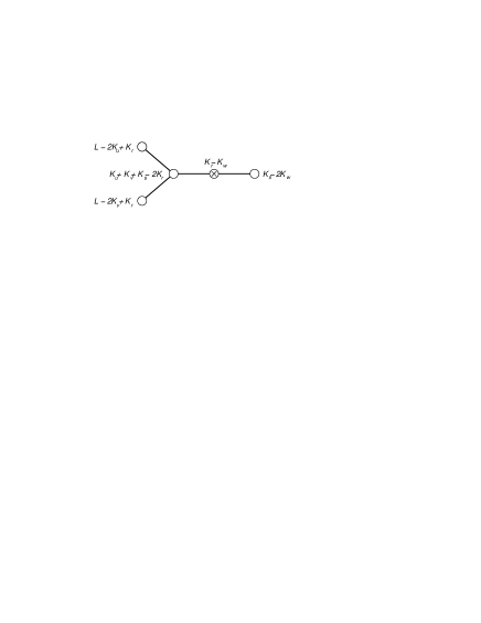
Figure 1: The Dynkin diagram of $OSp(6|4)$. Shown are the Dynkin labels of the state with $\{K_{u},K_{v},K_{r},K_{s},K_{w}\}$ Bethe roots.

$$\left(\frac{u_{j}+i/2}{u_{j}-i/2}\right)^{L} = \prod_{k=1,k\neq j}^{K_{u}}\frac{u_{j}-u_{k}+i}{u_{j}-u_{k}-i}\prod_{k=1}^{K_{r}}\frac{u_{j}-r_{k}-i/2}{u_{j}-r_{k}+i/2}$$

$$\left(\frac{v_{j}+i/2}{v_{j}-i/2}\right)^{L} = \prod_{k=1,k\neq j}^{K_{v}}\frac{v_{j}-v_{k}+i}{v_{j}-v_{k}-i}\prod_{k=1}^{K_{r}}\frac{v_{j}-r_{k}-i/2}{v_{j}-r_{k}+i/2}$$

$$1 = \prod_{k=1,k\neq j}^{K_{r}}\frac{r_{j}-r_{k}+i}{r_{j}-r_{k}-i}\prod_{k=1}^{K_{u}}\frac{r_{j}-u_{k}-i/2}{r_{j}-u_{k}+i/2}\prod_{k=1}^{K_{v}}\frac{r_{j}-v_{k}-i/2}{r_{j}-v_{k}+i/2}\prod_{k=1}^{K_{s}}\frac{r_{j}-s_{k}-i/2}{r_{j}-s_{k}+i/2}$$

$$1 = \prod_{k=1}^{K_{r}}\frac{s_{j}-r_{k}-i/2}{s_{j}-r_{k}+i/2}\prod_{k=1}^{K_{w}}\frac{s_{j}-w_{k}+i/2}{s_{j}-w_{k}-i/2}$$

$$1 = \prod_{k=1,k\neq j}^{K_{w}}\frac{w_{j}-w_{k}-i}{w_{j}-w_{k}+i}\prod_{k=1}^{K_{s}}\frac{w_{j}-s_{k}+i/2}{w_{j}-s_{k}-i/2}\,.$$ (2.5)

The first three lines in (2) are the Bethe equations of scalar operators when $K_{s}=0$. The Bethe equations correspond to the Dynkin diagram in fig. 1. The excitation numbers $K_{a}$ must satisfy a set of inequalities (which are basically the highest-weight conditions for the Bethe wave functions):

$$L-2K_{u}+K_{r} \geqslant 0$$

$$L-2K_{v}+K_{r} \geqslant 0$$

$$K_{u}+K_{v}-2K_{r}+1 \geqslant 0$$

$$K_{r} > K_{s}$$

$$K_{s}-2K_{w} \geqslant 0.$$ (2.6)

The solutions that correspond to gauge-theory operators in addition satisfy the level-matching (zero-momentum) condition,

$$\prod_{j=1}^{K_{u}}\frac{u_{j}+i/2}{u_{j}-i/2}\prod_{j=1}^{K_{v}}\frac{v_{j}+i/2}{v_{j}-i/2}=1.$$ (2.7)

The anomalous dimensions for the operators are eigenvalues of the Hamiltonian for the spin chain, and are given by

$$\gamma=\lambda\hat{\lambda}\left(\sum_{j=1}^{K_{u}}\frac{1}{u_{j}^{2}+\frac{1}{4}}+\sum_{j=1}^{K_{v}}\frac{1}{v_{j}^{2}+\frac{1}{4}}\right).$$ (2.8)

Notice that only the $u_{j}$ and $v_{j}$ Bethe roots contribute to (2.7) and (2.8). Only these roots carry momentum and energy.

3 Fermionic part of the dilatation operator

In this section we study operators with a single fermion insertion,

$$\mathop{\mathrm{tr}}\psi_{B}Y^{\dagger}_{B_{1}}Y^{A_{2}}Y^{\dagger}_{B_{2}}\dots Y^{A_{L}}Y^{\dagger}_{B_{L}}\qquad{\rm and}\qquad\mathop{\mathrm{tr}}Y^{A_{1}}\psi_{c}^{A}Y^{A_{2}}Y^{\dagger}_{B_{2}}\dots Y^{A_{L}}Y^{\dagger}_{B_{L}}.$$ (3.1)

They also form a closed sector at two loops because of fermion number conservation. We will compute the two-loop mixing matrix for these operators. In the bulk of the operator (far from the fermion insertion), the mixing matrix is the same as in (2.4). Here we concentrate on the mixing that involves the fermion insertion.

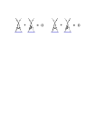
Figure 2: The CP-breaking contributions to the dilatation operator mutually cancel.

Potentially, mixing of the fermions could depend on $\lambda^{2}$ and $\hat{\lambda}^{2}$ separately and thus could break CP invariance. The $\lambda$–$\hat{\lambda}$ power counting can be easily pictured by coloring the double-line ’t Hooft diagrams. There are two gauge groups, and one can draw the $U(N)$ and $U(\hat{N})$ index lines in two different colors, say blue and red. A planar diagram will then be a collection of facets (index loops) painted in the two colors. Since the matter fields are bifundamentals and the gauge fields are adjoints, the color changes across a scalar or fermion propagator, but stays the same across a gauge or ghost propagator. A diagram with $F_{r}$ red facets and $F_{b}$ blue facets is accompanied by a factor $N^{F_{r}}\hat{N}^{F_{b}}\propto\lambda^{F_{r}}\hat{\lambda}^{F_{b}}$. It is the diagrams with $F_{r}\neq F_{b}$ that potentially violate CP. At the two-loop order there are four such diagrams, all of which involve internal gauge-boson lines. To our surprise these diagrams mutually cancel (fig. 2). The fermion part of the dilatation operator thus is also proportional to $\lambda\hat{\lambda}$:

$$\mathnormal{\Gamma}_{\rm ferm}=\frac{\lambda\hat{\lambda}}{6}({\rm const}+H),$$ (3.2)

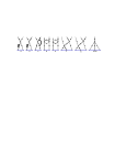
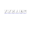
Figure 3: The diagrams that contribute to the mixing of operators with single fermion insertion.

The diagrams that contribute to the fermion mixing and that do not identically vanish are listed in fig 3. There is also a number of diagrams that do not mix different operators and only contribute to the constant term in (3.2). We have not shown these diagrams and have not computed them. The constant will be later fixed by requiring that the dilatation operator preserves supersymmetry. Each diagram in fig. 3 should be supplemented with its parity conjugate (denoted by a *), The only exception is he diagram $h$ which is its own parity-conjugate. The last two diagrams, $m$ and $n$, do not directly involve fermion interaction vertices, and one may be tempted to attribute them to the bosonic part of the mixing matrix (2.4). Indeed, these diagrams combine with the six-boson vertex to cancel off the nearest-neighbor exchanges in the bosonic part of the mixing matrix [6]. In the presence of the fermion insertion, this cancelation is incomplete. In the middle of the scalar operator, $m$ and $n$ participate in the cancelation of the six-vertex graph on the left and on the right, but now there is a fermion on the left, and half of the $m+n$ has nothing to cancel. The easiest way to take into account these diagrams is to add the nearest-neighbor term from the six-vertex graph (which can be found in eq. (2.6) of [6]) to the fermion mixing matrix with coefficient $(-1/2)$. The diagrams $h+h^{*}$ and $l$ represent mixing with a derivative of $\psi_{c}$ and $\psi$. However, because of the Lorentz invariance the derivative must be accompanied by the Dirac matrix and combined into $D\!\!\!\!/\ \psi$ or $D\!\!\!\!/\ \psi_{c}$, which can be eliminated by use of the equations of motion.

Computing the diagrams in fig. 3 is in principle straightforward. Collecting all pieces together, we get:

$$H\circ Y^{\dagger}_{A}\psi_{B}Y^{\dagger}_{C} = -2Y^{\dagger}_{A}\psi_{C}Y^{\dagger}_{B}-2Y^{\dagger}_{B}\psi_{A}Y^{\dagger}_{C}-Y^{\dagger}_{B}\psi_{C}Y^{\dagger}_{A}-Y^{\dagger}_{C}\psi_{A}Y^{\dagger}_{B}-2Y^{\dagger}_{C}\psi_{B}Y^{\dagger}_{A}$$ (3.3)

$$-6\varepsilon_{BCDE}Y^{\dagger}_{A}Y^{D}\psi_{c}^{E}-6\varepsilon_{ABDE}\psi_{c}^{D}Y^{E}Y^{\dagger}_{C}-\varepsilon_{ABCD}\psi_{c}^{D}Y^{E}Y^{\dagger}_{E}$$

$$+3\varepsilon_{ACDE}Y^{\dagger}_{B}Y^{D}\psi_{c}^{E}+3\varepsilon_{ACDE}\psi_{c}^{D}Y^{E}Y^{\dagger}_{B}+\varepsilon_{ABCD}Y^{\dagger}_{E}Y^{E}\psi_{c}^{D}$$

$$-2\varepsilon_{ABCD}Y^{\dagger}_{E}Y^{D}\psi_{c}^{E}+2\varepsilon_{ABCD}\psi_{c}^{E}Y^{D}Y^{\dagger}_{E},$$

$$H\circ\psi_{A}Y^{\dagger}_{B}Y^{C} = -3Y^{C}Y^{\dagger}_{B}\psi_{A}-3Y^{C}Y^{\dagger}_{A}\psi_{B}$$

$$+\delta_{B}^{C}Y^{D}Y^{\dagger}_{A}\psi_{D}+\delta_{B}^{C}Y^{D}Y^{\dagger}_{D}\psi_{A}+\delta_{A}^{C}Y^{D}Y^{\dagger}_{D}\psi_{B}+\delta_{A}^{C}Y^{D}Y^{\dagger}_{B}\psi_{D}$$

$$+2\delta_{B}^{C}\psi_{A}Y^{\dagger}_{D}Y^{D}-\delta_{B}^{C}\psi_{D}Y^{\dagger}_{A}Y^{D}-\delta_{A}^{C}\psi_{B}Y^{\dagger}_{D}Y^{D}+2\delta_{A}^{C}\psi_{D}Y^{\dagger}_{B}Y^{D}$$

$$+3\varepsilon_{ABDE}Y^{D}\psi_{c}^{C}Y^{E}+\delta_{B}^{C}\varepsilon_{ADEF}Y^{D}\psi_{c}^{E}Y^{F}-2\delta_{A}^{C}\varepsilon_{BDEF}Y^{D}\psi_{c}^{E}Y^{F},$$

$$H\circ Y^{A}Y^{\dagger}_{B}\psi_{C} = -3\psi_{C}Y^{\dagger}_{B}Y^{A}-3\psi_{B}Y^{\dagger}_{C}Y^{A}$$

$$+\delta_{B}^{A}\psi_{D}Y^{\dagger}_{C}Y^{D}+\delta_{B}^{A}\psi_{C}Y^{\dagger}_{D}Y^{D}+\delta_{C}^{A}\psi_{B}Y^{\dagger}_{D}Y^{D}+\delta_{C}^{A}\psi_{D}Y^{\dagger}_{B}Y^{D}$$

$$+2\delta_{B}^{A}Y^{D}Y^{\dagger}_{D}\psi_{C}-\delta_{B}^{A}Y^{D}Y^{\dagger}_{C}\psi_{D}-\delta_{C}^{A}Y^{D}Y^{\dagger}_{D}\psi_{B}+2\delta_{C}^{A}Y^{D}Y^{\dagger}_{B}\psi_{D}$$

$$+3\varepsilon_{BCDE}Y^{D}\psi_{c}^{A}Y^{E}-\delta_{B}^{A}\varepsilon_{CDEF}Y^{D}\psi_{c}^{E}Y^{F}+2\delta_{C}^{A}\varepsilon_{BDEF}Y^{D}\psi_{c}^{E}Y^{F}.$$

There are two terms in the Lagrangian (2.1) contributing to the $Y^{\dagger}Y\bar{\psi}\psi$-vertex and two terms contributing to the $\bar{\psi}YY^{\dagger}\psi$-vertex. The terms $\,{\rm tr}\,Y^{\dagger}_{A}Y^{B}\bar{\psi}^{A}\psi_{B}$ and $\,{\rm tr}\,\bar{\psi}^{A}Y^{B}Y_{A}^{\dagger}\psi_{B}$ mix the flavor indices while the other two do not. It means the diagrams with two fermion-boson vertices correspond to up to four different terms in the Hamiltonian.

To get the action of the dilatation operator on the states with a $\psi_{c}$ insertion one has to compute the same set of diagrams with the arrows on all the lines inverted. However, pulling the charge conjugation matrix through the fermion line reverses all the momenta due to the identity $-C/\!\!\!{p}^{T}=/\!\!\!{p}C$, so the result will be exactly the same. Consequently, the dilatation operator is given by interchanging the upper and lower indices in (3.3)–(3), and so making the replacement $Y^{A}\leftrightarrow Y^{\dagger}_{A}$, $\psi_{A}\leftrightarrow\psi_{c}^{A}$, $\varepsilon_{ABCD}\leftrightarrow\varepsilon^{ABCD}$, $\delta_{A}^{B}\leftrightarrow\delta_{B}^{A}$.

The constant in (3.2) can be fixed by requiring that the ground state energy is zero. The computation at length-$4$ (sec. 4) gives:

$$\mathnormal{\Gamma}_{\rm ferm}=\frac{\lambda\hat{\lambda}}{6}\left(20+H\right).$$ (3.6)

The full one-loop dilatation operator is then the sum of the mixing matrices acting on scalars, eq. (2.4), and the fermion mixing matrix (3.6),

$$\mathnormal{\Gamma}=\mathnormal{\Gamma}_{\rm bos}+\mathnormal{\Gamma}_{\rm ferm}.$$ (3.7)

4 Length-$4$ operators

In this section we will explicitly diagonalize the mixing matrix from the previous section for operators of length four. We will also solve the Bethe equations (2) for $L=2$ and compare the resulting spectra of anomalous dimensions. There are in total $2\times 4^{4}=512$ operators, but many of them are super-descendants of the bosonic length-$4$ operators $\,{\rm tr}\,(YY^{\dagger})^{2}$. The solutions of the Bethe equations describe primary operators, so first we will discuss constraints imposed on the spectrum by supersymmetry.

Under the $SU(4)$ R-symmetry, the length-$4$ states $\,{\rm tr}\,\psi Y^{\dagger}YY^{\dagger}$ and $\,{\rm tr}\,Y\psi_{c}YY^{\dagger}$ transform as

$$\bar{\mathbf{4}}\otimes\mathbf{4}\otimes\mathbf{4}\otimes\mathbf{4} = \mathbf{6}^{3}\oplus\mathbf{10}^{3}\oplus\bar{\mathbf{10}}\oplus\mathbf{64}^{2}\oplus\mathbf{70}$$ (4.1)

$$\mathbf{4}\otimes\bar{\mathbf{4}}\otimes\bar{\mathbf{4}}\otimes\bar{\mathbf{4}} = \mathbf{6}^{3}\oplus\mathbf{10}\oplus\bar{\mathbf{10}}^{3}\oplus\mathbf{64}^{2}\oplus\bar{\mathbf{70}}.$$ (4.2)

The scalar operators $\,{\rm tr}\,(YY^{\dagger})^{2}$ are in

$$\bar{\mathbf{4}}\otimes{\mathbf{4}}\otimes\bar{\mathbf{4}}\otimes{\mathbf{4}}=\mathbf{1}^{2}\oplus\mathbf{15}^{2}\oplus\mathbf{20}\oplus\mathbf{84}.$$ (4.3)

Their anomalous dimensions, in the units of $\lambda\hat{\lambda}$, are $2,10,6,6,8,0$, respectively [6].

The supercharges act on the scalars as

$$Q_{AB}Y^{C}=\delta^{C}_{A}\psi_{B}-\delta_{B}^{C}\psi_{A}$$ (4.4)

$$Q_{AB}Y^{\dagger}_{C}=\varepsilon_{ABCD}{\psi}_{c}^{D}.$$ (4.5)

Consequently,

$$Q\,{\rm tr}\,YY^{\dagger}YY^{\dagger}\sim\psi Y^{\dagger}YY^{\dagger}+Y{\psi}_{c}YY^{\dagger}.$$

Since the supercharges are in the $\mathbf{6}$ of $SU(4)$, the superpartners of the scalar operators belong to

$$\mathbf{6}\otimes\left(\mathbf{1}^{2}\oplus\mathbf{15}^{2}\oplus\mathbf{20}\oplus\mathbf{84}\right)=\mathbf{6}^{5}\oplus\mathbf{10}^{2}\oplus\bar{\mathbf{10}}^{2}\oplus\mathbf{64}^{4}\oplus\mathbf{70}\oplus\bar{\mathbf{70}}{\color[rgb]{.5,.5,.5}\oplus\mathbf{50}\oplus\mathbf{300}}.$$ (4.6)

One has to remember, however, that not all representations in the product are associated with operators. The last two representations shown in gray are projected out. This can be understood from the supersymmetry transformations (4.4), (4.5). The left-hand side of (4.4) is in $\mathbf{6}\otimes\mathbf{4}=\bar{\mathbf{4}}{\color[rgb]{.5,.5,.5}\oplus\mathbf{20}}$, but only the $\bar{\mathbf{4}}$ appears on the right-hand side. Likewise, in (4.5), which is $\mathbf{6}\otimes\bar{\mathbf{4}}=\mathbf{4}{\color[rgb]{.5,.5,.5}\oplus\bar{\mathbf{20}}}$, the $\bar{\mathbf{20}}$ is projected out.

The supersymmetry fixes part of the spectrum in (4.1), (4.2):

$$\mathbf{64}\oplus\mathbf{70}\oplus\bar{\mathbf{70}}: 0$$

$$\mathbf{6}: 2\lambda\hat{\lambda}$$

$$\mathbf{6}^{2}\oplus\mathbf{10}^{2}\oplus\bar{\mathbf{10}}^{2}\oplus\mathbf{64}^{2}: 6\lambda\hat{\lambda}$$

$$\mathbf{6}\oplus\mathbf{64}: 8\lambda\hat{\lambda}$$

$$\mathbf{6}: 10\lambda\hat{\lambda},$$ (4.7)

Hence, we are left with five multiplets whose highest-weight states are fermionic length-$4$ operators:

$$\mathbf{6}\oplus\mathbf{10}^{2}\oplus\bar{\mathbf{10}}^{2}.$$ (4.8)

We will compute their anomalous dimensions first by diagonalizing the Hamiltonian (3.3)–(3), (2.4), and then by solving the Bethe equations. We should note that the solutions of the Bethe equations for the fermion states are sensitive to the whole structure of the Dynkin diagram.

4.1 Spectrum from the mixing matrix

Let us diagonalize the Hamiltonian in (3.6). The simplest case is the $\bar{\mathbf{70}}$ operator:

$$O_{\bar{\mathbf{70}}}=\,{\rm tr}\,Y^{\dagger}_{(A}\psi_{B}Y^{\dagger}_{C)}Y^{D}-{\rm traces}.$$ (4.9)

The symmetrization acts on all three lower indices. The bosonic part of the dilatation operator annihilates $O_{\bar{\mathbf{70}}}$, because of the symmetry in $A$, $B$ and $C$. This operator does not mix with the $\psi_{c}$ states either, since such mixing inevitably involves contraction with the $\varepsilon_{ABFE}$ tensor. The rest of the Hamiltonian in (3.3)–(3) acts as

$$H\circ O_{\bar{\mathbf{70}}}=-20\,O_{\bar{\mathbf{70}}}\,.$$ (4.10)

The $\bar{\mathbf{70}}$ is a part of the BPS supermultiplet and thus should have zero anomalous dimension. This fixes the constant term in (3.6).

The next set of operators are the four states in the $\bar{\mathbf{10}}$:

$$\mathcal{O}^{\bar{\mathbf{10}}}_{1\,AB}=\,{\rm tr}\,Y^{\dagger}_{C}\psi_{(A}Y^{\dagger}_{B)}Y^{C},\qquad\mathcal{O}^{\bar{\mathbf{10}}}_{2\,AB}=\,{\rm tr}\,Y^{\dagger}_{(A}\psi_{B)}Y^{\dagger}_{C}Y^{C},$$

$$\mathcal{O}^{\bar{\mathbf{10}}}_{3\,AB}=\,{\rm tr}\,Y^{\dagger}_{(A}\psi_{C}Y^{\dagger}_{B)}Y^{C},\qquad\mathcal{O}^{\bar{\mathbf{10}}}_{4\,AB}=\,{\rm tr}\,Y^{C}{\psi}_{c}^{D}Y^{E}Y^{\dagger}_{(A}\varepsilon_{B)CDE}.$$ (4.11)

Here we also know part of the spectrum from supersymmetry, eq. (4), but in addition to the two descendants there are two highest-weight states. It turns out that the dilatation operator is fully degenerate in this sector:

$$\left.\mathnormal{\Gamma}\right|_{\mathbf{10}}=\lambda\hat{\lambda}\begin{pmatrix}6&0&0&0\\ 0&6&0&0\\ 0&0&6&0\\ 0&0&0&6\\ \end{pmatrix}$$ (4.12)

This agrees with (4), and predicts that four of the anomalous dimensions in (4.8) are equal to $6\lambda\hat{\lambda}$ (the anomalous dimensions in $\mathbf{10}$ are obviously the same as in $\bar{\mathbf{10}}$).

The basis of operators in the $\mathbf{6}$ is spanned by

$$\mathcal{O}^{\mathbf{6}}_{1\,AB}=2\,{\rm tr}\,Y^{\dagger}_{C}\psi_{[A}Y^{\dagger}_{B]}Y^{C},\qquad\mathcal{O}^{{\mathbf{6}}}_{2\,AB}=2\,{\rm tr}\,Y^{\dagger}_{[A}\psi_{B]}Y^{\dagger}_{C}Y^{C},$$

$$\mathcal{O}^{{\mathbf{6}}}_{3\,AB}=2\,{\rm tr}\,Y^{\dagger}_{[A}\psi_{C}Y^{\dagger}_{B]}Y^{C},\qquad\mathcal{O}^{\rm\mathbf{6}}_{4\,AB}=\varepsilon_{ABDE}\,{\rm tr}\,Y^{C}{\psi}_{c}^{D}Y^{E}Y^{\dagger}_{C},$$

$$\mathcal{O}^{\rm\mathbf{6}}_{5\,AB}=\varepsilon_{ABDE}\,{\rm tr}\,Y^{D}{\psi}_{c}^{E}Y^{C}Y^{\dagger}_{C},\qquad\mathcal{O}^{\rm\mathbf{6}}_{6\,AB}=\varepsilon_{ABDE}\,{\rm tr}\,Y^{D}{\psi}_{c}^{C}Y^{E}Y^{\dagger}_{C}.$$ (4.13)

In this basis,

$$\left.\mathnormal{\Gamma}\right|_{\mathbf{6}}=\frac{\lambda\hat{\lambda}}{3}\begin{pmatrix}{19}&-{5}&-{1}&{7}&{1}&-{1}\\ -{5}&{19}&-{1}&{1}&{7}&-{1}\\ -{4}&-{4}&{22}&{2}&{2}&-{2}\\ {7}&{1}&-{1}&{19}&-{5}&-{1}\\ {1}&{7}&-{1}&-{5}&{19}&-{1}\\ {2}&{2}&-{2}&-{4}&-{4}&{22}\\ \end{pmatrix}$$ (4.14)

This matrix has eigenvalues

$$\left.\gamma\right|_{\mathbf{6}}=\lambda\hat{\lambda}\{10,8,8,6,6,2\},$$ (4.15)

in agreement with (4). The anomalous dimension of the unique highest-weight $\mathbf{6}$ operator is equal to $8\lambda\hat{\lambda}$.

4.2 Spectrum from the Bethe equations

The states with one fermion impurity correspond to the solutions of the Bethe equations (2) with $K_{s}=1$. For $L=2$ (length-$4$ operators), the highest-weight conditions admit three possible configurations of the Bethe roots, see diagram 1 and eqs. (2): (i) $K_{u}=2$, $K_{v}=1$, $K_{r}=2$; (ii) $K_{u}=1$, $K_{v}=2$, $K_{r}=2$; and (iii) $K_{u}=2$, $K_{v}=2$, $K_{r}=2$. We can read off their $SO(6)$ quantum numbers from fig. 1: (i) is the $\bar{\mathbf{10}}$ (the Dynkin labels are $[0,0,2])$; (ii) is the $\mathbf{10}$ with the $[2,0,0]$ Dynkin labels; and (iii) is $\mathbf{6}$ with $[0,1,0]$.

In all three cases, the Bethe equations simplify and reduce to quadratic equations. For the case (i), there are two inequivalent solutions that satisfy the momentum condition (2.7):

$$u_{1}=\pm\frac{\sqrt{11}+\sqrt{3}}{8}\,,\qquad u_{2}=\mp\frac{\sqrt{11}-\sqrt{3}}{8}\,,\qquad v_{1}=\pm\frac{\sqrt{3}}{2}\,\qquad$$

$$r_{1}=0,\qquad r_{2}=\pm\frac{\sqrt{3}}{2}\,,\qquad s_{1}=\pm\frac{\sqrt{3}}{4}\,.$$ (4.16)

They form a parity pair [51], and are degenerate in energy:

$$\gamma_{\bar{\mathbf{10}}}=6\lambda\hat{\lambda}$$ (4.17)

This degeneracy is a consequence of integrability, and as far as the system stays integrable should be present at higher orders of perturbation theory. The solution for the $\mathbf{10}$ is given by the same distribution of roots with the $u$ and $v$ roots interchanged.

The solution of the Bethe equations for case (iii) which corresponds to the operator in the $\mathbf{6}$, is given by

$$u_{1}=-u_{2}=v_{1}=-v_{2}=\frac{1}{2}\,,\qquad r_{1}=-r_{2}=\pm\frac{1}{\sqrt{2}}\,\qquad s_{1}=0.$$ (4.18)

Its energy is

$$\gamma_{\mathbf{6}}=8\lambda\hat{\lambda}.$$ (4.19)

The solutions of the Bethe equations completely agree with the direct diagonalization of the Hamiltonian.

5 The Complete $R$-matrix and Integrability

In this section we find the complete $R$-matrix for the $OSp(6|4)$ symmetry algebra. We do this by first finding the $R$-matrix in the $SL(2|1)$ sector, a closed noncompact sector which contains fermions. We then lift this $R$-matrix to the full $R$-matrix by showing that there there is a one to one map in the tensor product of $SL(2|1)$ and $OSp(6|4)$ representations. We then show that that this $R$-matrix leads to the Hamiltonian in (3.6).

5.1 The oscillator algebra and the singleton representations

As a preliminary, we first construct the $OSp(6|4)$ generators in terms of bosonic and fermionic creation and annihilation operators. The generators of $OSp(6|4)$ are

$$P^{\alpha\beta}=P^{\beta\alpha}, \qquad K_{\alpha\beta}=K_{\beta\alpha}$$

$$Q^{\alpha I}, \qquad{S_{\alpha}}^{I}$$

$${L^{\alpha}}_{\beta},\ \ {L^{\gamma}}_{\gamma}=0,\qquad R^{IJ}=-R^{JI},\qquad D\,$$ (5.1)

where $\alpha,\beta,\gamma=1,2$, and $I,J=1\dots 6$. The algebra is then

$$[D,P^{\alpha\beta}] = +P^{\alpha\beta}\qquad[D,K_{\alpha\beta}]=-K_{\alpha\beta}$$

$$\ [D,Q^{\alpha I}] = +{\textstyle\frac{1}{2}}\,Q^{\alpha I},\qquad[D,{S_{\alpha}}^{I}]=-{\textstyle\frac{1}{2}}\,{S^{\alpha}}_{I},$$

$$\ [P^{\alpha\beta},K_{\gamma\delta}] = {\textstyle\frac{1}{4}}\left({\delta^{\beta}}_{\delta}{L^{\alpha}}_{\gamma}+{\delta^{\beta}}_{\gamma}{L^{\alpha}}_{\delta}+{\delta^{\alpha}}_{\delta}{L^{\beta}}_{\gamma}+{\delta^{\alpha}}_{\gamma}{L^{\beta}}_{\delta}\right)+{\textstyle\frac{1}{2}}\left({\delta^{\alpha}}_{\gamma}{\delta^{\beta}}_{\delta}+{\delta^{\alpha}}_{\delta}{\delta^{\beta}}_{\gamma}\right)D$$

$$\{Q^{\alpha I},Q^{\beta J}\} = \,\delta^{IJ}\,P^{\alpha\beta},\qquad\{{S_{\alpha}}^{I},{S_{\beta}}^{J}\}=-\,\delta^{IJ}\,K_{\alpha\beta}$$

$$\{Q^{\alpha I},{S_{\beta}}^{J}\} = {\textstyle\frac{1}{2}}{\delta^{\alpha}}_{\beta}R^{IJ}-{\textstyle\frac{1}{2}}\delta^{IJ}{L^{\alpha}}_{\beta}-{\textstyle\frac{1}{2}}{\delta^{\alpha}}_{\beta}\,\delta^{IJ}D$$

$$\ [R^{IJ},Q^{\alpha K}] = \delta^{JK}Q^{\alpha I}-\delta^{IK}Q^{\alpha J},\qquad[R^{IJ},{S_{\alpha}}^{K}]=\delta^{JK}{S_{\alpha}}^{I}-\delta^{IK}{S_{\alpha}}^{J},$$

$$\ [{L^{\alpha}}_{\beta},P^{\gamma\delta}] = {\delta^{\gamma}}_{\beta}P^{\alpha\delta}+{\delta^{\delta}}_{\beta}P^{\gamma\alpha},\qquad\ [{L^{\alpha}}_{\beta},K_{\gamma\delta}]=-{\delta^{\alpha}}_{\gamma}K_{\beta\delta}-{\delta^{\alpha}}_{\delta}K_{\gamma\beta}\,.$$ (5.2)

All other commutators are zero.

It is convenient to write the generators in terms of oscillators. We introduce the bosonic oscillators $b^{{\dagger}\alpha}$ and $b_{\beta}$ as well as the real fermionic oscillators $c^{I}$. These satisfy the commutation and anticommutation relations

$$[b_{\alpha},b^{{\dagger}\beta}]={\delta_{\alpha}}^{\beta},\qquad\{c^{I},c^{J}\}=\delta^{IJ}\,.$$ (5.3)

We can then write the generators as

$$P^{\alpha\beta}={\textstyle\frac{1}{2}}\,b^{{\dagger}\alpha}b^{{\dagger}\beta}, \qquad K_{\alpha\beta}=-{\textstyle\frac{1}{2}}\,b_{\alpha}b_{\beta}\,$$

$$Q^{\alpha I}={\textstyle\frac{1}{\sqrt{2}}}b^{{\dagger}\alpha}c^{I}, \qquad{S_{\alpha}}^{I}=-{\textstyle\frac{1}{\sqrt{2}}}b_{\alpha}c^{I}$$

$${L^{\alpha}}_{\beta}=b^{{\dagger}\alpha}b_{\beta}-{\textstyle\frac{1}{2}}b^{{\dagger}\gamma}b_{\gamma},\qquad R^{IJ}={\textstyle\frac{1}{2}}(c^{I}c^{J}-c^{J}c^{I}),\qquad D={\textstyle\frac{1}{2}}b^{{\dagger}\gamma}b_{\gamma}+{\textstyle\frac{1}{2}}\,,$$ (5.4)

where one can easily check that this satisfies the algebra in (5.1).

We can now build two different representations of this algebra. We first note that the 6 real fermions can be split into 3 complex fermions, $d^{j}=\frac{1}{\sqrt{2}}(c^{2j-1}+i\,c^{2j})$ which satisfy the anticommutation relations

$$\{d^{j},d^{{\dagger}k}\}=\delta^{jk}\,\qquad\{d^{{\dagger}j},d^{{\dagger}k}\}=\{d^{j},d^{k}\}=0\,.$$ (5.5)

Since we have 3 creation operators we can create 8 different states with the $d^{{\dagger}j}$, half of which are fermionic. Letting $|0\rangle$ satisfy $d^{j}|0\rangle=b_{\alpha}|0\rangle=0$, we have that states with an even number of $d^{{\dagger}j}$’s acting on $|0\rangle$ are in the 4 rep of the $SO(6)$ and those with an odd number are in the $\bf\bar{4}$. It is now clear from the form of the generators in (5.1) that we can build two independent representations – those with an even number of oscillators and those with an odd number. The representation with an even (odd) number we call chiral (anti-chiral). Both representations have $D={\textstyle\frac{1}{2}}$ for their highest weight, where for one case the highest weight is in the 4 and the other it is in the $\bf\bar{4}$.

We can quickly see that these representations match to the field content of the gauge theory. For those fields in the $(N,\bar{N})$ representation of the gauge group we identify

$$D^{n}Y^{A}: \qquad\frac{1}{2^{n}}\,(b^{\dagger})^{2n}|0\rangle,\ \ \frac{1}{2^{n}}\,(b^{\dagger})^{2n}d^{{\dagger}j}d^{{\dagger}k}|0\rangle,$$

$$D^{n}\psi_{A}: \qquad\frac{1}{2^{n+1/2}}\,(b^{\dagger})^{2n+1}d^{{\dagger}j}|0\rangle,\ \ \frac{1}{2^{n+1/2}}\,(b^{\dagger})^{2n+1}d^{{\dagger}1}d^{{\dagger}2}d^{{\dagger}3}|0\rangle,$$ (5.6)

while for those in the $(\bar{N},N)$ representation the identification is

$$D^{n}Y^{{\dagger}}_{A}: ,\qquad\frac{1}{2^{n}}\,(b^{\dagger})^{2n}d^{{\dagger}j}|0\rangle,\ \ \frac{1}{2^{n}}\,(b^{\dagger})^{2n}d^{{\dagger}1}d^{{\dagger}2}d^{{\dagger}3}|0\rangle$$

$$D^{n}\psi^{{\dagger}A}: \qquad\frac{1}{2^{n+1/2}}\,(b^{\dagger})^{2n+1}|0\rangle,\ \ \frac{1}{2^{n+1/2}}\,(b^{\dagger})^{2n+1}d^{{\dagger}j}d^{{\dagger}k}|0\rangle,$$ (5.7)

where for this latter case we change the fermion number of $|0\rangle$. Notice that unlike the case of $\mathcal{N}=4$ SYM, the field strengths $\mathcal{F}$ and $\hat{\mathcal{F}}$ don’t appear as fundamental fields in the fundamental representations. This is because there is only the Chern-Simon’s kinetic term, so the field strengths are equivalent to a combination of the other fields via the equations of motion.

5.2 The $SL(2|1)$ sector

The smallest closed non-compact sector whose ground state is the chiral primary operator $\,{\rm tr}\,(Y^{1}Y^{\dagger}_{4})^{L}$ is the $SL(2|1)$ sector. In this case the field content is restricted to $Y^{1}$ and $\psi_{4+}$ on the $(N,\bar{N})$ sites, $Y^{\dagger}_{4}$ and $\psi^{1}_{c+}$ on the $(N,\bar{N})$ sites, as well as covariant derivatives $D_{+}$. The $+$ index is the helicity. The states are constructed out of one bosonic operator, say $b^{\dagger}\equiv b^{1{\dagger}}$ and one fermionic oscillator $d^{\dagger}\equiv d^{1{\dagger}}$.

A nice way to see how $SL(2|1)$ fits into $OSp(6|4)$ is by examining their super-Dynkin diagrams. Super-Dynkin diagrams are not unique so there is some freedom in choosing an appropriate diagram. For $OSp(6|4)$, one such diagram has already been shown in figure 1. However, another diagram is shown in figure 4a, where now the momentum carrying roots in the Bethe equations are fermionic. These roots are now also coupled, with the double line indicating that their inner product is $+2$. The $SL(2|1)$ subgroup is taken by reducing the diagram to these two fermionic momentum carrying roots, as shown in figure 4b.

Figure 4: Super-Dynkin diagrams for (a) $OSp(6|4)$ (b) $SL(2|1)$.

The $SL(2|1)$ generators are

$$J_{+}\equiv P^{11}={\textstyle\frac{1}{2}}\,b^{{\dagger}}b^{{\dagger}}, \qquad J_{-}\equiv K_{11}=-{\textstyle\frac{1}{2}}\,b\,b\,,\qquad J_{0}\equiv{\textstyle\frac{1}{2}}(D+{L^{1}}_{1})={\textstyle\frac{1}{2}}b^{\dagger}b+{\textstyle\frac{1}{4}}\,$$

$$Q^{+}={\textstyle\frac{1}{\sqrt{2}}}\,b^{{\dagger}}d^{\dagger}, \qquad Q^{-}={\textstyle\frac{1}{\sqrt{2}}}\,b^{{\dagger}}d,\qquad S^{+}=-{\textstyle\frac{1}{\sqrt{2}}}\,b\,d^{\dagger},\qquad S^{-}=-{\textstyle\frac{1}{\sqrt{2}}}\,b\,d$$ (5.8)

$$H\equiv{\textstyle\frac{1}{2}}R^{12}={\textstyle\frac{1}{2}}d^{\dagger}d-{\textstyle\frac{1}{4}}\,.$$

$J_{+}$, $J_{-}$ and $J_{0}$ are the usual $SL(2)$ generators, satisfying

$$[J_{0},J_{\pm}]=\pm J_{\pm},\qquad[J_{+},J_{-}]=2J_{0}\,.$$ (5.9)

The other nontrivial commutators are

$$[J_{0},Q^{\pm}]={\textstyle\frac{1}{2}}Q^{\pm}, \qquad[J_{0},S^{\pm}]=-{\textstyle\frac{1}{2}}S^{\pm},\qquad[H,Q^{\pm}]=\pm{\textstyle\frac{1}{2}}Q^{\pm},\qquad[H,S^{\pm}]=\pm{\textstyle\frac{1}{2}}S^{\pm}$$

$$\{Q^{+},Q^{-}\}=J_{+}, \qquad\{S^{+},S^{-}\}=-J_{-},\qquad\{Q^{+},S^{-}\}=H-J_{0},\qquad\{Q^{-},S^{+}\}=-H-J_{0}\,$$ (5.10)

$$\qquad\qquad\qquad\,[J_{+},S^{\pm}]=Q^{\pm}\,,\qquad[J_{-},Q^{\pm}]=S^{\pm}\,.$$

The irreducible representations $\mathcal{V}_{j,h}$ are labeled by the charges $(j,h)$ of the lowest weight states in the representation. The lowest weights are annihilated by $S^{\pm}$ and $J_{-}$ and if $j>0$ then $\mathcal{V}_{j,h}$ is infinite dimensional. If $h=-j$ ($h=+j$), then the lowest weight is also annihilated by $Q^{-}$ ($Q^{+}$). These representations are called chiral (antichiral). Representations that are neither chiral nor antichiral are called typical.

An important ingredient for constructing an $R$-matrix is the tensor product of two representations. In the case when both representations are chiral or both antichiral, the tensor product is given by

$$\mathcal{V}_{j_{1},\mp j_{1}}\otimes\mathcal{V}_{j_{2},\mp j_{2}}=\mathcal{V}_{j,\mp j}+\sum_{n=0}^{\infty}\mathcal{V}_{j+{\textstyle\frac{1}{2}}+n,\mp j\pm{\textstyle\frac{1}{2}}}\,,$$ (5.11)

where $j=j_{1}+j_{2}$. The first representation is chiral (anti-chiral) but the representations in the sum are typical. If one representation is chiral and the other is antichiral, then the tensor product takes the form

$$\mathcal{V}_{j_{1},\mp j_{1}}\otimes\mathcal{V}_{j_{2},\pm j_{2}}=\sum_{n=0}^{\infty}\mathcal{V}_{j+n,\mp\bar{j}}\,,$$ (5.12)

where $\bar{j}=j_{1}-j_{2}$. All representations in this sum are typical.

Let us now turn to our particular situation. The lowest weights are the states $|0\rangle$ and $d^{\dagger}|0\rangle$, where $b|0\rangle=d|0\rangle=0$. Acting on these states with $J_{0}$ and $H$, we find that their charges are $({\textstyle\frac{1}{4}},-{\textstyle\frac{1}{4}})$ and $({\textstyle\frac{1}{4}},{\textstyle\frac{1}{4}})$ respectively. Hence $|0\rangle$ is the lowest weight of a chiral representation and $d^{\dagger}|0\rangle$ is the lowest weight of an antichiral representation. The tensor products are then

$$\mathcal{V}_{{\textstyle\frac{1}{4}},\mp{\textstyle\frac{1}{4}}}\otimes\mathcal{V}_{{\textstyle\frac{1}{4}},\mp{\textstyle\frac{1}{4}}} = \mathcal{V}_{{\textstyle\frac{1}{2}},\mp{\textstyle\frac{1}{2}}}+\sum_{n=0}^{\infty}\mathcal{V}_{n+1,0}\,,$$

$$\mathcal{V}_{{\textstyle\frac{1}{4}},\mp{\textstyle\frac{1}{4}}}\otimes\mathcal{V}_{{\textstyle\frac{1}{4}},\pm{\textstyle\frac{1}{4}}} = \sum_{n=0}^{\infty}\mathcal{V}_{n+{\textstyle\frac{1}{2}},0}\,.$$ (5.13)

The $R$-matrix $R_{ab}(u)$ acts on the tensor product of two representations $\mathcal{V}_{a}\otimes\mathcal{V}_{b}$. Since the $R$-matrix is invariant under the algebra, it can be written as a projection operator onto the representations in the tensor product,

$$R_{ab}(u)=\sum_{c}R^{c}_{ab}(u)\mathcal{P}_{c}$$ (5.14)

where $\mathcal{P}_{c}$ is the projection operator onto $\mathcal{V}_{c}$. The universal $R$-matrix for any representation in $SL(2|1)$ was derived in [43]. The relevant results for the $({\textstyle\frac{1}{4}},\mp{\textstyle\frac{1}{4}})$ representations are

$$R_{\mp\mp}^{({\textstyle\frac{1}{2}},\mp{\textstyle\frac{1}{2}})}(u) = -\frac{\tilde{u}-{\textstyle\frac{1}{2}}}{\tilde{u}+{\textstyle\frac{1}{2}}}R_{\mp\mp}^{(1,0)}(u)\qquad R_{\mp\mp}^{(n+1,0)}(u)=(-1)^{n}\frac{\mathnormal{\Gamma}(\tilde{u}+n+{\textstyle\frac{3}{2}})}{\mathnormal{\Gamma}(-\tilde{u}+n+{\textstyle\frac{3}{2}})}\,g(\tilde{u})$$ (5.15)

$$R_{\mp\pm}^{(n+{\textstyle\frac{1}{2}},0)}(u)=(-1)^{n}\frac{\mathnormal{\Gamma}(\tilde{u}+n+1)}{\mathnormal{\Gamma}(-\tilde{u}+n+1)}\,\tilde{g}(\tilde{u})\,,$$

where $\tilde{u}=u/c$ with $c$ an arbitrary constant, and $g(\tilde{u})$ and $\tilde{g}(\tilde{u})$ are arbitrary functions. It is convenient to choose

$$g(\tilde{u})=-\frac{\tilde{u}+{\textstyle\frac{1}{2}}}{\tilde{u}-{\textstyle\frac{1}{2}}}\,\frac{\mathnormal{\Gamma}(-\tilde{u}+{\textstyle\frac{3}{2}})}{\mathnormal{\Gamma}(\tilde{u}+{\textstyle\frac{3}{2}})},\qquad\tilde{g}(\tilde{u})=\frac{\mathnormal{\Gamma}(-\tilde{u}+1)}{\mathnormal{\Gamma}(\tilde{u}+1)},\qquad c=2\,,$$ (5.16)

in which case we have,

$$R_{\mp\mp}^{({\textstyle\frac{1}{2}},\mp{\textstyle\frac{1}{2}})}(u) = 1,\qquad R_{\mp\mp}^{(n+1,0)}(u)=\prod_{k=0}^{n}\frac{u+2k+1}{u-2k-1},$$

$$R_{\mp\pm}^{(n+{\textstyle\frac{1}{2}},0)}(u) = \prod_{k=0}^{n}\frac{u+2k}{u-2k}\,.$$ (5.17)

Now that we have the $R$-matrix we can construct the transfer matrices for an alternating spin-chain with a chiral representation on the odd sites and an antichiral representation on the even sites. Following the notation in [43], let us use $a_{i}$ to label the sites in the chiral representation and $\bar{a}_{i}$ to label sites in the anti-chiral representation. The two distinct transfer matrices for the chain with $L$ sites are thus given by

$$T_{a}(u) = R_{aa_{1}}(u)R_{a\bar{a}_{1}}(u)R_{aa_{2}}(u)R_{a\bar{a}_{2}}(u)\dots R_{aa_{L}}(u)R_{a\bar{a}_{L}}(u)$$

$$T_{{\bar{a}}}(u) = R_{{\bar{a}}a_{1}}(u)R_{{\bar{a}}\bar{a}_{1}}(u)R_{{\bar{a}}a_{2}}(u)R_{a\bar{a}_{2}}(u)\dots R_{{\bar{a}}a_{L}}(u)R_{a\bar{a}_{L}}(u)\,,$$ (5.18)

where the indices $a$ and ${\bar{a}}$ refer to auxiliary spaces in the chiral and anti-chiral representations. Defining $\tau(u)$ and ${\bar{\tau}}(u)$ as traces over the auxiliary spaces,

$$\tau(u)={\mathop{\mathrm{tr}}}_{a}T_{a}(u)\,,\qquad{\bar{\tau}}(u)={\mathop{\mathrm{tr}}}_{\bar{a}}T_{\bar{a}}(u)\,,$$ (5.19)

the Yang-Baxter equation then guarantees the commutation relations

$$[\tau(u),\tau(v)]=[{\bar{\tau}}(u),{\bar{\tau}}(v)]=[\tau(u),{\bar{\tau}}(v)]=0,.$$ (5.20)

Hence, expanding $\tau(u)$ and ${\bar{\tau}}(u)$ in powers of $u$ gives a commuting set of charges for the theory.

The charge we are most interested in is the Hamiltonian, $H$, which is given by

$$H=\,C\,(\tau(0){\bar{\tau}}(0))^{-1}\frac{d}{du}(\tau(u){\bar{\tau}}(u))\Big{|}_{u=0}\,,$$ (5.21)

where $C$ is a constant to be determined. To explicitly construct this, we first note that

$$R_{ab}(0) = \mathcal{P}_{{\textstyle\frac{1}{2}},-{\textstyle\frac{1}{2}}}+\sum_{j=1}^{\infty}(-1)^{j}\mathcal{P}_{j,0}$$

$$R_{{\bar{a}}{\bar{b}}}(0) = \mathcal{P}_{{\textstyle\frac{1}{2}},+{\textstyle\frac{1}{2}}}+\sum_{j=1}^{\infty}(-1)^{j}\mathcal{P}_{j,0}.$$ (5.22)

In these cases, the representations $\mathcal{V}_{{\tiny{\textstyle\frac{1}{2}}},-{\textstyle\frac{1}{2}}}$, $\mathcal{V}_{{\textstyle\frac{1}{2}},+{\textstyle\frac{1}{2}}}$ are symmetric representations, while $\mathcal{V}_{j,0}$ is symmetric (antisymmetric) for $j$ even (odd). Hence, we see that these operators are the exchange operators,

$$R_{ab}(0)=P_{ab}\,,\qquad R_{{\bar{a}}{\bar{b}}}(0)=P_{{\bar{a}}{\bar{b}}}\,.$$ (5.23)

The $R$-matrix evaluated at $u=0$ between a chiral and an anti-chiral representation is

$$R_{a{\bar{b}}}(0) = \sum_{j=0}^{\infty}(-1)^{j}\mathcal{P}_{j+{\textstyle\frac{1}{2}},0}$$ (5.24)

Using explicit indices, we write this operator as ${\mathcal{M}}_{I_{a}\bar{I}_{b}}^{J_{a}\bar{J}_{b}}$, where $I_{a}$ and $\bar{I}_{b}$ refers to particular elements of the chiral and anti-chiral representations.

From the results in (5.2), (5.23) and (5.24) we find

$$\tau(0)_{I_{1}\bar{I}_{1}\dots I_{L}\bar{I}_{L}}^{J_{1}\bar{J}_{1}\dots J_{L}\bar{J}_{L}} = {\mathcal{M}}_{I_{1}\bar{I}_{1}}^{J_{2}\bar{J}_{1}}{\mathcal{M}}_{I_{2}\bar{I}_{2}}^{J_{3}\bar{J}_{2}}\dots\mathcal{M}_{I_{L}\bar{I}_{L}}^{J_{1}\bar{J}_{L}}$$

$${\bar{\tau}}(0)_{I_{1}\bar{I}_{1}\dots I_{L}\bar{I}_{L}}^{J_{1}\bar{J}_{1}\dots J_{L}\bar{J}_{L}} = {\mathcal{M}}_{I_{2}\bar{I}_{1}}^{J_{2}\bar{J}_{2}}{\mathcal{M}}_{I_{3}\bar{I}_{2}}^{J_{3}\bar{J}_{3}}\dots\mathcal{M}_{I_{1}\bar{I}_{L}}^{J_{1}\bar{J}_{1}}\,.$$ (5.25)

Hence, the product of $\tau(0)$ and ${\bar{\tau}}(0)$ is

$$\big{(}\tau(0){\bar{\tau}}(0)\big{)}_{I_{1}\bar{I}_{1}\dots I_{L}\bar{I}_{L}}^{J_{1}\bar{J}_{1}\dots J_{L}\bar{J}_{L}} = ({\mathcal{M}}^{2})_{I_{1}\bar{I}_{1}}^{J_{2}\bar{J}_{2}}({\mathcal{M}}^{2})_{I_{2}\bar{I}_{2}}^{J_{3}\bar{J}_{3}}\dots({\mathcal{M}}^{2})_{I_{L}\bar{I}_{L}}^{J_{1}\bar{J}_{1}}$$ (5.26)

$$= \delta_{I_{1}}^{J_{2}}\delta_{\bar{I}_{1}}^{\bar{J}_{2}}\delta_{I_{2}}^{J_{3}}\delta_{\bar{I}_{2}}^{\bar{J}_{3}}\dots\delta_{I_{L}}^{J_{1}}\delta_{\bar{I}_{L}}^{\bar{J}_{1}}\,,$$

where we used (5.24) to get to the second line. Therefore, this operator shifts every index over by two sites.

The first derivatives of the $R$-matrices we write in terms of two operators $\mathcal{A}$ and $\mathcal{B}$

$$\mathcal{A} \equiv \,R_{ab}^{\prime}(0)=\,R_{{\bar{a}}{\bar{b}}}^{\prime}(0)=\sum_{j=1}^{\infty}(-1)^{j}\left(\sum_{k=1}^{j}\frac{2}{2k-1}\right)\mathcal{P}_{j,0}$$

$$= \sum_{j=1}^{\infty}(-1)^{j}\big{(}2\,h(2j-1)-h(j-1)\big{)}\mathcal{P}_{j,0}$$

$$\mathcal{B} \equiv \,R_{ab}^{\prime}(0)=\sum_{j=1}^{\infty}(-1)^{j}h(j)\,\mathcal{P}_{j+{\textstyle\frac{1}{2}},0}\,,$$ (5.27)

where $h(j)$ is the harmonic sum

$$h(j)\equiv\sum_{k=1}^{j}\frac{1}{k}\,.$$ (5.28)

The Hamiltonian is then found to be

$$H = C\sum_{\ell=1}^{L}\left({\mathcal{M}}_{I_{\ell}\bar{I}_{\ell}}^{K\bar{K}}\mathcal{A}^{J_{\ell+1}L}_{KI_{\ell+1}}{\mathcal{M}}_{\bar{K}L}^{\bar{J}_{\ell}J_{\ell}}+\mathcal{B}_{I_{\ell}\bar{I}_{\ell}}^{K\bar{K}}{\mathcal{M}}_{K\bar{K}}^{J_{\ell}\bar{J}_{\ell}}\right)$$ (5.29)

$$+\qquad C\sum_{\ell=1}^{L}\left({\mathcal{M}}_{\bar{I}_{\ell}I_{\ell+1}}^{\bar{K}K}\mathcal{A}^{\bar{J}_{\ell+1}\bar{L}}_{\bar{K}\bar{I}_{\ell+1}}{\mathcal{M}}_{K\bar{L}}^{J_{\ell}\bar{J}_{\ell}}+\mathcal{B}_{I_{\ell+1}\bar{I}_{\ell}}^{K\bar{K}}{\mathcal{M}}_{K\bar{K}}^{J_{\ell+1}\bar{J}_{\ell}}\right)$$

It’s structure has next to nearest neighbor form.

5.3 The lift to $OSp(6|4)$

We can construct all unitary representations of $OSp(6|4)$ using bosonic and fermionic oscillators [52]. This is accomplished by writing the generators in Jordan form. In particular, the algebra can be decomposed into the vector space $L_{-1}\oplus L_{0}\oplus L_{+1}$, with the generators in each of these subspaces labeled by

$$S_{AB}\in L_{-1}\,,\qquad S^{AB}\in L_{+1}\,,\qquad M^{A}_{B}\in L_{0}\,.$$ (5.30)

The indices $A$ and $B$ run from $1$ to $5$, with $A=\alpha$, $\alpha=1,2$ for the bosonic indices and $A=2+i$, $i=1,2,3$ for the fermionic indices. The elements in $L_{0}$ make up the compact $U(2|3)$ subalgebra.

We can then construct sets of oscillators

$$C_{A,r}=(b_{r}^{1},b_{r}^{2},d_{r}^{1},d_{r}^{2},d_{r}^{3})\,,\qquad C_{r}^{A}=(b_{r}^{1{\dagger}},b_{r}^{1{\dagger}},d_{r}^{1{\dagger}},d_{r}^{1{\dagger}},d_{r}^{1{\dagger}})\,.$$ (5.31)

For our purposes where we consider the tensor product of two singleton representations, we let $r=1,2$. If we then define

$$\theta_{A}=\frac{1}{\sqrt{2}}\left(C_{A,1}+i\,C_{A,2}\right) \qquad\theta^{A}=\frac{1}{\sqrt{2}}\left(C^{A}_{1}-i\,C^{A}_{2}\right)$$

$$\chi^{A}=\frac{1}{\sqrt{2}}\left(C_{A,1}-i\,C_{A,2}\right) \qquad\chi^{A}=\frac{1}{\sqrt{2}}\left(C^{A}_{1}+i\,C^{A}_{2}\right)\,,$$ (5.32)

we can then write the elements of the algebra as

$$S_{AB}=\theta_{A}\chi_{B}+\chi_{A}\theta_{B}\qquad S^{AB}=\theta^{A}\chi^{B}+\chi^{A}\theta^{B}$$

$$M^{A}_{B}=\theta^{A}\theta_{B}+(-1)^{\deg(A)\deg(B)}\chi_{B}\chi^{A}\,,$$ (5.33)

where $\deg(A)$ is $0$ ($1$) for bosonic (fermionic) indices.

The irreducible representations are labeled by the lowest weights, that is those states that are annihilated by the elements of $L_{-1}$. These states themselves are representations of the $U(2|3)$ subalgebra, hence an irreducible representation of $OSp(6|4)$ is given by the corresponding irreducible representation of $U(2|3)$. It is not hard to show that the lowest weights have the form

$$|0\rangle,\qquad \left(\theta^{A}\chi^{B}-\chi^{A}\theta^{B}\right)|0\rangle$$

$$\theta^{A}|0\rangle,\qquad\theta^{A_{1}}\theta^{A_{2}}|0\rangle, \qquad\dots\qquad\theta^{A_{1}}\dots\theta^{A_{k}}|0\rangle,\qquad\dots$$

$$\chi^{A}|0\rangle,\qquad\chi^{A_{1}}\chi^{A_{2}}|0\rangle, \qquad\dots\qquad\chi^{A_{1}}\dots\chi^{A_{k}}|0\rangle,\qquad\dots$$ (5.34)

The corresponding $U(2|3)$ representations are given by the singlet 1 and the graded antisymmetric representation,    $/$        $/$     for the states in the top line of (5.3), while the representations in the second line are the graded symmetric product of $k$ elements $\tiny\hbox{}{\vbox{\offinterlineskip \vbox{ \hrule height=0.3pt\hbox{\vrule height=4.37334pt,width=0.3pt,depth=1.0933pt\hbox to5.46666pt{\hfil$/$\hfil}\vrule height=4.37334pt,width=0.3pt,depth=1.0933pt} \hrule height=0.3pt}\vspace{-\y@linethick} }}\hbox{}{\vbox{\offinterlineskip \vbox{ \hrule height=0.3pt\hbox{\vrule height=4.37334pt,width=0.3pt,depth=1.0933pt\hbox to5.46666pt{\hfil$/$\hfil}\vrule height=4.37334pt,width=0.3pt,depth=1.0933pt} \hrule height=0.3pt}\vspace{-\y@linethick} }}\dots\hbox{}{\vbox{\offinterlineskip \vbox{ \hrule height=0.3pt\hbox{\vrule height=4.37334pt,width=0.3pt,depth=1.0933pt\hbox to5.46666pt{\hfil$/$\hfil}\vrule height=4.37334pt,width=0.3pt,depth=1.0933pt} \hrule height=0.3pt}\vspace{-\y@linethick} }}\hbox{}{\vbox{\offinterlineskip \vbox{ \hrule height=0.3pt\hbox{\vrule height=4.37334pt,width=0.3pt,depth=1.0933pt\hbox to5.46666pt{\hfil$/$\hfil}\vrule height=4.37334pt,width=0.3pt,depth=1.0933pt} \hrule height=0.3pt}\vspace{-\y@linethick} }}$ . The representations in the third line are isomorphic to those in the second line, so we may write an irreducible representation as linear combinations of states in the second and third line. In particular, we choose the two combinations $\theta^{A_{1}}\dots\theta^{A_{k}}\pm\chi^{A_{1}}\dots\chi^{A_{k}}$ for our irreducible representations. Then the tensor product of two chiral representations gives

$$\mbox{${\bf 1}\,+\,{\small\hbox{}{\vbox{\offinterlineskip \vbox{ \hrule height=0.3pt\hbox{\vrule height=7.87202pt,width=0.3pt,depth=1.96796pt\hbox to9.84pt{\hfil$/$\hfil}\vrule height=7.87202pt,width=0.3pt,depth=1.96796pt} \hrule height=0.3pt}\vspace{-\y@linethick} }}\hbox{}{\vbox{\offinterlineskip \vbox{ \hrule height=0.3pt\hbox{\vrule height=7.87202pt,width=0.3pt,depth=1.96796pt\hbox to9.84pt{\hfil$/$\hfil}\vrule height=7.87202pt,width=0.3pt,depth=1.96796pt} \hrule height=0.3pt}\vspace{-\y@linethick} }}}{\,}_{+}\,+\,{\small\hbox{}{\vbox{\offinterlineskip \vbox{ \hrule height=0.3pt\hbox{\vrule height=7.87202pt,width=0.3pt,depth=1.96796pt\hbox to9.84pt{\hfil$/$\hfil}\vrule height=7.87202pt,width=0.3pt,depth=1.96796pt} \hrule height=0.3pt}\vspace{-\y@linethick} }}\hbox{}{\vbox{\offinterlineskip \vbox{ \hrule height=0.3pt\hbox{\vrule height=7.87202pt,width=0.3pt,depth=1.96796pt\hbox to9.84pt{\hfil$/$\hfil}\vrule height=7.87202pt,width=0.3pt,depth=1.96796pt} \hrule height=0.3pt}\vspace{-\y@linethick} }}\hbox{}{\vbox{\offinterlineskip \vbox{ \hrule height=0.3pt\hbox{\vrule height=7.87202pt,width=0.3pt,depth=1.96796pt\hbox to9.84pt{\hfil$/$\hfil}\vrule height=7.87202pt,width=0.3pt,depth=1.96796pt} \hrule height=0.3pt}\vspace{-\y@linethick} }}\hbox{}{\vbox{\offinterlineskip \vbox{ \hrule height=0.3pt\hbox{\vrule height=7.87202pt,width=0.3pt,depth=1.96796pt\hbox to9.84pt{\hfil$/$\hfil}\vrule height=7.87202pt,width=0.3pt,depth=1.96796pt} \hrule height=0.3pt}\vspace{-\y@linethick} }}}{\,}_{+}\,+\,\dots$}\,,$$ (5.35)

while the tensor product of two anti-chiral representations is

$$\mbox{${\small\hbox{}{\vbox{\offinterlineskip \vbox{ \hrule height=0.3pt\hbox{\vrule height=7.87202pt,width=0.3pt,depth=1.96796pt\hbox to9.84pt{\hfil$/$\hfil}\vrule height=7.87202pt,width=0.3pt,depth=1.96796pt} \hrule height=0.3pt}\vspace{-\y@linethick} \vbox{ \hrule height=0.3pt\hbox{\vrule height=7.87202pt,width=0.3pt,depth=1.96796pt\hbox to9.84pt{\hfil$/$\hfil}\vrule height=7.87202pt,width=0.3pt,depth=1.96796pt} \hrule height=0.3pt}\vspace{-\y@linethick} }}}\,\,+\,\,{\small\hbox{}{\vbox{\offinterlineskip \vbox{ \hrule height=0.3pt\hbox{\vrule height=7.87202pt,width=0.3pt,depth=1.96796pt\hbox to9.84pt{\hfil$/$\hfil}\vrule height=7.87202pt,width=0.3pt,depth=1.96796pt} \hrule height=0.3pt}\vspace{-\y@linethick} }}\hbox{}{\vbox{\offinterlineskip \vbox{ \hrule height=0.3pt\hbox{\vrule height=7.87202pt,width=0.3pt,depth=1.96796pt\hbox to9.84pt{\hfil$/$\hfil}\vrule height=7.87202pt,width=0.3pt,depth=1.96796pt} \hrule height=0.3pt}\vspace{-\y@linethick} }}}{\,}_{-}\,+\,{\small\hbox{}{\vbox{\offinterlineskip \vbox{ \hrule height=0.3pt\hbox{\vrule height=7.87202pt,width=0.3pt,depth=1.96796pt\hbox to9.84pt{\hfil$/$\hfil}\vrule height=7.87202pt,width=0.3pt,depth=1.96796pt} \hrule height=0.3pt}\vspace{-\y@linethick} }}\hbox{}{\vbox{\offinterlineskip \vbox{ \hrule height=0.3pt\hbox{\vrule height=7.87202pt,width=0.3pt,depth=1.96796pt\hbox to9.84pt{\hfil$/$\hfil}\vrule height=7.87202pt,width=0.3pt,depth=1.96796pt} \hrule height=0.3pt}\vspace{-\y@linethick} }}\hbox{}{\vbox{\offinterlineskip \vbox{ \hrule height=0.3pt\hbox{\vrule height=7.87202pt,width=0.3pt,depth=1.96796pt\hbox to9.84pt{\hfil$/$\hfil}\vrule height=7.87202pt,width=0.3pt,depth=1.96796pt} \hrule height=0.3pt}\vspace{-\y@linethick} }}\hbox{}{\vbox{\offinterlineskip \vbox{ \hrule height=0.3pt\hbox{\vrule height=7.87202pt,width=0.3pt,depth=1.96796pt\hbox to9.84pt{\hfil$/$\hfil}\vrule height=7.87202pt,width=0.3pt,depth=1.96796pt} \hrule height=0.3pt}\vspace{-\y@linethick} }}}{\,}_{-}\,+\,\dots$}\,.$$ (5.36)

The subscript on the symmetric representations refers to which combination of $\theta^{A}$ and $\chi^{A}$ we choose. Note however, that these are the same representations. The tensor product of a chiral and an antichiral representation is

$$\mbox{${\small\hbox{}{\vbox{\offinterlineskip \vbox{ \hrule height=0.3pt\hbox{\vrule height=7.87202pt,width=0.3pt,depth=1.96796pt\hbox to9.84pt{\hfil$/$\hfil}\vrule height=7.87202pt,width=0.3pt,depth=1.96796pt} \hrule height=0.3pt}\vspace{-\y@linethick} }}}{\,}_{+}\,+\,{\small\hbox{}{\vbox{\offinterlineskip \vbox{ \hrule height=0.3pt\hbox{\vrule height=7.87202pt,width=0.3pt,depth=1.96796pt\hbox to9.84pt{\hfil$/$\hfil}\vrule height=7.87202pt,width=0.3pt,depth=1.96796pt} \hrule height=0.3pt}\vspace{-\y@linethick} }}\hbox{}{\vbox{\offinterlineskip \vbox{ \hrule height=0.3pt\hbox{\vrule height=7.87202pt,width=0.3pt,depth=1.96796pt\hbox to9.84pt{\hfil$/$\hfil}\vrule height=7.87202pt,width=0.3pt,depth=1.96796pt} \hrule height=0.3pt}\vspace{-\y@linethick} }}\hbox{}{\vbox{\offinterlineskip \vbox{ \hrule height=0.3pt\hbox{\vrule height=7.87202pt,width=0.3pt,depth=1.96796pt\hbox to9.84pt{\hfil$/$\hfil}\vrule height=7.87202pt,width=0.3pt,depth=1.96796pt} \hrule height=0.3pt}\vspace{-\y@linethick} }}}{\,}_{+}\,+\,\dots$}\,,$$ (5.37)

while the product of the anti-chiral and the chiral representation reverses the signs in the subscripts.

Under the exchange $1\leftrightarrow 2$, we have that $\theta^{A}\to-i\chi^{A}$, $\chi^{A}\to+i\theta^{A}$. Thus, for even $k$

$$\big{(}\theta^{A_{1}}\dots\theta^{A_{k}}\pm\chi^{A_{1}}\dots\chi^{A_{k}}\big{)}\to\pm(-1)^{k/2}\big{(}\theta^{A_{1}}\dots\theta^{A_{k}}\pm\chi^{A_{1}}\dots\chi^{A_{k}}\big{)}\,.$$ (5.38)

Choosing $|0\rangle\to+|0\rangle$ under the exchange in the chiral-chiral tensor product and $|0\rangle\to-|0\rangle$ in the antichiral-antichiral tensor product, we see that the representations in these tensor products are exchange eigenstates, with eigenvalue $(-1)^{k/2}$.

Let us now consider the $SL(2|1)\simeq OSp(2|2)$ subgroup discussed in the last section. In this case the representations can be labeled by the representations of the $U(1|1)$ compact subgroup. However, the super Young tableaux have the same form as in the $U(2|3)$, hence there is a one to one map between the tensor products of chiral or antichiral representations in $SL(2|1)$ and in $OSp(6|4)$. Note that 1 is the chiral representation and    $/$        $/$     is the anti-chiral representation. The representation with $k$ graded symmetric boxes corresponds to the representation with charges $j=k/2,h=0$. Notice further that this matches the symmetries under the exchange. Hence, the $R$-matrix for $OSp(6|4)$ has precisely the same form as in the previous section, with the $SL(2|1)$ projections replaced with the corresponding $OSp(6|4)$ projections.

5.4 Subsectors

5.4.1 $SU(4)$

For this subsector we only have the symmetric (10 or ${\bf\overline{10}}$) and anti-symmetric (6) representations in the tensor product of two chiral or two anti-chiral representations, which corresponds to the $j=1/2$ and $j=1$ representations respectively. Hence, in this case the $R$-matrix is

$$R_{ab} = P_{10}+\frac{u+1}{u-1}\,P_{6}$$ (5.39)

$$= {\textstyle\frac{1}{2}}(1+P_{ab})+\frac{u+1}{u-1}\,{\textstyle\frac{1}{2}}(1-P_{ab})\,=\,\frac{1}{u-1}(u-P_{ab})\,.$$

Similarly,

$$R_{{\bar{a}}{\bar{b}}}=P_{\,\overline{10}}+\frac{u+1}{u-1}\,P_{{6}}=\,\frac{1}{u-1}(u-P_{{\bar{a}}{\bar{b}}}).$$ (5.40)

For the chiral-antichiral case we have only projections onto the adjoint (15), which corresponds to $j=1/2$, and the singlet (1), which is $j=3/2$. Hence, the $R$-matrix is

$$R_{a{\bar{b}}} = P_{15}+\frac{u+2}{u-2}\,P_{1}=(1-{\textstyle\frac{1}{4}}K_{a{\bar{b}}})+\frac{u+2}{u-2}\,{\textstyle\frac{1}{4}}K_{a{\bar{b}}}$$ (5.41)

$$= \frac{1}{u-2}\,(u+K_{a{\bar{b}}}-2)\,.$$

These are the $R$-matrices previously given in [6], with the $R_{a{\bar{b}}}$ matrix shifted so that it satisfies a standard Yang-Baxter equation. There is also an overall function in front of each $R$-matrix, but this does not affect the Yang-Baxter equation and only shifts the energy by a constant amount. In fact, with this finite shift the Hamiltonian acting on a chiral primary gives zero.

With these $R$-matrices, we find that

$${\mathcal{M}}=1-K/2\,,\qquad\mathcal{A}=-(1-P)\,,\qquad\mathcal{B}=-{\textstyle\frac{1}{4}}K\,.$$ (5.42)

A quick calculation gives the Hamiltonian in (2.4) and fixes the coefficient in (5.21) to $C=\lambda\,\hat{\lambda}$.

5.4.2 Scalars and one fermion

The tensor product of a fermion $\psi_{A}$ and a scalar $Y^{B}$ decomposes into an $SU(4)$ 15 or 1. Symmetrizing or antisymmetrizing over their positions, we find that the 15_s is in the $OSp(6|4)$ representation labeled by 1, 15_a and 1_a are in    $/$        $/$      , and 1_s is in    $/$        $/$        $/$        $/$      . If we define the action of the exchange $\hat{P}$ and trace operators to be

$$\hat{P}\,\psi_{A}\cdots Y^{B}=Y^{B}\cdots\psi_{A}\,,\qquad K\,\psi_{A}\cdots Y^{B}=\delta_{A}^{B}\,\psi_{D}\cdots Y^{D}\,,$$ (5.43)

Then the action of the $R$-matrix on $\psi_{A}\cdots Y^{B}$ is

$$R(u)\,\psi_{A}\cdots Y^{B}$$

$$=\left[{\textstyle\frac{1}{2}}(1+\hat{P})(1-{\textstyle\frac{1}{4}}K)+\frac{u+1}{u-1}{\textstyle\frac{1}{2}}(1-\hat{P})+\frac{(u+1)(u+3)}{(u-1)(u-3)}{\textstyle\frac{1}{2}}(1+\hat{P}){\textstyle\frac{1}{4}}K\right]\psi_{A}\cdots Y^{B}\,.$$

Thus

$$R(0) = \hat{P}\,,$$

$$\mathcal{A}=R^{\prime}(0)\, = -(1-\hat{P})+{\textstyle\frac{1}{3}}(1+\hat{P})K\,.$$ (5.45)

Likewise, the product of $\psi_{A}Y^{\dagger}_{B}$ can be expressed as

$$\psi_{A}Y^{\dagger}_{B}=\psi_{\{A,}Y^{\dagger}_{B\}} + {\textstyle\frac{1}{2}}\left(\psi_{[A,}Y^{\dagger}_{B]}+{\textstyle\frac{1}{2}}\varepsilon_{ABCD}Y^{C}\psi^{D}_{c}\right)$$ (5.46)

$$+ {\textstyle\frac{1}{2}}\left(\psi_{[A,}Y^{\dagger}_{B]}-{\textstyle\frac{1}{2}}\varepsilon_{ABCD}Y^{C}\psi^{D}_{c}\right)\,.$$

The first line of the decomposition is in    $/$      , while the second line is in    $/$        $/$        $/$      . The decomposition is the same if the $SU(4)$ indices are raised. If we define the action of $\hat{K}$ as

$$\hat{K}\,\psi_{A}Y^{\dagger}_{B}={\textstyle\frac{1}{2}}\varepsilon_{ABCD}\,Y^{C}\psi^{D}_{c}\,,$$ (5.47)

then we can write the decomposition as

$$1={\textstyle\frac{1}{2}}(1+P)+{\textstyle\frac{1}{4}}(1+\hat{K})(1-P)+{\textstyle\frac{1}{4}}(1-\hat{K})(1-P)\,,$$ (5.48)

where $P$ exchanges $SU(4)$ indices. Hence, the corresponding $R$-matrix is

$$R(u)={\textstyle\frac{3}{4}}+{\textstyle\frac{1}{4}}P+{\textstyle\frac{1}{4}}\hat{K}(1-P)+\frac{u+2}{u-2}(1-\hat{K})(1-P)\,,$$ (5.49)

which gives

$${\mathcal{M}}=R(0) = {\textstyle\frac{1}{2}}(1+P)+{\textstyle\frac{1}{2}}\hat{K}(1-P)$$

$$\mathcal{B}=R^{\prime}(0) = -{\textstyle\frac{1}{4}}(1-\hat{K})(1-P)\,.$$ (5.50)

Using the results in (5.4.2) and (5.4.2), as well as those in (5.39-5.41), we find that

$${\mathcal{M}}\mathcal{A}{\mathcal{M}}\circ\psi_{A}Y^{\dagger}_{B}Y^{C}= \frac{3}{4}\,\psi_{A}Y^{\dagger}_{B}Y^{C}+\frac{1}{4}\,\psi_{B}Y^{\dagger}_{A}Y^{C}-\frac{1}{2}\,Y^{C}Y^{\dagger}_{B}\psi_{A}-\frac{1}{2}\,Y^{C}Y^{\dagger}_{A}\psi_{B}$$ (5.51)

$$+\delta_{B}^{C}\left(\frac{1}{6}\,Y^{D}Y^{\dagger}_{A}\psi_{D}+\frac{1}{6}\,Y^{D}Y^{\dagger}_{D}\psi_{A}+\frac{1}{3}\,\psi_{A}Y^{\dagger}_{D}Y^{D}-\frac{1}{6}\,\psi_{D}Y^{\dagger}_{A}Y^{D}\right)$$

$$+\delta_{A}^{C}\left(\frac{1}{6}\,Y^{D}Y^{\dagger}_{D}\psi_{B}+\frac{1}{6}\,Y^{D}Y^{\dagger}_{B}\psi_{D}-\frac{1}{6}\,\psi_{B}Y^{\dagger}_{D}Y^{D}+\frac{1}{3}\,\psi_{D}Y^{\dagger}_{B}Y^{D}\right)$$

$$+\left(\frac{1}{6}\,\delta_{B}^{C}\,\varepsilon_{ADEF}-\frac{1}{3}\,\delta_{A}^{C}\,\varepsilon_{BDEF}\right)Y^{D}{\psi}_{c}^{E}Y^{F}$$

$$+\varepsilon_{ABDE}\left(\frac{1}{2}\,Y^{D}\psi^{C}_{c}Y^{E}-\frac{1}{4}\,Y^{D}\psi^{E}_{c}Y^{C}\right)$$

where we used the identity

$$\varepsilon_{ABDE}(Y^{D}\psi^{C}_{c}Y^{E}-Y^{C}\psi^{D}_{c}Y^{E})+\left(\delta^{C}_{B}\,\varepsilon_{ADEF}-\delta^{C}_{A}\,\varepsilon_{BDEF}\right)Y^{D}\psi^{E}_{c}Y^{F}=\varepsilon_{ABDE}Y^{D}\psi^{E}_{c}Y^{C}\,.\ \ \$$ (5.52)

We also have

$${\mathcal{M}}\mathcal{A}{\mathcal{M}}\circ Y^{A}Y^{\dagger}_{B}\psi_{C}= Y^{A}Y^{\dagger}_{B}\psi_{C}-\frac{1}{2}\,\psi_{C}Y^{\dagger}_{B}Y^{A}-\frac{1}{2}\,\psi_{B}Y^{\dagger}_{C}Y^{A}$$ (5.53)

$$+\delta_{B}^{A}\left(\frac{1}{6}\,\psi_{D}Y^{\dagger}_{C}Y^{D}+\frac{1}{6}\,\psi_{C}Y^{\dagger}_{D}Y^{D}+\frac{1}{12}\,Y^{D}Y^{\dagger}_{D}\psi_{C}-\frac{1}{6}\,Y^{D}Y^{\dagger}_{C}\psi_{D}\right)$$

$$+\delta_{C}^{A}\left(\frac{1}{6}\,\psi_{B}Y^{\dagger}_{D}Y^{D}+\frac{1}{6}\,\psi_{D}Y^{\dagger}_{B}Y^{D}-\frac{1}{6}\,Y^{D}Y^{\dagger}_{D}\psi_{B}+\frac{1}{3}Y^{D}Y^{\dagger}_{B}\psi_{D}\right)$$

$$+\left(-\frac{1}{6}\,\delta_{B}^{A}\,\varepsilon_{CDEF}+\frac{1}{3}\delta_{C}^{A}\,\varepsilon_{BDEF}\right)Y^{D}{\psi}_{c}^{E}Y^{F}$$

$$+\varepsilon_{BCDE}\left(-\frac{1}{2}\,Y^{A}{\psi}_{c}^{D}Y^{E}+\frac{1}{2}\,Y^{D}{\psi}_{c}^{A}Y^{E}\right)$$

where we used the transpose of (5.52), and

$${\mathcal{M}}\mathcal{A}{\mathcal{M}}\circ Y^{\dagger}_{A}\psi_{B}Y^{\dagger}_{C} = \frac{13}{12}\,Y^{\dagger}_{A}\psi_{B}Y^{\dagger}_{C}-\frac{1}{3}\,Y^{\dagger}_{A}\psi_{C}Y^{\dagger}_{B}-\frac{1}{12}\,Y^{\dagger}_{B}\psi_{A}Y^{\dagger}_{C}$$

$$-\frac{1}{6}\,Y^{\dagger}_{B}\psi_{C}Y^{\dagger}_{A}-\frac{1}{6}\,Y^{\dagger}_{C}\psi_{A}Y^{\dagger}_{B}-\frac{1}{3}Y^{\dagger}_{C}\psi_{B}Y^{\dagger}_{A}$$

$$-\frac{1}{2}\,\varepsilon_{BCDE}Y^{\dagger}_{A}Y^{D}{\psi}_{c}^{E}+\varepsilon_{ACDE}\left(\frac{1}{2}\,Y^{\dagger}_{B}Y^{D}{\psi}_{c}^{E}+\frac{1}{4}\,{\psi}_{c}^{D}Y^{E}Y^{\dagger}_{B}\right)$$

$$-\frac{1}{4}\,\varepsilon_{ABDE}\,{\psi}_{c}^{D}Y^{E}Y^{\dagger}_{C}$$

$$+\varepsilon_{ABCD}\left(\frac{1}{6}\,Y^{\dagger}_{E}Y^{E}{\psi}_{c}^{D}-\frac{1}{6}\,{\psi}_{c}^{D}Y^{E}Y^{\dagger}_{E}-\frac{1}{3}\,Y^{\dagger}_{E}Y^{D}{\psi}_{c}^{E}+\frac{1}{3}\,{\psi}_{c}^{E}Y^{D}Y^{\dagger}_{E}\right)$$

where we used

$$\varepsilon_{ABCD}\left(Y^{\dagger}_{E}Y^{D}{\psi}_{c}^{E}-Y^{\dagger}_{E}Y^{E}{\psi}_{c}^{D}\right)+\left(\varepsilon_{ABDE}\,Y^{\dagger}_{C}+\varepsilon_{BCDE}\,Y^{\dagger}_{A}+\varepsilon_{CADE}\,Y^{\dagger}_{A}\right)Y^{D}{\psi}_{c}^{E}=0\,$$

and its transpose.

We also have

$$\mathcal{B}{\mathcal{M}}\circ\psi_{A}Y^{\dagger}_{B} = \frac{1}{4}\,\psi_{A}Y^{\dagger}_{B}-\frac{1}{4}\psi_{B}Y^{\dagger}_{A}-\frac{1}{4}\,\varepsilon_{ABCD}\,Y^{C}{\psi}_{c}^{D}$$ (5.55)

$$\mathcal{B}{\mathcal{M}}\circ Y^{\dagger}_{A}\psi_{B} = \frac{1}{4}\,Y^{\dagger}_{A}\psi_{B}-\frac{1}{4}\,Y^{\dagger}_{B}\psi_{A}-\frac{1}{4}\,\varepsilon_{ABCD}\,{\psi}_{c}^{C}Y^{D}$$ (5.56)

$$\mathcal{B}{\mathcal{M}}\circ Y^{A}Y^{\dagger}_{B} = \frac{1}{4}\,\delta^{A}_{B}\,Y^{D}Y^{\dagger}_{D}\,,$$ (5.57)

where it is necessary to include (5.57) because it is not paired with a term having the form ${\mathcal{M}}\mathcal{A}{\mathcal{M}}\circ Y^{A}Y^{\dagger}_{B}Y^{C}$, as would be the case for a strictly bosonic chain.

Summing over (5.51) and (5.53)-(5.57), one readily sees that this gives $\mathnormal{\Gamma}_{\rm ferm}$ in (3.6) with the same diagonal piece.

6 Discussion

In this paper we constructed the two-loop Hamiltonian for the full $OSp(6|4)$ group in terms of projectors onto irreducible representations. The Hamiltonian has next to nearest neighbor form and the results agree with explicit two loop calculations for fermionic operators.

At present, we are still puzzled by the apparent unbroken parity symmetry of the ABJ model, at least in the planar limit. The results of Zwiebel [50] seem to suggest that the two-loop equivalence of the ABJ and ABJM models is a consequence of supersymmetry, since in [50] the two-loop Hamiltonian is constructed algebraically by imposing the supersymmetry constraints on the most general structure consistent with planarity of the Feynman diagrams. The parity comes out automatically in Zwiebel’s construction [50]. It may happen that the ABJM and ABJ models are equivalent at the planar level, up to replacement of $\lambda^{2}$ in ABJM by $\lambda\hat{\lambda}$ in ABJ, even at higher loop orders. But it seems just as likely that parity is an accidental symmetry of the two-loop approximation and is broken at higher loops if $\lambda\neq\hat{\lambda}$. It remains to be seen if the spin chain stays integrable for generic $\lambda$ and $\hat{\lambda}$.

Acknowledgments

We would like to thank V. Kazakov and M. Staudacher for interesting discussions. We also thank B. Zwiebel for comments on the manuscript. The research of J. A. M. is supported in part by the Swedish research council and the STINT foundation. The research of W. S. is supported in part by the ANR (CNRS-USAR) contract 05-BLAN-0079-01. The work of K. Z. was supported in part by the Swedish Research Council under the contract 621-2007-4177, in part by the RFFI grant 06-02-17383, and in part by the the grant for support of scientific schools NSH-3036.2008.2. J. A. M. thanks the CTP at MIT and ENS for kind hospitality during the course of this work.

References

- [1] O. Aharony, O. Bergman, D. L. Jafferis and J. Maldacena, “N=6 superconformal Chern-Simons-matter theories, M2-branes and their gravity duals”, 0806.1218.
- [2] M. Benna, I. Klebanov, T. Klose and M. Smedback, “Superconformal Chern-Simons Theories and Correspondence”, JHEP 0809, 072 (2008), 0806.1519.
- [3] K. Hosomichi, K.-M. Lee, S. Lee, S. Lee and J. Park, “N=5,6 Superconformal Chern-Simons Theories and M2-branes on Orbifolds”, JHEP 0809, 002 (2008), 0806.4977.
- [4] W. Chen, G. W. Semenoff and Y.-S. Wu, “Two loop analysis of nonAbelian Chern-Simons theory”, Phys. Rev. D46, 5521 (1992), hep-th/9209005.
- [5] D. Gaiotto and X. Yin, “Notes on superconformal Chern-Simons-matter theories”, JHEP 0708, 056 (2007), 0704.3740.
- [6] J. A. Minahan and K. Zarembo, “The Bethe ansatz for superconformal Chern-Simons”, JHEP 0809, 040 (2008), 0806.3951.
- [7] D. Bak and S.-J. Rey, “Integrable Spin Chain in Superconformal Chern-Simons Theory”, JHEP 0810, 053 (2008), 0807.2063.
- [8] D. Gaiotto, S. Giombi and X. Yin, “Spin Chains in N=6 Superconformal Chern-Simons-Matter Theory”, 0806.4589.
- [9] N. Gromov and P. Vieira, “The all loop AdS4/CFT3 Bethe ansatz”, 0807.0777.
- [10] C. Ahn and R. I. Nepomechie, “N=6 super Chern-Simons theory S-matrix and all-loop Bethe ansatz equations”, JHEP 0809, 010 (2008), 0807.1924.
- [11] G. Arutyunov and S. Frolov, “Superstrings on as a Coset Sigma-model”, JHEP 0809, 129 (2008), 0806.4940.
- [12] j. Stefanski, B., “Green-Schwarz action for Type IIA strings on ”, Nucl. Phys. B808, 80 (2009), 0806.4948.
- [13] N. Gromov and P. Vieira, “The AdS4/CFT3 algebraic curve”, 0807.0437.
- [14] T. Nishioka and T. Takayanagi, “On Type IIA Penrose Limit and N=6 Chern-Simons Theories”, JHEP 0808, 001 (2008), 0806.3391.
- [15] G. Grignani, T. Harmark and M. Orselli, “The SU(2) x SU(2) sector in the string dual of N=6 superconformal Chern-Simons theory”, 0806.4959.
- [16] G. Grignani, T. Harmark, M. Orselli and G. W. Semenoff, “Finite size Giant Magnons in the string dual of N=6 superconformal Chern-Simons theory”, JHEP 0812, 008 (2008), 0807.0205.
- [17] D. Astolfi, V. G. M. Puletti, G. Grignani, T. Harmark and M. Orselli, “Finite-size corrections in the SU(2) x SU(2) sector of type IIA string theory on ”, 0807.1527.
- [18] B. Chen and J.-B. Wu, “Semi-classical strings in ”, JHEP 0809, 096 (2008), 0807.0802.
- [19] B.-H. Lee, K. L. Panigrahi and C. Park, “Spiky Strings on ”, JHEP 0811, 066 (2008), 0807.2559.
- [20] I. Shenderovich, “Giant magnons in : dispersion, quantization and finite-size corrections”, 0807.2861.
- [21] C. Ahn, P. Bozhilov and R. C. Rashkov, “Neumann-Rosochatius integrable system for strings on ”, JHEP 0809, 017 (2008), 0807.3134.
- [22] R. C. Rashkov, “A note on the reduction of the AdS4 x CP3 string sigma model”, Phys. Rev. D78, 106012 (2008), 0808.3057.
- [23] S. Ryang, “Giant Magnon and Spike Solutions with Two Spins in AdS4xCP3”, JHEP 0811, 084 (2008), 0809.5106.
- [24] D. Bombardelli and D. Fioravanti, “Finite-Size Corrections of the Giant Magnons: the Lúscher terms”, 0810.0704.
- [25] T. Lukowski and O. O. Sax, “Finite size giant magnons in the SU(2) x SU(2) sector of ”, JHEP 0812, 073 (2008), 0810.1246.
- [26] C. Ahn and R. I. Nepomechie, “An alternative S-matrix for N=6 Chern-Simons theory ?”, 0810.1915.
- [27] C. Ahn and P. Bozhilov, “Finite-size Effect of the Dyonic Giant Magnons in N=6 super Chern-Simons Theory”, 0810.2079.
- [28] S. Jain and K. L. Panigrahi, “Spiky Strings in AdS CP3 with Neveu- Schwarz Flux”, JHEP 0812, 064 (2008), 0810.3516.
- [29] C. Kristjansen, M. Orselli and K. Zoubos, “Non-planar ABJM Theory and Integrability”, 0811.2150.
- [30] M. C. Abbott and I. Aniceto, “Giant Magnons in AdS4 x CP3: Embeddings, Charges and a Hamiltonian”, 0811.2423.
- [31] P. Sundin, “The AdS(4) x CP(3) string and its Bethe equations in the near plane wave limit”, 0811.2775.
- [32] D. Bak, “Zero Modes for the Boundary Giant Magnons”, 0812.2645.
- [33] B.-H. Lee and C. Park, “Unbounded Multi Magnon and Spike”, 0812.2727.
- [34] O. Aharony, O. Bergman and D. L. Jafferis, “Fractional M2-branes”, JHEP 0811, 043 (2008), 0807.4924.
- [35] D. Bak, D. Gang and S.-J. Rey, “Integrable Spin Chain of Superconformal U(M)xU(N) Chern- Simons Theory”, JHEP 0810, 038 (2008), 0808.0170.
- [36] J. Gomis, D. Sorokin and L. Wulff, “The complete superspace for the type IIA superstring and D-branes”, 0811.1566.
- [37] A. B. Zamolodchikov and A. B. Zamolodchikov, “Massless factorized scattering and sigma models with topological terms”, Nucl. Phys. B379, 602 (1992).
- [38] T. McLoughlin and R. Roiban, “Spinning strings at one-loop in ”, 0807.3965.
- [39] L. F. Alday, G. Arutyunov and D. Bykov, “Semiclassical Quantization of Spinning Strings in ”, JHEP 0811, 089 (2008), 0807.4400.
- [40] C. Krishnan, “ at One Loop”, JHEP 0809, 092 (2008), 0807.4561.
- [41] T. McLoughlin, R. Roiban and A. A. Tseytlin, “Quantum spinning strings in : testing the Bethe Ansatz proposal”, JHEP 0811, 069 (2008), 0809.4038.
- [42] N. Gromov and V. Mikhaylov, “Comment on the Scaling Function in AdS4 x CP3”, 0807.4897.
- [43] S. E. Derkachov, D. Karakhanian and R. Kirschner, “Heisenberg spin chains based on sl(2—1) symmetry”, Nucl. Phys. B583, 691 (2000), nlin/0003029.
- [44] A. V. Belitsky, S. E. Derkachov, G. P. Korchemsky and A. N. Manashov, “Baxter Q-operator for graded SL(2—1) spin chain”, J. Stat. Mech. 0701, P005 (2007), hep-th/0610332.
- [45] J. Links and A. Foerster, “Integrability of a t-J model with impurities”, J. Phys. A. 32, 147 (1999), cond-mat/9806129.
- [46] J. Abad and M. Ríos, “Excitations and s-matrix for su(3) spin chain combining and ”, J. Phys. A. 32, 3535 (1999), cond-mat/9806106.
- [47] F. H. L. Essler, H. Frahm and H. Saleur, “Continuum Limit of the Integrable sl(2/1) 3- Superspin Chain”, Nucl. Phys. B712, 513 (2005), cond-mat/0501197.
- [48] N. Beisert, “The complete one-loop dilatation operator of N = 4 super Yang-Mills theory”, Nucl. Phys. B676, 3 (2004), hep-th/0307015.
- [49] N. Beisert and M. Staudacher, “The 4 sym integrable super spin chain”, Nucl. Phys. B670, 439 (2003), hep-th/0307042.
- [50] B. I. Zwiebel, “Two-loop Integrability of Planar N=6 Superconformal Chern- Simons Theory”, 0901.0411.
- [51] N. Beisert, C. Kristjansen and M. Staudacher, “The dilatation operator of 4 conformal super yang-mills theory”, Nucl. Phys. B664, 131 (2003), hep-th/0303060.
- [52] M. Gunaydin and S. J. Hyun, “Unitary lowest weight representations of the noncompact supergroup ”, J. Math. Phys. 29, 2367 (1988).