Unconventional superconductivity in YNi₂B₂C

Abstract

We use the semi-classical (Doppler shift) approximation to calculate magnetic field angle-dependent density of states and thermal conductivity $\kappa_{zz}$ for a superconductor with a quasi-two-dimensional Fermi surface and line nodes along $k_{x}=0$ and $k_{y}=0$. The results are shown to be in good quantitative agreement with experimental results obtained for YNi₂B₂C (Ref. izawa2002, ).

I Introduction

YNi₂B₂C is a type II superconductor with a relatively high transition temperature $T_{\rm c}=15.6$K.cava1994 Although initially thought to be a conventional $s$-wave superconductor, accumulated evidence soon suggested otherwise. Power law behaviour in the heat capacity $C_{p}/T\propto T^{2}$ was the first indication that YNi₂B₂C is an unconventional superconductor with point nodes in the gap function.godart1995 ; nohara1999 However, the field dependence of the heat capacity was found to be $C_{p}\propto\sqrt{H}$, indicative of line nodes.nohara1999 ; izawa2001 The NMR spin relaxation rate $1/T_{1}$ was measured to be $\propto T^{3}$ with no Hebel-Slichter peakzheng1998 , again consistent with line nodes in the gap function. Finally, Raman scattering showed a peak in the electronic $A_{1g}$ and $B_{2g}$ response,yang2000 possibly indicative of a $B_{2g}$ symmetry gap function. Such a gap function takes the form $\Delta(\bm{k})\propto k_{x}k_{y}$, and thus has symmetry required line nodes along $k_{x}=0$ and $k_{y}=0$.volovik1985 ; sigrist1991 In contrast to these findings, field-angle dependent measurements of thermal conductivity and specific heat were claimed to be indicative of point nodes in the gap function.izawa2002 ; park2003 ; matsuda2006 The reconciliation of these results, and hence the symmetry of the gap function, remains an important unresolved issue.

YNi₂B₂C belongs to the crystallographic space group I4/mmm (No. 139, $D_{4h}^{17}$).siegrist1994 The lattice is body-centred tetragonal (bct) with $a=3.526\AA$ and $c=10.543\AA$.godart1995 According to symmetry analysis for $D_{4h}$ crystals,volovik1985 ; sigrist1991 gap functions with line nodes are found only for singlet pairing, while point nodes are found only for triplet pairing. Various nodal configurations can occur, depending on the irreducible representation of $D_{4h}$ by which the superconducting order parameter transforms. Nodes in the gap function are normally detected via quasiparticles (q.p.’s) which appear in the vicinity of gap nodes in $k$-space as a result of either finite temperature, impurities, or Doppler shift in the presence of an applied magnetic field. In these kinds of measurements, the nodes will be invisible if there is no Fermi surface in the direction of the nodes, thus the shape and connectivity of the Fermi surface plays an important role.

The Fermi level crosses the 17th, 18th and 19th bands. The topology of the Fermi surface is highly sensitive to the precise position of the Fermi level due to a dispersionless band between the $\Gamma$ and $X$ points. Thus different band structure calculations share common features but the resulting Fermi surfaces have significant differences.lee1994 ; singh1996 ; yamaguchi2004 Yamaguchi et al.yamaguchi2004 correlated their results with de Haas-van Alphen (dHvA) measurements in order to fix the Fermi energy. The 18th and 19th bands were found to produce closed Fermi surfaces around various points in the Brillioun zone, however the 17th band produces a large electron Fermi surface multiply connected by necks. Part of this surface appears as dHvA oscillations perpendicular to the $c$-axis. The orbits do not appear to be closed in the $c$ direction; instead they seem to possess a two-dimensional character that extends in the $c$ direction, as evidenced by the upward curvature of the dHvA frequencies about the $[001]$ direction, shown in Fig. 3 of Ref. yamaguchi2004, .

In the vortex phase of a type II superconductor q.p.’s may be either localised about vortex cores or delocalised. It was shown some time ago that the contribution to the low-energy density of states in a superconductor with line nodes comes from delocalised q.p.’s in the vicinity of the nodes.volovik1993 The delocalised q.p.’s can be treated with a semi-classical (Doppler shift) approximation; this approach provided a good description of field-dependent specific heat and thermal conductivity of the line node superconductors YBa₂Cu₃O [aubin1997, ] and CeCoIn₅ [izawa2001, ]. However, Volovik’s argument does not extend to point node superconductors. For point node superconductors, the semi-classical calculation may still be performed,tayseer2008 but, as may be expected, these results are not in agreement with any experiment involving putative point node superconductors so far.

In this article, we use the semi-classical approximation to calculate the field-angle dependent density of states and thermal conductivity for a superconductor with line nodes and a quasi-2D Fermi surface, for the purpose of demonstrating that the results of such measurements on YNi₂B₂C are in fact consistent with this scenario, in contrast to what has been claimed.izawa2002

For simplicity, we assume that the Fermi surface has the shape shown in Fig. 1, for which the q.p. energy spectrum takes the form

$$\varepsilon({\mathbf{k}})=\frac{k_{x}^{2}+k_{y}^{2}}{2m}+\varepsilon_{F}^{\prime}\cos ck_{z}-\varepsilon_{F}$$ (1)

where $\varepsilon_{F}^{\prime}\equiv\frac{k_{F}^{\prime}c^{-1}}{2m}\ll\varepsilon_{F}$.

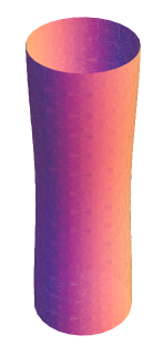
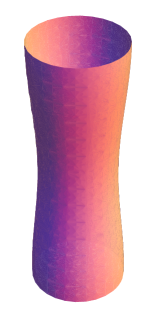
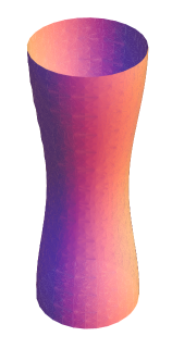
Figure 1: (Colour online) Fermi surfaces for three different values of $b=\frac{v^{\prime}_{F}}{v_{F}}$. The surface in c) has the largest value of $b$.

A gap function with $B_{2g}$ symmetry has line nodes along $k_{x}=0$ and $k_{y}=0$. The Fermi momenta along these nodes (parametrised by $k_{z}$) are

$${\bm{k}}_{F1,3} = (0,\pm(2m(\varepsilon_{F}-\varepsilon_{F}^{\prime}\cos{ck_{z}}))^{1/2},{k_{F}^{\prime}}\sin{ck_{z}})$$ (2)

$$\approx (0,\pm k_{F},k_{F}^{\prime}\sin ck_{z})$$

$${\bm{k}}_{F2,4} = (\pm(2m(\varepsilon_{F}-\varepsilon_{F}^{\prime}\cos{ck_{z}}))^{1/2},0,k_{F}^{\prime}\sin{ck_{z}})$$ (3)

$$\approx (\pm k_{F},0,k_{F}^{\prime}\sin ck_{z}).$$

The magnetic field rotates in the $xy$ plane with an angle $\epsilon$ with respect to the $x$ axis,

$${\bm{H}}=H(\cos{\epsilon},\sin{\epsilon},0).$$ (4)

The supercurrent circulates perpendicular to the field as a function of the distance $r$ from the vortex core and winding angle $\beta$,

$${\bm{v}_{s}}(\bm{r})=\frac{1}{2mr}(-\sin{\epsilon}\cos{\beta},\cos{\epsilon}\cos{\beta},\sin{\beta}).$$ (5)

The Doppler shifts associated with each line node are $\alpha_{i}(\bm{r})={\bm{k}}_{Fi}\cdot{\bm{v}}_{s}$,

$$\alpha_{1,3}(\bm{r}) = =\frac{1}{2mr}[\pm k_{F}\cos{\epsilon}\cos{\beta}+k_{F}^{\prime}\sin{\beta}\sin{ck_{z}}]$$ (6)

$$\alpha_{2,4}(\bm{r}) = =\frac{1}{2mr}[\mp k_{F}\sin{\epsilon}\cos{\beta}+k_{F}^{\prime}\sin{\beta}\sin{ck_{z}}]$$ (7)

II Density of states

In the semi-classical treatment, the argument of the Green’s function $i\omega_{n}$ is replaced by $i\omega_{n}+\alpha$ where $\alpha$ is the Doppler shift. The quasiparticle energy is $E(\bm{k})=\sqrt{\varepsilon^{2}(\bm{k})+\Delta^{2}(\bm{k})}$ which is $\approx\sqrt{v_{F}^{2}k_{1}^{2}+v_{g}^{2}k_{2}^{2}}$ in the vicinity of a node.durst2000 Here $k_{1}$ points in the direction of the node, $k_{2}$ is perpendicular to $k_{1}$ in the $xy$ plane, and the gap velocity is $v_{g}=\partial\Delta/\partial k_{2}|_{\rm node}$. In the vicinity of the $j$th node, the Green’s function takes the form

$$G(\bm{k},i{\tilde{\omega}}_{n},{\bm{r}})=\frac{i{\tilde{\omega}}_{n}+\alpha_{j}(\bm{r})+v_{F}k_{1}}{(i{\tilde{\omega}}_{n}+\alpha_{j}(\bm{r}))^{2}+v_{F}^{2}k_{1}^{2}+v_{g}^{2}k_{2}^{2}}$$ (8)

where $i{\tilde{\omega}}_{n}=i\omega_{n}+i\Gamma_{0}$ and $\Gamma_{0}$ is the scattering rate at zero energy. The density of states is

$$N(\omega,\bm{r})=-\frac{1}{\pi}\sum_{\bm{k}}\Im{G(\bm{k},\tilde{\omega},\bm{r})}.$$ (9)

We divide the volume of integration into four curved cylinder-shaped volumes, each centred around a line node on the Fermi surfacedurst2000 and perform the integration across the disk spanned by $k_{1}$ and $k_{2}$

$$N(0,\bm{r}) = \frac{\Gamma_{0}}{4\pi^{3}v_{F}v_{g}}\sum_{j=1}^{4}\int_{-\pi/c}^{\pi/c}dk_{z}$$

$$\times\left[\ln\frac{p_{0}}{\sqrt{\alpha_{j}^{2}(\bm{r})+\Gamma_{0}^{2}}}+\frac{\alpha_{j}(\bm{r})}{\Gamma_{0}}\tan^{-1}\frac{\alpha_{j}(\bm{r})}{\Gamma_{0}}\right]$$

where $p_{0}$ is the integration cut-off. In the clean limit $|\alpha_{j}/\Gamma_{0}|\gg 1$ the density of states is

$$N(0,\bm{r}) = \frac{1}{4\pi^{3}v_{F}v_{g}}\int_{-\pi/c}^{\pi/c}dk_{z}(|\alpha_{1}(\bm{r})|+|\alpha_{2}(\bm{r})|$$ (11)

$$+|\alpha_{3}(\bm{r})|+|\alpha_{4}(\bm{r})|).$$

Averaging over the vortex cross-section, we obtain

$$\left<N(0,\bm{r})\right>_{H} = \frac{1}{4\pi^{3}v_{F}v_{g}}\frac{1}{\pi R^{2}}\int_{\xi_{0}}^{R}drr\int_{0}^{2\pi}d\beta\int_{-\pi/c}^{\pi/c}dk_{z}$$

$$\times(|\alpha_{1}(\bm{r})|+|\alpha_{2}(\bm{r})|+|\alpha_{3}(\bm{r})|+|\alpha_{4}(\bm{r})|).$$

This leads to the result

$$\left<N(0,\bm{r})\right>_{H} \approx \frac{8}{\pi^{3}v_{g}c}\frac{1}{\pi R}\bigg{[}\sqrt{b^{2}+C^{2}}E\left(\frac{b^{2}}{b^{2}+C^{2}}\right)$$ (13)

$$+\sqrt{b^{2}+S^{2}}E\left(\frac{b^{2}}{b^{2}+S^{2}}\right)\bigg{]}$$

where $b=v_{F}^{\prime}/v_{F}$, $c$ is the lattice constant in the $c$ direction, $C=\cos\epsilon$, $S=\sin\epsilon$ and $E$ is the complete elliptic integral of the second kind. Using $N_{F}\sim 1/cv_{g}\xi_{0}$ and $\xi_{0}/R\sim\sqrt{H/H_{c2}}$, we find

$$\left<N(0,\bm{r})\right>_{H} \sim N_{F}\sqrt{\frac{H}{H_{c2}}}\bigg{[}\sqrt{b^{2}+C^{2}}E\left(\frac{b^{2}}{b^{2}+C^{2}}\right)$$ (14)

$$+\sqrt{b^{2}+S^{2}}E\left(\frac{b^{2}}{b^{2}+S^{2}}\right)\bigg{]}.$$

This function is shown in Fig. 2 for various values of $b$. It is seen that deviations from the perfectly 2D cylindrical Fermi surface leads to a softening of the cusps in the density of states.

Figure 2: Clean limit density of states (the dimensionless expression in the square brackets of Eq. 14) as a function of rotating field angle $\epsilon$ (in radians) for $b=0.02$, $0.05$ and $0.10$.

In the dirty limit $|\alpha_{j}/\Gamma_{0}|\ll 1$ we get

$$\left<N(0,\bm{r})\right>_{H} = \frac{\Gamma_{0}}{4\pi^{3}v_{F}v_{g}}\frac{1}{\pi R^{2}}\int_{\xi_{0}}^{R}drr\int_{0}^{2\pi}d\beta\int_{-\pi/c}^{\pi/c}dk_{z}$$

$$\times \left(4\ln\frac{p_{0}}{\Gamma_{0}}+\frac{\alpha_{1}^{2}(\bm{r})}{\Gamma_{0}^{2}}+\frac{\alpha_{2}^{2}(\bm{r})}{\Gamma_{0}^{2}}+\frac{\alpha_{3}^{2}(\bm{r})}{\Gamma_{0}^{2}}+\frac{\alpha_{4}^{2}(\bm{r})}{\Gamma_{0}^{2}}\right)$$

which produces no oscillations with respect to the rotating field.

III Thermal conductivity

The thermal conductivity tensor is given by the Kubo formula, which is expressed in terms of the imaginary part of the Green’s function as

$$\frac{\widetilde{\kappa}(0,{\bm{r}})}{T}=\frac{k_{B}^{2}}{3}\sum_{\bm{k}}{\bm{v}}_{F}{\bm{v}}_{F}\ {\rm Tr}[\Im\widetilde{G}_{ret}(0,{\bm{r}})\Im\widetilde{G}_{ret}(0,{\bm{r}})],$$ (16)

where $k_{B}$ is the Boltzmann constant and ${\bm{v}_{F}}$ is the Fermi velocity in the direction of ${\bm{k}}$. By again dividing the volume of integration into four regions and introducing the integration variable $p=\sqrt{v_{F}^{2}k_{1}^{2}+v_{g}^{2}k_{2}^{2}}$ we find

$$\frac{\tilde{\kappa}(0,\bm{r})}{T} = \frac{k_{B}^{2}}{3}\frac{1}{(2\pi^{3})v_{F}v_{g}}\int_{0}^{2\pi}d\phi\int_{0}^{p_{0}}dp\,p\int_{-\pi/c}^{\pi/c}dk_{z}$$ (18)

$$\times\sum_{j=1}^{4}({\bm{v}}_{F}{\bm{v}}_{F})_{j}\frac{2\Gamma_{0}^{2}}{[(\alpha_{j}(\bm{r})+p)^{2}+\Gamma_{0}^{2}]^{2}}$$

$$= \frac{k_{B}^{2}}{6\pi^{2}v_{F}v_{g}}\int_{-\pi/c}^{\pi/c}dk_{z}\sum_{j=1}^{4}({\bm{v}}_{F}{\bm{v}}_{F})_{j}$$

$$\times\left(1+\frac{\alpha_{j}(\bm{r})}{\Gamma_{0}}\left(\tan^{-1}\frac{\alpha_{j}(\bm{r})}{\Gamma_{0}}-\frac{\pi}{2}\right)\right)$$

Using (2, 3), in zero magnetic field we get

$$\frac{\tilde{\kappa}(0,0)}{T} = \frac{2k_{B}^{2}v_{F}}{3\pi cv_{g}}\left(\begin{tabular}[]{lclclc}1&&0&0\\ 0&&1&0\\ 0&&0&$(\frac{v_{F}^{\prime}}{v_{F}})^{2}$\end{tabular}\right).$$ (22)

In a finite magnetic field, terms linear in the Doppler shift will vanish upon integration. So the magnetic part of the thermal conductivity is

$$\frac{\delta\tilde{\kappa}(0,\bm{r})}{T} = \frac{k_{B}^{2}}{6\pi^{2}v_{F}v_{g}}\int_{-\pi/c}^{\pi/c}dk_{z}\sum_{j=1}^{4}({\bm{v}}_{F}{\bm{v}}_{F})_{j}$$ (23)

$$\frac{\alpha_{j}(\bm{r})}{\Gamma_{0}}\tan^{-1}\frac{\alpha_{j}(\bm{r})}{\Gamma_{0}}$$

In the clean limit, this reduces to

$$\frac{\delta\tilde{\kappa}(0,\bm{r})}{T} = \frac{k_{B}^{2}}{12\pi v_{F}v_{g}}\int_{-\pi/c}^{\pi/c}dk_{z}\sum_{j=1}^{4}({\bm{v}}_{F}{\bm{v}}_{F})_{j}\frac{|\alpha_{j}(\bm{r})|}{\Gamma_{0}}.$$

The integrand is

$$\frac{v_{F}^{2}}{\Gamma_{0}}\left(\begin{array}[]{ccc}|\alpha_{2}|+|\alpha_{4}|&0&\frac{v_{F}^{\prime}}{v_{F}}(|\alpha_{2}|-|\alpha_{4}|)\sin{ck_{z}}\\ 0&|\alpha_{1}|+|\alpha_{3}|&\frac{v_{F}^{\prime}}{v_{F}}(|\alpha_{1}|-|\alpha_{3}|)\\ \frac{v_{F}^{\prime}}{v_{F}}(|\alpha_{2}|-|\alpha_{4}|)\sin{ck_{z}}&\frac{v_{F}^{\prime}}{v_{F}}(|\alpha_{1}|-|\alpha_{3}|)\sin{ck_{z}}&(\frac{v_{F}^{\prime}}{v_{F}})^{2}(|\alpha_{1}|+|\alpha_{2}|+|\alpha_{3}|+|\alpha_{4}|)\sin^{2}{ck_{z}}\end{array}\right).$$ (25)

The off-diagonal components vanish in the vortex average, and the diagonal components are

$$\frac{\langle\delta\kappa_{xx}\rangle_{H}}{T} = \frac{4}{3\pi^{2}}\frac{k_{B}^{2}}{R\Gamma_{0}}\frac{v_{F}^{2}}{v_{g}c}\sqrt{b^{2}+S^{2}}E\left(\frac{b^{2}}{b^{2}+S^{2}}\right)$$ (26)

$$\frac{\langle\delta\kappa_{yy}\rangle_{H}}{T} = \frac{4}{3\pi^{2}}\frac{k_{B}^{2}}{R\Gamma_{0}}\frac{v_{F}^{2}}{v_{g}c}\sqrt{b^{2}+C^{2}}E\left(\frac{b^{2}}{b^{2}+C^{2}}\right)$$ (27)

$$\frac{\langle\delta\kappa_{zz}\rangle_{H}}{T} = \frac{4}{9\pi^{2}}\frac{k_{B}^{2}}{R\Gamma_{0}}\frac{v_{F}^{2}}{v_{g}c}\left(\sqrt{b^{2}+S^{2}}\left[-S^{2}K\left(\frac{b^{2}}{S^{2}+b^{2}}\right)\right.\right.$$ (28)

$$\hskip 50.58878pt\left.+(2b^{2}+S^{2})E\left(\frac{b^{2}}{S^{2}+b^{2}}\right)\right]$$

$$\hskip 28.90755pt+\sqrt{b^{2}+C^{2}}\left[-C^{2}K\left(\frac{b^{2}}{C^{2}+b^{2}}\right)\right.$$

$$\hskip 50.58878pt\left.\left.+(2b^{2}+C^{2})E\left(\frac{b^{2}}{C^{2}+b^{2}}\right)\right]\right)$$

where $K$ is the complete elliptic integral of the first kind. $\kappa_{zz}$ is plotted in Fig. 3 for different values of $b$. In the limit $b\rightarrow 0$ the cusps are sharp, however the oscillation amplitude goes to zero. The oscillation amplitude increases exponentially with $b$.

Figure 3: Clean limit thermal conductivity $\kappa_{zz}$ (the dimensional expression in the round brackets of Eq. 28) as a function of rotating field angle $\epsilon$ (in radians) for $b=0.02$, $0.05$ and $0.10$.

In the dirty limit, (23) reduces to

$$\frac{\delta\tilde{\kappa}(0,\bm{r})}{T} = \frac{k_{B}^{2}}{6\pi^{2}v_{F}v_{g}}\int_{-\pi/c}^{\pi/c}dk_{z}\sum_{j=1}^{4}({\bm{v}}_{F}{\bm{v}}_{F})_{j}\frac{\alpha_{j}^{2}(\bm{r})}{\Gamma_{0}^{2}}$$

Again, the off-diagonal components vanish in the vortex average, and the diagonal elements are

$$\left\langle\frac{\delta\kappa_{xx}(0,\bm{r})}{T}\right\rangle_{H} = \frac{k_{B}^{2}v_{F}^{3}}{12\pi v_{g}}\log(R/\xi_{0})(2C^{2}+b^{2})$$ (30)

$$\left\langle\frac{\delta\kappa_{yy}(0,\bm{r})}{T}\right\rangle_{H} = \frac{k_{B}^{2}v_{F}^{3}}{12\pi v_{g}}\log(R/\xi_{0})(2S^{2}+b^{2})$$ (31)

$$\left\langle\frac{\delta\kappa_{zz}(0,\bm{r})}{T}\right\rangle_{H} = \frac{k_{B}^{2}v_{F}^{3}}{12\pi v_{g}}\log(R/\xi_{0})(1+3b^{2}/2)$$ (32)

Similar to the dirty limit density of states (LABEL:dirtyDOS), there are no rotating field-dependent oscillations in the dirty limit of $\kappa_{zz}$.

IV Discussion and Conclusions

The topology of the true Fermi surface of YNi₂B₂C shown in Ref. yamaguchi2004, is difficult to discern, however the validity of our calculation only requires that the Fermi surface exists at the positions of the nodes and spans all or most of the Brillioun zone in the $c$ direction with a slight curvature characterised by the parameter $b$. The main point is that the cusp features observed in the field angle-dependent heat capacitypark2003 are a feature of line nodes and the cusp features observed in the field angle-dependent thermal conductivity are a feature of line nodes on a quasi-2D Fermi surface. In contrast, the semi-classical (Doppler shift) treatment of point nodes (which may not even be valid) is insensitive to Fermi surface topology and produces neither cusp features nor four-fold oscillations.tayseer2008

Using $R\approx 4\times 10^{-8}$ m (for a 1 T field), $T=0.56$ K, $E_{F}=9$ Ry,yamaguchi2004 $v_{F}\approx 3\times 10^{7}$ m/s, gap maximum $\Delta_{0}=v_{g}\hbar k_{F}=30$ K and scattering rate $\Gamma_{0}=1$ K leads to an estimate of the prefactor in (28) of $\frac{4T}{9\pi^{2}}\frac{k_{B}^{2}}{R\Gamma_{0}}\frac{v_{F}^{2}}{v_{g}c}\approx 10^{4}$ W/Km. The experimentally observed oscillation amplitude is $\approx 2\times 10^{-3}$. Comparing with the oscillation amplitudes shown in Fig. 3, one may deduce that the value of $b$ is approximately 0.02. Such a small value of $b$ produces sharp cusps in the field angle-dependent $\kappa_{zz}$ oscillations and is therefore fully consistent with experiment.

Thus the most straight-forward model that best describes accumulated observations on YNi₂B₂C is that the superconducting order parameter is $\Delta\sim k_{x}k_{y}$, which belongs to the irreducible representation $B_{2g}$ of the point group $D_{4h}$, with associated line nodes along $k_{x}=0$ and $k_{y}=0$.

References

• (1) K. Izawa, K. Kamata, Y. Nakajima, Y. Matsuda, T. Watanabe, M. Nohara, H. Takagi, P. Thalmeier and K. Maki, Phys.Β Rev.Β Lett. 89, 137006 (2002).
• (2) R. J. Cava, H. Takagi, H. W. Zandbergen, J. J. Krajewski, W. F. Peck Jr., T. Sigrist, B. Batlogg, R. B. van Dover, R. J. Felder, K. Mizuhashi, J. O. Lee, H. Eisaki and S. Uchida, Nature 367, 252 (1994).
• (3) C. Godart, L. C. Gupta, R. Nagarajan, S. K. Dhar, H. Noel, M. Potel, C. Mazumdar, Z. Hossain, C. Levy-Clement, G. Schiffmacher, B. D. Padalia and R. Vijayaraghavan, Phys.Β Rev.Β B 51, 489 (1995).
• (4) M. Nohara, M. Isshiki, F. Sakai and H. Takagi, J. Phys.Β Soc.Β Jpn. 68, 1078 (1999); M. Nohara, H. Suzuki, N. Mangkorntong and H. Takagi, Physica C 341-348, 2177 (2000).
• (5) K. Izawa, H. Yamaguchi, Y. Matsuda, H. Shishido, R. Settai and Y. Onuki, Phys.Β Rev.Β Lett. 87, 057002 (2001).
• (6) G.-Q. Zheng, Y. Wada, K. Hashimoto, Y. Kitaoka, K. Asayama, H. Takeya and K. Kadowaki, J. Phys.Β Chem.Β Solids 59, 2169 (1998).
• (7) I.-S. Yang, M. V. Klein, S. L. Cooper, P. C. Canfield, B. K. Cho and S.-I. Lee, Phys.Β Rev.Β B 62, 1291 (2000).
• (8) G. E. Volovik and L. P. Gor’kov, Sov.Β Phys.Β JETP 61, 843 (1985).
• (9) M. Sigrist and K. Ueda, Rev.Β Mod.Β Phys. 63, 239 (1991).
• (10) T. Park, M. B. Salamon, E. M. Choi, H. J. Kim and S.-I. Lee, Phys.Β Rev.Β Lett. 90, 177001 (2003).
• (11) Y. Matsuda, K. Izawa and I. Vekhter, J. Phys.: Condens.Β Matter 18, R705 (2006).
• (12) T. Siegrist, Nature 367, 254 (1994).
• (13) J. I. Lee, T. S. Zhao, I. G. Kim, B. I. Min and S. J. Youn, Phys.Β Rev.Β B 50, 4030 (1994).
• (14) D. J. Singh, Solid State Commun. 98, 899 (1996).
• (15) K. Yamaguchi, H. Katayama-Yoshida, A. Yanase and H. Harima, Physica C 412-414, 225 (2004).
• (16) G. E. Volovik, JETP Lett. 58, 471 (1993).
• (17) H. Aubin, K. Behnia, M. Ribault, R. Gagnon and L. Taillefer, Phys.Β Rev.Β Lett. 78, 2624 (1997).
• (18) T. R. Abu Alrub and S. H. Curnoe, Phys.Β Rev.Β B 78, 104521 (2008).
• (19) A. C. Durst and P. A. Lee, Phys. Rev. B 62, 1270 (2000).