Time series analysis Brownian motion Networks and genealogical trees

The Visibility Graph: a new method for estimating the Hurst exponent of fractional Brownian motion

Abstract

Fractional Brownian motion (fBm) has been used as a theoretical framework to study real time series appearing in diverse scientific fields. Because its intrinsic non-stationarity and long range dependence, its characterization via the Hurst parameter $H$ requires sophisticated techniques that often yield ambiguous results. In this work we show that fBm series map into a scale free visibility graph whose degree distribution is a function of $H$. Concretely, it is shown that the exponent of the power law degree distribution depends linearly on $H$. This also applies to fractional Gaussian noises (fGn) and generic $f^{-\beta}$ noises. Taking advantage of these facts, we propose a brand new methodology to quantify long range dependence in these series. Its reliability is confirmed with extensive numerical simulations and analytical developments. Finally, we illustrate this method quantifying the persistent behavior of human gait dynamics.

Self-similar processes such as fractional Brownian motion (fBm) [1] are currently used to model fractal phenomena of different nature, ranging from Physics or Biology to Economics or Engineering. To cite a few, fBm has been used in models of electronic delocalization [2], as a theoretical framework to analyze turbulence data [3], to describe geologic properties [4], to quantify correlations in DNA base sequences [5], to characterize physiological signals such as human heartbeat [6] or gait dynamics [7], to model economic data [8] or to describe network traffic [11, 9, 10]. Fractional Brownian motion $B_{H}(t)$ is a non-stationary random process with stationary self-similar increments (fractional Gaussian noise) that can be characterized by the so called Hurst exponent, $0<H<1$. The one-step memory Brownian motion is obtained for $H=\frac{1}{2}$, whereas time series with $H>\frac{1}{2}$ shows persistence and anti-persistence if $H<\frac{1}{2}$.

While different fBm generators and estimators have been introduced in the last years, the community lacks consensus on which method is best suited for each case. This drawback comes from the fact that fBm formalism is exact in the infinite limit, i.e. when the whole infinite series of data is considered. However, in practice, real time series are finite. Accordingly, long range correlations are partially broken in finite series, and local dynamics corresponding to a particular temporal window are overestimated. The practical simulation and the estimation from real (finite) time series is consequently a major issue that is, hitherto, still open. An overview of different methodologies and comparisons can be found in [11, 12, 13, 14, 15, 16, 17, 18] and references therein.

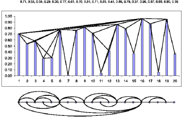
Figure 1: Example of a time series ($20$ data, depicted in the upper part) and the associated graph derived from the visibility algorithm. In the graph, every node corresponds, in the same order, to a series data. The visibility rays between the data define the links connecting nodes in the graph.

Most of the preceding methods operate either on the time domain (e.g. Aggregate Variance Method, Higuchi’s Method, Detrended Fluctuation Analysis, Range Scaled Analysis, etc) or in the frequency or wavelet domain (Periodogram Method, Whittle Estimator, Wavelet Method). In this letter we introduce an alternative and radically different method, the Visibility Algorithm, based in graph theoretical techniques. In a recent paper this new tool for analyzing time series has been presented [19]. In short, a visibility graph is obtained from the mapping of a time series into a network according with the following visibility criterium: two arbitrary data $(t_{a},y_{a})$ and $(t_{b},y_{b})$ in the time series have visibility, and consequently become two connected nodes in the associated graph, if any other data $(t_{c},y_{c})$ such that $t_{a}<t_{c}<t_{b}$ fulfills:

$$y_{c}<y_{b}+(y_{a}-y_{b})\frac{t_{b}-t_{c}}{t_{b}-t_{a}}.$$ (1)

In fig.1 we have represented for illustrative purposes an example of how a given time series maps into a visibility graph by means of the Visibility Algorithm. A preliminary analysis has shown that series structure is inherited in the visibility graph [19]. Accordingly, periodic series map into regular graphs, random series into random graphs and fractal series into scale free graphs [20]. In particular, it was shown that the visibility graph obtained from the well-known Brownian motion has got both the scale-free and the small world properties [19]. Here we show that the visibility graphs derived from generic fBm series are also scale free. This robustness goes further, and we prove that a linear relation between the exponent $\gamma$ of the power law degree distribution in the visibility graph and the Hurst exponent $H$ of the associated fBm series exists. Therefore, the visibility algorithm provides an alternative method to compute the Hurst exponent and then, to characterize fBm processes. This also applies to fractional gaussian noise (fGn) [1] which are nothing but the increments of a fBm, and generic $f^{-\beta}$ noises, enhancing the visibility graph as a method to detect long range dependence in time series.

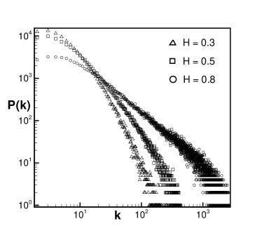
Figure 2: Degree distribution of three visibility graphs, namely (i) triangles: extracted from a fBm series of $10^{5}$ data with $H=0.3$, (ii) squares: extracted from a fBm series of $10^{5}$ data with $H=0.5$, (iii) circles: extracted from a fBm series of $10^{5}$ data with $H=0.8$. Note that distributions are not normalized. The three visibility graphs are scale-free since their degree distributions follow a power law $P(k)\sim k^{-\gamma}$ with decreasing exponents $\gamma_{0.3}>\gamma_{0.5}>\gamma_{0.8}$.

In fig.2 we have depicted in log-log the degree distribution of the visibility graph associated with three artificial fBm series of $10^{5}$ data, namely an anti-persistent series with $H=0.3$ (triangles), a memoryless Brownian motion with $H=0.5$ (squares) and a persistent fBm with $H=0.8$ (circles). As can be seen, these distributions follow a power law $P(k)\sim k^{-\gamma}$ with decreasing exponents $\gamma_{0.3}>\gamma_{0.5}>\gamma_{0.8}$.

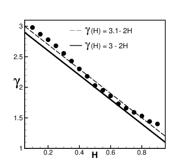
Figure 3: (Black dots) Numerical estimation of exponent $\gamma$ of the visibility graph associated with a fBm series with exponent $H$. In each case $\gamma$ is averaged over $10$ realizations of a fBm series of $10^{4}$ data, in order to avoid non-stationary biases (the error bars are included in the dot size). The dotted line corresponds to the best linear fitting $\gamma(H)=a-bH$, where $a=3.1\pm 0.1$ and $b=2.0\pm 0.1$, and the solid line corresponds to the theoretical prediction $\gamma(H)=3-2H$. Both results are consistent. Note that deviations from the theoretical law take place for values of $H>0.5$ and $H<0.5$ (strongly correlated or anti-correlated series), where fBm generators evidence finite-size accuracy problems [21], these being more acute the more we move away from the non-correlated case $H=0.5$.

In order to compare $\gamma$ and $H$ appropriately, we have calculated the exponent of different scale free visibility graphs associated with fBm artificial series of $10^{4}$ data with $0<H<1$ generated by a wavelet based algorithm [23]. Note at this point that some bias is inevitably present since artificial series generators are obviously not exact, and consequently the nominal Hurst exponents have an associated error [21]. For each value of the Hurst parameter we have thus averaged the results over $10$ realizations of the fBm process. We have estimated exponent $\gamma$ in each case through Maximum Likelihood Estimation (MLE) [25]:

$$\gamma=1+n\bigg{[}\sum_{i=1}^{n}\log\frac{x_{i}}{x_{min}}\bigg{]}^{-1},$$ (2)

where $n$ is total number of values taken into account, $x_{i},\ i=1,..,n$ are the measured values and $x_{min}$ corresponds to the smallest value of $x$ for which the power law behavior holds. In fig.3 we have represented the relation between $\gamma$ and $H$ (black circles). As can be seen, a roughly linear relation holds (the dotted line represents the best linear fitting $\gamma=3.1-2H$).

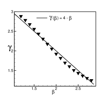
Figure 4: (Black triangles) Numerical estimation of exponent $\gamma$ of the visibility graph associated with a $f^{-\beta}$ noise. In each case $\gamma$ is averaged over $10$ realizations of a $f^{-\beta}$ series of $10^{6}$ data, in order to avoid non-stationary biases (the error bars are included in the triangle size). The straight line corresponds to the theoretical prediction in eq.7.

That fBm yields scale free visibility graphs is not that surprising. The most highly connected nodes (hubs) are the responsible for the heavy tailed degree distributions. Within fBm series, hubs are related to extreme values in the series, since a data with a very large value has typically a large connectivity, according to eq. 1. In order to calculate the tail of the distribution we consequently need to focus on the hubs, and thus calculate the probability that an extreme value has a degree $k$. Suppose that at time $t$ the series reaches an extreme value (a hub) $B_{H}(t)=h$. The probability of this hub to have degree $T$ is

$$P(T)\sim P_{fr}(T)r(T),$$ (3)

where $P_{fr}(T)$ provides the probability that after $T$ time steps, the series returns to the same extreme value, i.e. $B(t+T)=h$ (and consequently the visibility in $t$ gets truncated in $t+T$), and $r(T)$ is the percentage of nodes between $t$ and $t+T$ that $t$ may see. $P_{fr}(T)$ is nothing but the first return time distribution, which is known to scale as $P_{fr}(T)\sim T^{H-2}$ for fBm series [22]. On the other hand, the percentage of visible nodes between two extreme values is related to the roughness of the series in that basin, that is, to the way that a series of $T$ time steps folds. This roughness is encoded in the series standard deviation [1], such that intuitively, we have $r(T)\sim T^{H}/T=T^{H-1}$ (this fact has been confirmed numerically). Finally, notice that in this context $T\equiv k$, so eq.3 converts into

$$P(k)\sim k^{H-2}k^{H-1}=k^{2H-3},$$ (4)

what provides a linear relation between the exponent of the visibility graph degree distribution and the Hurst exponent of the associated fBm series:

$$\gamma(H)=3-2H,$$ (5)

in good agreement with our previous numerical results. Note in figure 3 that numerical results obtained from artificial series deviate from the theoretical prediction for strongly-correlated ones ($H>0.5$ or $H<0.5$). This deviation is related to finite size effects in the generation of finite fBm series [21], and these effects are more acute the more we deviate from the non-correlated case $H=0.5$. In any case, a scatter plot of the theoretical (eq.5) versus the empirical estimation of $\gamma(H)$ provides statistical conformance with a correlation coefficient $c=0.99$.
To check further the consistency of the visibility algorithm, an estimation of the power spectra is performed. It is well known that fBm has a power spectra that behaves as $1/f^{\beta}$, where the exponent $\beta$ is related to the Hurst exponent of an fBm process through the well known relation [24]

$$\beta(H)=1+2H.$$ (6)

Now according to eqs.5 and 6, the degree distribution of the visibility graph corresponding to a time series with $f^{-\beta}$ noise should be again power law $P(k)\sim k^{-\gamma}$ where

$$\gamma(\beta)=4-\beta.$$ (7)

In fig.4 we depict (triangles) the empirical values of $\gamma$ corresponding to $f^{-\beta}$ artificial series of $10^{6}$ data with $\beta$ ranging from $1.2$ to $2.8$ in steps of size $0.1$ [26]. For each value of $\beta$ we have again averaged the results over $10$ realizations and estimated $\beta$ through MLE (eq.2). The straight line corresponds to the theoretical prediction eq.7, showing good agreement with the numerics. In this case, a scatter plot confronting theoretical versus empirical estimation of $\gamma(\beta)$ also provides statistical conformance between them, up to $c=0.99$.
Finally, observe that eq.6 holds for fBm processes, while for the increments of an fBm process, known as a fractional Gaussian noise (fGn), the relation between $\beta$ and $H$ turns to be [24]:

$$\beta(H)=-1+2H,$$ (8)

where $H$ is the Hurst exponent of the associated fBm process. We consequently can deduce that the relation between $\gamma$ and $H$ for a fGn (where fGn is a series composed by the increments of a fBm) is

$$\gamma(H)=5-2H.$$ (9)

Notice that eq.9 can also be deduced applying the same heuristic arguments as for eq.5 with the change $H\rightarrow H-1$.
In order to illustrate this latter case, we finally address a realistic and striking dynamics where long range dependence has been recently described. Gait cycle (the stride interval in human walking rhythm) is a physiological signal that has been shown to display fractal dynamics and long range correlations in healthy young adults [27, 28]. In the upper part of fig.5 we have plotted to series describing the fluctuations of walk rhythm of a young healthy person, for slow pace (bottom series of $3304$ points) and fast pace (up series of $3595$ points) respectively (data available in www.physionet.org/physiobank/database/umwdb/ [29]). In the bottom part we have represented the degree distribution of their visibility graphs. These ones are again power laws with exponents $\gamma=3.03\pm 0.05$ for fast pace and $\gamma=3.19\pm 0.05$ for slow pace (derived through MLE). According to eq.7, the visibility algorithm predicts that gait dynamics evidence $f^{-\beta}$ behavior with $\beta=1$ for fast pace, and $\beta=0.8$ for slow pace, in perfect agreement with previous results based on a Detrended Fluctuation Analysis [27, 28]. These series record the fluctuations of walk rhythm (that is, the increments), so according to eq.9, the Hurst exponent is $H=1$ for fast pace and $H=0.9$ for slow pace, that is to say, dynamics evidences long range dependence (persistence) [27, 28].

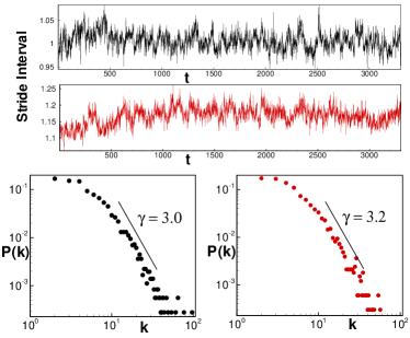
Figure 5: Black signal: time series of $3595$ points from the stride interval of a healthy person in fast pace. Red signal: time series of $3304$ points from the stride interval of a healthy person in slow pace. Bottom: Degree distribution of the associated visibility graphs (the plot is in log-log). These are power laws where $\gamma=3.03\pm 0.05$ for the fast movement (black dots) and $\gamma=3.19\pm 0.05$ for the slow movement (red dots), what provides $\beta=1$ and $\beta=0.8$ for fast and slow pace respectively according to eq.7, in agreement with previous results [27, 28].

As a summary, the visibility graph is an algorithm that map a time series into a graph. In so doing, classic methods of complex network analysis can be applied to characterize time series from a brand new viewpoint [19]. In this work we have pointed out how graph theory techniques can provide an alternative method to quantify long range dependence and fractality in time series. We have reported analytical and numerical evidences showing that the visibility graph associated to a generic fractal series with Hurst exponent $H$ is a scale free graph, whose degree distribution follows a power law $P(k)\sim k^{-\gamma}$ such that: (i) There is a universal relation between $\gamma$ and the exponent $\beta$ of its power spectrum that reads $\gamma=4-\beta$; (ii) for fBm signals (where $H$ is defined such that $\beta(H)=1+2H$), the relation between $\gamma$ and H reads $H(\gamma)=\frac{3-\gamma}{2}$ while for fGn signals (the increments of a fBm where H is defined as $\beta(H)=-1+2H$), we have $H(\gamma)=\frac{5-\gamma}{2}$.
The reliability of this methodology has been confirmed with extensive simulations of artificial fractal series and real (small) series concerning gait dynamics. To our knowledge, this is the first method for estimation of long range dependence in time series based in graph theoretical techniques advanced so far. Some questions concerning its accuracy, flexibility and computational efficiency will be at the core of further investigations. In any case, we do not pretend in this work to compare its accuracy with other estimators, but to propose an alternative and simple method based in completely different techniques with potentially broad applications.

- [1] B.B Mandelbrot and J.W Van Ness, SIAM Review 10, 4 (1968) 422-437.
- [2] F.A.B.F. de Moura and M.L. Lyra, Phys. Rev. Lett. 81, 17 (1998).
- [3] J.F. Muzy, E. Bacry and A. Arneodo, Phys. Rev. Lett. 67, 25 (1991); K. Kiyani et al., ibid. 98, 2111101 (2007).
- [4] M.P. Golombek et al., Nature 436, 44-48 (2005).
- [5] R.F. Voss, Phys. Rev. Lett. 68, 25 (1992).
- [6] P.Ch. Ivanov et al., Nature 399, 461-465 (1999).
- [7] J. Haussdorf, Human Movement Review 26 (2007) 555-589.
- [8] J.A.O. Matos et al., Physica A 387, 15 (2008) 3910-3915.
- [9] W.E. Leland et al., IEEE/ACM Transactions on Networking 2 (1994) 1-15.
- [10] T. Mikosch et al. The Annals of Applied Probability , 12, 1 (2002) 23 68.
- [11] T. Karagiannis, M. Molle and M. Faloutsos, IEEE internet computing 8, 5 (2004) 57-64.
- [12] R. Weron, Physica A 312 (2002) 285-299.
- [13] B. Pilgram and D.T. Kaplan, Physica D 114 (1998) 108-112.
- [14] J. W. Kantelhardt, Fractal and multifractal time series, in: Springer encyclopaedia of complexity and system science (in press, 2008) preprint arXiv:0804.0747.
- [15] B. Podobnik, H.E. Stanley, Phys. Rev. Lett. 100, 084102 (2008).
- [16] A. Carbone, Phys. Rev. E 76, 056703 (2007).
- [17] J. Mielniczuk and P. Wojdyllo, Comput. Statist. Data Anal. 51 (2007) 4510-4525.
- [18] I. Simonsen, A. Hansen and O.M. Nes, Phys. Rev. E 58, 3 (1998).
- [19] L. Lacasa, B. Luque, F. Ballesteros, J. Luque and J.C. Nuño, Proc. Natl. Acad. Sci. USA 105, 13 (2008), 4972-4975.
- [20] R. Albert and A.L. Barabasi, Rev. Mod. Phys. 74, 47 (2002).
- [21] G.A. Horn et al. Perfomance Evaluation 64, 2 (2007) 162-190.
- [22] M. Ding and W. Yang, Phys. Rev. E, 52, 1 (1995).
- [23] P. Abry and F. Sellan, Appl. and Comp. Harmonic Anal., 3, 4 (1996) 377-383.
- [24] P.S. Adison, Fractal and Chaos: an illustrative course. IOP Publishing Ltd (1997).
- [25] M.E.J. Newmann, Contemporary Physics 46, 5 (2005), 323-351.
- [26] The series have been generated by a method where each frequency component have a magnitude generated from a Gaussian white process and scaled by the appropriate power of the frequency. The phase is uniformly distributed on . See http://local.wasp.uwa.edu.au/pbourke/fractals/noise/ for a source code.
- [27] A.R. Goldenberger et al., Proc. Natl. Acad. Sci. USA 99, 1 (2002), 2466-2472.
- [28] J.M. Hausdorff et al., J. App. Physiol. 80 (1996) 1448-1457.
- [29] A.L. Goldberger et al., Circulation 101, 23 (2000) 215-220.