Computation of Resistive Wakefields

Abstract

We evaluate longitudinal resistive wakefields for cylindrical beam pipes numerically and compare the results with existing approximate formulæ. We consider an ultra-relativistic bunch traversing a cylindrical, metallic tube for a model in which the wall conductivity is taken to be first independent and second dependent on frequency, and we show how these can be included simply and efficiently in particle tracking simulations. We also extend this to higher order modes, and to the transverse wakes. This full treatment can be necessary in the design of modern nano-beam accelerators.

I Introduction

The requirements of modern accelerators are placing increasing demands on technology, with small precisely-defined beam bunches passing through physically small beam pipes and collimators. This means that the effects of wakefields produced by induced charges and currents are becoming increasingly important and require accurate calculation to ensure they do not dilute the emittance of the beam.

The wakefields from particles in a bunch may affect other particles in the same bunch (intrabunch wakes) and also particles in subsequent bunches (interbunch wakes). For physically small apertures the effects of short-range intra bunch forces become important and need to be considered, as well as the more familiar long range interbunch effects.

For a relativistic particle in a perfectly conducting uniform beam pipe the wake is zero. For a non-uniform beam pipe of finite conductivity the effect is thus separated into geometric and resistive wakes, the second of which is considered here.

The wake is due to the Lorentz force $\vec{F}=q(\vec{E}+~{}\vec{v}\wedge\vec{B})$, however for the longitudinal component $F_{\parallel}$ the second term is zero and only $E_{\parallel}$ need be considered. For a purely resistive wake, the wake field, $\vec{E}+~{}\vec{v}\wedge\vec{B}$, is constant and the integrated effect of the complete transit of the bunch through a section of pipe, generally called the wake potential, is obtained just by multiplying the wake field by the pipe length. The wake field is found Chao (1993) by writing down Maxwell’s Equations in the beam aperture and in the beam pipe and matching them subject to appropriate boundary conditions. These solutions can be written as a sum over angular modes. For many purposes only the knowledge of the leading modes ($m=0$ and $m=1$) is adequate, however as requirements become more stringent a technique is needed that will work in the general case.

Finding solutions of Maxwell’s equations is more readily done in frequency (or wavenumber) space rather than physical space, as differentiation becomes multiplication. The Fourier Transform of the wake is the impedance

$$\tilde{\vec{F}}(k)=\int\vec{F}(s)e^{iks}ds\qquad\vec{F}(s)={1\over 2\pi}\int\tilde{\vec{F}}(k)e^{-iks}dk$$ (1)

where $s$ is the distance along the beam axis between a leading particle which creates the field and a trailing (witness) particle which feels the effect.

For many purposes a knowledge of the impedance suffices. The ‘kick factor’ averaged over all the bunch is also often useful and expressions are given in the literature. However the kick factor only gives the mean effect for the whole bunch and in particle tracking codes an expression is needed for the physical impulse that one leading particle has on another trailing particle. Existing approaches use expressions in different regimes Latina and et al. (2006), where the division is somewhat arbitrary. We have found an approach which unifies, simplifies and speeds up the calculations, and makes the underlying physics clear. It includes short range and long range wakes with no artificial division between them. It can also be extended to arbitrary angular order.

Chao Chao (1993) gives a general formula for the impedance, from which he obtains an expression for the physical wake which is valid in the long-range limit. Bane and Sands Bane (1991); Bane and Sands (1995) extend this to shorter range though still making approximations.

Gluckstern, van Zeits and ZotterGluckstern et al. (1993) consider resistive wakefields for circular, elliptical and rectangular pipes, but they only evaluate the impedance, not the physical wake, and only consider the lowest ($m$=0 longitudinal, $m=1$ transverse) modes. Yokoya Yokoya (1993) also considers beam pipes of general cross section, though his results are self-admittedly complicated and not easy to implement. Lutman, Vescovi and Craievich Lutman et al. (2008) generalise the results to elliptical beam pipes, including circular and planar apertures as special cases. Although a very general approach, they consider only leading modes and the examples they give are specific and not directly applicable to simulation programs.

II The longitudinal wake for $m=0$

The Fourier Transform of the $m=0$ mode of the longitudinal component of the wakefield is given by Bane (1991)

$$\tilde{E}_{z}(k)={2q\over b}{1\over{ikb\over 2}-\left({\lambda\over k}+{k\over\lambda}\right)\left(1+{i\over 2\lambda b}\right)}$$ (2)

where

$$\lambda(k)=\sqrt{2\pi\sigma|k|\over c}(i+sgn(k))$$ (3)

with $q$ the charge of the particle, $b$ the radius of the tube, $\sigma$ the conductivity of the pipe, and $c$ the speed of light. This assumes axial symmetry, the validity of Ohm’s law, relativistic particles, and that the skindepth is smaller than both the thickness of the pipe and the tube radius, but is otherwise general. This enables the Bessel function solution of $\tilde{\vec{F}}(k)$ to be replaced by a sinusoidal form, i.e. the asymptotic form of $J_{0}(x)\propto x^{-1/2}e^{ix}$, as suggested by Chao(Chao (1993),p.43), which leads to the $\left(\frac{i}{2\lambda b}\right)$ term in the Equation 2.

It is convenient to introduce $s_{0}$, the scaling length

$$s_{0}=\root 3 \of{cb^{2}\over 2\pi\sigma}$$ (4)

and thus the dimensionless quantities $K$, the scaled wave number and $s^{\prime}$, the scaled length

$$K=s_{0}k$$ (5)

$$s^{\prime}={s\over s_{0}}$$ (6)

It is useful to note that

$$\lambda=\frac{b\sqrt{|K|}}{s_{0}^{2}}(1\pm i)\qquad\frac{k}{\lambda}=\frac{1}{2}\frac{s_{0}\sqrt{|K|}}{b}(1\mp i)$$

$$\frac{\lambda}{k}=\frac{b}{s_{0}\sqrt{|K|}}(1\pm i)$$ (7)

where the upper sign applies for positive $k$, the lower for negative $k$.

To find the corresponding wakefield requires the inverse Fourier transform. This has been much studied in the literatureBane (1991); Chao (1993), using various approximations forms of Equation 2 and evaluating them by a contour integral. By contrast we will do the integration numerically, enabling us to provide a general technique without making approximations as has been done previously Chao (1993); Bane and Sands (1995); Latina and et al. (2006) and to evaluate the different regions wherein such approximations are valid.

The back transform can be written

$${E}_{z}(s)=\frac{1}{2\pi}\int_{-\infty}^{\infty}\Bigl{(}Re[f_{even}(k)]\cos(ks)$$

$$+Im[f_{odd}(k)]\sin(ks)\Bigr{)}dk$$ (8)

$${E}_{z}(s)=\frac{s_{0}}{2\pi}\int_{-\infty}^{\infty}\Bigl{(}Re[f_{even}(K)]\cos(Ks^{\prime})$$

$$+Im[f_{odd}(K)]\sin(Ks^{\prime})\Bigr{)}dK$$ (9)

where the functions are the even and odd parts of $\tilde{E}_{z}(k)$. This separation is necessary to avoid problems with the alternating signs and the modulus operations in Equations 7.

II.1 The first order approximation

In the limit of large $b$ compared to $s_{0}$ and neglecting high and low frequencies Equation 2 can be approximated by

$$\tilde{E}_{z}(k)=-{2qk\over\lambda b}$$ (10)

The Fourier Transform is given by Chao Chao (1993) as

$$E_{z}(s)={q\over 2\pi b}\sqrt{c\over\sigma}s^{-{3\over 2}}.$$ (11)

However we can also evaluate it numerically, in preparation for more complicated forms of $\tilde{E}_{z}(k)$. We have

$$f_{even}(K) = \frac{1}{2}\Bigl{[}f(K)+f(-K)\Bigl{]}=-\sqrt{K},$$

$$f_{odd}(K) = \frac{1}{2}\Bigl{[}f(K)-f(-K)\Bigl{]}=i\sqrt{K}$$ (12)

where the functions are the even and odd parts of $\tilde{E}_{z}(k)$, having taken out a common factor of ${q\over b^{2}}$. The even part is purely real and the odd part is purely imaginary, as they must be.

A function like $\sqrt{K}\sin(K)$ presents problems for numerical integrals as the function is oscillating with increasing amplitude, and any summation technique (trapezoidal rule, Simpson’s rule or Gaussian quadrature) will not work. However we know that the integral exists because it can be done analytically. We can perform the $K$ integral by first integrating with respect to $s^{\prime}$, thereby dividing by a factor of $K$ so that the oscillations decrease in size and the numerical integration can succeed

$$\int_{0}^{s}E_{z}(x)dx = s_{0}\int_{0}^{s/s_{0}}E_{z}(x^{\prime})dx^{\prime}$$ (13)

$$= {s_{0}q\over\pi b^{2}}\int_{0}^{\infty}\Bigl{(}\frac{Re[f_{even}(K)]}{K}\sin{(Ks^{\prime})}$$

$$- \frac{Im[f_{odd}(K)]}{K}\cos{(Ks^{\prime})}\Bigr{)}dK$$

The result can then be differentiated numerically, using an intermediate interpolating function, to give the desired wakefield.

This can be verified and results are shown in Fig. 1, for $b=1$ cm and $\sigma=5.8\times 10^{7}\,(\Omega m)^{-1}$. These results are indistinguishable from those obtained by plotting Chao’s formula, Equation 11.

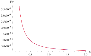
Figure 1: The long range wake given by Equation 13 and Equation 11 Chao (1993).

II.2 A more accurate formula

If the large $s$ requirement is relaxed then a second term has to be included in the denominator and Equation 2 is approximated by

$$\tilde{E}_{z}(k)=\frac{2q}{b}\frac{1}{\frac{ikb}{2}-\frac{\lambda}{k}}$$ (14)

The even and odd parts are

$$f_{even}(K) = -\frac{\frac{2}{\sqrt{K}}}{\Bigl{(}\frac{K}{2}-\frac{1}{\sqrt{K}}\Bigr{)}^{2}+\frac{1}{K}},$$

$$f_{odd}(K) = -\frac{2i\Bigl{(}\frac{K}{2}-\frac{1}{\sqrt{K}}\Bigr{)}}{\Bigl{(}\frac{K}{2}-\frac{1}{\sqrt{K}}\Bigr{)}^{2}+\frac{1}{K}}$$ (15)

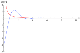
Figure 2: The longitudinal wake in the second approximation (blue line) with the long range form (red line) for comparison.

Although the wake is a function of three parameters ($s,b$ and $\sigma$), the use of the scaling length $s_{0}$ enables it to be written as a universal function $U(s^{\prime})$, where $E_{z}(s,b)=~{}{s_{0}q\over b^{2}}U(s/s_{0})$. The result is shown in Fig. 2, together with the lowest order approximation. They differ greatly, although above $s^{\prime}\simeq 6$ the agreement is actually quite good and Equation 11 ia a good approximation for long range wakes. This transform can also be performed analytically, using contour integration as was done by Bane and Sands Bane (1991) and our Fig. 2 agrees with their results, including the key value $U(0)=-4$.

II.3 The full formula

For the full version of Equation 2 one gets

$$f_{even}(K)=$$

$$\frac{-8\Bigr{(}\xi^{2}+2\xi\sqrt{K}+\frac{4}{\sqrt{K}}\Bigl{)}}{4\Bigr{[}\xi\sqrt{K}-\frac{1}{K}\Bigr{(}\xi+2\sqrt{K}\Bigl{)}+K\Bigl{]}^{2}+\Bigr{(}\xi^{2}+\xi 2\sqrt{K}+\frac{4}{\sqrt{K}}\Bigl{)}^{2}}$$

$$f_{odd}(K)=$$

$$\frac{-16i\Bigr{[}\xi\sqrt{K}-\frac{1}{K}\Bigr{(}\xi+2\sqrt{K}\Bigl{)}+K\Bigl{]}}{4\Bigr{[}\xi\sqrt{K}-\frac{1}{K}\Bigr{(}\xi+2\sqrt{K}\Bigl{)}+K\Bigl{]}^{2}+\Bigr{(}\xi^{2}+\xi 2\sqrt{K}+\frac{4}{\sqrt{K}}\Bigl{)}^{2}}$$

where we have introduced the dimensionless quantity $\xi=s_{0}^{2}/b^{2}$. Although this is no longer a universal curve, it can still be expressed as a function of two variables ($s^{\prime}$ and $\xi$) rather than the full set of three. The earlier approximation corresponds to the function at $\xi=0$.

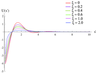
Figure 3: The exact longitudinal range wake for various values of $\xi$.

Fig. 3 shows how the function when evaluated with our numerical technique changes for different values of $\xi$. It can be seen that for values of below about $0.1$ the approximation is very good. For a copper beam pipe with a radius of $1$ cm the scaling length is of order $20$ microns, so $\xi$ is very small in all practical cases at present. However, for possible future collimators with very low conductivity and small radius it might need to be considered. It is also important to check that the simpler formula is valid before using it.

III Longitudinal: Higher order modes

For higher modes, using the same technique of matching the solutions of Maxwell’s equations in the aperture and the pipe, and using the same approximations as for Equation 14 for $m>0$

$$\tilde{E}_{z}^{m}(k)=\frac{2I_{m}}{b^{2m+1}}\frac{1}{\frac{ikb}{m+1}-\frac{\lambda}{k}}$$ (17)

where $I_{m}$ is the charge moment of order $m$: $\int\int\rho(r,\theta)r^{m}\cos(m\theta)\,dr\,d\theta$. Any angular distribution of charges at a particular radius can be described in terms of these moments. Equation 17 can be separated into odd and even parts, taking out a factor of $I_{m}s_{0}/b^{2m+2}$ as before for simplicity

$$f_{even}(K) = -\frac{\frac{2}{\sqrt{K}}}{\Bigl{(}\frac{K}{m+1}-\frac{1}{\sqrt{K}}\Bigr{)}^{2}+\frac{1}{K}}$$

$$f_{odd}(K) = -\frac{2i\Bigl{(}\frac{K}{m+1}-\frac{1}{\sqrt{K}}\Bigr{)}}{\Bigl{(}\frac{K}{m+1}-\frac{1}{\sqrt{K}}\Bigr{)}^{2}+\frac{1}{K}}$$ (18)

Results are shown in Fig. 4. It can be seen that there are quite large differences in behaviour, even though only a few terms in the formula contain an $m$. The value at $s=0$ is given by $U^{m}(0)=-4(m+1)$.

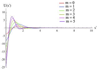
Figure 4: The longitudinal wake for various modes.

The full formula for higher modes, corresponding to Equation 2, is

$$\tilde{E}_{z}^{m}(k)=\frac{4I_{m}}{b^{2m+1}}\frac{1}{\frac{ikb}{m+1}-\Bigr{(}\frac{2k}{\lambda}+\frac{\lambda}{k}\Bigl{)}\Bigr{(}1+\frac{i}{2\lambda b}\Bigl{)}-\frac{im}{kb}}$$ (19)

(Note that Equation 19 is valid only for $m>0$.) This can be separated into odd and even parts as for Equation II.3

$$f_{even}(K) = -8\frac{\xi^{2}+2\xi\sqrt{K}+\frac{4}{\sqrt{K}}}{4\Bigr{[}\xi\sqrt{K}-\frac{1}{K}(\xi+2\sqrt{K})+2\Bigr{(}\frac{K}{m+1}-\xi\frac{m}{K}\Bigl{)}\Bigl{]}^{2}+\Bigr{(}\xi^{2}+\xi 2\sqrt{K}+\frac{4}{\sqrt{K}}\Bigl{)}^{2}}$$

$$f_{odd}(K) = -8i\frac{2\Bigr{[}\xi\sqrt{K}-\frac{1}{K}(\xi+2\sqrt{K})+2\Bigr{(}\frac{K}{m+1}-\xi\frac{m}{K}\Bigl{)}\Bigl{]}}{4\Bigr{[}\xi\sqrt{K}-\frac{1}{K}(\xi+2\sqrt{K})+2\Bigr{(}\frac{K}{m+1}-\xi\frac{m}{K}\Bigl{)}\Bigl{]}^{2}+\Bigr{(}\xi^{2}+\xi 2\sqrt{K}+\frac{4}{\sqrt{K}}\Bigl{)}^{2}}$$ (20)

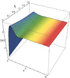
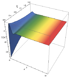
Figure 5: The $m=1$ (top) and $m=5$ (bottom) wake as a function of $s^{\prime}$ and $\xi$.

We show the dependence on $\xi$ in Fig. 5 for $m=1$ and $m=5$. It can be seen that the dependence on $\xi$ increases for higher modes. However even for the $m=5$ mode shown the values of $\xi$ that would correspond to any reasonable beam pipe diameter and conductivity are still so small that the deviation is probably unimportant.

It is frequently stated that the $m=1$ wakefield is related to the $m=0$ wake by a factor ${2\over b^{2}}$. From Fig. 4 it can be seen that the first two angular modes do indeed have the same shape, although higher modes are significantly different. The equality $E^{1}={2\over b^{2}}E^{0}$ is true for Equations 14 and 17, as can be see by making the substitution.

However this is not true for more general formulae, Equations  19 and  II.3, as is shown in Fig. 6. For $\xi=~{}0.5$, which is admittedly large, there is a clear difference between the two curves.

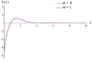
Figure 6: The $m=0$ longitudinal wake, doubled, and the $m=1$ wake for $\xi=0.5$.

IV Transverse wakes

Transverse wake effects are generally of more importance than longitudinal wakes, especially for collimator studies. The transverse wakefield experienced by a particle with transverse position $r$ due to another particle at $r^{\prime}$ can be written as a sum over angular modes

$$\vec{F}_{T}(r,\theta,s)=\sum_{m}r^{m-1}r^{\prime m}(\hat{r}cos(m\theta)-\hat{\theta}sin(m\theta))W^{m}_{T}(s)$$ (21)

where $\theta$ is the angle between the two particles and $s$ is the distance between them. The property 21 applies to the force components and not to the electromagnetic field components(Chao (1993), p.56), and for the transverse wakes the magnetic part has to be included.

The Panofsky-Wenzel theorem

$$\nabla_{T}F={\partial\vec{F}_{T}\over\partial z}$$ (22)

applies term by term giving

$${W^{\prime}}^{m}_{T}(s)=E_{z}^{m}(s).$$ (23)

Thus the transverse wake at any order can be obtained by integrating the longitudinal wake. This is especially convenient for our method as this integral is what is calculated in the inverse transform.

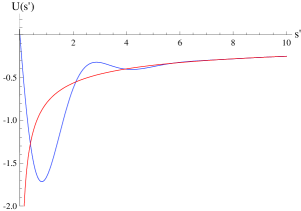
Figure 7: The Transverse wake in the first and second approximation (red and blue curves respectively).

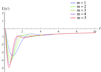
Figure 8: Transverse wakes - various modes with $\xi$=0.

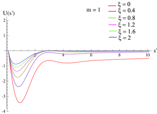
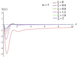
Figure 9: Transverse (top) $m=1$ and (bottom) $m=5$ wakes with $\xi$ variable.

The $m=1$ transverse wake is shown in Fig. 7 for the first and second approximations (equivalent to Chao’s formula and Bane and Sands’ respectively). With our formula we can study the general case. Fig. 8 shows the different transverse modes, for $\xi$=0, and Fig. 9 shows the dependence on $\xi$ for $m=1$ and $m=5$.

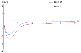
Figure 10: The $m=0$ transverse wake, doubled, and the $m=1$ wake for $\xi=0.5$.

The dominant longitudinal effect is the $m=0$ mode, and the dominant transverse mode is for $m=1$. There is, as Chao makes clear (Chao (1993), p81) no linkage between modes of different orders to be obtained from the Panofsky-Wenzel theorem. However the $m=0$ and $m=1$ longitudinal modes are connected by a simple factor of ${2\over b^{2}}$ as discussed in Section III. In the literature (e.g. Bane and Sands (2006) Equation 3) one finds the expression

$$\tilde{E}_{\perp}^{1}={2\over b^{2}k}\tilde{E}_{||}^{0}$$ (24)

This is exact for resistive wakefields only in the long wavelength approximation. We investigate the validity of this widely-used approximation in the general case. This difference is small, but it is rather larger for the corresponding transverse wakes, as shown in Fig. 10.

V AC Conductivity

In the classical Drude model for the ac conductivity case, in units of normalised wavenumber $K=s_{0}k$, we have

$$\tilde{\sigma}=\frac{\sigma}{1-iK\Gamma}$$ (25)

where we have introduced the dimensionless relaxation factor $\Gamma=c\tau/s_{0}$. For a $1$ cm radius copper tube at room temperature the relaxation time is $\tau=2.7\times 10^{-14}$s or $c\tau=8.1$ $\mu$m giving $\Gamma=0.4$, so we explore $\Gamma$ values in the range $0$ to $5$. In order to calculate the ac resistive wall wakefield the dc conductivity $\sigma$ in Equation 4 is replaced by the general form of the ac conductivity $\tilde{\sigma}$. Hence,

$$\lambda=\frac{b}{s_{0}^{2}}\sqrt{|K|}(1+K^{2}\Gamma^{2})^{-1/4}[i\sqrt{1+t}\pm\sqrt{1-t}]$$ (26)

while

$$\frac{\lambda}{K}=\frac{b}{s_{0}}\frac{1}{\sqrt{|K|}(1+K^{2}\Gamma^{2})^{1/4}}\Bigl{[}[\sqrt{1-t}\pm i\sqrt{1+t}\Bigr{]},$$ (27)

with

$$t=\frac{|K|\Gamma}{\sqrt{1+K^{2}\Gamma^{2}}}.$$ (28)

Following the same procedure employed on Section II we express the inverse Fourier Transform of the m=0 mode of the longitudinal component of the wakefield in terms of the even and odd parts. The simplest of cases given by Equation II.1 becomes,

$$f_{even}(K) = -\frac{\sqrt{1-t}}{l},$$

$$f_{odd}(K) = \frac{i\sqrt{1+t}}{l}$$ (29)

where

$$l=\frac{1}{\sqrt{|K|}(1+K^{2}\Gamma^{2})^{1/4}}.$$ (30)

The results are shown in Fig. 11 for various values of $\Gamma$.

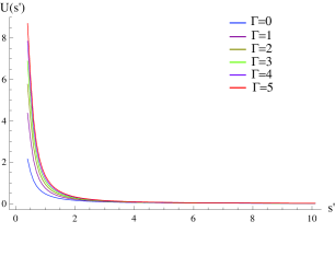
Figure 11: The Long range wake for various values of $\Gamma$.

If we consider the more accurate formula given by Equation 14 our technique gives

$$f_{even}(K) = -\frac{2l\sqrt{1-t}}{\Bigl{(}\frac{K}{2}-l\sqrt{1+t}\Bigr{)}^{2}+l^{2}(1-t)},$$

$$f_{odd}(K) = -\frac{2i\Bigl{(}\frac{K}{2}-l\sqrt{1+t}\Bigr{)}}{\Bigl{(}\frac{K}{2}-l\sqrt{1+t}\Bigr{)}^{2}+l^{2}(1-t)}$$ (31)

For the full version of the dc regime Equation 2 the odd and even parts have counterparts in the ac regime as

$$f_{even}(K)=-8\,l^{2}t(\xi^{2}\sqrt{1-t^{2}}+2\xi lK\sqrt{1-t}$$

$$+4l^{3}K\sqrt{1-t})/d(K)$$

$$f_{odd}(K)=-8i\,l^{2}t\Bigl{[}\xi^{2}t-2\xi l(l-K\sqrt{1+t})$$

$$-4l^{3}K\sqrt{1+t}+2l^{2}K^{2}\Bigr{]}/d(K)$$ (32)

with the denominator given by

$$d(K)=\Bigl{(}\xi^{2}\sqrt{1-t^{2}}+2\xi lK\sqrt{1-t}+4l^{3}K\sqrt{1-t}\Bigr{)}^{2}$$

$$+\Bigl{[}\xi^{2}t-2\xi l(l-K\sqrt{1+t})-4l^{3}K\sqrt{1+t}+2l^{2}K^{2}\Bigr{]}^{2}$$

For $\xi=0$ one can see that Equation V reduces to Bane and Sands’ approximation, Equation V as seen before. Fig. 12 shows the results for various values of $\Gamma$.

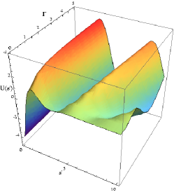
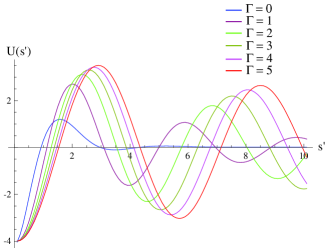
Figure 12: The Longitudinal wake in the second approximation for various $\Gamma$ values.

These wakes show a fairly strong dependence of $\Gamma$ and the effects of AC conductivity may be important in a particular case. However $\xi$ will always be very small so we include it only for completeness and in practice one can probably use $\xi=0$ as a good approximation.

For higher order modes the impedance is given by Equation 19. In the ac regime the odd and even parts are

$$f_{even}(K) = -8\,l^{2}t(\xi^{2}\sqrt{1-t^{2}}+2\xi lK\sqrt{1-t}$$

$$+4l^{3}K\sqrt{1-t})/d(K)$$

$$f_{odd}(K) = -8i\,l^{2}t\Bigl{[}\xi^{2}t-2\xi l(l-K\sqrt{1+t})$$

$$-4l^{3}K\sqrt{1+t}+4l^{2}\Bigl{(}\frac{K^{2}}{m+1}-m\xi\Bigr{)}\Bigr{]}/d(K)$$

with the denominator given by

$$d(K) = \Bigl{(}\xi^{2}\sqrt{1-t^{2}}+2\xi lK\sqrt{1-t}+4l^{3}K\sqrt{1-t}\Bigr{)}^{2}$$

$$+\Bigl{[}\xi^{2}t-2\xi l(l-K\sqrt{1+t})-4l^{3}K\sqrt{1+t}$$

$$+4l^{2}\Bigl{(}\frac{K^{2}}{m+1}-m\xi\Bigr{)}K^{2}\Bigr{]}^{2}$$

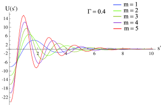
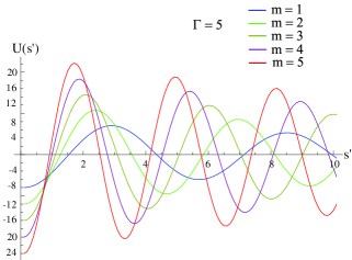
Figure 13: The longitudinal wake for various modes ($m>0$) for $\Gamma=0.4$ (top) and $\Gamma=5$ (bottom).

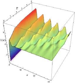
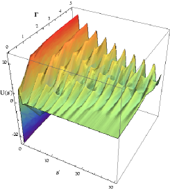
Figure 14: The m=1 (top) and m=5 (bottom) longitudinal wake as a function of $\Gamma$.

In Fig. 13 we show the different modes dependance for two particular values of $\Gamma$, $0.4$ and $5.0$ and $\xi=0$.

The $\Gamma$ dependence of two modes, mode $m=1$ and $m=5$ is shown in Fig. 14 also for $\xi=0$. The equivalent transverse wake is shown in Fig. 15. It is clear that for all modes, increasing $\Gamma$ increases the size of the wake effect, both longitudinal and transverse over the same distance. For the higher modes the effect is stronger.

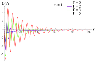
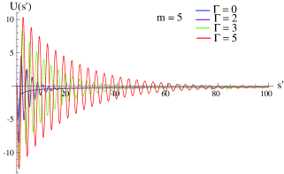
Figure 15: The m=1 (top) and m=5 (bottom) transversal wake for various values of $\Gamma$, all for $\xi$=0.

VI Implementation

The integrals used to generate the plots in this paper were performed using Mathematica Mat . Tables with $6\times 1001\times 21$ elements were written to file, covering the ranges $0\leq\Gamma\leq 5$, $0\leq s^{\prime}\leq 100$ and $0\leq\xi\leq 2$ respectively. A separate table was used for each mode, and tables were written separately for longitudinal and transverse wakes.

For ease of use we have defined a small object collimatortable written in C++ but portable between Merlin, Placet, and hopefully other simulation codes. When created by a call to the constructor collimatortable(filename, Gamma, xi) it will read the full 3 dimensional table from filename and construct a one dimensional table, using parabolic interpolation between the 9 closest points, for $s^{\prime}$ at this value of $\Gamma$ and of $\xi$, both of which default to zero. It does this because when tracking particles through a collimator the values of $s$ (or $s^{\prime}$) are different for each pair of particles (or slices), whereas the values of $\Gamma$ and $\xi$ are the same, as they depend on the properties of the collimator, not the bunch. Then the one dimensional table can be used by the member function collimatortable::interpolate(sprime) to find the value for any value of $s^{\prime}$ in the range.

These data and program files are obtainable from the authors our .

VI.1 MERLIN

The MERLIN program Mer contains a general wake formalism which has been extended Bungau and Barlow for high order modes (though only for axially symmetric apertures) and it is easy to incorporate these wakefields. A class ResistivePotentials which inherits from SpoilerWakePotentials calculates $\Gamma$ and $\xi$ from the dimensions and properties given and uses collimatortable to read the files; functions Wtrans(z,m) and Wlong(z,m) use the interpolate function to get the wake experienced by the particles.

For efficiency, the bunch is divided longitudinally into a number of slices $N_{s}$ (typically $100$) and each wake function is called only $N_{s}(N_{s}-1)/2$ times.

VI.2 PLACET

The PLACET program Latina and et al. (2006) contains only the lowest order $m=1$ transverse mode, though it does include the effect of rectangular apertures using as an Ansatz the Yokoya factors $y_{eff}=0.822y_{1}+0.411y_{2}$, where $y_{1}$ and $y_{2}$ are the displacements of the leading and trailing particle. $y_{eff}$ is then used in the formula for circular apertures.

In the current implementation a complicated system switches between different formulae depending on the sizes of the pipe and bunch. The integral resulting from the analytic transform of Equation 14 is calculated numerically. We replace these with a single call to the interpolate function. $100$ lines of code in the original are replaced by $21$ lines in the new version. The wake function is called for each slice for each macroparticle, $~{}N_{s}N_{p}/2$ times.

VII Examples

VII.1 Simple collimator

As a numerical example we consider a $1$ m long collimator made of Titanium, with conductivity $\sigma=2.33\times 10^{6}\,(\Omega m)^{-1}$. The radius is $1.4$ mm and the relaxation time is $2.7\times 10^{-14}\$s. This gives $s_{0}=0.165\,\mu$m, $\Gamma=0.49$ and $\xi=0.00014$.

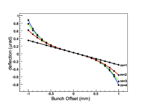
Figure 16: Merlin prediction for the deflection as a function of offset.

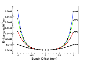
Figure 17: Merlin prediction for emittance as a function of offset.

This collimator and the beam bunch properties are those of the recent tests at SLAC End Station A Woods , with $\beta_{x}=128.2$ m, $\beta_{y}=11.9$ m, $\epsilon_{x}=5.49\times 10^{-9}$ m, $\epsilon_{y}=3.44\times 10^{-10}$ m, initial beam energy $p=28.5$ GeV and bunch length $\sigma_{z}=0.3$ mm, with the sole difference of $\epsilon_{x}=\epsilon_{y}=3.44\times 10^{-10}$ m when using Merlin. The bunch of $N_{p}=10^{10}$ particles was modelled by $50000$ macroparticles in both simulations.

We show the predictions of Merlin (PLACET) for the mean kick of the bunch in Fig. 16 (Fig. 18) and for the increased geometric emittance in Fig. 17 (Fig. 19), respectively. The total emittance increase leading to the loss of luminosity at the IP caused by wakefields is due in part to jitter amplification and in part to the increased size of the bunch itself Zimmermann et al. (1996). This latter effect is what we show. If one considers a bunch as a series of slices it is clear that different slices receive different angular kicks, the first slice receiving no kick at all, and this difference between slices increases the angular size of the bunch as a whole.

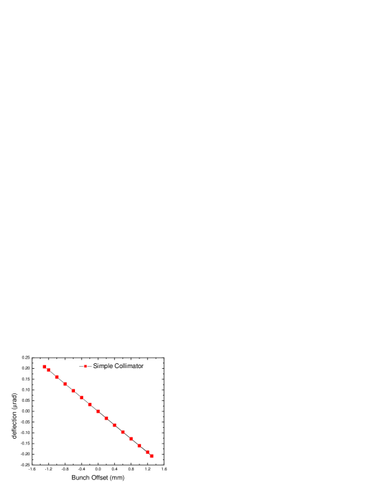
Figure 18: PLACET prediction for the deflection as a function of offset.

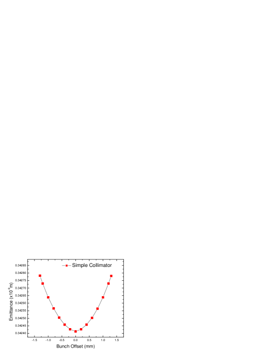
Figure 19: PLACET prediction for emittance as a function of offset.

The deflection of Figs. 16 and 18 compounded with transverse jitter, may also contribute to the loss of luminosity by an amount that depends on the betatron phases at the collimator and at the IP. In previous analyses, such as Tenenbaum , Toader and et al. (2008) it was assumed that the incoherent intrinsic increase of emittance is $0.4$ times coherent term produced by jitter. Here we show that it can be calculated explicitly.

The results from Merlin and PLACET agree surprisingly well, given that one uses the Yokoya terms and the other does not. The overall shift in the emittance of Figs. 17 and 19 is due to the different random bunches and using only $50000$ macro particles. Merlin results show that higher modes become important (only) for offset $\geq b/2$.

VII.2 Extreme collimator

We consider a $1$ m long collimator made of graphite, with conductivity $\sigma=7.14\times 10^{4}(\Omega m)^{-1}$ and very narrow pipe of radius $0.125$ mm. This gives $s_{0}=0.105\,\mu$m, $\Gamma=2.85$ and $\xi=0.007$. For comparison purposes we consider a beam bunch of the same properties as for the previous collimator, but with the emittance ten times smaller, while the displacements of the beam from the central axis are between $0$ and $0.115$ mm.

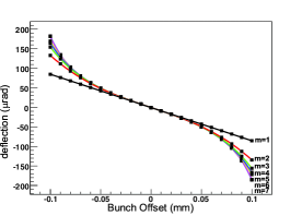
Figure 20: Merlin prediction for the deflection as a function of offset.

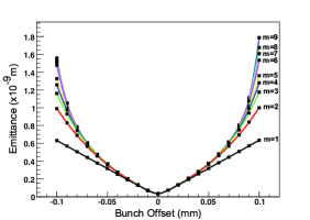
Figure 21: Merlin prediction for emittance as a function of offset.

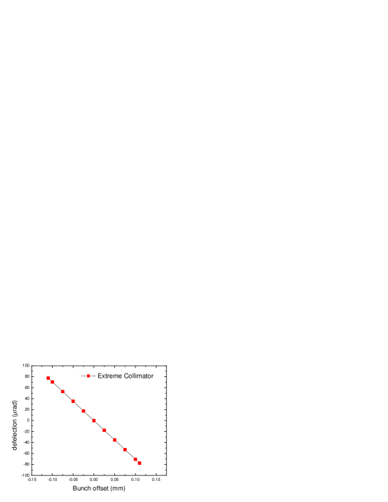
Figure 22: PLACET prediction for the deflection as a function of offset.

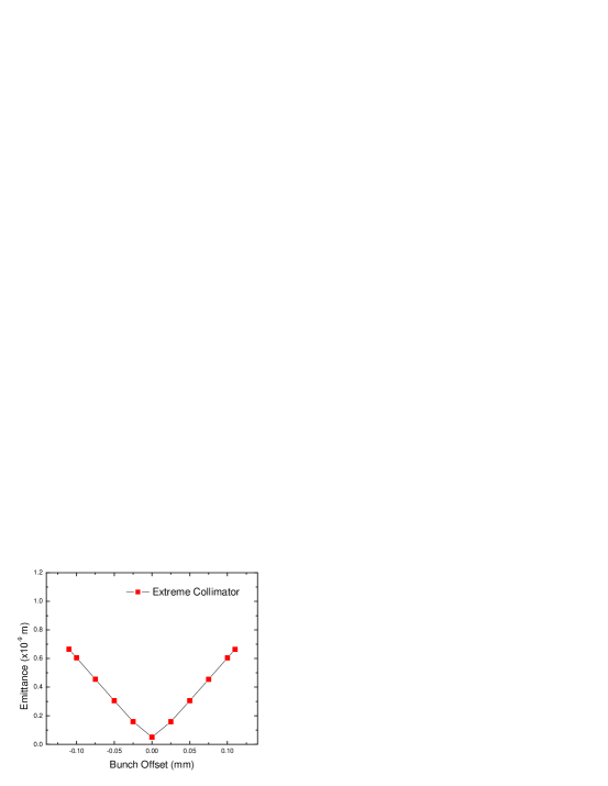
Figure 23: PLACET prediction for emittance as a function of offset.

Again, the agreement is good (Figs. 20 - 23). Merlin shows that higher modes become significant sooner than they do for the previous case. Also it can be seen that more modes are needed for convergence when the bunch displacement is large compared to pipe radius.

VIII Conclusions

Longitudinal and transverse resistive wakes can be calculated in simulations programs with a technique applicable for any general particle separation using pretabulated numerical Fourier Transforms and implemented in a way which is computationally efficient. Higher order angular modes can easily be included, and so can be AC conductivity effects. We have shown that this can be used by the Merlin, PLACET programs and other codes can be added in due curse. Results are given for two types of collimator, and show that the effects are as expected. This can be used in simulations of full beamline lattice for accelerators such as CLIC and the LHC.

References

- Chao (1993) A. M. Chao, Physics of Collective Beam Instabilities in High Energy Accelerators John Wiley and Sons (New York) (1993).
- Latina and et al. (2006) A. Latina and et al., Recent improvements in PLACET, ICAP2006 p. 188 (2006).
- Bane (1991) K. L. F. Bane, The Short Range Resistive Wall Wakefields, Preprint SLAC/AP-87 (1991).
- Bane and Sands (1995) K. L. F. Bane and M. Sands, The Short Range Resistive Wall Wakefields, Preprint SLAC-PUB-95-7074 (1995).
- Gluckstern et al. (1993) R. L. Gluckstern, J. van Zeits, and B. Zotter, Phys. Rev. E47, 656 (1993).
- Yokoya (1993) K. Yokoya, Part. Accel. 41, 221 (1993).
- Lutman et al. (2008) A. Lutman, R. Vescovo, and P. Craievich, Phys. Rev. ST Accel. Beams 11, 074401 (2008).
- Bane and Sands (2006) K. L. F. Bane and M. Sands, Wakefields of Sub-Picosecond Electron Bunches, Preprint SLAC-PUB-11829 (2006).
- (9) eprint Wolfram Research Inc., Mathematica, Version 6, Champaign IL (2007).
- (10) eprint http://www.hep.man.ac.uk/adina.
- (11) eprint The Merlin program, http://www.desy.de.
- (12) A. Bungau and R. Barlow, eprint Simulation of High Order Short Range Wake Fields for Particle Tracking Codes. In preparation.
- (13) M. Woods, eprint Test beam studies at SLAC End Station A for the International Linear Collider, MOPP007, EPAC06.
- Zimmermann et al. (1996) F. Zimmermann, K. L. F. Bane, and C. K. Ng, Collimator Wake in the SLC Final Focus, SLAC-PUB-7137 (1996).
- (15) P. Tenenbaum, eprint Collimator Wakefield Calculations for ILC-TRC Report, LCC-NOTE-101, SLAC-TN-03-38.
- Toader and et al. (2008) A. M. Toader and et al., Effect of collimator wakefields in the BDS of the ILC, WEPP167, EPAC08 (2008).