Brownian motion under annihilation dynamics

Abstract

The behavior of a heavy tagged intruder immersed in a bath of particles evolving under ballistic annihilation dynamics is investigated. The Fokker-Planck equation for this system is derived and the peculiarities of the corresponding diffusive behavior are worked out. In the long time limit, the intruder velocity distribution function approaches a Gaussian form, but with a different temperature from its bath counterpart. As a consequence of the continuous decay of particles in the bath, the mean squared displacement increases exponentially in the collision per particle time scale. Analytical results are finally successfully tested against Monte Carlo numerical simulations.

I Introduction

In recent years, there has been some interest for systems where particles annihilate ballistically bnklr ; bek ; ks ; t02 ; ptd02 ; cdt04 ; cdt04s ; llf06 . In these studies, the model considered consists of an ensemble of hard particles which evolve freely until a binary encounter, which leads either to the annihilation of the colliding partners with probability $p$, or to an elastic collision with probability $1-p$. For this probabilistic annihilation model, there are no collisional invariants, and numerical simulations have shown that for a broad class of initial conditions, the system reaches an homogeneous state in which all the time dependence of the one particle distribution function is encoded in the density and temperature (defined as the second velocity moment of the distribution function) t02 ; ptd02 . This is the so-called “Homogeneous Decay State”. Such a behavior resembles the one of granular fluids (see bte05 and references therein) where, if the system is stable, it evolves into an homogeneous cooling state, in which all the time dependence is borne by the granular temperature (in this case the density is conserved) gs95 . For the annihilation model, the hydrodynamic equations have been derived using the Chapmann-Enskog method chapman60 by the usual assumption of the existence of a “normal solution”, whose space and time dependence occurs only through the hydrodynamic fields cdt04 . Recently, the hydrodynamic equations linearized around the homogeneous decay state have been derived relaxing such an assumption gmsbt08 . Nevertheless, it must be assumed that there is scale separation, i.e that the spectrum of the linearized Boltzmann collision operator is such that the eigenvalues associated to the hydrodynamic excitations are separated from the faster “kinetic eigenvalues”. Although this property is valid for elastic collisions mclennan , it has not been proven for the probabilistic ballistic annihilation model in general, but only for Maxwell molecules ernst and for $p$ smaller than a given threshold gmsbt08 .

The objective in this paper is to study the simplest transport process in this system in which we can rigorously prove that there is scale separation. We will consider a tagged particle in a fluid in the homogeneous decay state, but collisions between the tagged particle and the particles of the fluid will be always elastic. The equation for the tagged particle is the Boltzmann-Lorentz equation resibois ; mclennan which depends on the one particle distribution function of the bath. In the limit of asymptotically large relative mass for the tagged particle, this equation reduces to a Fokker-Planck equation which depends on the time-dependent density and temperature of the bath. Due to the structure of this equation, we can prove that there is scale separation and that, in the long-time limit, the velocity distribution function of the tagged particle approaches a Gaussian distribution but with a temperature that differs from that of the bath. A similar breakdown of equipartition has been reported for a heavy particle in a granular bath mp99 ; bds99 ; brgd99 ; dbl02th ; bt02 , a problem that can be mapped onto an elastic situation sd06 , at variance with the situation under scrutiny here. We also study the diffusion of the heavy particle and identify the diffusion coefficient as a Green-Kubo formula in terms of the velocity autocorrelation function. Finally, we perform Monte Carlo numerical simulations in order to test our theoretical results.

II Fokker-Planck equation

We consider a tagged particle of mass $m$ and diameter $\sigma$ immersed in a low-density gas. This gas is composed of hard spheres or disks of mass $m_{g}$ and diameter $\sigma_{g}$ which move ballistically until one particle meets another one; such binary encounters lead to the annihilation of the colliding partners with probability $p$ or to an elastic collision with probability $1-p$ bnklr ; bek ; ks ; t02 ; ptd02 ; llf06 . Collisions between the particles of the gas and the tagged particle are always elastic.

II.1 From Boltzmann-Lorentz to Fokker-Planck

The evolution equation for the probability density $F(\mathbf{r},\mathbf{v},t)$ of the tagged particle is the Boltzmann-Lorentz equation resibois ; mclennan

$$\left(\frac{\partial}{\partial t}+\mathbf{v}\cdot\nabla\right)F(\mathbf{r},\mathbf{v},t)=J[\mathbf{r},\mathbf{v},t|F,f],$$ (1)

where the collision operator is given by

$$J[\mathbf{r},\mathbf{v},t|F,f] = \sigma_{0}^{d-1}\int\!\!d\mathbf{v}_{1}\!\!\int\!\!d\bm{\hat{\sigma}}\Theta(\mathbf{g}\cdot\bm{\hat{\sigma}})(\mathbf{g}\cdot\bm{\hat{\sigma}})\left\{F(\mathbf{r},\mathbf{v}^{*},t)f(\mathbf{r},\mathbf{v}^{*}_{1},t)\right.$$ (2)

$$- \left.F(\mathbf{r},\mathbf{v},t)f(\mathbf{r},\mathbf{v}_{1},t)\right\}.$$

Here $f(\mathbf{r},\mathbf{v},t)$ is the distribution function of the particles in the gas, $d$ is the space dimension, $\mathbf{g}=\mathbf{v}-\mathbf{v}_{1}$ is the relative velocity, $\Theta$ is the Heaviside step function, $\bm{\hat{\sigma}}$ is a unit vector pointing from the centre of the gas particle to the centre of the tagged particle at contact, and $\sigma_{0}=\frac{\sigma+\sigma_{g}}{2}$. The precollisional velocities $\mathbf{v}^{*}$ and $\mathbf{v}_{1}^{*}$ are given by

$$\mathbf{v}^{*}=\mathbf{v}-\frac{2\Delta}{1+\Delta}(\mathbf{g}\cdot\bm{\hat{\sigma}})\bm{\hat{\sigma}},$$ (3)

$$\mathbf{v}_{1}^{*}=\mathbf{v}_{1}+\frac{2}{1+\Delta}(\mathbf{g}\cdot\bm{\hat{\sigma}})\bm{\hat{\sigma}},$$ (4)

with $\Delta=m_{g}/m$ the (gas/tagged particle) mass ratio.

We shall consider that the gas is in the homogeneous decay state, so its distribution function has the scaling form ptd02

$$f_{H}(\mathbf{v}_{1},t)=\frac{n_{g}(t)}{v_{g}^{d}(t)}\chi_{H}({c}_{1}),\qquad\mathbf{c}_{1}=\frac{\mathbf{v}_{1}}{v_{g}(t)},$$ (5)

where $n_{g}(t)$ is the number density of the gas, $v_{g}(t)=\left(\frac{2T_{g}(t)}{m_{g}}\right)^{1/2}$ is the thermal velocity of the particles in the gas and $\chi_{H}$ is an isotropic function depending only on the modulus $c=|\mathbf{c}|$ of the rescaled velocity. It can be seen that the homogeneous density and temperature obey the following equations cdt04

$$\frac{\partial n_{g}(t)}{\partial t} = -p\nu_{g}(t)\zeta_{n}n_{g}(t),$$ (6)

$$\frac{\partial T_{g}(t)}{\partial t} = -p\nu_{g}(t)\zeta_{T}T_{g}(t),$$ (7)

where we have introduced the collision frequency of the corresponding hard sphere fluid in equilibrium (with same temperature and density)

$$\nu_{g}(t)=\frac{n_{g}(t)\,T^{1/2}_{g}(t)\,\sigma_{g}^{d-1}}{m^{1/2}}\frac{8\pi^{\frac{d-1}{2}}}{(d+2)\Gamma(d/2)}.$$ (8)

Here the dimensionless decay rates $\zeta_{n}$ and $\zeta_{T}$ are functionals of the distribution function and are approximately known in the first Sonine approximation t02 ; cdt04s , see Appendix A. Equations (6) and (7) can be integrated to obtain the following power laws for the decay of the density and temperature

$$n_{g}(t) = n_{g}(0)\left[1+\nu_{g}(0)p(\zeta_{n}+\zeta_{T}/2)t\right]^{-\frac{2\zeta_{n}}{2\zeta_{n}+\zeta_{T}}},$$ (9)

$$T_{g}(t) = T_{g}(0)\left[1+\nu_{g}(0)p(\zeta_{n}+\zeta_{T}/2)t\right]^{-\frac{2\zeta_{T}}{2\zeta_{n}+\zeta_{T}}}.$$ (10)

As a consequence, we get $n_{g}T_{g}^{1/2}\propto t^{-1}$, a simplified form of a scaling relation common to all ballistically controlled processes TH95 .

We next study the evolution equation for the tagged particle in the limit of large relative mass for the tagged particle. In the limit $\Delta\ll 1$, it is possible to expand the collision operator $J[\mathbf{r},\mathbf{v},t|F,f]$ in powers of $\Delta$. In Appendix B it is shown that the leading order is

$$J[\mathbf{r},\mathbf{v},t|F,f]\simeq\frac{\partial}{\partial\mathbf{v}}\cdot[\mathbf{A}(\mathbf{v})F(\mathbf{r},\mathbf{v},t)]+\frac{1}{2}\frac{\partial}{\partial\mathbf{v}}\frac{\partial}{\partial\mathbf{v}}:[N(\mathbf{v})F(\mathbf{r},\mathbf{v},t)],$$ (11)

where

$$\mathbf{A}(\mathbf{v},t)=\gamma(t)\mathbf{v},\qquad N(\mathbf{v},t)=2\bar{\gamma}(t)I,$$ (12)

and $I$ is the second order unit tensor. The definitions of $\gamma$ and $\bar{\gamma}$ are respectively

$$\gamma(t) = \gamma_{e}[n_{g}(t),T_{g}(t)]a(p),$$ (13)

$$\bar{\gamma}(t) = \gamma_{e}[n_{g}(t),T_{g}(t)]a(p)b(p)\frac{T_{g}(t)}{m},$$ (14)

The friction coefficient $\gamma_{e}(t)$ is the same as for elastic bodies, and appears here as a function of the time-dependent density $n_{g}(t)$ and temperature $T_{g}(t)$

$$\gamma_{e}[n_{g}(t),T_{g}(t)]=\frac{4\pi^{\frac{d-1}{2}}}{d\Gamma(d/2)}\Delta^{1/2}n_{g}(t)\left(\frac{2T_{g}(t)}{m}\right)^{1/2}\sigma_{0}^{d-1},$$ (15)

with $a(p)$ and $b(p)$ functionals of the distribution function of the bath which depend only on the parameter $p$

$$a(p) = \frac{\Gamma(d/2)}{\Gamma((d+1)/2)}\int\!\!d\mathbf{c}_{1}\chi_{H}(c_{1})c_{1},$$ (16)

$$b(p) = \frac{2}{d+1}\frac{\int\!\!d\mathbf{c}_{1}\chi_{H}(c_{1})c_{1}^{3}}{\int\!\!d\mathbf{c}_{1}\chi_{H}(c_{1})c_{1}}.$$ (17)

In Appendix B, it is shown that the two terms on the right hand side of equation (11) are both of order $n_{g}v_{g}\sigma_{0}^{d-1}\Delta$, while the other contributions in the Kramers-Moyal expansion are at least of order $n_{g}v_{g}\sigma_{0}^{d-1}\Delta^{3/2}$. In the same Appendix, the expressions for $a(p)$ and $b(p)$ are evaluated to first order in a Sonine expansion.

Taking into account the approximate expression for the collision operator, Eq. (11), it is possible to write the Boltzmann-Lorentz equation as a Fokker-Planck equation for asymptotically small $\Delta$

$$\left[\frac{\partial}{\partial t}+\mathbf{v}\cdot\nabla\right]F(\mathbf{r},\mathbf{v},t)=\gamma_{e}(t)a(p)\frac{\partial}{\partial\mathbf{v}}\cdot\left[\mathbf{v}+b(p)\frac{T_{g}(t)}{m}\frac{\partial}{\partial\mathbf{v}}\right]F(\mathbf{r},\mathbf{v},t).$$ (18)

As in the inelastic case, the Einstein relation is violated due to the fact that the distribution function of the bath is not Maxwellian bds99 ; dg01 ; blp04 ; g04 , which in turn implies that $b(p)\neq 1$. On the other hand, if we suppose that the velocity of the tagged particle obeys a Markov process and write the corresponding Fokker-Planck equation, in terms of the jump moments, $\lim_{\Delta t\to 0}\langle\Delta v\rangle/\Delta t$ and $\lim_{\Delta t\to 0}\langle\Delta v^{2}\rangle/\Delta t$, we obtain exactly Eq. (18). Here $\langle\dots\rangle$ means average over different noise (bath) realizations.

II.2 Coarse grained fields and relevant scales

We now focus on the study of the hydrodynamic fields of the tagged particle with the aid of the Fokker-Planck equation, Eq. (18). We define the mean velocity and the temperature of the Brownian particle as

$$\mathbf{u}(t) = \int\!\!d\mathbf{r}\!\!\int\!\!d\mathbf{v}\mathbf{v}F(\mathbf{r},\mathbf{v},t),$$ (19)

$$\frac{d}{2}T(t) = \int\!\!d\mathbf{r}\!\!\int\!\!d\mathbf{v}\frac{1}{2}m(\mathbf{v}-\mathbf{u})^{2}F(\mathbf{r},\mathbf{v},t).$$ (20)

Taking moments in the Fokker-Planck equation, we obtain (see Appendix C)

$$\frac{\partial\mathbf{u}(t)}{\partial t} = -\gamma_{e}(t)a(p)\mathbf{u}(t),$$ (21)

$$\frac{\partial T(t)}{\partial t} = -2\gamma_{e}(t)a(p)[T(t)-b(p)T_{g}(t)].$$ (22)

As the function $\gamma_{e}$ is a known functional of the gas density $n_{g}$ and temperature $T_{g}$, equations (21) and (22) can be integrated, which yields

$$\mathbf{u}(t)=\mathbf{u}(0)\left[1+\nu_{g}(0)p(\zeta_{n}+\zeta_{T}/2)t\right]^{-\frac{a(p)\zeta_{T}}{(2\zeta_{n}+\zeta_{T})\epsilon}},$$ (23)

and

$$T(t) = \frac{b(p)T_{g}(0)}{1-\epsilon}\left[1+\nu_{g}(0)p(\zeta_{n}+\zeta_{T}/2)t\right]^{-\frac{2\zeta_{T}}{2\zeta_{n}+\zeta_{T}}}$$ (24)

$$+ \left[T(0)-\frac{b(p)T_{g}(0)}{1-\epsilon}\right]\left[1+\nu_{g}(0)p(\zeta_{n}+\zeta_{T}/2)t\right]^{-\frac{2\zeta_{T}}{\epsilon(2\zeta_{n}+\zeta_{T})}}.$$

In the above equation, we have introduced the dimensionless coefficient $\epsilon$

$$\epsilon=\frac{p\zeta_{T}\nu_{g}(t)}{2a(p)\gamma_{e}(t)}=\frac{\sqrt{2}d\zeta_{T}}{2(d+2)a(p)}\left(\frac{\sigma_{g}}{\sigma_{0}}\right)^{d-1}\frac{p}{\Delta},$$ (25)

that is not necessarily a small quantity.

As can be seen in Eq. (24), the behavior of the temperature depends strongly on the value of $\epsilon$. If $\epsilon<1$ the first term of equation (24) dominates in the long time limit and the temperature of the tagged particle asymptotically decays with the same power as the temperature of the gas (see equation (10)). As a consequence of (24) we have

$$\lim_{t\to\infty}\frac{T(t)}{T_{g}(t)}=\frac{b(p)}{1-\epsilon},\qquad\epsilon<1.$$ (26)

On the other hand, if $\epsilon>1$ the second term of equation (24) dominates in the long time limit and the temperature decays slower than the gas temperature. One can understand this behavior as follows; the parameter $\epsilon$ is essentially the quotient between the cooling rate of the gas and the relaxation rate of the tagged particle’s temperature. If the former is smaller than the latter, the tagged particle’s temperature is eventually slaved by $T_{g}$ due to the second term of the Eq. (22). In the reversed case, the tagged particle’s temperature evolves independently in the long time limit with a cooling rate slower than that of the gas. It should be emphasized here that in the expansion made in the previous section, we implicitly assumed that $T/T_{g}$ remains finite, because the coefficients $\mathbf{A}$ and $N$ were expanded in powers of $\Delta^{1/2}\frac{T}{T_{g}}$ (see Appendix B). Hence, the Fokker-Planck equation for $\epsilon>1$ is restricted to a time window in which $\frac{T}{T_{g}}$ is small enough. In the following, we will only consider the case in which the Fokker-Planck equation is valid for all times, i.e. the double limit

$$\Delta\to 0,\qquad p\to 0,\qquad\epsilon<1,\qquad\epsilon\propto\left(\frac{\sigma_{g}}{\sigma_{0}}\right)^{d-1}\frac{p}{\Delta},$$ (27)

where the requirement of small $p$ stems from $\Delta\ll 1$ and $\epsilon$ bounded from above. Hence, in order to be consistent with this limit, we can substitute in the Fokker-Planck equation, Eq. (18), the values of the coefficients, $a(p)$ and $b(p)$ by their elastic limits

$$\lim_{p\to 0}a(p)=1,\qquad\lim_{p\to 0}b(p)=1,$$ (28)

so that

$$\left[\frac{\partial}{\partial t}+\mathbf{v}\cdot\nabla\right]F(\mathbf{r},\mathbf{v},t)=\gamma_{e}(t)\frac{\partial}{\partial\mathbf{v}}\cdot\left[\mathbf{v}+\frac{T_{g}(t)}{m}\frac{\partial}{\partial\mathbf{v}}\right]F(\mathbf{r},\mathbf{v},t).$$ (29)

This equation is formally identical to the one obtained for an elastic gas resibois , except for the fact that the density and temperature of the gas depend on time. This is a consequence of the elastic limit to which we are restricted. In general, the coefficients $a(p)$ and $b(p)$, Eqs. (16) and (17), differ from unity due to the non Maxwellian character of the distribution function of the bath, and Einstein relation is violated.

In order to analyze this equation, it is convenient to introduce the dimensionless time scale, $t^{*}$, proportional to the number of collisions of the tagged particle

$$t^{*}=(1-\epsilon_{0})\int_{0}^{t}dt^{\prime}\gamma_{e}(t^{\prime}),$$ (30)

where $\epsilon_{0}$ is defined by substituting $\zeta_{T}(p)/a(p)$ in (25) by its $p\to 0$ limit:

$$\epsilon_{0}=\frac{\sqrt{2}}{16}\left(\frac{\sigma_{g}}{\sigma_{0}}\right)^{d-1}\frac{p}{\Delta}.$$ (31)

The dimensionless time scale $t^{*}$ is related to the real time $t$ by

$$t^{*}=\frac{\gamma_{e}2(1-\epsilon_{0})}{\nu_{g}}\frac{1}{p(2\zeta_{n}+\zeta_{T})}\log[1+\nu_{g}(0)p(\zeta_{n}+\zeta_{T}/2)t].$$ (32)

In this time scale, the evolution of the mean velocity and temperature of the tagged particle are particularly simple

$$\mathbf{u}(t^{*})=\mathbf{u}(0)e^{-\frac{t^{*}}{1-\epsilon_{0}}},$$ (33)

and

$$\frac{T(t^{*})}{T_{g}(t^{*})}=\frac{T(0)}{T_{g}(0)}e^{-2t^{*}}+\frac{1}{1-\epsilon_{0}}(1-e^{-2t^{*}}).$$ (34)

Such predictions will be compared against numerical simulations in section IV. Let us also introduce the scaled distribution

$$F(\mathbf{r},\mathbf{v},t)=\frac{1}{v_{\epsilon}^{d}(t)}F^{*}(\mathbf{r},\mathbf{v}^{*},t^{*}),\qquad\mathbf{v}^{*}=\frac{\mathbf{v}}{v_{\epsilon}(t)},$$ (35)

where

$$v_{\epsilon}(t)=\left(\frac{1}{1-\epsilon_{0}}\right)^{1/2}\left(\frac{2T_{g}(t)}{m}\right)^{1/2}.$$ (36)

The function $v_{\epsilon}(t)$ is introduced because with these definitions we have

$$v_{\epsilon}(t)\to\left[\frac{2T(t)}{m}\right]^{1/2},$$ (37)

in the long time limit. In these variables the Fokker-Planck equation (29) reduces to

$$\left(\frac{\partial}{\partial t^{*}}+\ell_{0}(t^{*})\mathbf{v}^{*}\cdot\nabla\right)F^{*}(\mathbf{r},\mathbf{v}^{*},t^{*})=\Lambda_{FP}(v^{*})F^{*}(\mathbf{r},\mathbf{v}^{*},t^{*}),$$ (38)

where we have introduced the standard homogeneous Fokker-Planck operator

$$\Lambda_{FP}(v^{*})=\frac{\partial}{\partial\mathbf{v}^{*}}\cdot\left(\mathbf{v}^{*}+\frac{1}{2}\frac{\partial}{\partial\mathbf{v}^{*}}\right),$$ (39)

and the function proportional to the mean free path

$$\ell_{0}(t^{*})=\frac{v_{\epsilon}(t)}{(1-\epsilon_{0})\gamma_{e}(t)}=\frac{d\Gamma(d/2)}{(1-\epsilon_{0})^{3/2}4\pi^{\frac{d-1}{2}}}\Delta^{-1/2}\left(\frac{\sigma_{g}}{\sigma_{0}}\right)^{d-1}[n_{g}(t^{*})\sigma_{g}^{d-1}]^{-1}.$$ (40)

Taking into account the definition of $\epsilon$, Eq. (25), we can write explicitly $\ell_{0}$ as a function of the $t^{*}$ variable as

$$\ell_{0}(t^{*})=\ell_{0}(0)e^{\epsilon^{*}t^{*}},\qquad\epsilon^{*}=\frac{2\zeta_{n}\epsilon_{0}}{\zeta_{T}(1-\epsilon_{0})}.$$ (41)

To sum up, we have obtained the evolution equation for the distribution function of a tagged particle in a bath of particles which annihilate, in the limit where the tagged particle is much heavier than the particles of the bath. There are some points in common with the elastic case, but also some important differences. The homogeneous operator, whose spectral properties are well-known resibois ; mclennan , is exactly the same, but the flux term is weighted by a function depending on time and that diverges in the long time limit. This will have important consequences in the study of diffusion as we will see in the following section. Moreover, the equation is not valid for all values of the probability $p$ of annihilation in the bath and masses of the tagged particle but, as already mentioned, is limited to the double limit of Eq. (27), in which $\epsilon_{0}<1$.

III Long-time limit solution of the Fokker-Planck equation

In this section we investigate the long time behavior of the solution of the Fokker-Planck equation, Eq. (38), starting with an arbitrary initial condition. The objective is to study if the tagged particle reaches some scaling state in the long time limit and also to analyze how the particle diffuses.

III.1 Evolution towards a scaling form

As the Fokker-Planck equation is linear, it is convenient to work in the Fourier space. The Fourier component of the tagged particle distribution function is defined as

$$F_{\mathbf{k}}(\mathbf{v}^{*},t^{*})=\int\!\!d\mathbf{r}e^{-i\mathbf{k}\cdot\mathbf{r}}F^{*}(\mathbf{r},\mathbf{v}^{*},t^{*}),$$ (42)

so that Eq. (38) yields $F_{\mathbf{k}}(\mathbf{v}^{*},t^{*})$

$$\frac{\partial}{\partial t^{*}}F_{\mathbf{k}}(\mathbf{v}^{*},t^{*})=[\Lambda_{FP}(v^{*})-i\ell_{0}(t^{*})\mathbf{k}\cdot\mathbf{v}^{*}]F_{\mathbf{k}}(\mathbf{v}^{*},t^{*}).$$ (43)

The spectrum of the operator $\Lambda_{FP}(v^{*})-i\ell_{0}(t^{*})\mathbf{k}\cdot\mathbf{v}^{*}$ is known resibois ; mclennan . The eigenvalues are

$$\lambda_{\mathbf{n}}(\mathbf{k},t)=-\frac{1}{2}[k\ell_{0}(t)]^{2}-\sum_{j=1}^{d}n_{j},$$ (44)

where we have introduced the vector label $\mathbf{n}=(n_{1},\dots,n_{d})$, with possible coordinate values $n_{i}=0,1,2,\dots\infty$. Hence, for any initial condition, all the $\mathbf{k}$-Fourier components decay and only the $\mathbf{k}=\mathbf{0}$ remains. Moreover, as the eigenfunction associated to the vanishing eigenvalue is the Maxwellian distribution resibois ; mclennan

$$\chi_{M}(\mathbf{v}^{*})=\frac{1}{\pi^{d/2}}e^{-v^{*2}},$$ (45)

we obtain

$$F(\mathbf{r},\mathbf{v},t)\to\frac{1}{v_{\epsilon}^{d}(t)}\chi_{M}{(v^{*})},$$ (46)

in the long time limit.

As a consequence, the tagged particle distribution function approaches a scaling form similar to (5) for the gas, but with a different temperature (see (26)). In this regime the cooling rates of the bath and of the tagged particle are the same and the temperatures are proportional. The situation is similar to that of an elastic particle in a bath of inelastic grains bds99 ; brgd99 . Nevertheless, there is an important difference: in the inelastic case it has been proved that there exists an exact mapping with an elastic system. On the other hand, in our problem such a mapping fails due to the flux term which explicitly depends on time.

III.2 Characteristics of diffusive motion

Our objective is to study the evolution equation for the density of tagged particles, $n(\mathbf{r},t)=\int d\mathbf{v}F(\mathbf{r},\mathbf{v},t)$ in a “macroscopic” scale, i.e. in a long time and length scale compared to the microscopic ones. The microscopic time scale is defined by the slowest kinetic modes of $\Lambda_{FP}$, i.e. the modes with a single non vanishing component, labeled by $n_{i}=\delta_{ij}$ for a given value of $j$ in $[1,d]$. The microscopic length scale is defined by the mean free path of the tagged particle which is proportional to $\ell_{0}(t^{*})$. The starting point will be the Fokker-Planck equation for $F_{\mathbf{k}}$, Eq. (43). As the generator of the dynamics, the operator $\Lambda_{FP}(v^{*})-i\ell_{0}(t^{*})\mathbf{k}\cdot\mathbf{v}^{*}$, does not commute with its time derivative, it is not possible to write the general solution of equation (43) in terms of the initial condition in a simple way. Nevertheless, it is shown in Appendix D that in the hydrodynamic limit, i.e. $k\ell_{0}(t^{*})\ll 1$ for all the time evolution and $t^{*}\gg 1$, a closed equation for the Fourier component of the density, $n_{\mathbf{k}}=\int d\mathbf{v}^{*}F_{\mathbf{k}}(\mathbf{v}^{*},t^{*})$, is obtained

$$\frac{\partial n_{\mathbf{k}}(t^{*})}{\partial t^{*}}=-D_{0}[k\ell_{0}(t^{*})]^{2}n_{\mathbf{k}}(t^{*}),$$ (47)

where the diffusion coefficient is

$$D_{0}=\frac{1}{2(1+\epsilon^{*})}.$$ (48)

This asymptotic behavior can be evaluated, taking advantage of the scale separation (i.e. the mode with $\mathbf{n}=\mathbf{0}$ is isolated from the other modes). From equation (47) we can derive the evolution equation for the density

$$\frac{\partial n(\mathbf{r},t^{*})}{\partial t^{*}}=D_{0}\ell_{0}^{2}(t^{*})\nabla^{2}n(\mathbf{r},t^{*}).$$ (49)

This is the equation we were looking for and it is only valid in the “macroscopic” time and length scale. If we transform this equation to real time with the aid of formula (30) we obtain

$$\frac{\partial n(\mathbf{r},t)}{\partial t}=D(t)\nabla^{2}n(\mathbf{r},t),\qquad D(t)=\frac{\zeta_{T}}{(1-\epsilon_{0})[\zeta_{T}+(2\zeta_{n}-\zeta_{T})\epsilon_{0}]}D_{e}(t),$$ (50)

where $D_{e}(t)=2v_{g}^{2}(t)/\gamma_{e}(t)$ is the same as the diffusion coefficient for elastic collisions except that it appears here as a function of the time-dependent gas temperature and density. As can be seen, for our system the diffusion coefficient $D(t)$ is far from being a trivial generalization of the elastic diffusion coefficient.

Now let us focus on the predictions of our diffusion equation. To this end, we introduce the mean square displacement

$$\langle r^{2}(t^{*})\rangle=\int\!d\mathbf{r}\,r^{2}n(\mathbf{r},t^{*}).$$ (51)

If we consider an infinite system, we obtain from equation (49)

$$\frac{\partial}{\partial t^{*}}\langle r^{2}(t^{*})\rangle=2dD_{0}\ell_{0}(t^{*})^{2},$$ (52)

that will only be valid in the long time limit. It is straightforward to integrate equation (52), taking into account the explicit formula for $\ell_{0}(t^{*})$, Eq. (41). This gives

$$\langle r^{2}(t^{*})\rangle=dD_{0}\ell_{0}^{2}(0)\frac{e^{2\varepsilon^{*}t^{*}}-1}{\varepsilon^{*}},$$ (53)

or in real time

$$\langle r^{2}(t)\rangle=\frac{dD_{0}\ell_{0}^{2}(0)}{\epsilon^{*}}\left\{\left[1+\nu_{g}(0)p(\zeta_{n}+\zeta_{T}/2)t\right]^{\frac{4\zeta_{n}}{2\zeta_{n}+\zeta_{T}}}-1\right\}.$$ (54)

As can be seen in Eq. (53), the diffusive behavior is completely different from its elastic or even inelastic counterparts, where it was found that the mean square displacement is proportional to the number of collision per particle bds99 ; brgd99 . The fact that the bath is loosing particles significantly affects this dynamics, and the mean square displacement increases exponentially in the collision per particle scale. As we will see in the following section, simulation results agree well with our theoretical prediction. Roughly speaking, the exponent $4\zeta_{n}/(2\zeta_{n}+\zeta_{T})$ is close to $8d/(4d+1)$ (approximately 1.77 in two dimensions, and 1.84 in three dimensions).

III.3 Diffusive behavior : an alternative derivation

In the remainder of this section, we show that, under plausible hypothesis, it is possible to re-derive “à la Einstein” the formula for the mean square displacement, Eq. (53). This derivation has the merit of leading to a Green-Kubo like expression for the diffusion coefficient. We start by writing the mean-squared displacement as

$$\langle r^{2}(t)\rangle=\int_{0}^{t}dt^{\prime}\int_{0}^{t}dt^{\prime\prime}\langle\mathbf{V}(t^{\prime})\cdot\mathbf{V}(t^{\prime\prime})\rangle.$$ (55)

Here, the position and the velocity of the tagged particle, $\mathbf{r}(t)$ and $\mathbf{V}(t)$, are considered as a stochastic process and $\langle\dots\rangle$ denotes an ensemble average over different trajectories. Let us change the variables from $t\to t^{*}$ and let us also introduce the scaled velocity

$$\mathbf{w}(t^{*})\equiv\frac{\mathbf{V}}{v_{\epsilon}(t)},$$ (56)

where $v_{\epsilon}(t)$ is defined in (36). With these definitions we have

$$\langle r^{2}(t^{*})\rangle = \frac{1}{(1-\epsilon_{0})^{2}}\int_{0}^{t^{*}}ds_{1}\gamma^{-1}_{e}(s_{1})\int_{0}^{t^{*}}ds_{2}\gamma^{-1}_{e}(s_{2})\langle\mathbf{V}(s_{1})\cdot\mathbf{V}(s_{2})\rangle$$ (57)

$$= \ell_{0}^{2}(0)\int_{0}^{t^{*}}ds_{1}\int_{0}^{t^{*}}ds_{2}e^{\epsilon^{*}(s_{1}+s_{2})}\langle\mathbf{w}(s_{1})\cdot\mathbf{w}(s_{2})\rangle,$$

where we have used the definitions of $t^{*}$ and $\ell_{0}(0)$, Eq. (30) and Eq. (41). Now, if we assume that the tagged particle is in the scaled regime, i.e. the temperature is $T_{g}(t^{*})/(1-\epsilon_{0})$ and that the correlation function $\langle\mathbf{w}(s_{1})\cdot\mathbf{w}(s_{2})\rangle$ is a function of $s_{1}-s_{2}$, by integrating in the new variables $S=(s_{1}+s_{2})/2$ and $s=s_{1}-s_{2}$, the following relation is obtained

$$\frac{\langle r^{2}(t^{*})\rangle}{e^{2\epsilon^{*}t^{*}}}\frac{\epsilon^{*}}{d\ell_{0}^{2}(0)}\to\frac{1}{d}\int_{0}^{t^{*}}ds\langle\mathbf{w}(s)\cdot\mathbf{w}(0)\rangle e^{-\epsilon^{*}s},$$ (58)

in the long time limit. This formula is the generalization of the Einstein formula for the diffusion coefficient of a heavy particle in a fluid in the homogeneous decay state. It relates the asymptotic behavior of the mean-square displacement with the time integral of the autocorrelation function of the velocity weighted by the exponential $e^{-\epsilon^{*}s}$. So far we have considered the Fokker-Planck equation as the equation for the one-time probability distribution function. If we assume that the velocity of the tagged particle is a Markov process, then the Fokker-Planck equation is also the equation for the conditional probability and we can evaluate easily the correlation function $\langle\mathbf{w}(s_{1})\cdot\mathbf{w}(s_{2})\rangle$. Taking into account Eqs. (33) and (36), we have

$$\langle\mathbf{w}(s_{1})\cdot\mathbf{w}(s_{2})\rangle=\frac{d}{2}e^{-|s_{1}-s_{2}|}.$$ (59)

By substituting this formula into Eq. (58) we re-derive Eq. (53) with the same diffusion coefficient $D_{0}$, that can be written in the Green-Kubo form

$$D_{0}=\frac{1}{d}\int_{0}^{\infty}ds\langle\mathbf{w}(s)\cdot\mathbf{w}(0)\rangle e^{-\epsilon^{*}s}.$$ (60)

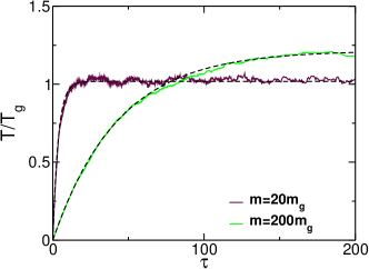
Figure 1: (Color online) Evolution of the temperature ratio as a function of the number of collisions per particle $\tau$ for a system with $p=0.01$ and two values of the tagged particle’s mass, $m=20m_{g}$ ($\Delta=1/20$) and $m=200m_{g}$ ($\Delta=1/200$). The dashed line is the theoretical prediction given by Eq. (34).

IV Direct Simulation Monte Carlo results

The objective of this section is to put to the test the main results of the previous sections by means of the direct simulation Monte Carlo method (DSMC). More precisely, we will analyze the temperature and mean velocity evolution, together with the tagged particle diffusion. We have performed DSMC simulations of a system of $N_{g}$ hard disks of mass $m_{g}$ and diameter $\sigma_{g}$ which annihilate with probability $p$ or collide elastically with probability $1-p$ everytime two particles meet. Bird’s algorithm bird has been used. The parameters in all the simulations were $m_{g}=1$, $\sigma_{g}=1$, $N_{g}(0)=10^{5}$ and $T_{g}(0)=1$. We have considered only one tagged particle in each simulation, that collides elastically with the surrounding bath. The diameter of this particle has been set to unity ($\sigma=1$) and we have varied the value of its mass $m$. The values of the probability of annihilation $p$ of the particles in the bath have been $p=0.1$ and $p=0.01$, and the results have been averaged over $2\cdot 10^{4}$ and $4\cdot 10^{3}$ trajectories respectively. For a given value of $p$, we have performed a series of simulations for different values of the mass of the tagged particle. Taking due account of the constraint $\epsilon_{0}<1$, the value of the tagged particle’s mass must be smaller than $10^{2}$ for $p=0.1$ and $10^{3}$ for $p=0.01$.

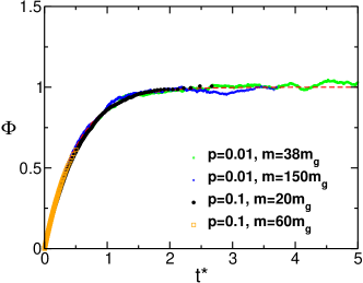
Figure 2: (Color online) Scaling function $\Phi$ defined in the main text as a function of reduced time $t^{*}$ for different systems with $p=0.1$ and $p=0.01$ and different values of the tagged particle’s mass. The dashed line is the theoretical prediction of Eq. (62).

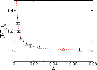
Figure 3: (Color online) Stationary values of the temperatures ratio for a system with $p=0.01$ and different values of the tagged particle’s mass $\Delta=m_{g}/m$. Symbols are for the Monte Carlo data and the dashed line shows the long time limit of Eq. (34).

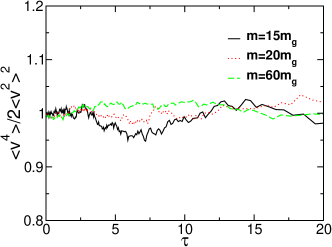
Figure 4: (Color online) Reduced fourth moment of the tagged particle velocity as a function of the dimensionless time $\tau$ for $p=0.1$ and different values of the tagged particle’s mass.

Figure 1 shows the evolution of the ratio $T/T_{g}$ for a system with $p=0.01$ and for two values of the tagged particle’s mass, that is, $m=20m_{g}$ and $m=200m_{g}$, as a function of the number of collisions per particle, $\tau$, defined as

$$\tau=\frac{1}{2}\int_{0}^{t}dt^{\prime}\nu_{g}(t^{\prime})=\frac{1}{2(1-\epsilon_{0})}\frac{\nu_{g}}{\gamma_{e}}t^{*}.$$ (61)

The initial value of temperature of the tagged particle is $T(0)=0$ for all the trajectories, since at $t=0$, the intruder has a prescribed velocity. As we can see, in this scale, the evolution to the stationary value of the ratio of the temperatures is slower as we increase the mass of the tagged particle. This implies that there are values of the tagged particle’s mass for which the ratio of the temperatures will not reach its stationary value in the time of the simulation (for instance, the number of particles in the bath for $\tau=200$ is $N_{g}\simeq 1800$, which hinders correct statistical sampling). The theoretical prediction in this time scale (dashed line) is obtained directly from Eq. (34), taking into account Eq. (61). The agreement between theory and simulations is good.

Similar simulations were performed with different values of the tagged particle mass ($m$ ranging from 15 to 100 for $p=0.1$ and from 15 to 900 for $p=10^{-2}$). Since $T_{g}(0)=0$, Eq. (34) predicts

$$\Phi\,\equiv\,(1-\epsilon_{0})\frac{T}{T_{g}}\,=\,1-e^{-2t^{*}}.$$ (62)

As can be observed in Fig. 2, all simulation data for $\Phi$ collapse onto a single curve. The time scale $t^{*}$ can be calculated from the scale $\tau$ defined in (61). In the same vein, we can obtain the stationary value of the temperature ratio, which is plotted as a function of $\Delta=m_{g}/m$ in Fig. 3 ; this validates our theoretical analysis.

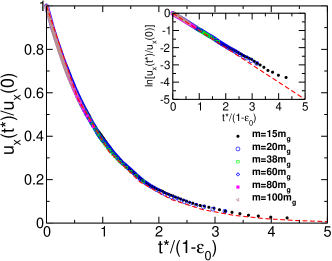
Figure 5: (Color online) Mean velocity of the tagged particle as a function of $t^{*}/(1-\epsilon_{0})$ for a system with $p=0.1$ and several values of the tagged particle’s mass. The dashed line is the theoretical prediction given by Eq. (33). Inset: Mean velocity of the tagged particle as a function of $t^{*}/(1-\epsilon_{0})$ for a system with $p=0.1$ on a logarithmic scale.

In order to probe –at least partially– the Gaussian nature of the time dependent tagged particle velocity statistics, we have measured the reduced fourth moment $4\langle v^{4}\rangle/(d(d+2)\langle v^{2}\rangle^{2})$. As can be seen in Fig. 4, where we have plotted the results for $p=0.1$ and several values of $\Delta$ as a function of the number of collisions per particle, $\tau$, the value of this quantity is in agreement with the Gaussian prediction (that is unity) within the statistical uncertainties.

Consider next the mean velocity of the tagged particle, $\mathbf{u}(t^{*})$. In order to study the decay of this quantity, we have performed a set of simulations starting with a component of the velocity field in the $x$ direction when it is immersed in a bath in the homogeneous decay state, $u_{x}(0)$. In Fig. 5, we plot $u_{x}(t^{*})/u_{x}(0)$ as a function of $t^{*}/(1-\epsilon_{0})$ for $p=0.1$ and several values of $m$. In this time scale, the data for all values of $m$ collapse due to Eq. (33). In the inset, the same quantity is plotted on a logarithmic scale. If the theoretical prediction in Eq. (33) is verified, the above plot must lead to a straight line with slope $\zeta_{\mathbf{u}}=1$ (dashed line), where $\zeta_{\mathbf{u}}$ is the decay rate of the mean velocity. On the other hand, $\zeta_{\mathbf{u}}$ can be fitted on the logarithmic plot of the inset. Reporting the corresponding measures in Fig. 6 against the mass ratio, it appears that the theoretical prediction $\zeta_{\mathbf{u}}=1$ is approached as $\Delta\to 0$, as expected.

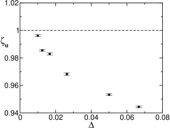
Figure 6: Decay rate of the mean velocity as a function of $\Delta$ for a system with $p=0.1$. The symbols are from DSMC simulations an the dashed line is the theoretical prediction.

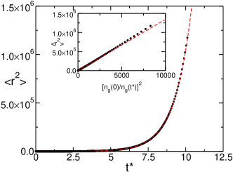
Figure 7: (Color online) Mean squared displacement for a system with $p=0.01$ and $m=60m_{g}$ as a function of $t^{*}$. The dashed line is the theoretical prediction, Eq. (53). Inset : same quantity as a function of $n_{g}(0)^{2}/n_{g}(t^{*})^{2}$. The dashed line is the theoretical prediction of Eq. (63) where $B$ follows from (65).

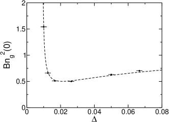
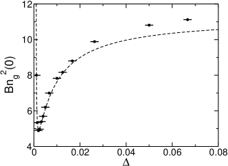
Figure 8: Values of $Bn_{g}^{2}(0)$ as a function of $\Delta$ for systems with $p=0.1$ (left) and $p=0.01$ (right). The dashed line is for the prediction of Eq. (65).

Finally, the accuracy of the prediction for the diffusion equation has also been tested by measuring in DSMC simulations the mean square displacement of the tagged particle. In contrast to the granular case phenomenology and as a consequence of the continuous decay of particles in the bath, the mean squared displacement increases exponentially in the $t^{*}$ scale, see Eq. (53). In Fig. 7 we have plotted the time evolution of $\langle r^{2}\rangle$ in the scale $t^{*}$ for a system with $p=0.01$ and $m=60m_{g}$. The dashed line is the theoretical prediction given by Eq. (53), and shows good agreement with numerical data. The same quantity, written in terms of the bath density, reads

$$\langle r^{2}(t^{*})\rangle = dD_{0}\ell_{0}^{2}(0)\frac{e^{2\epsilon^{*}t^{*}}-1}{\epsilon^{*}}$$ (63)

$$= B\left[\frac{n_{g}(0)^{2}}{n_{g}(t^{*})^{2}}-1\right],$$

where we have defined

$$B=\frac{dD_{0}\ell_{0}^{2}(0)}{\varepsilon^{*}},$$ (64)

and we have taken into account that $n_{g}(t^{*})=n_{g}(0)e^{-\epsilon^{*}t^{*}}$. It then appears that the mean squared displacement increases linearly with $n_{g}(0)^{2}/n_{g}(t^{*})^{2}$. This is full agreement with the simulation results, see the inset of Fig 7. Such a plot allows us to extract by linear fitting the coefficient $B$, which can then be compared against the prediction of Eq. (64), which explicitly reads

$$B=-\frac{16\sqrt{2}d^{2}\pi^{1-d}\sigma_{g}^{2(1-d)}\Gamma\left(\frac{d}{2}\right)^{2}}{n_{g}^{2}(0)p(-16+\sqrt{2}\frac{p}{\Delta})(16+\sqrt{2}(4d-1)\frac{p}{\Delta})},$$ (65)

where we have taken into account that $\sigma_{0}=\sigma_{g}$. Such a comparison is worked out in Figure 8 and fully corroborates the theoretical analysis, with again an improved agreement when $\Delta$ decreases.

It would be also interesting to confirm our theoretical predictions with Molecular Dynamics simulations. In the low density limit, it is expected to get similar results. In fact, some simulations were performed finding qualitatively the same behavior but with much more statistical inaccuracies.

V Conclusions

In this paper, the diffusive behavior of a tagged intruder immersed in a gas of particles undergoing ballistic annihilation (i.e. which annihilate with probability $p$ or scatter elastically otherwise), has been analyzed. The collisions between the tagged particle and the surrounding gas are elastic. Some similarities are found between our system and the elastic or inelastic case resibois ; bds99 , but, on the other hand, important differences arise as a consequence of the continuous decay of particle number in the system.

We start from the Boltzmann-Lorentz equation for the distribution function of the tagged particle, which is valid, in principle, for arbitrary mass of the tagged particle. In the limit of a very massive tagged particle, a Fokker-Planck equation for the distribution function is derived by means of a systematic expansion in the mass ratio $\Delta$. Our approach holds in the limit $\Delta\ll 1$, but we additionally have the more stringent condition that the parameter introduced in Eq. (25), $\epsilon\propto\frac{p}{\Delta}$, must be smaller than unity. Analysis of the Fokker-Planck equation leads to predictions for the temperature ratio, the decay rate of the mean velocity of the tagged particle and the diffusion coefficient. As in the inelastic case bds99 , the theory predicts that the ratio between the temperatures of the tagged particle and the gas is constant in the long time limit as a consequence of equilibrating cooling rates. When represented in the appropriate time scale, which is proportional to the number of collisions experienced by the tagged particle, temperature ratios collapse for all values of $\Delta$ and $p$ considered. Likewise, the mean intruder velocity (averaged over bath realizations) decays exponentially. The dynamics of the distribution function of the tagged particle is governed by a Fokker-Planck operator which spectral properties are known. More specifically, as the eigenvalues of this operator are non-positive, the distribution of the tagged particle approaches a Gaussian in the long-time limit and admits a scaling form similar to the one for the distribution function for the particles in the gas but with a different temperature. At variance with the situation of an elastic intruder in a bath of inelastic particles sd06 , there is apparently no mapping between our problem and a well chosen elastic system. A unique vanishing eigenvalue is responsible for the slow diffusive behavior of the tagged particle density. The corresponding diffusion equation has been derived in the hydrodynamic limit, by means of a projector decomposition, which yields an explicit expression for the diffusion coefficient. From a different point of view, the expression for the mean squared displacement has also been derived “à la Einstein”. Following this route, the diffusion coefficient is expressed as a Green-Kubo formula in terms of a weighted time integral of the tagged particle velocity correlation function. This provides a more physical perspective on the results derived from the projector method. As already mentioned, the mean squared displacement for this system does not increase linearly in the collision per particle time scale, as is the case in the elastic and inelastic cases. This different behavior is due to the time dependent bath density. In the elastic case, both the temperature and the density do not depend on time. In an inelastic system bds99 ; brgd99 , the time dependence goes through the temperature and could be absorbed in the collision per particle time scale, which turns out to be impossible in our system where the mean free path $\ell(t^{*})$ is an increasing function of time.

Finally, our analytical results have been tested by numerical simulations, and a very good agreement has been reported for all the range of parameters considered. As expected, the agreement is all the better as $\Delta$ is smaller. In summary, the work reported here provides an example of the accuracy of hydrodynamics to describe a system in which there are no conserved quantities in binary encounters (no collisional invariants).

Appendix A Some useful approximations

For the sake of completeness, we provide here the approximate expressions for the density and temperature decay rates, that are relevant for explicit computation of several of the quantities discussed in the main text. They have been obtained from a truncated Sonine expansion (Sonine polynomials being particular types of Laguerre polynomials, particularly convenient for kinetic theory calculus) t02 ; ptd02 ; cdt04 .

$$\zeta_{n} = \frac{d+2}{4}\left(1-a_{2}\frac{1}{16}\right),$$ (66)

$$\zeta_{T} = \frac{d+2}{8d}\left(1+a_{2}\frac{8d+11}{16}\right),$$ (67)

where

$$a_{2}=\frac{8(3-2\sqrt{2})p}{(4d+6-\sqrt{2})p+8\sqrt{2}(d-1)(1-p)}.$$ (68)

Appendix B From the Boltzmann-Lorentz equation to the Fokker-Planck equation

In this Appendix we expand the collision operator, Eq. (2), in series of $\Delta$. We start by multiplying the collision operator by a generic function $H(\mathbf{v})$ and integrate in velocity space

$$\int\!\!d\mathbf{v}H(\mathbf{v})J[\mathbf{r},\mathbf{v},t|F,f]$$

$$=\sigma_{0}^{d-1}\int\!\!d\mathbf{v}\!\!\int\!\!d\mathbf{v}_{1}H(\mathbf{v})\!\!\int\!\!d\hat{\bm{\sigma}}\Theta(\mathbf{g}\cdot\hat{\bm{\sigma}})(\mathbf{g}\cdot\hat{\bm{\sigma}})[F(\mathbf{v}^{*})f(\mathbf{v}_{1}^{*})-F(\mathbf{v})f(\mathbf{v}_{1})].$$

The above expression can be written

$$\int\!\!d\mathbf{v}H(\mathbf{v})J[\mathbf{r},\mathbf{v},t|F,f]$$

$$=\sigma_{0}^{d-1}\int\!\!d\mathbf{v}\!\!\int\!\!d\mathbf{v}_{1}F(\mathbf{v})f(\mathbf{v}_{1})\!\!\int\!\!d\hat{\bm{\sigma}}\Theta(\mathbf{g}\cdot\hat{\bm{\sigma}})(\mathbf{g}\cdot\hat{\bm{\sigma}})[H(\mathbf{v}-\delta\mathbf{v})-H(\mathbf{v})],$$

where we have introduced

$$\delta\mathbf{v}=\frac{2\Delta}{1+\Delta}(\mathbf{g}\cdot\hat{\bm{\sigma}})\hat{\bm{\sigma}},$$ (71)

which is the increment of the tagged particle velocity due to collisions with a particle of the bath (it should be remembered that $\mathbf{g}=\mathbf{v}-\mathbf{v}_{1}$). Equation (B) essentially tells us how the function $H$ varies due to collisions. If we admit that $\Delta$ is small enough, we can expand $H(\mathbf{v}-\delta\mathbf{v})$ around $\mathbf{v}$ in powers of $\delta\mathbf{v}$, keeping only the lower orders

$$H(\mathbf{v}-\delta\mathbf{v})\simeq H(\mathbf{v})-\left[\frac{\partial H(\mathbf{v})}{\partial\mathbf{v}}\right]\cdot\delta\mathbf{v}+\frac{1}{2}\left[\frac{\partial}{\partial\mathbf{v}}\frac{\partial}{\partial\mathbf{v}}H(\mathbf{v})\right]:\delta\mathbf{v}\delta\mathbf{v}.$$ (72)

If we introduce expansion (72) in equation (B) we obtain

$$\int\!\!d\mathbf{v}H(\mathbf{v})J[\mathbf{r},\mathbf{v},t|F,f]$$

$$\simeq\int\!\!d\mathbf{v}H(\mathbf{v})\left\{\frac{\partial}{\partial\mathbf{v}}\cdot[\mathbf{A}(\mathbf{v})F(\mathbf{v})]+\frac{1}{2}\frac{\partial}{\partial\mathbf{v}}\frac{\partial}{\partial\mathbf{v}}:[N(\mathbf{v})F(\mathbf{v})]\right\},$$ (73)

where we have introduced

$$\mathbf{A}(\mathbf{v})=\frac{2\Delta\pi^{\frac{d-1}{2}}\sigma_{0}^{d-1}}{(1+\Delta)\Gamma\left(\frac{d+3}{2}\right)}\int\!\!d\mathbf{v}_{1}f(\mathbf{v}_{1})g\mathbf{g},$$ (74)

$$N(\mathbf{v})=\left[\frac{2\Delta}{1+\Delta}\right]\frac{\pi^{\frac{d-1}{2}}\sigma_{0}^{d-1}}{\Gamma\left(\frac{d+5}{2}\right)}\int\!\!d\mathbf{v}_{1}f(\mathbf{v}_{1})\left[\frac{d+3}{2d}g^{3}\mathbf{I}+\frac{3}{2}g\left(\mathbf{g}\mathbf{g}-\frac{1}{d}g^{3}\mathbf{I}\right)\right].$$ (75)

In the last expression $\mathbf{I}$ is the unit tensor. As $H(\mathbf{v})$ is a generic function of $\mathbf{v}$, we can compare equations (B) and (B), and we obtain that the collision operator can be written as

$$J[\mathbf{r},\mathbf{v},t|F,f]\simeq\frac{\partial}{\partial\mathbf{v}}\cdot[\mathbf{A}(\mathbf{v})F(\mathbf{v})]+\frac{1}{2}\frac{\partial}{\partial\mathbf{v}}\frac{\partial}{\partial\mathbf{v}}:[N(\mathbf{v})F(\mathbf{v})].$$ (76)

We next specify $\mathbf{A}$ and $N$ within the scaling form provided by the homogeneous decay state of the bath. This will lead us to identify the remaining $\Delta$ dependence in these coefficients and to simplify the functional dependence in the tagged particle velocity. To this end, we introduce the dimensionless velocities

$$\mathbf{c}=\frac{\mathbf{v}}{v_{0}(t)},\qquad\mathbf{c}_{1}=\frac{\mathbf{v}_{1}}{v_{g}(t)},$$ (77)

where $v_{g}(t)=\left(\frac{2T_{g}(t)}{m_{g}}\right)^{1/2}$ and $v_{0}(t)=\left(\frac{2T(t)}{m}\right)^{1/2}$, with $T(t)$ the temperature of the tagged particle and $T_{g}(t)$ the temperature of the suspending gas. The relative velocity $\mathbf{g}=\mathbf{v}-\mathbf{v}_{1}$ can be written as

$$\mathbf{g}=v_{g}(t)\left[\frac{T(t)}{T_{g}(t)}\right]^{1/2}\Delta^{1/2}\mathbf{c}-v_{g}(t)\mathbf{c}_{1}.$$ (78)

A formal expansion in $(T/T_{g})\Delta$ leads to

$$\mathbf{A}(\mathbf{v},t)=\gamma(t)\mathbf{v},\qquad N(\mathbf{v},t)=2\bar{\gamma}(t)\mathbf{I}.$$ (79)

The definitions of $\gamma$ and $\bar{\gamma}$ are respectively

$$\gamma(t) = \gamma_{e}[n_{g}(t),T_{g}(t)]a(p),$$ (80)

$$\bar{\gamma}(t) = \gamma_{e}[n_{g}(t),T_{g}(t)]a(p)b(p)\frac{T_{g}(t)}{m},$$ (81)

where $\gamma_{e}(t)$ is the same friction coefficient as for an elastic system at the corresponding density and temperature

$$\gamma_{e}[n_{g}(t),T_{g}(t)]=\frac{4\pi^{\frac{d-1}{2}}}{d\Gamma(d/2)}\Delta^{1/2}n_{g}(t)\left(\frac{2T_{g}(t)}{m}\right)^{1/2}\sigma_{0}^{d-1},$$ (82)

and $a$, $b$ are functionals of the distribution function of the bath which depend only on the parameter $p$

$$a(p) = \frac{\Gamma(d/2)}{\Gamma((d+1)/2)}\int\!\!d\mathbf{c}_{1}\chi_{H}(c_{1})c_{1},$$ (83)

$$b(p) = \frac{2}{d+1}\frac{\int\!\!d\mathbf{c}_{1}\chi_{H}(c_{1})c_{1}^{3}}{\int\!\!d\mathbf{c}_{1}\chi_{H}(c_{1})c_{1}}.$$ (84)

These coefficients have been evaluated in the first Sonine approximation and depend very weakly on $p$

$$a(p) = \frac{8-a_{2}(p)}{8},$$ (85)

$$b(p) = \frac{8+3a_{2}(p)}{8-a_{2}(p)},$$ (86)

where $a_{2}$, defined in (68), is the gas velocity distribution kurtosis (a Gaussian ansatz would amount to setting $a_{2}=0$). By dimensional analysis and taking into account the explicit formulas for $\mathbf{A}$ and $N$, equation (79), we can see that the two terms we have considered in the expansion of the collision operator, Eq. (76), are of order $n_{g}v_{g}\sigma_{0}^{d-1}\Delta$, while the other terms in the Kramers-Moyal expansion are at least of order $n_{g}v_{g}\sigma_{0}^{d-1}\Delta^{3/2}$. Hence, we can conclude that the leading order contribution in $\Delta$ of the collision operator is actually the one written in (76).

Appendix C Equations for the velocity and temperature of the tagged particle

In this Appendix we derive the equations for the mean velocity and temperature of the tagged particle. Taking moments in the Fokker-Planck equation, Eq. (18), we obtain for the velocity

$$\frac{\partial\mathbf{u}(t)}{\partial t}=\int\!\!d\mathbf{r}\!\!\int\!\!d\mathbf{v}\mathbf{v}\left\{-(\mathbf{v}\cdot\nabla)+\gamma_{e}(t)a(p)\frac{\partial}{\partial\mathbf{v}}\cdot\mathbf{v}\right.$$

$$\left.+a(p)b(p)\frac{T_{g}}{m}\gamma_{e}(t)\frac{\partial^{2}}{\partial\mathbf{v}^{2}}\right\}F(\mathbf{r},\mathbf{v},t).$$ (87)

By integration we have

$$\frac{\partial\mathbf{u}(t)}{\partial t} = \int\!\!d\mathbf{r}\!\!\int\!\!d\mathbf{v}\mathbf{v}\gamma_{e}(t)a(p)\frac{\partial}{\partial\mathbf{v}}\cdot(\mathbf{v}F(\mathbf{r},\mathbf{v},t))$$ (88)

$$= -\int\!\!d\mathbf{r}\!\!\int\!\!d\mathbf{v}\gamma_{e}(t)a(p)\mathbf{v}F(\mathbf{r},\mathbf{v},t)$$ (89)

$$= -\gamma_{e}(t)a(p)\mathbf{u}(t).$$ (90)

Consequently, the equation for the mean velocity is

$$\frac{\partial\mathbf{u}(t)}{\partial t}=-\gamma_{e}(t)a(p)\mathbf{u}(t).$$ (91)

Taking into account the definition of temperature,

$$\frac{d}{2}T(t) = \int\!\!d\mathbf{r}\!\!\int\!\!d\mathbf{v}\frac{1}{2}m[\mathbf{v}-\mathbf{u}(t)]^{2}F(\mathbf{r},\mathbf{v},t)$$ (92)

$$= \int\!\!d\mathbf{r}\!\!\int\!\!d\mathbf{v}\frac{1}{2}m[v^{2}-u^{2}(t)]F(\mathbf{r},\mathbf{v},t).$$

we can write

$$\frac{d}{2}\frac{\partial}{\partial t}T(t)=\frac{m}{2}\left[\frac{\partial}{\partial t}\int\!\!d\mathbf{r}\!\!\int\!\!d\mathbf{v}{v}^{2}F(\mathbf{r},\mathbf{v},t)-2\mathbf{u}(t)\cdot\frac{\partial\mathbf{u}(t)}{\partial t}\right].$$ (93)

In order to evaluate the first term on the right hand side, we make use of the Fokker-Planck equation:

$$\frac{\partial}{\partial t}\int\!\!d\mathbf{r}\!\!\int\!\!d\mathbf{v}{v}^{2}F(\mathbf{r},\mathbf{v},t)=-2\gamma_{e}(t)a(p)\int\!\!d\mathbf{r}\!\!\int\!\!d\mathbf{v}{v}^{2}F(\mathbf{r},\mathbf{v},t)+\frac{2d}{m}T_{g}\gamma_{e}(t)a(p)b(p).$$ (94)

Taking this formula and the equation for the velocity into account, we obtain

$$\frac{d}{2}\frac{\partial T(t)}{\partial t}=-d\gamma_{e}(t)a(p)[T(t)-b(p)T_{g}(t)].$$ (95)

Appendix D The diffusion equation

In this Appendix we derive the diffusion equation for the tagged particle’s density. The starting point is the Fokker-Planck equation (43)

$$\frac{\partial}{\partial t^{*}}F_{\mathbf{k}}(\mathbf{v}^{*},t^{*})=[\Lambda_{FP}(v^{*})-i\ell_{0}(t^{*})\mathbf{k}\cdot\mathbf{v}^{*}]F_{\mathbf{k}}(\mathbf{v}^{*},t^{*}),$$ (96)

in which we introduce the two projectors

$$Pg(\mathbf{v^{*}}) = \langle\chi_{M}(\mathbf{v^{*}})|g(\mathbf{v^{*}})\rangle\chi_{M}(\mathbf{v^{*}}),$$ (97)

$$P_{\perp}g(\mathbf{v^{*}}) = (1-P)g(\mathbf{v^{*}}).$$ (98)

Here, we have introduced the maxwellian distribution, $\chi_{M}(\mathbf{v^{*}})$, which is the eigenfunction of $\Lambda_{FP}$ associated with the 0 eigenvalue and we have used the scalar product defined as

$$\langle f(\mathbf{v}^{*})|g(\mathbf{v}^{*})\rangle=\int d\mathbf{v}^{*}\chi_{M}^{-1}(\mathbf{v}^{*})f^{\dagger}(\mathbf{v}^{*})g(\mathbf{v}^{*}),$$ (99)

$f^{\dagger}$ being the complex conjugate of $f$. In a next step, we decompose the function $F_{\mathbf{k}}$ in $PF_{\mathbf{k}}$ and $P_{\perp}F_{\mathbf{k}}$, and write the equations for these two quantities

$$\left[\frac{\partial}{\partial t^{*}}+i\ell_{0}(t^{*})P\mathbf{k}\cdot\mathbf{v}^{*}-P\Lambda_{FP}\right]PF_{\mathbf{k}}=-i\ell_{0}(t^{*})P\mathbf{k}\cdot\mathbf{v}^{*}P_{\perp}F_{\mathbf{k}},$$ (100)

$$\left[\frac{\partial}{\partial t^{*}}+i\ell_{0}(t^{*})P_{\perp}\mathbf{k}\cdot\mathbf{v}^{*}-P_{\perp}\Lambda_{FP}\right]P_{\perp}F_{\mathbf{k}}=-i\ell_{0}(t^{*})P_{\perp}\mathbf{k}\cdot\mathbf{v}^{*}PF_{\mathbf{k}}.$$ (101)

We are interested in obtaining a closed equation for $PF_{\mathbf{k}}$ in the hydrodynamic limit. To achieve this goal, we formally solve the equation for $P_{\perp}F_{\mathbf{k}}$

$$P_{\perp}F_{\mathbf{k}}(\mathbf{v}^{*},t^{*})=G_{0}(t^{*})F_{\mathbf{k}}(\mathbf{v}^{*},0)-\int_{0}^{t^{*}}dt^{*\prime}G_{t^{*\prime}}(t^{*}-t^{*\prime})P_{\perp}i\ell_{0}(t^{*\prime})\mathbf{k}\cdot\mathbf{v}^{*}PF_{\mathbf{k}}(\mathbf{v}^{*},t^{*\prime}),$$ (102)

where the operator $G_{t^{*\prime}}(t^{*}-t^{*\prime})$ is defined as

$$\frac{d}{dt^{*}}G_{t^{*\prime}}(t^{*}-t^{*\prime})=P_{\perp}[\Lambda_{FP}(\mathbf{v}^{*})-i\ell_{0}(t^{*})\mathbf{k}\cdot\mathbf{v}^{*}]P_{\perp}G_{t^{*\prime}}(t^{*}-t^{*\prime}),$$ (103)

with $G_{t^{*}}(0)=1$. In the long time limit, the term associated to the initial condition vanishes and we have

$$P_{\perp}F_{\mathbf{k}}(\mathbf{v}^{*},t^{*})=-\int_{0}^{t^{*}}dt^{*}G_{t^{*\prime}}(t^{*}-t^{*\prime})P_{\perp}i\ell_{0}(t^{*}-t^{*\prime})\mathbf{k}\cdot\mathbf{v}^{*}PF_{\mathbf{k}}(\mathbf{v}^{*},t^{*}-t^{*\prime}).$$ (104)

In order to obtain the diffusion equation to order $k^{2}$, we only need $P_{\perp}F_{\mathbf{k}}$ to order $k$, so we write the expression for $G_{t^{*\prime}}(t^{*}-t^{*\prime})$ to leading order

$$G_{t^{*}-t^{*\prime}}(t^{*\prime})\simeq e^{P_{\perp}\Lambda_{FP}P_{\perp}t^{*\prime}}.$$ (105)

We then have

$$P_{\perp}F_{\mathbf{k}}(\mathbf{v}^{*},t^{*}) \simeq -\int_{0}^{t^{*}}dt^{*\prime}e^{P_{\perp}\Lambda_{FP}P_{\perp}t^{*\prime}}P_{\perp}i\ell_{0}(t^{*}-t^{*\prime})\mathbf{k}\cdot\mathbf{v}^{*}PF_{\mathbf{k}}(\mathbf{v}^{*},t^{*}-t^{*\prime})$$

$$\simeq -\ell_{0}(t^{*})\int_{0}^{t^{*}}dt^{*\prime}e^{P_{\perp}\Lambda_{FP}P_{\perp}t^{*\prime}-\epsilon^{*}t^{*\prime}}P_{\perp}i\mathbf{k}\cdot\mathbf{v}^{*}PF_{\mathbf{k}}(\mathbf{v}^{*},t^{*}-t^{*\prime}),$$

where we have used that $\ell_{0}(t^{*})\sim e^{\epsilon^{*}t^{*}}$. We subsequently have to relate $PF_{\mathbf{k}}(\mathbf{v}^{*},t^{*}-t^{*\prime})$ with $PF_{\mathbf{k}}(\mathbf{v}^{*},t^{*})$. To be consistent with the hydrodynamic approximation, this is done to leading order

$$PF_{\mathbf{k}}(\mathbf{v}^{*},t^{*}-t^{*\prime})\simeq e^{-P\Lambda_{FP}Pt^{*\prime}}PF_{\mathbf{k}}(\mathbf{v}^{*},t^{*})=\langle\chi_{M}(\mathbf{v}^{*})|F_{\mathbf{k}}(\mathbf{v}^{*},t^{*})\rangle\chi_{M}(\mathbf{v}^{*}).$$ (107)

Now we can write the equation for the Fourier transform of the density, $n_{\mathbf{k}}(t^{*})$

$$\frac{\partial}{\partial t^{*}}n_{\mathbf{k}}(t^{*})=-[k\ell_{0}(t^{*})]^{2}\frac{1}{d}\int d\mathbf{v}^{*}\mathbf{v}^{*}\cdot\int_{0}^{t^{*}}dt^{*\prime}e^{P_{\perp}\Lambda_{FP}P_{\perp}t^{*\prime}}e^{-\epsilon^{*}t^{*\prime}}P_{\perp}\mathbf{v}^{*}\chi_{M}(\mathbf{v}^{*})n_{\mathbf{k}}(t^{*}).$$ (108)

In other words,

$$\frac{\partial}{\partial t^{*}}n_{\mathbf{k}}(t^{*})=-D_{0}[\ell_{0}(t^{*})k]^{2}n_{\mathbf{k}}(t^{*}).$$ (109)

where

$$D_{0}=\frac{1}{d}\int d\mathbf{v}^{*}\mathbf{v}^{*}\cdot\int_{0}^{t^{*}}dt^{*\prime}e^{(P_{\perp}\Lambda_{FP}P_{\perp}-\epsilon^{*})t^{*\prime}}P_{\perp}\mathbf{v}^{*}\chi_{M}(\mathbf{v}^{*}).$$ (110)

Finally, we can evaluate $D_{0}$ exactly since $v_{j}^{*}\chi_{M}(\mathbf{v}^{*})$ is an eigenfunction of $\Lambda_{FP}$ with eigenvalue $\lambda_{1}=-1$

$$D_{0}=\int d\mathbf{v}^{*}v_{i}^{*}\int_{0}^{t^{*}}dt^{*\prime}e^{(-1-\epsilon^{*})t^{*\prime}}P_{\perp}v_{i}^{*}\chi_{M}(\mathbf{v}^{*})=\frac{1}{2}\frac{1}{1+\epsilon^{*}}.$$ (111)

References

- (1) E. Ben-Naim, P. Krapivsky, F. Leyvraz, and S. Redner, J. Chem. Phys. 98, 7284 (1994).
- (2) R. Blythe, M. R. Evans, and Y. Kafri, Phys. Rev. Lett. 85, 3759 (2000).
- (3) P. Krapivsky and C. Sire, Phys. Rev. Lett. 86, 2494 (2001).
- (4) E. Trizac, Phys. Rev. Lett. 88, 160601 (2002).
- (5) J. Piasecki, E. Trizac, and M. Droz, Phys. Rev. E 66, 066111 (2002).
- (6) F. Coppex, M. Droz, and E. Trizac, Phys. Rev. E 70, 061102 (2004).
- (7) F. Coppex, M. Droz, and E. Trizac, Phys. Rev. E 69, 011303 (2004).
- (8) A. Lipowski, D. Lipowska, and A. Ferreira, Phys. Rev. E 73, 032102 (2006).
- (9) A. Barrat, E. Trizac, and M. H. Ernst, J. Phys.: Condens. Matter 17, S2429 (2005).
- (10) A. Goldshtein, and M. Shapiro, J. of Fluid. Mech. 282, 75 (1995).
- (11) S. Chapman and T. G. Cowling, The mathematical theory of nonuniform gases (Cambridge University Press, London, 1960).
- (12) M. I. García de Soria, P. Maynar, G. Schehr, A. Barrat, and E. Trizac Phys. Rev. E 77, 051127 (2008).
- (13) J. A. McLennan, Introduction to Nonequilibrium Statistical Mechanics (Prentice-Hall, Englewood Cliffs, NJ, 1989).
- (14) M. H. Ernst, Phys. Reports 78, 1 (1981).
- (15) P. Résibois and M. de Leener, Classical Kinetic Theory of Fluids (John Wiley, New York, 1977).
- (16) E. Trizac and J.-P. Hansen, Phys. Rev. Lett. 74, 4114 (1995).
- (17) P. A. Martin and J. Piasecki, Europhys. Lett. 46, 613 (1999).
- (18) J. J. Brey, J. W. Dufty, and A. Santos, J. Stat. Phys. 97, 281 (1999).
- (19) J. J. Brey, M. J. Ruiz-Montero, R. Garcia-Rojo and J. W. Dufty, Phys. Rev. E 60, 7174 (1999).
- (20) J. W. Dufty, J. J. Brey, and J. Lutsko Phys. Rev. E 65, 051303 (2002).
- (21) A, Barrat and E. Trizac, Granular Matter 4, 57 (2002).
- (22) A. Santos, and J. W. Dufty, Phys. Rev. Lett. 97, 058001 (2006).
- (23) J. W. Dufty, and V. Garzó, J. Stat. Phys. 105, 723 (2001).
- (24) A. Barrat, and V. Loreto, and A. Puglisi, Physica A 334, 513 (2004).
- (25) V. Garzó, Physica A 343, 105 (2004).
- (26) G. A. Bird, Molecular Gas Dynamics and the Direct Simulation of Gas Flows (Clarendon, Oxford, 1994).