Empirical chemical stratifications in magnetic Ap stars: questions of uniqueness

Abstract

Over the last decades, modelling of the inhomogeneous vertical abundance distributions of various chemical elements in magnetic peculiar A-type has largely relied on simple step-function approximations. In contrast, the recently introduced regularised vertical inverse problem (VIP) is not based on parametrised stratification profiles and has been claimed to yield unique solutions without a priori assumptions as to the profile shapes. It is the question of uniqueness of empirical stratifications which is at the centre of this article. An error analysis establishes confidence intervals about the abundance profiles and it is shown that many different step-functions of sometimes widely different amplitudes give fits to the observed spectra which equal the VIP fits in quality. Theoretical arguments are advanced in favour of abundance profiles that depend on magnetic latitude, even in moderately strong magnetic fields. Including cloud, cap and ring models in the discussion, it is shown that uniqueness of solutions cannot be achieved without phase resolved high signal-to-noise ratio (S/N) and high spectral resolution (R) spectropolarimetry in all 4 Stokes parameters.

1 Introduction

Over the years, evidence has accumulated that a number of (magnetic) Ap stars not only exhibit non-uniform distributions of chemical elements over their surfaces – first abundance maps within the framework of the oblique rotator model date back to Deutsch (1958) and to Pyper (1969) – but that vertical abundance distributions in their atmospheres also are non-uniform. Such stratified abundances are to be expected from diffusion theory (Michaud 1970) and are reflected in spectra that cannot be fitted by constant elemental abundances. Depending on ionisation stage and on excitation potential, different abundances may be needed to fit different spectral lines of a given element. Borsenberger et al. (1981) were the first to compare (with some success) theoretical equivalent widths based on predicted stratified Ca and Sr abundances to observed equivalent widths, and Alecian (1982) attempted to detect Mn stratification in the atmosphere of $\nu$ Her. In a recent review paper, Ryabchikova (2008) has summarised recent results on abundance stratifications, illustrating her discussion with many empirical and some theoretical profiles for various chemical elements in different Ap stars. The vast majority of these curves essentially correspond to step functions, with lower abundances in the outer layers and a (sometimes drastic) increase towards the deeper layers – in a few cases just the opposite behaviour is found. These abundance jumps can range from a few 0.1 dex to 4 dex and more; some inversion codes yield smooth curves, whereas in others they are assumed to be more or less discontinuous. It has, however, always been assumed that the profiles do not depend on the direction or on the strength of the local magnetic field, so that in a given star the same profile applies everywhere, regardless of the variations in magnetic field direction and in field strength as, for example, found in a dipolar geometry.

On the other hand, Alecian & Stift (2006) have presented snapshots of abundance increases as a function of magnetic field direction which reveal sometimes huge differences between vertical and horizontal fields. Alecian & Stift (2008) have also shown that, depending on the field direction, equilibrium stratifications can differ by several dex in the upper layers. This result is consistent with what has already been known about the sensitivity of the diffusion velocity to the horizontal component of the magnetic field (see e.g. Babel & Michaud 1991ab), and it is certainly not at variance with the apparent correlations observed between abundance patches and magnetic geometries in magnetic oblique rotators (see e.g. Kochukhov et al. 2002).

So far, no attempts have been made to reconcile the empirical modelling of stratifications with the sometimes complex abundance structures predicted for magnetic stellar atmospheres by theoretical studies. Kochukhov et al. (2006) (henceforth KTR06) rather have introduced a new empirical approach based on a regularised solution of the vertical inversion problem (VIP). Their abundance profiles have allegedly been derived “without making a priori assumptions about the shape of chemical distributions” and their “optimum regularisation” is claimed to ensure the uniqueness of the solution. But is it really possible that this new and radically empirical approach yields the answers that theory cannot yet provide? Is the VIP method assumption-free or is it still subject to some hidden constraints? Where in the atmosphere are the empirical stratifications well defined, and can they be truly considered unique? How small are the details that a method based on high resolution Stokes $I$ spectra can reliably detect? Can alternative step-function like solutions be found for HD 133792, perhaps even solutions that depend on magnetic latitude in an oblique rotator model? What is the kind of information that can reliably be gleaned from such inversions?

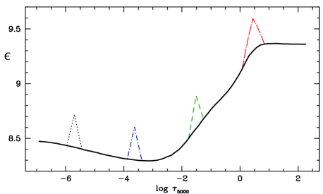
Figure 1: The VIP based Fe stratification profile for HD 133792 is plotted as logarithm of abundance $\epsilon$ (normalised to $\log H=12.0$) versus $\log\tau_{5000}$. The selection of perturbations to this profile which underly the results presented in Fig. 2 pertain to $\log\tau=-5.701$ (dot), -3.632 (dot - short dash), -1.511 (short dash), and +0.439 (dot - long dash).

This paper addresses these questions (and a few more). A simple but realistic error analysis makes it possible to estimate the interval in optical depth over which the empirical stratification profiles are more or less well defined. Extensive numerical modelling (involving models based on cap-, ring- and cloud-like structures) is then used in the assessment of the question whether uniqueness of the abundance profiles can be attained with the methods and data presently at hand. Finally we advance ideas for a strategy that could remove some non-uniqueness of the models and lead to more reliable stratification results.

2 Empirical stratifications

From the plots presented by Ryabchikova (2008) in her review which are based on results for magnetic and non-magnetic Ap stars taken from recent literature, it emerges that practically all empirical profiles correspond to a step-function described by 4 parameters, viz. the abundance in the upper atmosphere, the abundance in the deep layers, the position of the jump and the width of the jump. These stratification profiles have always been assumed to remain constant over the star, regardless of the strength of the stellar magnetic field. It is true that in stars with weak fields profiles do not depend on magnetic latitude over large parts of the stellar atmosphere – in a 1 kG horizontal field Alecian & Stift (2007) have found differences compared to the zero field case only for $\log\tau_{\rm 5000}<-3$ – but globally constant profiles can certainly not be expected at 10 or 20 kG as, for example, encountered in HD 144897 and in HD 66318. Notice that for elements having very low abundances, such as the rare earths in most stars, radiative accelerations generally exceed gravity by a considerable amount (this is due to the fact that absorption lines are completely unsaturated and remain unsaturated even for relatively strong element enhancements). In stable atmospheres, these elements then experience very high diffusion velocities and will be expelled from the star, except if they are blocked by a magnetic field. This generally occurs high up in the atmosphere ($\log\tau<-3$) in places where magnetic field lines are horizontal (Alecian & Stift, 2009, in preparation) and holds true even for weak magnetic fields. Evidence for the existence of increased Nd abundances above $\log\tau=-3.5$ in $\gamma$ Equ and in HD 24712 presented by Mashonkina, Ryabchikova & Ryabtsev (2005) is certainly not at variance with the theoretical prediction and so even for the 1 kG case one should expect significant horizontal differences in the vertical stratifications of some ions.

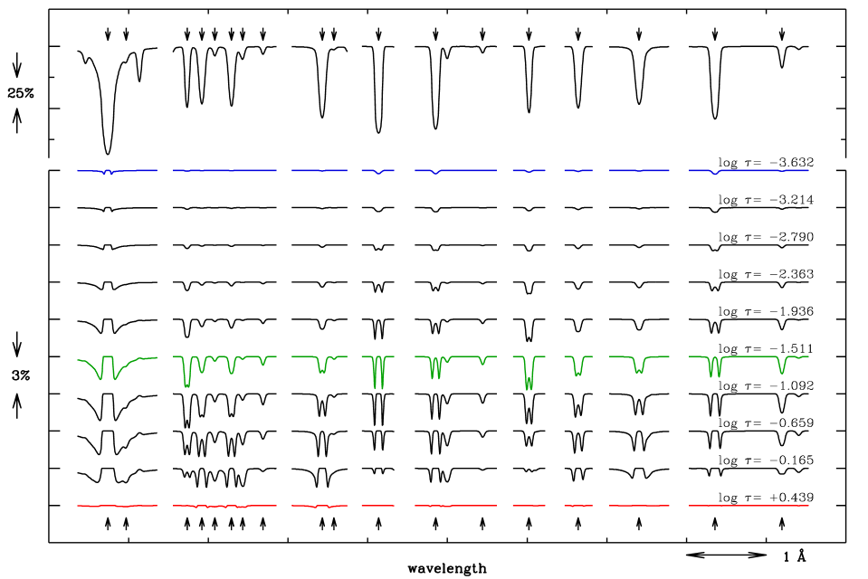
Figure 2: Lower part: The response of 19 Fe lines (indicated by arrows and listed in Table 1) to perturbations of the abundance profile of KTR06 at a given optical depth. The effect of the 0.3 dex perturbation – see text and Fig. 1 for details – is given in the sense perturbed minus unperturbed Stokes $I$. Upper part: The unperturbed spectrum with the Fe lines.

We do not want to deny that many of the stratification profiles presented in recent times lead to improved fits to the observed Stokes $I$ spectra, compared to an assumed constant abundance with depth. But it is also a fact that none of the predicted spectra are perfect, that residuals of 1-5% in normalised intensity – sometimes almost 10% – persist and that we stumble over lines where a stratified abundance gives a less satisfactory fit than a constant abundance. In the particularly well-studied star HD 133792, for example, 3 out of 7 strontium lines belong to this category, and 5 out of 26 chromium lines. In the same star, the stratification of calcium has essentially been derived from just 3 lines, one of which is still rather poorly fitted by the stratification profile. Is it possible to guarantee the uniqueness of a solution when the uncertainties in the atmospheric parameters, the limited accuracy of the atomic data, and in some cases also the unknown magnetic geometry of the star are kept in mind? Are the residuals due to the imperfect data or rather to the imperfect (and even possibly erroneous) stratification profiles?

In order to assess the question of the uniqueness of empirical stratification profiles it is imperative to first carry out a meaningful error analysis. Since HD 133792 is the star for which the most detailed, and in a certain sense, the most sophisticated, determination of stratification profiles has ever been attempted, the VIP based stratification profiles of this star are certainly well suited for this purpose.

2.1 Error analysis of the VIP

The stratification profiles for HD 133792 have been determined by KTR06 under the assumptions of constancy and maximum smoothness. Their observations extend over 10 minutes and cover just 1 phase. The quality of the fit to the observed spectrum varies between the elements. Differences between observed and predicted spectra reach some 2% in about 10 of the 28 iron lines analysed (we made these estimates from the figures). The centres of weak lines are affected to the same extent as the centres of much stronger lines; we also note that not all fits to line wings are fully satisfactory. The other elements do not fare quite so well; whereas residuals can attain 5% for Mg and Ca and 6% for Si 6%, they exceed 9% for Sr.

ion	$\lambda$	$\mid$	ion	$\lambda$	$\mid$	ion	$\lambda$
Fe 2	5018.440	$\mid$	Fe 1	5022.931	$\mid$	Fe 1	5434.524
Fe 2	5018.669	$\mid$	Fe 1	5023.186	$\mid$	Fe 2	5567.842
Fe 1	5022.236	$\mid$	Fe 2	5030.630	$\mid$	Fe 2	5961.705
Fe 1	5022.420	$\mid$	Fe 2	5030.778	$\mid$	Fe 2	6149.258
Fe 1	5022.583	$\mid$	Fe 1	5269.537	$\mid$	Fe 2	6150.098
Fe 1	5022.789	$\mid$	Fe 2	5325.553	$\mid$
Fe 1	5022.792	$\mid$	Fe 1	5326.142	$\mid$

Table 1: The iron lines shown in Fig. 2, listed with increasing wavelength and indicated (from left to right) by arrows in the figure.

At this point we shall not question the atmospheric model which could conceivably be of different effective temperature and gravity (Cowley, private communication), we neither question nor even take into consideration the magnetic field strength and geometry, we just take the published atmospheric parameters and the stratification profiles at face value. Sr is omitted in our investigation because of the exceptionally large residuals, but for the remaining elements we first calculate the reference line spectrum predicted from the published stratification profiles. Then, in a controlled experiment, we determine just how large perturbations to these abundance profiles would have to be to lead to 1% or 5% deviations from the reference line spectrum. This in turn allows us to judge the significance of any detailed structure in the stratification profiles and makes it possible to estimate the interval over which these profiles are well defined. It is not surprising – in view of the assumptions underlying the VIP approach – that there is little such structure and that the remarkable smoothness of the empirical stratifications of Mg, Si, Ca, Cr and Fe (see Fig. 5 of KTR06) is only slightly perturbed by humps or dips. The occurrence of gradients in the stratification profiles for $\log\tau_{\rm 5000}>1$ however constitutes a major puzzle, given the basic physics of radiative transfer (see section 2.1.3 for a detailed discussion).

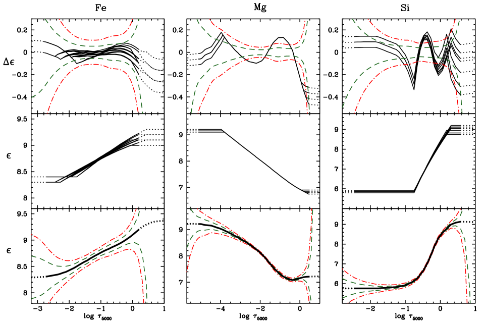
Figure 3: Bottom panels: Estimated uncertainties in the stratification curves of Fe, Mg, and Si. The dashed curves correspond to a $\pm 0.5$% maximum response to the perturbation in the spectrum, the dot-dashed curves to a $\pm 1$% maximum response. The full lines are the respective original curves digitised from KTR06; they are plotted with dots where the 1% confidence intervals become larger than 0.5 dex. Minor wiggles as in the case of Fe are due to imperfect digitisation. Middle panels: Possible alternative stratifications for which the synthetic spectra do not differ by more than 0.002 - 0.003 (rms) and by less than 0.01 (maximum) from the spectra synthesised with the respective original stratification curves. Top panels: The same alternative stratifications plotted in the sense alternative minus original profile. The respective dashed and dot-dashed curves correspond to the confidence intervals displayed in the bottom panels.

2.1.1 The tools

We chose a straightforward approach consisting in the application of a simple perturbation to the published stratification profiles. The Atlas12 code (Kurucz 2005) was used to establish an atmospheric model for HD 133792 with $T_{\rm eff}=9400$ K, $\log g=3.80$ and solar metal abundances increased by 0.5 dex. This does not constitute a perfect match to the model established by KTR06 but is largely sufficient for our purposes. This model atmosphere – with 99 layers – was then used in the COSSAM polarised spectral synthesis code (Stift 1998, 2000; Wade et al. 2001) to establish theoretical spectra covering all the lines used by KTR06. The atomic line data were taken from the VALD database (Piskunov et al. 1995; Kupka et al. 1999). The public version of COSSAM provides solely a spatial integration grid centred on the line of sight and covering the visible hemisphere of the star, but for the present calculations we employed a corotating grid (Stift 1996) largely identical to those in general use in Doppler mapping (see Voigt, Penrod & Hatzes 1987 for details). Taking the said 99 layer Atlas12 model for HD 133792, a 5-layer perturbation of {0.1 0.2 0.3 0.2 0.1} dex was added to the empirical Fe profile of KTR06 (see Fig. 1) and a {0.2 0.4 0.6 0.4 0.2} dex perturbation to the stratification profiles of the other elements. Applying these perturbations in turn to all depth points, we determined the difference between original and perturbed spectrum. Fig. 2 displays these differences for a selection of 19 Fe lines and for 10 different points in optical depth. For the 0.3 dex perturbation to the iron stratification – which corresponds to 1/3 of the total amplitude claimed by KTR06 and which is illustrated in Fig. 1 – the maximum effect on the normalised spectrum is of the order of 3%. As expected, in the deeper layers the wings of strong lines provide most of the abundance information whereas in the upper layers this is mostly done by the line cores. Outside the interval $-2.5<\log\tau_{\rm 5000}<-0.20$ the spectral response does not even reach 1%, dropping rapidly below 0.5% for $-2.9<\log\tau_{\rm 5000}$ and for $\log\tau_{\rm 5000}>0.0$. In other words, any attempt to reconstruct the Fe stratification profile beyond these limits cannot possibly yield meaningful results, simply because for the particular atmosphere in question and the abundance profile on which our calculations are based, the selected Fe lines become insensitive to abundance changes.

2.1.2 Confidence intervals

The lower panels of Figs. 3a-c show “confidence intervals” – as derived with the above mentioned perturbative approach – for the stratification curves of Fe, Mg, and Si. These confidence intervals must not be confounded with those derived from rigorous statistics but result from the simple inversion of the relation perturbation vs. maximum response obtained from our calculations. A 0.5% maximum response of the normalised spectrum requires a perturbation whose size is given by the distance between the dashed lines and the original profile. The perturbation necessary for a 1% maximum response is reflected by the dot-dashed lines. It transpires from these results that the stratification profiles are well defined over relatively narrow intervals in optical depth – here they are good to 0.1 dex in the Fe case, and good to 0.2 dex in the other cases – but become essentially undefined for $\log\tau_{\rm 5000}>+0.6$. The narrowest such intervals with less than 3 decades in optical depth are found for Fe and for Si, the Mg profile is defined over about 4 decades.

We very carefully checked that the vertical resolution of the atmospheric model is good enough so that the response curves are not affected by numerical problems. For that purpose, the same analysis was carried out with a 199 layer Atlas12 model and a 9-layer perturbation, yielding essentially identical results.

2.1.3 Assumptions and artefacts

We have seen from Figs. 3a-c that the portions of the abundance profiles below $\log\tau_{\rm 5000}=+0.6$ are invariably esentially undefined. Still, gradients in the plotted abundance profiles for Fe, Si, Sr and Ca are clearly visible beyond $\log\tau_{\rm 5000}=2.0$ in Figs. 3a and 5 of KTR06 and the question arises as to whether these have to be considered real or whether they rather constitute artefacts. From the formal solution of the radiative transfer equation the answer is unequivocally in favour of the latter: the contribution to the emerging intensity of the source function in the deepest layers multiplied by a factor of $\exp(-200)$ is tens of decades smaller than the contribution from the region near $\log\tau_{\rm 5000}=0.0$.

In the classical step-function fitting procedure a transition region connects the respective lower and upper parts of the atmosphere which exhibit different constant abundances. Self-consistent diffusion models (LeBlanc & Monin 2004) display a similar structure. The VIP method instead starts with a constant abundance throughout the star and attempts to derive deviations from this mean abundance. Such profiles – which converge to the same abundance value deep in the atmosphere and in the outermost layers, and which simply deviate from this value in some intermediate zone – are neither in accord with the theoretical models of LeBlanc & Monin (2004) nor with equilibrium solutions in the presence of magnetic fields presented by Alecian & Stift (2007, 2008). The mentioned theoretical results are also at variance with the extreme smoothness of the stratification profiles. Disturbingly, Fig. 3a of KTR06 shows that asymptotically their solution joins the mean abundance. A large regularisation parameter can make this asymptotic behaviour less visible, but it still persists and is readily visible in Fig. 5 of KTR06. Choosing the regularisation parameter such that one arrives at more or less the same solution in the interval $-4.0<\log\tau_{\rm 5000}<0.5$ irrespective of the initial abundance guess (called ’optimum regularisation’ by KTR06) constitutes a constraint that stabilises the solution but is not based on any physical considerations. Such a procedure surely smoothes out spurious structure in the profiles and effectively hides the undesirable asymptotic behaviour in the deepest layers, but there is no way to assess to what degree this might result in unwarranted and potentially severe smearing out of the abundance jump.

It should also be mentioned that a basic assumption underlying all empirical approaches so far towards the derivation of abundance stratifications in Ap stars, i.e. the insensitiveness of diffusion to magnetic fields, appears to be in serious contradiction with established theoretical wisdom. It has been shown already by Alecian & Vauclair (1981) that strong horizontal magnetic fields do have an impact on diffusion in stellar atmospheres. Even in a field of only 1 kG, stratification profiles start to depend on field direction for $\log\tau_{\rm 5000}<-3$, see Fig. 3 of Alecian & Stift (2007). So nobody can reasonably exclude that despite the rather moderate field of HD 133792, the outer parts of the stratification profiles of Sr, Ca, and Mg may be affected. And certainly one should not overlook the studies by Kurtz, Elkin & Mathys (2005) which suggest a concentration of rare earth elements at $\log\tau_{\rm 5000}=-4$ and higher in the atmosphere. In general, as Alecian & Stift (2008) have shown, equilibrium stratifications are quite sensitive to strong ($>5$ kG) magnetic fields as found in $\beta$ CrB, $\gamma$ Equ, HD 144897, and HD 66318 to mention just a few of the well-studied stars. In this context it should always be kept in mind that it is not the 2-fold difference in field strength between pole and equator in a dipolar oblique rotator model that is decisive, but the direction of the field. Results based on Zeeman Doppler mapping which suggest that abundance anomalies are related to the magnetic field topology (see e.g. Kochukhov et al. 2002) are certainly in qualitative accord with theoretical findings.

3 Uniqueness of empirical stratifications

The claim that a model derived with the “optimum regularisation” is unique has to be understood in the sense that it is unique within the framework of VIP (Kochukhov, private communication). These seems to be a reasonable claim, but we really want to have a look at the uniqueness of empirical stratification profiles in a more general sense. Looking at HD 133792, are there other abundance profiles that reproduce the observed spectrum as well as the VIP solution? Faced with an infinity of possible profile shapes and profile distributions, we started with the simplest case, viz. a step function whose shape stays constant over the star, irrespective of magnetic latitude.

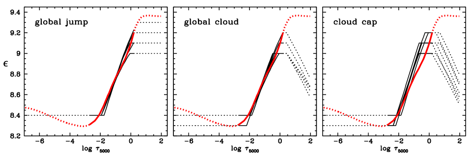
Figure 4: (a) The smooth original digitised VIP stratification curve for Fe together with a selection of global polygonal curve step-function alternatives. The curves are plotted with dots where the confidence interval exceeds 0.5 dex (as explained in Fig. 3). (b) The same for global cloud models and (c) for clouds confined to a polar cap.

A 4 parameter step function is defined by the “outer” and the “inner” abundances, and by the position and width of the transition region which connects the “inner” and the “outer” parts. We made a reasonably extended, almost exhaustive search for such step functions in the case of Mg, Si, Ca, and Fe, by calculating a dense grid covering all possible parameter values. Step function solutions were considered acceptable whenever the rms deviation of the alternative spectrum from the normalised spectrum calculated with the VIP solution did not exceed $0.002-0.003$ and when the maximum deviation was less than 1%. Given the 2 - 6% maximum size of the residuals of the VIP fits for the elements in question, this is indeed an extremely strong constraint. The middle panels of Figs. 3a-c display a selection of acceptable global step function solutions. For clarity they are plotted again in the top panels in the sense alternative minus VIP solution, and in addition, confidence intervals overlay the curves. At this point we want to remind the reader again that we are in no way looking for alternative fits to the real observed spectrum, but only for excellent fits to the VIP based synthetic spectrum. So one would not expect the alternative stratifications to differ completely from the VIP profiles.

In the case of Fe, the differences between step function solutions and the VIP curve tend to stay within the 0.5% response curve. Still, for the large number of acceptable step function models we find a noticeable spread in amplitude and also in the width of the transition region, due to the virtual lack of response to perturbations for $\log\tau_{\rm 5000}>0.2$. It thus becomes impossible to determine by line-profile fitting where deep in the atmosphere the transition region for Fe ends. But, as so often in the diagnosis of stellar atmospheres, seismology might possibly offer some hope for the future. Mg and Si do not exhibit quite the same simple behaviour, and differences between the respective alternative step function models and the original curves extend consistently and sometimes substantially beyond the 1% curves. Compared to the mean amplitude and to the mean transition region width of the alternative profiles for Mg, the spread in these quantities is relatively small; this spread becomes slightly more important for Si.

These findings confirm the correctness of our conjecture that not even for a spectrum fit at the 0.5% accuracy level can a unique model be guaranteed: neither does a 0.3 dex spread in the Fe abundances near the bottom of the atmosphere influence the fit to the spectrum, nor does a 0.6 dex amplitude give less satisfactory results than the 1.05 dex VIP amplitude.

3.1 Clouds, caps and rings

Many more simple abundance profiles can be explored which constitute a zero-order approximation to equilibrium stratification profiles found for magnetic stellar atmospheres. We decided to have a look at one particular family of models which are based on the assumption that a cloud of increased elemental abundance hovers somewhere in the atmosphere. This cloud is either distributed uniformly all over the star, or restricted to a cap around one magnetic pole, or located in a ring around the magnetic equator. There are 2 transition regions, one towards the upper part of the atmosphere, the second towards the bottom, outside of which the abundance is constant and not necessarily solar. As it turns out, all these geometries can lead to excellent fits to the VIP based synthetic spectrum. Figs. 4a-c compare the VIP iron profile to global step-function (jump) solutions as discussed above, to global cloud models, and to clouds confined to a polar cap. In all 3 classes of models shown, the abundances in the deeper layers are not particularly well defined, in contrast to the abundances in the outer layers. In the global step-function case (Fig. 4a) the 0.3 dex spread in abundances at the bottom of the atmosphere corresponds to a remarkable 50% of the minimum possible value of the jump; in the cases of a global cloud (Fig. 4b) and of a cloud in a polar cap (Fig. 4c) the spread at the bottom reduces to 0.2 dex – the minimum amplitude remaining at 0.6 dex. For the ring case we only dispose of a few hundred models and therefore it is not possible to give definitive values for the total possible spread in amplitude.

We did not delve into an exhaustive search for cap models at all possible phases but concentrated on cap models seen pole-on and on ring models seen equator-on. In both cases we found a rather narrow range of extensions, caps covering the star up to $50-60\degr$ from one magnetic pole, and rings being confined to $25-35\degr$ from the magnetic equator. Cap solutions consistently give narrower transition regions than both global step-function and global cloud solutions; for a given optical depth, the abundance is substantially higher in the interval $-1.5<\log\tau_{\rm 5000}<0$ (compare Figs. 4ab to Fig. 4c). This behaviour seems to be followed by the existing ring solutions.

Comparison of the VIP amplitude of about 1.05 dex with the maximum possible amplitude of 0.9 dex (global step-function case) or 0.8 dex (cloud cases) and with the minimum possible amplitude of 0.6 dex – in conjunction with the remarkable spread in abundance at the bottom of the atmosphere – reveals just how uncomfortably large the uncertainties in the empirical profiles really are.

4 Conclusions

On a positive note, our modelling confirms that it is possible to unequivocally establish the presence of chemical stratifications and that the sense of the abundance change is always clear. There can be thus no doubt that the decrease with depth of the Mg abundance in HD 133792, for example, is indeed a decrease, and that the abundance of Fe increases with depth in this star. The respective orders of magnitude of the abundance jumps are quite well defined.

Our findings however reveal that none of the presently used approaches is capable of providing unique stratification profiles. Taking the slowly rotating Ap star HD 133792, we have shown that for several chemical elements, many different global step-function-like solutions can be found which perfectly reproduce the VIP based synthetic spectrum; the respective amplitudes of the jumps however can differ substantially among each other. For Fe the step-function amplitudes are invariably smaller than the VIP value. We have further shown that the quality of the VIP fit is also well-matched by either global cloud-like solutions, by clouds in a cap around a magnetic pole or by clouds in a ring about the magnetic equator. Both for cap and ring models, we find a certain spread in amplitudes and in addition a narrowing of the transition region. Even when, as in the case of HD 133792, profiles of 28 Fe lines are used in the inversion, there appears to be no way to distinguish between the various possible stratification profiles (at least not with Stokes $I$ only).

Cap and ring geometries can be seen as rough approximations to the results of equilibrium stratification calculations by Alecian & Stift (2008) who have demonstrated that in magnetic fields of 5 kG and more, stratification profiles become strongly dependent on the field angle. While we consider that in strongly magnetic stars like HD 66318 and HD 144897 these models could possibly come slightly closer to reality than models which assume globally constant profile shapes, nobody can guarantee uniqueness or even correctness. Only with excellent phase coverage instead of observations at just 1 phase, and with high quality observations in all 4 Stokes parameters will it perhaps become possible to distinguish between the rival models. Ideally one would have to reconstruct the run of abundance with depth and the magnetic field vector at each point of the stellar surface. Whether such an extremely ill-defined problem can ever be solved is hard to predict.

Thus, at present, surveys of (magnetic) Ap stars in view of empirically establishing the extent of the stratification phenomenon are invaluable for our understanding of radiatively driven diffusion and its dependence on stellar parameters including magnetic fields. Empirical inversions reveal the sense and the order of magnitude of an abundance change with depth, but not the exact amplitude, nor the precise location of the transition region, and certainly not any fine structure in the stratification profile. Usually empirical stratifications are only defined over a rather restricted interval in optical depth, apparently never beyond $\log\tau_{\rm 5000}>+0.6$, and for the reasons discussed above, they are expected to be particularly unreliable in strongly magnetic Ap stars. They cannot therefore in the foreseeable future provide the desired strong constraints to theoretical diffusion modelling.

References

- [] Alecian G., 1982, A&A, 107, 61
- [] Alecian G., Vauclair S., 1981, A&A, 101, 16
- [] Alecian G., Stift M.J., 2006, A&A, 454, 571
- [] Alecian G., Stift M.J., 2007, A&A, 475, 659
- [] Alecian G., Stift M.J., 2008, CoSka, 38, 113
- [] Babel J., Michaud G., 1991, ApJ, 366, 560
- [] Babel J., Michaud G., 1991, A&A, 241, 493
- [] Borsenberger J., Praderie F., Michaud G., 1981, ApJ, 243, 533
- [] Deutsch A.J. 1958, in Lehnert B., ed, Proc. IAU Symp. 6, Electromagnetic Phenomena in Cosmical Physics. Cambridge, Cambridge Univ. Press, p. 209
- [] Kochukhov O., Piskunov N., Ilyin I., Ilyina S., Tuominen I., 2002, A&A, 389, 420
- [] Kochukhov O., Tsymbal V., Ryabchikova T., Makaganyk V., Bagnulo S., 2006, A&A, 460, 831
- [] Kupka F., Piskunov N.E., Ryabchikova T.A., Stempels H.C., Weiss W.W., 1999, A&AS 138, 119
- [] Kurtz D.W., Elkin V.G., Mathys G., 2005, MNRAS, 358, L6
- [] Kurucz R.L., 2005, MSAIS, 8, 14
- [] LeBlanc F., Monin D., 2004, in Zverko J., Ziznovsky J., Adelman S.J., Weiss W.W., eds, Proc. IAU Symp. 224, The A-Star Puzzle. Cambridge, Cambridge Univ. Press, p. 193
- [] Mashonkina L., Ryabchikova T., Ryabtsev A., 2005, A&A, 441, 309
- [] Michaud G., 1970, ApJ, 160, 641
- [] Piskunov N.E., Kupka F., Ryabchikova T.A., Weiss W.W., Jeffery C.S., 1995, A&AS 112, 525
- [] Pyper D.M., 1969, ApJS, 18, p.347
- [] Ryabchikova T., 2008, CoSka, 38, 257
- [] Stift M.J., 1996, in Strassmeier G., Linsky J.L., eds, Proc. IAU Symp. 176, Stellar surface structure. Kluwer, Dordrecht, p. 61
- [] Stift, M.J., 1998, in Asplund L., ed, Proc. Reliable Software Technologies – Ada Europe ’98. Lecture Notes in Computer Science, 1411, 128
- [] Stift M.J., 2000, A Peculiar Newsletter, 33, 27
- [] Vogt S.S., Penrod G.D., Hatzes A.P., 1987, ApJ, 321, 496
- [] Wade G.A., Bagnulo S., Kochukhov O., Landstreet J.D., Piskunov N., Stift M.J., 2001, A&A, 374, 265