Lorenz like flows: exponential decay of correlations for the Poincaré map, logarithm law, quantitative recurrence

Abstract.

In this paper we prove that the Poincaré map associated to a Lorenz like flow has exponential decay of correlations with respect to Lipschitz observables. This implies that the hitting time associated to the flow satisfies a logarithm law. The hitting time $\tau_{r}(x,x_{0})$ is the time needed for the orbit of a point $x$ to enter for the first time in a ball $B_{r}(x_{0})$ centered at $x_{0}$, with small radius $r$. As the radius of the ball decreases to $0$ its asymptotic behavior is a power law whose exponent is related to the local dimension of the SRB measure at $x_{0}$: for each $x_{0}$ such that the local dimension $d_{\mu}(x_{0})$ exists,

$$\lim_{r\rightarrow 0}\frac{\log\tau_{r}(x,x_{0})}{-\log r}=d_{\mu}(x_{0})-1$$

holds for $\mu$ almost each $x$. In a similar way it is possible to consider a quantitative recurrence indicator quantifying the speed of coming back of an orbit to its starting point. Similar results holds for this recurrence indicator.

1. Introduction

It is well known that in a chaotic dynamics the pointwise, future behavior of an initial condition is unpredictable and even impossible to be described by using a finite quantity of information. On the other hand many of its statistical properties are rather regular and often described by suitable versions of classical theorems from probability theory: law of large numbers, central limit theorem, large deviations estimations, correlation decay, hitting times, various kind of quantitative recurrence and so on.

In this article we consider a class of flows which contain the celebrated Geometric Lorenz flow and we will study some of its statistical features by a sharp estimation for the decay of correlations of its first return map on a suitable Poincaré section. This will give a quantitative recurrence estimation and an estimation for the scaling behavior of the time which is needed to hit small targets (logarithm law).

Let $\Phi^{t}$ be a $C^{1}$ flow in ${\mathbb{R}}^{3}$. Quantitative recurrence estimations and logarithm laws can be seen in the following framework: we are interested in a quantitative estimation of the speed of approaching of a certain orbit $\Phi^{t}(x)$ (starting from the point $x$) of the system to a given target point $x_{0}$. Let $B_{r}(x_{0})$ be a ball with radius $r$ centered at $x_{0}$. We consider the time

$$\tau_{r}(x,x_{0})=\inf\{t\in\mathbb{R}^{+}:\Phi^{t}(x)\in B_{r}(x_{0})\}$$

needed for the orbit of $x$ to enter in $B_{r}(x_{0})$ for the first time and the asymptotic behavior of $\tau_{r}(x,x_{0})$ as $r$ decreases to $0$. Often this is a power law of the type $\tau_{r}\sim r^{-d}$ and then it is interesting to extract the exponent $d$ by looking at the behavior of

(1) $$R(x,x_{0})=\underset{r\rightarrow 0}{\lim}\frac{\log\tau_{r}(x,x_{0})}{-\log r}.$$

In this way, we have a hitting time indicator for orbits of the system.

If the orbit $\Phi^{t}$ starts at $x_{0}$ itself and we consider the second entrance time in the ball

(2) $$\tau_{r}^{\prime}(x_{0})=\inf\{t\in\mathbb{R}^{+}:\Phi^{t}(x_{0})\in B_{r}(x_{0}),\exists i<t,s.t.\Phi^{i}(x_{0})\notin B_{r}(x_{0})\}$$

(because the orbit trivially starts inside the ball) with the same construction as before, we have a quantitative recurrence indicator. If the dynamics is chaotic enough, often the above indicators converge to a quantity which is related to the local dimension of the invariant measure of the system and in the hitting time case this relation is called logarithm law.

Hitting time results of this kind (sometime replacing balls with other suitable target sets) have been proved in many continuous time dynamical systems of geometrical interest: geodesic flows, unipotent flows, homogeneous spaces, etc. (see e.g. [6, 20, 23, 38, 30, 32]). For discrete time systems this kind of results hold in general if the system has fast enough decay of correlation ([16]). Mixing is however not sufficient, since this relation does not hold in some slowly mixing system having particular arithmetical properties ([18]). Some further connections with arithmetical properties are shown in interesting examples as rotations and interval exchange maps (see e.g. [14, 21, 22]). This kind of problem is also connected with the so called dynamical Borel Cantelli results (see [17] and e.g. [41, 20, 17, 13]). Moreover, in the symbolic setting, similar results about the hitting time are used in information theory (see e.g. [37, 24]). About quantitative recurrence, our approach follows a set of results connecting a quantitative recurrence estimation with local dimension (see e.g. [36, 35, 7, 9]). We remark that the speed of correlation decay for Lorenz like flows is not yet known (although some are proved to be mixing, see [29]) hence quantitative recurrence and hitting time results cannot be proved directly using this tool, instead of this we will consider a Poincaré section, estimating its correlation decay and work with return times.

1.1. Statement of results

Let $I=[-\frac{1}{2},\frac{1}{2}]$ be a unit interval, we consider a flow $X^{t}$ on $\mathbb{R}^{3}$ having a Poincaré section on a square $\Sigma=I\times I$ satisfying the following properties:

1):

The flow induces a first return map $F:\Sigma\rightarrow\Sigma$ of the form $F(x,y)=(T(x),G(x,y))$ (preserves the natural vertical foliation of the square) and:

1.a):

There is $c\in I$ and $k\geq 0$ such that, if $x_{1},x_{2}$ are such that $c\notin[x_{1},x_{2}]$ then $\forall y\in I:|G(x_{1},y)-G(x_{2},y)|\leq k\cdot|x_{1}-x_{2}|$

1.b):

$F|_{\gamma}$ is $\lambda$-Lipschitz with $\lambda<1$ (hence is uniformly contracting) on each vertical leaf $\gamma$: $|G(x,y_{1})-G(x,y_{2})|\leq\lambda\cdot|y_{1}-y_{2}|$

1.c):

$T:I\rightarrow I$ is onto and piecewise monotonic, with two $C^{1}$ increasing branches on the intervals $[-\frac{1}{2},c)$,$(c,\frac{1}{2}]$ and $T^{\prime}>1$ where it is defined. Moreover $\underset{x\rightarrow c^{-}}{\lim}T(x)=\frac{1}{2},T(c)=-\frac{1}{2},$ $\underset{x\rightarrow c}{\lim}T^{\prime}(x)=\infty$.

1.d):

$\frac{1}{|T^{\prime}|}$ has bounded variation.

By the statistical properties of the map $T$, which is piecewise expanding, under the above assumptions, it turns out that $F$ has a unique SRB measure $\mu_{F}.$ We then ask the following property for the flow:

2):

The flow $X^{t}$ is transversal to the section $\Sigma$ and its return time to $\Sigma$ is integrable with respect to $\mu_{F}$.

In Section 2.1 we will describe the geometric Lorenz system and we show that it satisfies these properties.

The main results of the paper concern some statistical properties of $X^{t}$ and $F$, more precisely:

Theorem A (decay of correlation for the Poincaré map) The unique SRB measure $\mu_{F}$ of $F$ has exponential decay of correlation with respect to Lipschitz observables.

This result is proved in Section 4 (Theorem 4.7) where the reader can also find a precise definition of correlation decay. The proof also uses a regularity estimation for the invariant measure $\mu_{F}$ which can be found in the Appendix I (Lemma 8.1) and is proved by sort of Lasota-Yorke inequality. We remark that a stretched-exponential bound for the decay of correlation for a two dimensional Lorenz like map was given in [12] and [2].

We say that a point $x_{0}\in{\mathbb{R}}^{3}$ is regular if there are $y_{0}\in\Sigma$ and $t_{0}\geq 0$ such that $X^{t_{0}}$ induces a diffeomorphism between a neighborhood of $y_{0}$ and a neighborhood of $x_{0}$.

In Section 3 we recall how to construct an SRB ergodic invariant measure for the flow $X^{t}$ which will be denoted by $\mu_{X}$. It turns out that this measure has the following property

Theorem B (logarithm law for the flow) For each regular $x_{0}$ such that the local dimension $d_{\mu_{X}}(x_{0})$ is defined it holds

(3) $$\underset{r\rightarrow 0}{\lim}\frac{\log\tau_{r}(x,x_{0})}{-\log r}=d_{\mu_{X}}(x_{0})-1$$

for a.e. starting point $x$.

This is proved in Section 6 (Theorem 6.3) and uses the above decay of correlation estimation for the first return map $F$, a result from [16] giving the hitting time estimation for systems having faster than polynomial decay of correlations and finally the integrability of return time is used to get the result for the flow.

Using the main result of [35], by a similar construction, if the flow also satisfies the following property

3):

the map $T$ has derivative bounded by a power law near $c$: there is a $\beta>0$ s.t. $(x-c)^{\beta}T^{\prime}(x)$ is bounded in a neighborhood of $c$

we prove (in Section 7, Corollary 7.4) the following estimation for the return time

Theorem C (quantitative recurrence) If the flow satisfies conditions 1),2), 3) above, then for a.e. $x$ it holds

(4) $$\underset{r\rightarrow 0}{\lim\sup}\frac{\log\tau_{r}^{\prime}(x)}{-\log r}=\overline{d}_{\mu_{X}}(x)-1,\quad\underset{r\rightarrow 0}{\lim\inf}\frac{\log\tau_{r}^{\prime}(x)}{-\log r}=\underline{d}_{\mu_{X}}(x)-1.$$

In the Appendix II we give an auxiliary result, using a theorem by Steinberger [40] showing that the local dimension is defined a.e. for the Geometric Lorenz system.

2. Geometric Lorenz model

In this section we will introduce and motivate the so-called Geometric Lorenz system. This is the main example where our results will be applied. Indeed we will see that assumption 1.a),…,1.d) and 2) of the introduction are verified for this model. The results in this section are however not strictly necessary for the proofs of our main theorems. The reader familiar with the construction of such models can skip it and start at Section 3.

In 1963 the meteorologist Edward Lorenz published in the Journal of Atmospheric Sciences ([27]) an example of a parametrized $2$-degree polynomial system of differential equations

$$\dot{x} =a(y-x) a=10$$

(5) $$\dot{y} =rx-y-xz r=28$$

$$\dot{z} =xy-bz b=8/3$$

as a very simplified model for thermal fluid convection, motivated by an attempt to understand the foundations of weather forecast.

Numerical simulations performed by Lorenz for an open neighborhood of the chosen parameters suggested that almost all points in phase space tend to a chaotic attractor.

An attractor is a bounded region in phase-space, invariant under time evolution, such that the forward trajectories of most (positive probability) or, even, all nearby points converge to. And what makes an attractor chaotic is the fact that trajectories converging to the attractor are sensitive with respect to initial data: trajectories of two any nearby points get apart under time evolution.

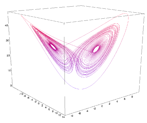
Figure 1. Lorenz chaotic attractor

Lorenz’s equations proved to be very resistant to rigorous mathematical analysis, and also presented serious difficulties to rigorous numerical study. As an example, the above stated existence of a chaotic attractor for the original Lorenz system where not proved until the year 2000, when Warwick Tucker did it with a computer aided proof (see [43, 42]).

In order to construct a class of flows having properties which are very similar to the Lorenz system and are easier to be studied, Afraimovich, Bykov and Shil’nikov [1], and Guckenheimer, Williams [19], independently constructed the so-called geometric Lorenz models for the behavior observed by Lorenz. These models are flows in $3$-dimensions for which one can rigorously prove the existence of a chaotic attractor that contains an equilibrium point of the flow, which is an accumulation point of typical regular solutions. Recall that $\gamma$ is a regular solution for the flow $X^{t}$ if $X^{t}(x)\neq x$ for all $x\in\gamma$ and $t>0$. The accumulation of regular orbits near an equilibrium prevents such sets from being hyperbolic [33]. Furthermore, this attractor is robust (in the $C^{1}$ topology): it can not be destroyed by any small perturbation of the original flow.

We point out that the robustness of this example provides an open set of flows which are not Morse-Smale, nor hyperbolic, and also non-structurally stable (see [33, 10] ).

2.1. Construction of the geometric model: near the equilibrium

The results of the paper will be given for a class of three dimensional flows which will be defined axiomatically. To show that these axioms are verified in the geometric Lorenz models we give a detailed introduction to this model.

We first analyze the dynamics in a neighborhood of the singularity at the origin, and then we complete the flow, imitating the butterfly shape of the original Lorenz flow (see Figure 1 and compare with Figure 3).

In the original Lorenz system the origin $p=0=(0,0,0)$ is an equilibrium of saddle type for the vector field defined by equations (2) with real eigenvalues $\lambda_{i}$, $i\leq 3$ satisfying

(6) $$0<\frac{\lambda_{1}}{2}\leq-\lambda_{3}<\lambda_{1}<-\lambda_{2}$$

(in the classical Lorenz system $\lambda_{1}\approx 11.83$ , $\lambda_{2}\approx-22.83$, $\lambda_{3}=-8/3$).

If certain nonresonance conditions are satisfied (see [39]) this vector field is smoothly linearizable in a neighborhood of the origin. To construct a model which is similar to the original Lorenz one we start with a linear system $(\dot{x},\dot{y},\dot{z})=(\lambda_{1}x,\lambda_{2}y,\lambda_{3}z)$, with $\lambda_{i}$, $1\leq i\leq 3$ satisfying relation (6). This vector field will be considered in the cube $[-1,1]^{3}$ containing the origin.

For this linear flow, the trajectories are given by

(7) $$X^{t}(x_{0},y_{0},z_{0})=(x_{0}e^{\lambda_{1}t},y_{0}e^{\lambda_{2}t},z_{0}e^{\lambda_{3}t}),$$

where $(x_{0},y_{0},z_{0})\in{\mathbb{R}}^{3}$ is an arbitrary initial point near $p=(0,0,0)$.

Consider $\Sigma=\big{\{}(x,y,1):|x|\leq{\frac{1}{2}},\quad|y|\leq{\frac{1}{2}}\big{\}}$ and

$$\Sigma^{-} =\big{\{}(x,y,1)\in\Sigma:x<0\big{\}}, \qquad\Sigma^{+} =\big{\{}(x,y,1)\in\Sigma:x>0\big{\}}\quad\text{and}$$

$$\Sigma^{*} =\Sigma^{-}\cup\Sigma^{+}=\Sigma\setminus\Gamma, \quad\text{where}\quad\Gamma =\big{\{}(x,y,1)\in\Sigma:x=0\big{\}}.$$

$\Sigma$ is a transverse section to the linear flow and every trajectory crosses $\Sigma$ in the direction of the negative $z$ axis.

Consider also $\tilde{\Sigma}=\{(x,y,z):|x|=1\}=\tilde{\Sigma}^{-}\cup{\tilde{\Sigma}}^{+}$ with ${\tilde{\Sigma}}^{\pm}=\{(x,y,z):x=\pm 1\}$. For each $(x_{0},y_{0},1)\in\Sigma^{*}$ the time $t$ such that $X^{t}(x_{0},y_{0},1)\in\tilde{\Sigma}$ is given by

(8) $$t(x_{0})=-\frac{1}{\lambda_{1}}\log{|x_{0}|}$$

which depends on $x_{0}\in\Sigma^{*}$ only and is such that $t(x_{0})\to+\infty$ when $x_{0}\to 0$.

Hence, using (8), we get (where $\operatorname{sgn}(x)=x/|x|$ for $x\neq 0$ )

$$X^{t(x_{0})}(x_{0},y_{0},1)=\big{(}\operatorname{sgn}(x_{0}),y_{0}e^{\lambda_{2}\cdot t(x_{0})},e^{\lambda_{3}\cdot t(x_{0})}\big{)}=\big{(}\operatorname{sgn}(x_{0}),y_{0}|x_{0}|^{-\frac{\lambda_{2}}{\lambda_{1}}},|x_{0}|^{-\frac{\lambda_{3}}{\lambda_{1}}}\big{)}.$$

Since $0<\frac{\lambda_{1}}{2}<-\lambda_{3}<\lambda_{1}<-\lambda_{2}$, we have $\frac{1}{2}<\alpha=-\frac{\lambda_{3}}{\lambda_{1}}<1<\beta=-\frac{\lambda_{2}}{\lambda_{1}}$.

Consider $L:\Sigma^{*}\to\ {\tilde{\Sigma}}^{\pm}$ defined by

(9) $$L(x,y,1)=\big{(}\operatorname{sgn}(x),y|x|^{\beta},|x|^{\alpha}\big{)}.$$

Figure 2. Behavior near the origin.

It is easy to see that $L(\Sigma^{\pm})$ has the shape of a cusp triangle without the vertex $(\pm 1,0,0)$. In fact the vertex $(\pm 1,0,0)$ are cusp points at the boundary of each of these sets. The fact that $0<\alpha<1<\beta$ together with equation (9) imply that $L(\Sigma^{\pm})$ are uniformly compressed in the $y$-direction.

Clearly each segment $\Sigma^{*}\cap\{x=x_{0}\}$ is taken by $L$ to another segment $\tilde{\Sigma}^{\pm}\cap\{z=z_{0}\}$ as sketched in Figure 2.

Figure 3. $T_{\pm}\circ R_{\pm}$ takes $\tilde{\Sigma}^{\pm}$ to $\Sigma$.

2.2. The random turns around the origin

To imitate the random turns of a regular orbit around the origin and obtain a butterfly shape for our flow, as it is in the original Lorenz flow depicted at Figure 1, we proceed as follows.

Recall that the equilibrium $p$ at the origin is hyperbolic and so its stable $W^{s}(p)$ and unstable $W^{u}(p)$ manifolds are well defined, [33]. Observe that $W^{u}(p)$ has dimension one and so, it has two branches, $W^{u,\pm}(p)$, and $W^{u}(p)=W^{u,+}(p)\cup\{p\}\cup W^{u,-}(p)$.

The sets $L(\Sigma^{\pm})$ should return to the cross section $\Sigma$ through a flow described by a suitable composition of a rotation $R_{\pm}$, an expansion $E_{\pm\theta}$ and a translation $T_{\pm}$.

The rotation $R_{\pm}$ has axis parallel to the $y$-direction. More precisely is such that $(x,y,z)\in\tilde{\Sigma}^{\pm}$, then

(13) $$R_{\pm}(x,y,z)=\left(\begin{array}[]{cccc}0&0&\pm 1\\ 0&1&0\\ \pm 1&0&0\end{array}\right).$$

The expansion occurs only along the $x$-direction, so, the matrix of $E_{\theta}$ is given by

(17) $$E_{\pm\theta}(x,y,z)=\left(\begin{array}[]{cccc}\theta&0&0\\ 0&1&0\\ 0&0&1\end{array}\right)$$

with $\theta\cdot({\frac{1}{2}}^{\alpha})<1$ and $\theta\cdot\alpha\cdot 2^{1-\alpha}>1$. The first condition is to ensure that the image of the resulting map is contained in $\Sigma$, the second condition makes a certain one dimensional induced map to be piecewise expanding. This point will be discussed below.

$T_{\pm}:{\mathbb{R}}^{3}\to{\mathbb{R}}^{3}$ is chosen such that the unstable direction starting from the origin is sent to the boundary of $\Sigma$ and the image of both $\tilde{\Sigma}^{\pm}$ are disjoint. These transformations $R_{\pm},E_{\pm\theta},T_{\pm}$ take line segments $\tilde{\Sigma}^{\pm}\cap\{z=z_{0}\}$ into line segments $\Sigma\cap\{x=x_{1}\}$ as sketched in Figure 3, and so does the composition $T_{\pm}\circ E_{\pm\theta}\circ R_{\pm}$.

This composition of linear maps describes a vector field in a region outside $[-1,1]^{3}$ in the sense that one can use the above matrices to define a vector field $V$ such that the time one map of the associated flow realizes $T_{\pm}\circ E_{\pm\theta}\circ R_{\pm}$ as a map $L(\Sigma^{\pm})\to\Sigma$. This will not be explicit here, since the choice of the vector field is not really important for our purposes (provided the return time is integrable).

The above construction allow to describe for each $t\in\mathbb{R}$ the orbit $X^{t}(x)$ of each point $x\in\Sigma$: the orbit will start following the linear field until $\tilde{\Sigma}^{\pm}$ and then it will follow $V$ coming back to $\Sigma$ and so on. Let us denote with ${\cal B}=\{X^{t}(x),x\in\Sigma,t\in\mathbb{R}^{+}\}$ the set where this flow acts. The geometric Lorenz flow is then the couple $({\cal B},X^{t})$ defined in this way.

The Poincaré first return map will be hence defined by $F:\Sigma^{*}\to\Sigma$ as

(18) $$F(x,y)=\left\{\begin{array}[]{ccc}T_{+}\circ E_{+\theta}\circ R_{+}\circ{L}(x,y,1)&\mbox{for }\,x>0\\ T_{-}\circ E_{-\theta}\circ R_{-}\circ{L}(x,y,1)&\mbox{for }\,x<0\end{array}\right.$$

The combined effects of $T_{\pm}\circ R_{\pm}$ and ${L}$ on lines implies that the foliation ${\mathcal{F}}^{s}$ of $\Sigma$ given by the lines $\Sigma\cap\{x=x_{0}\}$ is invariant under the return map. In another words, we have

$(\star)$ for any given leaf $\gamma$ of ${\mathcal{F}}^{s}$, its image $F(\gamma)$ is contained in a leaf of ${\mathcal{F}}^{s}$.

2.3. An expression for the first return map and its differential

Combining equations (9) with the effect of the rotation composed with the expansion and the translation, we obtain that $F$ must have the form

(19) $$F(x,y)=\big{(}f_{Lo}(x),g_{Lo}(x,y)\big{)}$$

where $f_{Lo}:I\setminus\{0\}\to I$ and $g_{Lo}:(I\setminus\{0\})\times I\to I$ are given by

(20) $$f_{Lo}(x)=\left\{\begin{array}[]{cccc}f_{1}(x^{\alpha})&x<0\\ f_{0}(x^{\alpha})&x>0\end{array}\right.\quad\mbox{with $f_{i}=(-1)^{i}\theta\cdot x+b_{i},i\in\{0,1\}$, and }$$

(21) $$g_{Lo}(x,y)=\left\{\begin{array}[]{cccc}g_{1}(x^{\alpha},y\cdot x^{\beta})&x<0\\ g_{0}(x^{\alpha},y\cdot x^{\beta})&x>0,\end{array}\right.\,\,$$

where $g_{1}|I^{-}\times I\to I$ and $g_{0}|I^{+}\times I\to I$ are suitable affine maps. Here $I^{-}=(-1/2,0)$, $I^{+}=(0,1/2)$.

Figure 4. $F(\Sigma^{*})$.

Figure 5. Projection on $I$.

Now, to find an expression for $DF$ we proceed as follows. Recall $F=T_{\pm}\circ E_{\pm\theta}\circ R_{\pm}\circ L$, $L$ is as in (9), $DR_{\pm}$ is as in (13). Given $q=(x,y)\in\Sigma^{*}$ with $x>0$, we have

$$DL(x,y,1)=\left(\begin{array}[]{cccc}\beta\cdot y\cdot x^{\beta-1}&x^{\beta}\\ \alpha\cdot x^{\alpha-1}&0\\ \end{array}\right).$$

Restricting the rotation and the other linear maps to $\tilde{\Sigma}^{\pm}$ and composing the resulting matrices we get

(24) $$DF(x,y)=\left(\begin{array}[]{cccc}\theta\cdot\alpha\cdot x^{(\alpha-1)}&0\\ \beta\cdot yx^{(\beta-\alpha)}&x^{\beta}\end{array}\right).$$

The expression for $DF$ at $q=(x,y)$ with $x<0$ is similar.

2.4. Properties of the map $g_{Lo}$

Observe that by construction $g_{Lo}$ in equation (18) is piecewise $C^{2}$. Moreover, equation (24) implies the following bounds on its partial derivatives :

1. For all $(x,y)\in\Sigma^{*},x>0$, we have ${\partial_{y}}g_{Lo}(x,y)=x^{\beta}$. As $\beta>1$, $|x|\leq 1/2$, there is $0<\lambda<1$ such that

   (25) $$|{\partial_{y}}g_{Lo}|<\lambda.$$

   The same bound works for $x<0$.

2. For all $(x,y)\in\Sigma^{*},x\neq 0$, we have ${\partial_{x}}g_{Lo}(x,y)=\beta\cdot x^{\beta-\alpha}$. As $\beta-\alpha>0$ and $|x|\leq 1/2$, we get

   (26) $$|\partial_{x}g_{Lo}|<\infty.$$

Item (a) above implies that the map $F=(f_{Lo},g_{Lo})$ is uniformly contracting on the leaves of the foliation ${\mathcal{F}}^{s}$: there is $C>0$ such that, if $\gamma$ is a leaf of ${\mathcal{F}}^{s}$ and $x,y\in\gamma$ then $\operatorname{dist}\big{(}F^{n}(x),F^{n}(y)\big{)}\leq{\lambda^{n}}\cdot C\cdot\operatorname{dist}(x,y)$ where $\lambda$ can be chosen as the one given by equation (25).

Figure 6. The Lorenz map $f_{Lo}$.

2.5. Properties of the one-dimensional map $f_{Lo}$

Now let us outline the main properties of $f_{Lo}$. We recall that we chosen $\theta$ such that $\theta\cdot\alpha\cdot 2^{1-\alpha}>1$.

The following properties are easily implied from the construction of $X^{t}$:

1. By equation (20) and the way $T_{\pm}$ is defined, $f_{Lo}$ is discontinuous at $x=0$. The lateral limits $f_{Lo}(0^{\pm})$ do exist, $f_{Lo}(0^{\pm})=\pm\frac{1}{2}$,

2. $f_{Lo}$ is $C^{2}$ on $I\setminus\{0\}$. By the choice of $\theta$ it holds $f^{\prime}_{Lo}(1/2)>1$. By the convexity properties of $f_{Lo}$ we then obtain that

   (27) $$f^{\prime}_{Lo}(x)>1\quad\quad\mbox{for all}\quad\quad x\in I\setminus\{0\}.$$

3. The limits of $f_{Lo}^{\prime}$ at $x=0$ are $\lim_{x\to 0}f_{Lo}^{\prime}(x)=+\infty$.

We obtain that $f_{Lo}$ is a piecewise expanding map. Moreover $f_{Lo}$ has a dense orbit, which in its turn implies that the closure of the maximal invariant set by $f_{Lo}$ is the whole interval $I$, see [5, Lemma 2.11].

Now recall that the variation $\operatorname{var}\phi$ of a function $\phi:[0,1]\to{\mathbb{R}}$ is defined by

$$\operatorname{var}\phi=\sup\sum_{i=1}^{n}|\phi(x_{i-1})-\phi(x_{i})|$$

where the supremum is taken over all finite partitions $0=x_{0}<x_{1}<\cdots<x_{n}=1$, $n\geq 1$, of $[0,1]$. The variation $\operatorname{var}_{J}\phi=\operatorname{var}(\phi|J)$ of $\phi$ over an arbitrary interval $J\subset[0,1]$ is defined by a similar expression, with the supremum taken over all the $x_{0},x_{1},\cdots,x_{n}\in J$, with $\inf J\leq x_{0}<x_{1}<\cdots<x_{n}\leq\sup J$. One says that $\phi$ has bounded variation, or $\phi$ is BV for short, if $\operatorname{var}\phi<\infty$.

The one dimensional map has the following property, which is important to obtain the existence of an SRB invariant measure and its statistical properties.

Lemma 2.1.

Let $X^{t}$ a $C^{2}$ geometric Lorenz flow as before and $f_{Lo}$ be the one-dimensional map associated to $X^{t}$. Then $\frac{1}{f_{Lo}^{\prime}}$ is BV.

Proof.

Each branch of $f_{Lo}$ is the composition of an affine map with $x^{\alpha}$ then it is a convex function. Hence, the derivative $f^{\prime}_{Lo}$ is monotonic on each branch, implying that $(f^{\prime}_{lo})^{-1}$ is also monotonic. On the other hand, $(f^{\prime}_{Lo})^{-1}$ is bounded because $f^{\prime}_{lo}>1$. Thus $(f^{\prime}_{Lo})^{-1}$ is monotonic and bounded and hence is BV. ∎

We have seen that $f_{Lo}$ is a topologically transitive piecewise expanding map with $\frac{1}{f_{Lo}^{\prime}}$ BV. The statistical properties of such maps are well known. Next we state a result about it, which will be used later:

Proposition 2.2.

([44], Prop.3.8) The one-dimensional $f_{Lo}$ admits a unique invariant probability $\mu_{f_{Lo}}$ which is absolutely continuous with respect to Lebesgue measure $m$, it is ergodic and so a SRB measure for the map. Moreover $d\mu_{f_{Lo}}/dm$ is a BV function and in particular it is bounded. Furthermore $f_{Lo}$ has exponential decay of correlations for $L^{1}$ and BV observables and any a.c.i.m. converges exponentially fast to the invariant measure: there are constants $C>0$ and $\lambda>0$, depending on the system such that for each $n$ and observables $f,g$:

$$\left|\int~{}g(F^{n}(x))f(x)dm-\int g(x)d\mu\int f(x)dm\right|\leq C\cdot\|g\|_{L_{1}}\cdot\|f\|_{BV}\cdot e^{-\lambda n}.$$

Summarizing, for what it was said above, the study of the $3$-flow can be reduced to the study of a bi-dimensional map $F$. Moreover, the dynamics of this map can be further reduced to a one-dimensional map, $f_{Lo}$ called one dimensional Lorenz map. Figure 6 shows the graph of this one-dimensional transformation, and Figure 5 sketches $F(\Sigma^{*})$.

3. A physical measure for a Lorenz like flow

In this section, following [44] we construct a physical measure for a flow $X^{t}$ which satisfies the assumptions 1a),…,1d),2) in the introduction. As noticed in the previous section, these assumptions 1a),…,1d) are satisfied by the Geometric Lorenz system.

Properties 1a),…,1d) implies that the flow Poincaré map has an invariant foliation and the one dimensional induced map $T$ is piecewise expanding. Piecewise expanding maps (see Proposition 2.2) admits a unique invariant probability measure $\mu_{T}$ which is absolutely continuous with respect to Lebesgue measure $m$.

From $\mu_{T}$ we may construct a SRB measure $\mu_{F}$, for the first return map $F$ through the following general procedure ([11, 44]). Since $\mu_{T}$ is defined on the interval $I$ which can be identified to the space of leaves of the contracting foliation ${\mathcal{F}}^{s}$, we may also think of it as a measure on the $\sigma$-algebra of Borel subsets of $\Sigma$ which are union of entire leaves of ${\mathcal{F}}^{s}$. Using the fact that $F$ is uniformly contracting on leaves of ${\mathcal{F}}^{s}$ we conclude that the sequence

$$F^{*n}(\mu_{T}),\quad n\geq 1,$$

of push-forwards of $\mu_{T}$ under $F$ is weak*-Cauchy: given any continuous $\psi:\Sigma\to{\mathbb{R}}$

$$\int\psi d(F^{n*}\mu_{T})=\int(\psi\circ F^{n})d{\mu_{T}},\quad n\geq 1,$$

is a Cauchy sequence in ${\mathbb{R}}$, see [44, pp.173]. Define $\mu_{F}$ to be the weak*-limit of this sequence, that is,

$$\int\psi d\mu_{F}=\lim\int\psi d(F^{*n}\mu)$$

for each continuous $\psi$. Then $\mu_{F}$ is invariant under $F$, and it is an ergodic physical measure for $F$. The last statement follows from the fact that $\mu_{T}$ is an ergodic physical measure for $T$, together with the fact that asymptotic time-averages of continuous functions $\psi:\Sigma\to{\mathbb{R}}$ are constant on the leaves of ${\mathcal{F}}^{s}$.

Given any point $x$ whose orbit sooner or later will cross $\Sigma$ we denote with $t(x)$ the first strictly positive time such that $X^{t(x)}(x)\in\Sigma$ (the return time of $x$ to $\Sigma$). Coherently with the Geometric Lorenz system, we will denote by $\Sigma^{*}$ the (full measure, by the assumption 1 in the introduction) subset of $\Sigma$ where $t$ is defined.

Now we show how to construct an physical invariant measure for the flow, when the return time is integrable:

(28) $$\int_{\Sigma^{*}}td\mu_{F}<\infty.$$

Denote by $\sim$ the equivalence relation on $\Sigma\times{\mathbb{R}}$ given by $(w,t(w))\sim(F(w),0).$

Let $N=(\Sigma^{*}\times{\mathbb{R}})/\sim$ and $\nu=\pi_{*}(\mu_{F}\times dt)$, where $\pi:\Sigma^{*}\times{\mathbb{R}}\to N$ is the quotient map and $dt$ is a Lebesgue measure in ${\mathbb{R}}$. Equation (29) gives that $\nu$ is a finite measure. Let $\phi:N\to{\mathbb{R}}^{3}$ be defined by $\phi(w,t)=X^{t}(w)$. Let $\mu_{X}=\phi_{*}\nu$. The measure $\mu_{X}$ is a physical for the flow $X^{t}$:

$$\frac{1}{T}\int_{0}^{T}\psi(X^{t}(w))dt\to\int\psi d\mu_{X}\quad\mbox{as}\quad T\to\infty$$

for every continuous function $\psi:{\mathbb{R}}^{3}\to{\mathbb{R}}$, and Lebesgue almost every point $w\in\phi(N).$

We end the subsection remarking that the Geometric Lorenz flow has integrable return time, hence the above construction for the invariant measure can be applied to it. As before denote by $t:\Sigma\setminus\Gamma\to(0,\infty)$ the return time to $\Sigma$. Then, recalling Equation (8) there are $K,C>0$ such that

$$-K^{-1}\log(d(x,\Gamma))-{C}\leq t(x)\leq-K\log(d(x,\Gamma))+C.$$

Combining this with the definition of $\mu_{F}$ and the remark made above that $d\mu_{f_{L}o}/dm$ is a bounded function, we conclude that

Proposition 3.1.

The return time is integrable

(29) $$t_{0}=\int td\mu_{F}<\infty.$$

3.1. Local dimension.

Let us recall the definition of local dimension and fix some notations for what follows.

Let $(M,d)$ be a metric space and assume that $\mu$ is a Borel probability measure on $M$. Given $x\in M$, let $B_{r}(x)=\{y\in M;d(x,y)\leq r\}$ be the ball centered at $x$ with radius $r$. The local dimension of $\mu$ at $x\in M$ is defined by

$$d_{\mu}(x)=\lim_{r\to 0}\frac{\log\mu(B_{r}(x))}{\log r}$$

if this limit exists. In this case $\mu(B_{r}(x))\sim r^{d_{\mu}(x)}$.

This notion characterizes the local geometric structure of an invariant measure with respect to the metric in the phase space of the system, see [45] and [34].

We can always define the upper and the lower local dimension at $x$ as

$${\overline{d}}_{\mu}(x)=\lim\sup_{r\to 0}\frac{\log\mu(B_{r}(x))}{\log r}\,,\quad\quad{\underline{d}}_{\mu}(x)=\lim\inf_{r\to 0}\frac{\log\mu(B_{r}(x))}{\log r}.$$

If $d^{+}(x)=d^{-}(x)=d$ almost everywhere the system is called exact dimensional. In this case many properties of dimension of a measure coincide. In particular, $d$ is equal to the infimum Hausdorff dimension of full measure sets: $d=\inf\{\dim_{H}Z;\mu(Z)=1\}.$ This happens in a large class of systems, for example, in $C^{2}$ diffeomorphisms having non zero Lyapunov exponents almost everywhere, [34].

3.2. Relation between local dimension for $F$ and for $X^{t}$

Let us establish a relation between $d_{\mu_{F}}$ and $d_{\mu_{X}}$ which will be used in the following.

Proposition 3.2.

Let $x\in\mathbb{R}^{3}$ and $\pi(x)$ be the projection on $\Sigma$ given by $\pi(x)=y$ if $x$ is on the orbit of $y\in\Sigma$ and the orbit from $y$ to $x$ does not cross $\Sigma$ (if $x\in\Sigma$ then $\pi(x)=x$). For all regular points $x\in\mathbb{R}^{3}$

(30) $${{\overline{d}}_{\mu_{X}}}(x)={{\overline{d}}_{\mu_{F}}}(\pi(x))+1,\ \ {{\underline{d}}_{\mu_{X}}}^{-}(x)={{\underline{d}}_{\mu_{F}}}^{-}(\pi(x))+1.$$

Proof.

First observe that for product measures as ${\mu_{X}}=\mu_{F}\times dt$, where $dt$ is the Lebesgue measure at the line, the formula is trivially verified. But, by construction $\mu_{X}=\phi_{\ast}(d\mu_{F}\times dt)$, where $\phi:{\mathbb{R}}^{3}\to{\mathbb{R}}^{3}$ is a local bi-Lipschitz map at each regular point. Since the local dimension is invariant by local bi-Lipschitz maps, it follows the required equation (30). ∎

4. Decay of correlations for two dimensional Lorenz maps

In this section we estimate the decay of correlations for a class of Lorenz like maps containing the first return map of the geometric Lorenz system described above. Inspired by a remark of R. S. McKay (see [31], p. 8), this will be done by estimating the speed of approaching of iterates of suitable measures (corresponding to Lipschitz observables) to the invariant measure. For this purpose we will consider the space of measures on $\Sigma$ as a metric space, endowed with the Wasserstein-Kantorovich distance, whose basic properties we are going to describe.

Notations. Let us introduce some notations: we will consider the $\sup$ distance on $\Sigma=[-\frac{1}{2},\frac{1}{2}]^{2}$, so that the diameter, $diam(\Sigma)=1$. This choice is not essential, but will avoid the presence of many multiplicative constants in the following making notations cleaner.

As before, the square $\Sigma$ will be foliate by stable, vertical leaves. We will denote the leaf with $x$ coordinate by $\gamma_{x}$ or, with a small abuse of notation, when no confusion is possible we will denote both the leaf and its coordinate with $\gamma$.

Let $f\mu$ be the measure $\mu_{1}$ such that $d\mu_{1}=fd\mu$. Moreover, let us sometime for short denote the integral by $\mu(f)=\int fd\mu.$ Let $\mu$ a measure on $\Sigma$. In the following, such measures on $\Sigma$ will be often disintegrated in the following way: for each Borel set $A$

(31) $$\mu(A)=\int_{\gamma\in I}\mu_{\gamma}(A\cap\gamma)d\mu_{x}$$

with $\mu_{\gamma}$ being probability measures on the leaves $\gamma$ and $\mu_{x}$ is the marginal on the $x$ axis which will be an absolutely continuous probability measure. We will also denote by $\phi_{x}$ its density.

Let us consider the projection $\pi_{y}$ on the $y$ coordinate. Let us denote the ”restriction” of $\mu$ on the leaf $\gamma$ by

$$\mu|_{\gamma}=\pi_{y}^{\ast}(\phi_{x}(\gamma)\mu_{\gamma}).$$

This is a measure on $I$ and it is not normalized. We remark that $\mu|_{\gamma}(I)=\phi_{x}(\gamma)$. If $Y$ is a metric space, we denote by $PM(Y)$ the set of Borel probability measures on $Y$. Let us finally denote by $L(g)$ be the best Lipschitz constant of $g:$ $L(g)=\sup_{x,y}\frac{|g(x)-g(y)|}{|x-y|}$ and set $\|g\|_{lip}=\|g\|_{\infty}+L(g).$

4.1. The Wasserstein-Kantorovich distance

Let us consider a bounded metric space $Y$ and let us consider the following notion of distance between measures: given two probability measures $\mu_{1}$ and $\mu_{2}$ on $Y$

$$W_{1}(\mu_{1},\mu_{2})=\underset{g\in 1lip(Y)}{\sup}(|\int_{Y}g~{}d\mu_{1}-\int_{Y}g~{}d\mu_{2}|)$$

where $1lip(Y)$ is the space of $1$-Lipschitz functions on $Y.$ We remark that adding a constant to the test function $g$ does not change the above difference $\int g~{}d\mu_{1}-\int g~{}d\mu_{2}.$ The above defined $W_{1}$ has moreover the following basic properties.

Proposition 4.1.

[3, Prop 7.1.5] The following properties hold

1. $W_{1}$ is a distance and if $Y$ is separable and complete, then $PM(Y)$ with this distance is a separable and complete metric space.

2. A sequence is convergent for the $W_{1}$ metrics if and only if it is convergent for the weak topology.

Remark 4.2.

(distance and convex combinations) If $a+b=1,a\geq 0,b\geq 0$ then

(32) $$W_{1}(a\mu_{1}+b\mu_{2},a\mu_{3}+b\mu_{4})\leq a\cdot W_{1}(\mu_{1},\mu_{3})+b\cdot W_{1}(\mu_{2},\mu_{4}).$$

Indeed

$$W_{1}(a\mu_{1}+b\mu_{2},a\mu_{3}+b\mu_{4})=\underset{g\in 1lip(Y)}{\sup}(|\int g~{}d(a\cdot\mu_{1}+b\cdot\mu_{2})-\int g~{}d(a\cdot\mu_{3}+b\cdot\mu_{4})|)=$$

$$=\underset{g\in 1lip(Y)}{\sup}(|a\cdot\int g~{}d\mu_{1}+b\cdot\int g~{}d\mu_{2}-a\cdot\int g~{}d\mu_{3}-b\cdot\int g~{}d\mu_{4}|)$$

$$\leq\underset{g\in 1lip(Y)}{\sup}(|a\int g~{}d\mu_{1}-a\cdot\int g~{}d\mu_{3}|+|b\cdot\int g~{}d\mu_{2}-b\cdot\int g~{}d\mu_{4}|)=$$

$$\underset{g\in 1lip(Y)}{\sup}(a\cdot|\int g~{}d\mu_{1}-\int g~{}d\mu_{3}|+b\cdot|\int g~{}d\mu_{2}-\int g~{}d\mu_{4}|)\leq a\cdot W_{1}(\mu_{1},\mu_{3})+b\cdot W_{1}(\mu_{2},\mu_{4}).$$

We also remark that the same kind of estimation can be done if the convex combination has more than 2 summands.

Remark 4.3.

If $g$ is $\ell$-Lipschitz and $\mu_{1},\mu_{2}$ are probability measures then

$$|\int_{Y}g~{}d\mu_{1}-\int_{Y}g~{}d\mu_{2}|\leq\ell\cdot W_{1}(\mu_{1},\mu_{2}).$$

4.2. Wassertein distance and decay of correlations over Lipschitz observables

We give some general facts on the relation between $W_{1}$ distance and decay of correlations.

Let $(Y,F,\mu)$ be a dynamical system on a metric space with invariant probability measure $\mu$. The transfer operator associated to $F$ will be indicated with $F^{\ast}$.

Proposition 4.4 (decay as function of distance).

Let $g\in lip(Y)$ and $f\in L^{1}(Y,\mu)$, $f\geq 0$. Let $\mu_{1}$ be a probability measure which is absolutely continuous with respect to $\mu,$ and  $d\mu_{1}=\frac{f(x)}{||f||_{L^{1}}}d\mu$. Then

(33) $$|\int g(F^{n}(x))~{}f(x)d\mu-\int f(x)d\mu\int g(x)d\mu|\leq L(g)\cdot{||f||_{L^{1}}}\cdot W_{1}((F^{\ast})^{n}(\mu_{1}),\mu).$$

Proof.

Dividing by $L(g)$ we can suppose $g\in 1lip(Y)$. As $\int g(F(x))\frac{f(x)}{||f||_{L^{1}}}d\mu=\int g(x)d(F^{\ast}(\mu_{1}))$ then the decay of correlations between $f$ and $g$ can be estimated in function of the distance between $(F^{\ast})^{n}(\mu_{1})$ and $\mu$ as$:$

$$L(g)||f||_{L^{1}}|\int g(F^{n}(x))~{}\frac{f(x)}{||f||_{L^{1}}}d\mu-\int g(x)d\mu|=L(g)||f||_{L^{1}}|\int g(x)d(F^{\ast n}(\mu_{1}))-\int g(x)d\mu|$$

$$\leq L(g)||f||_{L^{1}}\underset{g\in 1lip(Y)}{\sup}(|\int g~{}d(F^{\ast}{}^{n}(\mu_{1}))-\int g~{}d\mu|)=L(g)||f||_{L^{1}}W_{1}((F^{\ast})^{n}(\mu_{1}),\mu).$$

∎

Conversely,

Proposition 4.5 (distance as function of decay).

If for each $f\in L^{1}(\mu),$ $f\geq 0$ and $g\in lip(Y)$ it holds

$$|\int g(F^{n}(x))~{}f(x)d\mu-\int f(x)d\mu\int g(x)d\mu|\leq C\cdot L(g)\cdot\|f\|_{L^{1}}\cdot\Phi(n)$$

then taking $d\mu_{1}=\frac{f(x)}{||f||_{L^{1}}}d\mu$ it holds

$$W_{1}((F^{\ast})^{n}(\mu_{1}),\mu)\leq C\cdot\Phi(n).$$

Proof.

Consider $g\in 1lip$. Hence

$$\frac{C\cdot L(g)\|f\|_{L^{1}}\cdot\Phi(n)}{||f||_{L^{1}}} \geq \frac{|\int g(F^{n}(x))~{}f(x)d\mu-\int f(x)d\mu\int g(x)d\mu|}{||f||_{L^{1}}}=$$

$$= |\int g(x)d(F^{\ast n}(\mu_{1}))-\int g(x)d\mu|$$

since this hold for each $g$ hence $W_{1}(F^{\ast}{}^{n}(\mu_{1}),\mu)\leq C\cdot\Phi(n).$ ∎

4.3. Disintegration and Wasserstein distance

We will consider maps having an invariant foliation, as we have seen in the Lorenz map. The invariant measure will then be disintegrated as in Equation (31) into a family of measures $\mu_{\gamma}$ on almost each stable leaf $\gamma$ and an absolutely continuous measure $\mu_{x}$ on the unstable direction.

If $\mu^{1}$ and $\mu^{2}$ are two disintegrated measures as above, their $W_{1}$ distance can be estimated in function of some distance between their respective marginals on the $x$ axis and measures on the leaves:

Proposition 4.6.

Let $\mu^{1}$, $\mu^{2}$ be measures on $\Sigma$ as above, such that for each Borel set $A$

• $\mu^{1}(A)=\int_{\gamma\in I}\mu_{\gamma}^{1}(A\cap\gamma)d\mu_{x}^{1}$

• $\mu^{2}(A)=\int_{\gamma\in I}\mu_{\gamma}^{2}(A\cap\gamma)d\mu_{x}^{2}$

with $\mu_{x}^{i}$ absolutely continuous with respect to the Lebesgue measure, moreover let us suppose

1. for almost each vertical leaf $\gamma$, $W_{1}(\mu_{\gamma}^{1},\mu_{\gamma}^{2})\leq\varepsilon$ and

2. $\sup_{\|h\|_{\infty}\leq 1}|\int hd\mu_{x}^{1}-\int hd\mu_{x}^{2}|\leq\delta$

then $W_{1}(\mu^{1},\mu^{2})\leq\varepsilon+\delta.$

Proof.

Considering the $W_{1}$ distance and disintegrating $\mu^{1}$ and $\mu^{2}$:

(34) $$W_{1}(\mu^{1},\mu^{2})\leq\sup_{g\in 1lip}|\mu^{1}(g)-\mu^{2}(g)|=$$

$$=\sup_{g\in 1lip}|\int_{\gamma\in I}\int_{\gamma}g(\ast)d\mu_{\gamma}^{1}d\mu_{x}^{1}-\int_{\gamma\in I}\int_{\gamma}g(\ast)d\mu_{\gamma}^{2}d\mu_{x}^{2}|.$$

Adding and subtracting $\int\int_{\gamma}g(\ast)d\mu_{\gamma}^{2}d\mu_{x}^{1}$ the last expression is equivalent to

$$\sup_{g\in 1lip}|\int_{I}\int_{\gamma}g(\ast)d\mu_{\gamma}^{1}d\mu_{x}^{1}-\int_{I}\int_{\gamma}g(\ast)d\mu_{\gamma}^{2}d\mu_{x}^{1}+$$

$$+\int_{I}\int_{\gamma}g(\ast)d\mu_{\gamma}^{2}d\mu_{x}^{1}-\int_{I}\int_{\gamma}g(\ast)d\mu_{\gamma}^{2}d\mu_{x}^{2}|.$$

This becomes

$$\sup_{g\in 1lip}|\int_{I}(\int_{\gamma}g(\ast)d\mu_{\gamma}^{1}-g(\ast)d\mu_{\gamma}^{2})d\mu_{x}^{1}+\int_{I}\int_{\gamma}g(\ast)d\mu_{\gamma}^{2}d\mu_{x}^{1}-\int_{I}\int_{\gamma}g(\ast)d\mu_{\gamma}^{2}d\mu_{x}^{2}|\leq$$

$$\leq\sup_{g\in 1lip}|\int_{I}\varepsilon d\mu_{x}^{1}+\int_{I}\int_{\gamma}g(\ast)d\mu_{\gamma}^{2}d\mu_{x}^{1}-\int_{I}\int_{\gamma}g(\ast)d\mu_{\gamma}^{2}d\mu_{x}^{2}|\leq$$

(35) $$\leq\varepsilon+|\int_{I}\int_{\gamma}g(\ast)d\mu_{\gamma}^{2}d\mu_{x}^{1}-\int_{I}\int_{\gamma}g(\ast)d\mu_{\gamma}^{2}d\mu_{x}^{2}|$$

Since $g\in 1lip$ and $diam(\Sigma)=1$ (on the square we consider the sup distance), then by adding a constant to $g$ (which does not change $\int gd\mu_{\gamma}^{1}-\int gd\mu_{\gamma}^{2}$ ) we can suppose without loss of generality that $g\leq 1$ and then for almost each $\gamma$ it holds $h(\gamma)=|\int_{\gamma}g(\ast)d\mu_{\gamma}^{2}|\leq 1$. Hence, by assumption (2) the statement is proved. ∎

4.4. Exponential decay of correlations.

Now we are ready to prove that a Lorenz like two dimensional map $F$ has exponential decay of correlations with respect to its SRB measure $\mu$. We recall (see Proposition 2.2 ) that for a piecewise expanding map of the interval $T$, there are constants $C>0$ and $\lambda>0$, depending on the system such that, if $g$ and $f$ are respectively $L^{1}$ and BV (bounded variation) observables on $I$ for each $n$ it holds:

(36) $$|\int~{}g(T^{n}(x))f(x)dm-\int g(x)d\mu\int f(x)dm|\leq C\cdot\|g\|_{L_{1}}\cdot\|f\|_{BV}\cdot e^{-\lambda n}$$

(recall that $m$ is the Lebesgue measure above). This will be used in the proof of the following theorem

Theorem 4.7.

Let $F:\Sigma\rightarrow\Sigma$ a Borel function such that $F(x,y)=(T(x),G(x,y))$. Let $\mu$ be an invariant measure for $F$ with marginal $\mu_{x}$ on the $x$-axis (which is invariant for $T:I\rightarrow I$ ). Let us suppose that

1. $(T,\mu_{x})$ satisfies the above equation 36 and $T^{-1}(x)$ is finite for each $x\in I$.

2. $F$ is a contraction on each vertical leaf: $G$ is $\lambda$-Lipschitz in $y$ with $\lambda<1$ for each $x$ .

3. $\mu$ is regular enough that for each $\ell$-Lipschitz function $f:\Sigma\rightarrow\mathbb{R}$ the projection $\pi_{x}^{\ast}(f\mu)$ has bounded variation density $\overline{f}$ , with

   (37) $$var(\overline{f})\leq K\ell$$

   where $K$ is not depending on $f$.

Then $(F,\mu)$ has exponential decay of correlation (with respect to Lipschitz and $L^{1}$ observables as in Equation 33 ).

We already saw that the first two points in the above proposition are satisfied by the first return map of the Geometric Lorenz system. In the Appendix I we will prove that also the above item 3 is satisfied by the family of systems described in the introduction, containing the Geometric Lorenz one.

We point out that this is the hard part of the proof that Lorenz like maps have exponential decay of correlations and this will be done by a sort of Lasota-Yorke inequality. Putting together all the necessary assumptions, this prove Theorem A in the introduction.

Before the proof of Theorem 4.7 we make the following remark which is a simple but important fact implied by the uniform contraction on stable leaves

Remark 4.8.

Under the above assumptions, let us consider a leaf $\gamma$ and two probability measures $\mu$, $\nu$ on it. Then

$$W_{1}(F^{\ast}(\mu),F^{\ast}(\nu))\leq\lambda W_{1}(\mu,\nu).$$

Proof.

This is because the map is uniformly contracting on each leaf. If $g$ is $1$-Lipschitz on $F(\gamma)$ then $g(F(\ast))$ is $\lambda$-Lipschitz on $\gamma$. This implies that

$$|\int_{F(\gamma)}g~{}d(F^{\ast}\mu)-\int_{F(\gamma)}g~{}d(F^{\ast}\nu)|=|\int_{\gamma}g\circ F~{}d\mu-\int_{\gamma}g\circ F~{}d\nu|\leq\lambda W_{1}(\mu,\nu)$$

finishing the proof. ∎

Proof.

(of Theorem 4.7) Let us consider $\nu=f\mu$ with $f\geq 0$ being $\ell-$Lipschitz and $\int fd\mu=1$ (remark that this implies $\ell\geq 1$). The strategy is to use Proposition 4.6 and find exponentially decreasing bounds for $\varepsilon$ and $\delta$ so that we can estimate the Wasserstein distance between $\mu$ and iterates of $f\mu$ and then apply Proposition 4.4 to deduce decay of correlations from the distance. Let us consider the leaf $\gamma_{x}$ with coordinate $x$. The density $\overline{f}$ , by item 3 has bounded variation and $||\overline{f}||_{BV}\leq K\ell+1\leq(K+1)\ell$. Let $\nu_{x}=\overline{f}m$ the measure on the $x$-axis with density $\overline{f}$ (as before $m$ is the Lebesgue measure). Let us consider the base map $T$. Let $g\in L^{1}([-\frac{1}{2},\frac{1}{2}])$. Since $|\int g~{}d(T^{\ast n}(\nu_{x}))-\int g~{}d\mu_{x}|=|\int g(T^{n}(x))\overline{f}(x)dm-\int g(x)d\mu_{x}|$, by equation (36)

$$|\int gd(T^{\ast n}(\nu_{x}))-\int gd\mu_{x}|\leq\|g\|_{L_{1}}\cdot\|\overline{f}\|_{BV}\cdot C\cdot e^{-\lambda n},$$

implying that $\sup_{\|g\|_{\infty}\leq 1}|\int gdT^{\ast n}(\nu_{x})-\int gd\mu_{x}|\leq\|\overline{f}\|_{BV}\cdot C\cdot e^{-\lambda n}\leq(K+1)\ell C\cdot e^{-\lambda n}$ and hence we see that item (2) at Proposition 4.6 is satisfied with an exponential bound depending on the Lipschitz constant $\ell$ of $f$.

Let us consider $\nu^{n}=F^{\ast n}\nu$ again. Since, as said before the map $F$ sends vertical leaves into vertical ones then there is a family of probability measures $\nu_{\gamma}^{n}$ on vertical leaves such that

$$(F^{\ast n}\nu)(g)=\int_{\gamma\in I}\int_{\gamma}g(\ast)d\nu_{\gamma}^{n}d((T^{\ast n}(\nu_{x}))).$$

To satisfy item (1) at Proposition 4.6 and hence conclude the statement we only have to prove that there are $C_{2},\lambda_{2}$ s.t.

$$\forall\gamma\,\,\,~{}W_{1}(\nu_{\gamma}^{n},\mu_{\gamma})\leq C_{2}\cdot e^{-\lambda_{2}n}$$

this is because of uniform contraction on stable leaves.

Indeed, by remark 4.8, if $\nu_{\gamma}$ and $\rho_{\gamma}$ are the two probability measures on the leaf $\gamma$ then the measures $F^{\ast}(\nu_{\gamma}),F^{\ast}(\rho_{\gamma})$ on the contracting leaf $F(\gamma)$ are such that

$$W_{1}(F^{\ast}(\nu_{\gamma}),F^{\ast}(\rho_{\gamma}))\leq\lambda\cdot W_{1}(\nu_{\gamma},\rho_{\gamma}).$$

Now let us consider $F^{-1}(\gamma)=\gamma_{1}\cup\gamma_{2}...\cup\gamma_{k}$  and apply the above inequality to estimate the distance of iterates of the measure on the leaves. For simplicity let us show the case where the pre-image of a leaf consists of two leaves as it happen in the Geometric Lorenz system, the case where the pre-image consists of more leaves is analogous: let hence $F^{-1}(\gamma)=\gamma_{1}\cup\gamma_{2}$, after one iteration of $F^{\ast}$ on $\nu$ and $\mu$ the ”new” measures $\nu_{\gamma}^{1}=(F^{\ast}(\nu))_{\gamma}$ and $\mu_{\gamma}$ (which is equal to $(F^{\ast}(\mu))_{\gamma}$ because $\mu$ is invariant) on the leaf $\gamma$ will be a convex combination of the images of the ”old” measures on $\gamma_{1}$ and $\gamma_{2}$

$$\nu_{\gamma}^{1}=a\cdot F^{\ast}(\nu{}_{\gamma_{1}})+b\cdot F^{\ast}(\nu{}_{\gamma_{2}}),$$

(38) $$\mu_{\gamma}=a\cdot F^{\ast}(\mu{}_{\gamma_{1}})+b\cdot F^{\ast}(\mu{}_{\gamma_{2}})$$

with $a+b=1,a,b\geq 0$  (the second equality is again because $\mu$ is invariant). By the triangle inequality (remark 4.2)

$$W_{1}(\nu_{\gamma}^{1},\mu_{\gamma})\leq a\cdot W_{1}(F^{\ast}(\nu{}_{\gamma_{1}}),F^{\ast}(\mu{}_{\gamma_{1}}))+b\cdot W_{1}(F^{\ast}(\nu{}_{\gamma_{2}}),F^{\ast}(\mu{}_{\gamma_{2}}))$$

and by remark 4.8

$$W_{1}(\nu_{\gamma}^{1},\mu_{\gamma})\leq\lambda(a\cdot W_{1}(\nu_{\gamma_{1}},\mu_{\gamma_{1}})+b\cdot W_{1}(\nu_{\gamma_{2}},\mu_{\gamma_{2}}))$$

hence

$$W_{1}(\nu_{\gamma}^{1},\mu_{\gamma})\leq\lambda\sup_{\gamma}(W_{1}(\nu{}_{\gamma},\mu_{\gamma})).$$

The same can be done in the case when the pre-image $F^{-1}(\gamma)=\gamma_{1}$ is only one leaf or more than two, hence by induction $W_{1}(\nu_{\gamma}^{n},\mu_{\gamma})<\lambda^{n}$, and the exponential bound on the distance of iterates on the leaves (item 1 of Proposition 4.6) is provided. ∎

5. Hitting time: flow and section

We now consider again a Lorenz like flow, with integrable return time, i.e. a flow $X^{t}$ having a transversal section $\Sigma$ whose first return map satisfies the assumptions of Theorem 4.7 and the return time is integrable, as before. As before $F:\Sigma\setminus\Gamma\to\Sigma$ is the first return map associated.

Let $x,x_{0}\in{\mathbb{R}}^{3}$ and

$$\tau_{r}^{X^{t}}(x,x_{0})=\inf\{t\geq 0|X^{t}(x)\in B_{r}(x_{0})\}$$

be the time needed for the $X$-orbit of a point $x$ to enter for the first time in a ball $B_{r}(x_{0})$. The number $\tau_{r}^{X^{t}}(x,x_{0})$ is the hitting time associated to the flow $X^{t}$ and $B_{r}(x_{0})$.

If $x,x_{0}\in\Sigma$ and $B_{r}^{\Sigma}(x_{0})=B_{r}(x_{0})\cap\Sigma$, we define

$$\tau_{r}^{\Sigma}(x,x_{0})=\min\{n\in{\mathbb{N}}^{+};F^{n}(x)\in B_{r}^{\Sigma}(x_{0})\}:$$

the hitting time associated to the discrete system $F$.

Given any $x$ we recall that we denoted with $t(x)$ the first strictly positive time, such that $X^{t(x)}(x)\in\Sigma$ (the return time of $x$ to $\Sigma$). A relation between ${\tau_{r}}^{X}(x,x_{0})$ and $\tau_{r}^{\Sigma}(x,x_{0})$ is given by

Proposition 5.1.

Under the above assumptions, if $\int_{\Sigma}t(x)~{}d\mu_{F}<\infty$, then, there is $K\geq 0$ and a set $A\subset\Sigma$ having full $\mu_{F}$ measure such that for each $x_{0}\in\Sigma$, $x\in A$

(39) $$c(x,r)\cdot\tau_{Kr}^{\Sigma}(x,x_{0})\cdot\int_{\Sigma}t(x)~{}d\mu_{F}\leq\tau_{r}^{X^{t}}(x,x_{0})\leq c(x,r)\cdot\tau_{r}^{\Sigma}(x,x_{0})\cdot\int_{\Sigma}t(x)~{}d\mu_{F}$$

with $c(x,r)\rightarrow 1$ as $r\rightarrow 0$.

Proof.

Let us assume that $x,x_{0}$ $\in$ $\Sigma$, $x\neq x_{0}$ and $r\leq d(x,x_{0})$. Since the flow cannot hit the section near $x_{0}$ without entering in a small ball of the space centered at $x_{0}$ before, then $\tau_{r}^{\Sigma}(x,x_{0})$ and $\tau_{r}^{X^{t}}(x,x_{0})$ are related by

(40) $$\tau_{r}^{X^{t}}(x,x_{0})\leq\sum_{i=0}^{\tau_{r}^{\Sigma}(x,x_{0})}t(F^{i}(x)).$$

Moreover, since the section is supposed to be transversal to the flow, there is a $K$ such that

(41) $$\tau_{r}^{X^{t}}(x,x_{0})\geq\left[\sum_{i=0}^{\tau_{Kr}^{\Sigma}(x,x_{0})}t(F^{i}(x))\right].$$

The last inequality follows by the fact that if the flow at some time crosses the ball centered at $x_{0}$ then after a time $e(r)$ it will cross the section at a distance less than $Kr$, where $K$ depends on the angle between the flow and the section (when $r$ is small approximate locally the flow by a constant one).

The above sums are Birkhoff sums of the observable $t$ on the $F$-orbit of $x$ and $\mu_{F}$ is ergodic. Then there is a full measure set $A\subset\Sigma$ (and $x_{0}\notin A$) such that

$$\frac{1}{n}\sum_{i=0}^{n}t(F^{i}(x))\longrightarrow\int_{\Sigma}t(x)~{}d\mu_{F},\quad\mbox{as}\quad n\to\infty$$

for $x\in A$. Hence

$$\frac{1}{\tau_{r}^{\Sigma}(x,x_{0})}\sum_{i=0}^{\tau_{r}^{\Sigma}(x,x_{0})}t(F^{i}(x))\longrightarrow\int_{\Sigma}t(x)~{}d\mu_{F},\quad\mbox{as}\quad n\to\infty$$

for $x\in A$. Thus we get that for each $x\in A$

(42) $$\sum_{i=0}^{\tau_{r}^{\Sigma}(x,x_{0})}t(F^{i}(x))=c(x,r)\cdot\tau_{r}^{\Sigma}(x,x_{0})\cdot\int_{\Sigma}t(x)~{}d\mu_{F}$$

with $c(x,r)\rightarrow 1$ as $r\rightarrow 0$. Combining Equations (40,41) and (42) we get (39). ∎

Let $\pi$ be the projection on $\Sigma$ defined in Proposition 3.2. The above statement implies the following

Proposition 5.2.

There is a full measure set $B\subset{\mathbb{R}}^{3}$ (for the flow invariant measure) such that if $x_{0}\in{\mathbb{R}}^{3}$ is regular and $x\in B$ it holds (provided the limits exist)

(43) $$\lim_{r\rightarrow 0}\frac{\log\tau_{r}^{X^{t}}(x,x_{0})}{-\log r}=\lim_{r\rightarrow 0}\frac{\log\tau_{r}^{\Sigma}(\pi(x),\pi(x_{0}))}{-\log r}.$$

Proof.

The above Proposition implies that if $x_{0},x\in\Sigma$ and $x\in A$ then

(44) $$\lim_{r\rightarrow 0}\frac{\log\tau_{r}^{X^{t}}(x,x_{0})}{-\log r}=\lim_{r\rightarrow 0}\frac{\log\tau_{r}^{\Sigma}(x,x_{0})}{-\log r}.$$

If $x_{0}\in\mathbb{R}^{3}$ is a regular point, the flow $X$ induces a bilipschitz homeomophism from a neighborhood of $\pi(x_{0})\in\Sigma$ to a neighborhood of $x_{0}$.

Hence there is $K\geq 1$ such that

$$\tau_{K^{-1}r}^{X}(x,\pi(x_{0}))+Const\leq\tau_{r}^{X}(x,x_{0})\leq\tau_{Kr}^{X}(x,\pi(x_{0}))+Const$$

where $Const$ represents the time which is needed to go from $\pi(x_{0})$ to $x_{0}$ by the flow. This is also true for each $x\in B=\pi^{-1}(A)$. Extracting logarithms and taking the limits we get the required result. ∎

We recall that (see Section 3) the assumption $\int_{\Sigma}t(x)~{}d\mu_{F}<\infty$ is verified for the geometric Lorenz flow. Hence these results applies for this example.

6. A logarithm law for the hitting time

In this section we give the main result for the behavior of the hitting time on Lorenz like flows. First let us recall a result on discrete time systems.

Let $(Y,T,\mu)$ be a measure preserving (discrete time) dynamical system. We say that $(X,T,\mu)$ has super-polynomial decay of correlations with respect to Lipschitz observables if

$$\left|\int\varphi\circ T^{n}\psi\cdot d\mu-\int\varphi\cdot d\mu\cdot\int\psi\cdot d\mu\right|\leq\|\varphi\|\cdot\|\psi\|\cdot\theta_{n},$$

where $\lim_{n}\theta_{n}\cdot n^{p}=0$ for all $p>0$ and $\|\cdot\|$ is the Lipschitz norm.

In [15] the following fact is proved for discrete time systems:

Theorem 6.1.

Let $(Y,T,\mu)$ a measure preserving transformation having superpolynomial decay of correlations as above. For each $x_{0}\in Y$ such that $d_{\mu}(x_{0})$ is defined

$$\lim_{r\rightarrow 0}\frac{\log\tau_{r}(x,x_{0})}{-\log r}=d_{\mu}(x_{0})$$

for $\mu$-almost each $x\in Y$.

Applying this to the 2-dimensional system $(\Sigma,F,\mu_{F})$ (which satisfies the assumptions of Theorem 4.7 since ans hence has exponential decay of correlations). We conclude the following

Corollary 6.2.

Let $F:\Sigma\to\Sigma$ be a map with an invariant measure $\mu_{F}$ satisfying the assumptions of Theorem 4.7. For each $x_{0}\in\Sigma$ such that $d_{\mu_{F}}(x_{0})$ exists then

$$\lim_{r\rightarrow 0}\frac{\log\tau_{r}^{\Sigma}(x,x_{0})}{-\log r}=d_{\mu_{F}}(x_{0}).$$

for $\mu_{F}$-almost $x\in\Sigma$.

Now, if we consider a flow having such a map as its Poincaré section and integrable return time, we can construct as in Section 3 an SRB invariant measure $\mu_{X}$ for the flow. By Proposition 5.2, Corollary 6.2 and Proposition 3.2 we can estimate the hitting time to balls for the flow by the corresponding estimation for the Poincaré map and we get our main result, which corresponds to Theorem B in the introduction (where a set of sufficient assumptions on the map are listed):

Theorem 6.3.

If $X^{t}$ is a Lorenz like flow, that is a flow having a transversal section, with a Poincaré map satisfying the assumptions of proposition 4.7 and integrable return time, then for each regular $x_{0}\in{\mathbb{R}}^{3}$ such that $d_{\mu_{X}}(x_{0})$ exists, it holds

$$\lim_{r\rightarrow 0}\frac{\log\tau_{r}^{X^{t}}(x,x_{0})}{-\log r}=d_{\mu_{X}}(x_{0})-1$$

for $\mu_{X}$-almost each $x\in{\mathbb{R}}^{3}.$

7. Quantitative recurrence for Lorenz like systems

We now recall a general result proved by Saussol in [35] about quantitative recurrence in order to apply it to a Lorenz like flow. The result shows that the power law behavior of the return time in small balls can be estimated by function of the local dimension if the system has fast enough decay of correlations.

Given a set $A$, we denote the boundary of $A$ as $\partial A$.

Theorem 7.1.

[35, Thm 4, Lemma 13]. Let $(Y,T,\mu)$ be a measure preserving dynamical system, where $Y$ is a Borel subset of some euclidean space. Assume that the entropy $h_{\mu}(T)>0$ and $T$ is such that there exists a partition ${{\mathcal{A}}}$ (modulo $\mu$) into open sets such that for each $A\in{\mathcal{A}}$ the map $T|_{A}$ is Lipschitz with constant $L_{T}(A)$. Furthermore, suppose that

1. the set ${{\mathcal{S}}({\mathcal{A}})}=\cup\{\partial A\in{\mathcal{A}}\}$ is such that there are constants $c>0$ and $a>0$ so that

   $$\mu\left(\{x\in X:\operatorname{dist}(x,{\mathcal{S}}({\mathcal{A}}))<\varepsilon\}\right)<c\cdot\varepsilon^{a}.$$

2. the average Lipschitz exponent

   $$\sum_{A\in{\mathcal{A}}}\mu(A)\log^{+}L_{T}(A)$$

   is finite,

3. the decay of correlation of $T$ is super-polynomial with respect to Lipschitz observables.

Then

(45) $$\liminf_{r\to 0}\frac{\log\tau_{r}(x,x)}{-\log r}={d}^{-}_{\mu}(x)~{},\quad\mbox{and}\quad\,\,\limsup_{r\to 0}\frac{\log\tau_{r}(x,x)}{-\log r}={d}^{+}_{\mu}(x)~{}a.e.$$

Let us first show that the above theorem can be applied to the Geometric Lorenz system.

Lemma 7.2.

The first return map $(F,\Sigma,\mu_{F})$ of the Geometric Lorenz system (described in Section 2) satisfies the hypothesis of Theorem 7.1 above.

Proof.

Since we have proved that the system $(F,\Sigma,\mu_{F})$ is exponentially mixing, item (3) at Theorem 7.1 is satisfied.

The partition ${\mathcal{A}}=\{A_{i}\},$ with

(46) $$A_{i}=[\left(\frac{1}{i+2},\frac{1}{i+1}\right)\cup\left(\frac{-1}{i+2},\frac{-1}{i+1}\right)]\times\mathring{I},\ i\in{\mathbb{N}}^{+}$$

where $\mathring{I}$ denotes the interior of $I$, satisfies (1) and (2) at Theorem 7.1. Here we note that $F$ is not globally Lipschitz, but from Eq. (24) we get $L_{T}(A_{i})\leq K\cdot i^{\beta}$, with $\beta>1$ and $K>0$.

Moreover, the fact that $\mu_{F}$ has a bounded density marginal (the density will be denoted by $f_{0}$ as before) on the $x$ direction implies that the measure of the sets $A_{i}$ can be estimated by

$$\mu(A_{i})\leq\frac{4\cdot\sup(f_{0})}{i^{2}}.$$

Thus,

$$\sum_{A\in{\mathcal{S}}({\mathcal{A}})}\log^{+}L_{F}(A)\cdot\mu(A)=\sum_{A\in{\mathcal{S}}({\mathcal{A}})}\log^{+}(K\cdot i^{\beta})\cdot\frac{4\cdot\sup(f_{0})}{i^{2}}<\infty.$$

This finishes the proof. ∎

In the same way, replacing Equation 24 with assumption 3) in the introduction it can be proved that the above theorem applies to Lorenz like flows:

Lemma 7.3.

If the system $(F,\Sigma,\mu_{F})$ is the first return map of a flow satisfying assumptions 1.a),…1.d),2),3) of the introduction, then it satisfies the hypothesis of Theorem 7.1.

Applying Theorem 7.1 to such system, then we get

Corollary 7.4.

For the system $(F,\Sigma,\mu_{F})$ it holds

$$\liminf_{r\to 0}\frac{\log\tau_{r}^{\Sigma}(x,x)}{-\log r}={\underline{d}}_{\mu_{F}},\quad\quad\quad\limsup_{r\to 0}\frac{\log\tau_{r}^{\Sigma}(x,x)}{-\log r}={\overline{d}}_{\mu_{F}},\quad\mu_{F}-a.e.\,.$$

Finally, remarking that regular points have full measure, with the same arguments as in Proposition 5.2 by Proposition 3.2, we get

Corollary 7.5.

For the Geometric Lorenz flow and for Lorenz like flows as above it holds

$$\liminf_{r\to 0}\frac{\log\tau^{\prime}_{r}(x)}{-\log r}={\underline{d}}_{\mu_{X}}-1,\quad\quad\quad\limsup_{r\to 0}\frac{\log\tau^{\prime}_{r}(x)}{-\log r}={\overline{d}}_{\mu_{X}}-1,\quad\mu_{X}-a.e.\,.$$

where $\tau^{\prime}$ is the recurrence time for the flow, as defined in the introduction.

This is the content of Theorem C in the introduction.

8. Appendix I: about regularity of the measure $\mu_{F}$

In this section we are going to prove that the SRB measure of a Lorenz like map satisfies item 3 of Theorem 4.7. We remark that this is a kind of regularity assumption for the measure $\mu_{F}$ (a certain projection is BV). The proof is done in several steps and it will be completed at the end of the section. The statement we are going to prove is:

Lemma 8.1.

Let $F(x,y)=(T(x),G(x,y))$ be a map preserving the vertical foliation, such that:

1. There is $c\in I$ and $k\geq 0$ such that, if $x_{1},x_{2}$ are such that $c\notin[x_{1},x_{2}]$ then $\forall y\in I:$

   $$|G(x_{1},y)-G(x_{2},y)|\leq k\cdot|x_{1}-x_{2}|$$

2. $F|_{\gamma}$ is $\lambda$-Lipschitz with $\lambda<1$ (hence is uniformly contracting) on each leaf $\gamma$.

3. $T:I\rightarrow I$ is onto and, piecewise monotonic, with two $C^{1}$ increasing branches on the intervals $[-\frac{1}{2},c)$,$(c,\frac{1}{2}]$ and $T^{\prime}>1$ where it is defined. Moreover $\underset{x\rightarrow c^{-}}{\lim}T(x)=\frac{1}{2},\underset{x\rightarrow c^{+}}{\lim}T(x)=-\frac{1}{2},T(c)=-\frac{1}{2},$ $\underset{x\rightarrow c}{\lim}T^{\prime}(x)=\infty$.

4. $\frac{1}{T^{\prime}}$ has bounded variation.

then $(\Sigma,F)$ has an unique invariant SRB measure which satisfies item 3 of Theorem 4.7.

We recall that the existence and the uniqueness of the SRB measure can be obtained by the general arguments explained in Section 3. To proceed to prove the above statement, we need to introduce some concepts.

To deal with non normalized measures as the measures $\mu|\gamma$ on the leaves are, we consider the following modification of the Wasserstein distance: let $b1lip(I)$ be the set of 1-Lipschitz functions on $I$ having $L_{\infty}$ norm less or equal than $1$ ($b1lip(I)=1lip(I)\cap\{g,\|g\|_{\infty}\leq 1\}$).

Let us consider two finite measures $\mu,\nu$ on $I$ and the distance

$$W_{1}^{0}(\mu,\nu)=\sup_{g\in b1lip(I)}|\int g~{}d\mu-\int g~{}d\nu|.$$

Remark 8.2.

We remark that choosing $g=1$ we obtain $W_{1}^{0}(\mu,\nu)\geq|\mu(I)-\nu(I)|$.

Let us consider the space $M(I)$ of Borel finite measures over $I$ with the distance $W_{1}^{0}$. Given a function $G:I\rightarrow(M(I),W_{1}^{0})$ we define the variation of $G$ as follows: let $x_{1},...,x_{n}$ be an increasing finite sequence in $I$ (which induces a subdivision in small intervals) let $Sub$ be the set of such subdivisions. We define the variation of $G$ as:

$$Var(G,x_{1},...,x_{n}) = \sum_{i\leq n}W_{1}^{0}(G(x_{i}),G(x_{i+1}))$$

$$Var(G) = \sup_{(x_{i})\in Sub}Var(G,x_{1},...,x_{n}).$$

We will consider the Lebesgue measure on the section $\Sigma$ and its iterates by $F$. The strategy is to disintegrate along stable leaves and estimate the variation of the induced function $I\rightarrow(M(I),W_{1}^{0})$ proving that this is uniformly bounded. Let us precise this point: if $\mu$ is a finite measure on $\Sigma$, by disintegration this induces a function $G_{\mu}:I\rightarrow M(I)$ defined almost everywhere by

$$G_{\mu}(\gamma)=\mu|_{\gamma}.$$

Suppose that $G_{\mu}$ is defined everywhere. The BV norm of $G_{\mu}$ will be an estimation of the regularity of $\mu$ on the $x$-axis. For example, the Lebesgue measure on the square $\Sigma$ induces a function $G_{m}$ which is constant everywhere and its value is the Lebesgue measure on the interval. The variation in this case is obviously null. We remark that each iterate of the Lebesgue measure by $F^{\ast}$ induces a $G_{F^{\ast n}(m)}$ which is defined everywhere (see eq. 47 ). We will give an estimation of the variation for these iterates in our system.

Definition 8.3.

We say that a probability measure $\mu$ on $\Sigma$ is $K$-good if the function $G_{\mu}:I\rightarrow M(I),$ with $G_{\mu}(\gamma)=\mu|_{\gamma}$ as above is well defined and s.t. $Var(G_{\mu})\leq K$.

Some preliminary lemmata and remarks

Remark 8.4.

We remark that if $\mu$ is $K$-good then $\sup_{\gamma}(\mu|_{\gamma}(I))\leq 1+K.$

Proof.

Since $\mu$ is a probability measure then for some $\gamma,$ $\mu|_{\gamma}(I)\leq 1$  if for some $\xi$ it was $\mu|_{\xi}(I)>1+K$ then by Remark 8.2 this would contradict $Var(G_{\mu})\leq K$. ∎

This elementary remark about real sequences will be used in the following.

Lemma 8.5.

If a real sequence $a_{n}$ is such that $a_{n+1}\leq\lambda a_{n}+k$  for some $\lambda<1,k>0$, then

$$\sup(a_{n})\leq\max(a_{0},\frac{k}{1-\lambda})$$

Proof.

If for some $m$, $a_{m}>\frac{k}{1-\lambda}$ then there is $\delta>0$ such that $a_{m}=\frac{k+\delta}{1-\lambda}$. Hence, $a_{m+1}\leq\lambda\cdot\frac{k+\delta}{1-\lambda}+k=\frac{k+\lambda\delta}{1-\lambda}<a_{m}$. Similarly $a_{n}\leq\frac{k}{1-\lambda}\implies a_{n+1}\leq\frac{k}{1-\lambda}$. ∎

The following is analogous to remark 4.8 for the distance $W_{1}^{0}$, and also follows by uniform contraction on stable leaves.

Remark 8.6.

Let $F$ be $\lambda$ contracting as above. Let us consider a leaf $\gamma$ and two finite (non necessarily normalized) measures $\mu$, $\nu$ on it. Then

$$W_{1}^{0}(F^{\ast}(\mu),F^{\ast}(\nu))\leq|\mu(\gamma)-\nu(\gamma)|+\lambda\cdot W_{1}^{0}(\mu,\nu).$$

Proof.

If $g$ is in $b1lip$ on $F(\gamma)$ then $g(F(\ast))$ is $\lambda$-Lipschitz on $\gamma$, moreover since $|g|\leq 1$ then $|g\circ F-\theta|\leq\lambda$ for some $\theta\leq 1$. This implies that

$$|\int_{F(\gamma)}g~{}d(F^{\ast}\mu)-\int_{F(\gamma)}g~{}d(F^{\ast}\nu)|=|\int_{\gamma}g\circ F~{}d\mu-\int_{\gamma}g\circ F~{}d\nu|\leq$$

$$\theta\cdot|\mu(I)-\nu(I)|+|\int_{\gamma}(g\circ F)-\theta~{}d\mu-\int_{\gamma}(g\circ F)-\theta~{}d\nu|\leq$$

$$|\mu(I)-\nu(I)|+\lambda\cdot W_{1}^{0}(\mu,\nu).$$

∎

Now we are ready to prove the main technical lemma estimating the regularity of the iterates $F^{\ast n}(m)$. We will explicit the assumptions we need on $F$.

Lemma 8.7.

Let $F(x,y)=(T(x),G(x,y))$ be a measurable map preserving the vertical foliation such that:

1. There is $c\in I$ and $k\geq 0$ such that, if $x_{1},x_{2}$ are such that $c\notin[x_{1},x_{2}]$ then $\forall y\in I:|G(x_{1},y)-G(x_{2},y)|\leq k\cdot|x_{1}-x_{2}|$

2. $F|_{\gamma}$ is $\lambda$-Lipschitz with $\lambda<1$ uniformly on each vertical leaf $\gamma$.

Let $\gamma_{1}$ and $\gamma_{2}$ two close leaves with $F^{-1}(\gamma_{1})=\{\alpha_{1},\alpha_{2}\},F^{-1}(\gamma_{2})=\{\beta_{1},\beta_{2}\}$ and suppose that $T^{\prime}$ is defined at the points $\alpha_{i}$ and $\beta_{i}$ and at these points $T^{\prime}\geq 1$. Let $\mu_{0}$be a probability measure on $\Sigma$ such that $\mu_{0}|_{\gamma}$ is defined for each $\gamma$ and

$$\mu_{0}|_{\gamma}(I)=\overline{f}_{0}(\gamma)$$

for a bounded density function $\overline{f}_{0}$. Then

$$W_{1}^{0}(F^{\ast}(\mu_{0})|_{\gamma_{1}},F^{\ast}(\mu_{0})|_{\gamma_{2}})\leq|\overline{f}_{0}(\alpha_{1})-\overline{f}_{0}(\beta_{1})|+\lambda W_{1}^{0}(\mu_{0}|_{\alpha_{1}},\mu_{0}|_{\beta_{1}})+$$

$$+|\overline{f}_{0}(\alpha_{2})-\overline{f}_{0}(\beta_{2})|+\lambda W_{1}^{0}(\mu_{0}|_{\alpha_{2}},\mu_{0}|_{\beta_{2}}))+$$

$$+2\cdot k\cdot\sup\overline{f}_{0}(|\alpha_{1}-\beta_{1}|+|\alpha_{2}-\beta_{2}|)+\sup\overline{f}_{0}|\frac{1}{T^{\prime}(\alpha_{1})}-\frac{1}{T^{\prime}(\beta_{1})}|+\sup\overline{f}_{0}|\frac{1}{T^{\prime}(\alpha_{2})}-\frac{1}{T^{\prime}(\beta_{2})}|.$$

Proof.

Let $F^{\ast}(\mu_{0})|_{\gamma_{1}}$ be the restriction of $F^{\ast}(\mu_{0})$ to the leaf $\gamma$. Remark that

(47) $$F^{\ast}(\mu_{0})|_{\gamma_{1}}=\frac{1}{T^{\prime}(\alpha_{1})}F_{\alpha_{1}}^{\ast}(\mu_{0}|_{\alpha_{1}})+\frac{1}{T^{\prime}(\alpha_{2})}F_{\alpha_{2}}^{\ast}(\mu_{0}|_{\alpha_{2}})$$

where $F_{\alpha_{i}}:I\rightarrow I$ is given by $F_{\alpha_{i}}(y)=\pi_{y}(F(y,\alpha_{i}))$ and

$$F^{\ast}(\mu_{0})|_{\gamma_{2}}=\frac{1}{T^{\prime}(\beta_{1})}F_{\beta_{1}}^{\ast}(\mu_{0}|_{\beta_{1}})+\frac{1}{T^{\prime}(\beta_{2})}F_{\beta_{2}}^{\ast}(\mu_{0}|_{\beta_{2}})$$

with similar notation for $F_{\beta_{1}}$. Now the remaining part of the proof is a (long) straightforward calculation:

$$W_{1}^{0}(F^{\ast}(\mu_{0})|_{\gamma_{1}},F^{\ast}(\mu_{0})|_{\gamma_{2}})=\sup_{g\in b1lip}|\int g~{}d(F^{\ast}(\mu_{0})|_{\gamma_{1}})-\int g~{}d(F^{\ast}(\mu_{0})|_{\gamma_{2}})|$$

and

$$\int g~{}d(F^{\ast}(\mu_{0})|_{\gamma_{1}}) = \int g~{}d(\frac{1}{T^{\prime}(\alpha_{1})}F_{\alpha_{1}}^{\ast}(\mu_{0}|_{\alpha_{1}})+\frac{1}{T^{\prime}(\alpha_{2})}F_{\alpha_{2}}^{\ast}(\mu_{0}|_{\alpha_{2}})),$$

$$\int g~{}d(F^{\ast}(\mu_{0})|_{\gamma_{2}}) = \int g~{}d(\frac{1}{T^{\prime}(\beta_{1})}F_{\beta_{1}}^{\ast}(\mu_{0}|_{\beta_{1}})+\frac{1}{T^{\prime}(\beta_{2})}F_{\beta_{2}}^{\ast}(\mu_{0}|_{\beta_{2}})).$$

Let us estimate these two terms:

$$\int gd(F^{\ast}(\mu_{0})|_{\gamma_{1}}) = \int gd(\frac{1}{T^{\prime}(\alpha_{1})}F_{\alpha_{1}}^{\ast}(\mu_{0}|_{\alpha_{1}})+\frac{1}{T^{\prime}(\alpha_{2})}F_{\alpha_{2}}^{\ast}(\mu_{0}|_{\alpha_{2}}))=$$

$$= \frac{1}{T^{\prime}(\alpha_{1})}\int g(F_{\alpha_{1}}(y))d(\mu_{0}|_{\alpha_{1}})+\frac{1}{T^{\prime}(\alpha_{2})}\int g(F_{\alpha_{2}}(y))d(\mu_{0}|_{\alpha_{2}})$$

and similarly

$$\int gd(F^{\ast}(\mu_{0})|_{\gamma_{2}})=\frac{1}{T^{\prime}(\beta_{1})}\int g(F_{\beta_{1}}(y))d(\mu_{0}|_{\beta_{1}})+\frac{1}{T^{\prime}(\beta_{2})}\int g(F_{\beta_{2}}(y))d(\mu_{0}|_{\beta_{2}}).$$

Hence

$$|\int gd(F^{\ast}(\mu_{0})|_{\gamma_{1}})-\int gd(F^{\ast}(\mu_{0})|_{\gamma_{2}})|=$$

$$|\frac{1}{T^{\prime}(\alpha_{1})}\int g(F_{\alpha_{1}}(y))d(\mu_{0}|_{\alpha_{1}})+\frac{1}{T^{\prime}(\alpha_{2})}\int g(F_{\alpha_{2}}(y))d(\mu_{0}|_{\alpha_{2}})$$

$$-\frac{1}{T^{\prime}(\beta_{1})}\int g(F_{\beta_{1}}(y))d(\mu_{0}|_{\beta_{1}})-\frac{1}{T^{\prime}(\beta_{2})}\int g(F_{\beta_{2}}(y))d(\mu_{0}|_{\beta_{2}})|.$$

To estimate the last expression by the triangle inequality, let us add and subtract

$$\frac{1}{T^{\prime}(\beta_{1})}\int g(F_{\beta_{1}}(y))d(\mu_{0}|_{\alpha_{1}})+\frac{1}{T^{\prime}(\beta_{2})}\int g(F_{\beta_{2}}(y))d(\mu_{0}|_{\alpha_{2}})$$

obtaining

$$|\int gd(F^{\ast}(\mu_{0})|_{\gamma_{1}})-\int gd(F^{\ast}(\mu_{0})|_{\gamma_{2}})|\leq|A|+|B|,$$

where

$$A = \frac{1}{T^{\prime}(\alpha_{1})}\int g(F_{\alpha_{1}}(y))d(\mu_{0}|_{\alpha_{1}})+\frac{1}{T^{\prime}(\alpha_{2})}\int g(F_{\alpha_{2}}(y))d(\mu_{0}|_{\alpha_{2}})$$

$$-\frac{1}{T^{\prime}(\beta_{1})}\int g(F_{\beta_{1}}(y))d(\mu_{0}|_{\alpha_{1}})-\frac{1}{T^{\prime}(\beta_{2})}\int g(F_{\beta_{2}}(y))d(\mu_{0}|_{\alpha_{2}})$$

and

$$B = \frac{1}{T^{\prime}(\beta_{1})}\int g(F_{\beta_{1}}(y))d(\mu_{0}|_{\alpha_{1}})+\frac{1}{T^{\prime}(\beta_{2})}\int g(F_{\beta_{2}}(y))d(\mu_{0}|_{\alpha_{2}})$$

$$-\frac{1}{T^{\prime}(\beta_{1})}\int g(F_{\beta_{1}}(y))d(\mu_{0}|_{\beta_{1}})-\frac{1}{T^{\prime}(\beta_{2})}\int g(F_{\beta_{2}}(y))d(\mu_{0}|_{\beta_{2}})$$

Estimation of A. Now let us estimate $A$:

$$|A| \leq |\frac{1}{T^{\prime}(\alpha_{1})}\int g(F_{\alpha_{1}}(y))d(\mu_{0}|_{\alpha_{1}})-\frac{1}{T^{\prime}(\beta_{1})}\int g(F_{\beta_{1}}(y))d(\mu_{0}|_{\alpha_{1}})|+$$

$$|\frac{1}{T^{\prime}(\alpha_{2})}\int g(F_{\alpha_{2}}(y))d(\mu_{0}|_{\alpha_{2}})-\frac{1}{T^{\prime}(\beta_{2})}\int g(F_{\beta_{2}}(y))d(\mu_{0}|_{\alpha_{2}})|=I+II$$

let us analyze the first term in the sum (the estimation of the other term is similar)

$$I=|\frac{1}{T^{\prime}(\alpha_{1})}\int g(F_{\alpha_{1}}(y))d(\mu_{0}|_{\alpha_{1}})-\frac{1}{T^{\prime}(\beta_{1})}\int g(F_{\beta_{1}}(y))d(\mu_{0}|_{\alpha_{1}})|=$$

$$=|\int\frac{1}{T^{\prime}(\alpha_{1})}g(F_{\alpha_{1}}(y))-\frac{1}{T^{\prime}(\beta_{1})}g(F_{\beta_{1}}(y))~{}d(\mu_{0}|_{\alpha_{1}})|$$

adding and subtracting $\frac{1}{T^{\prime}(\alpha_{1})}g(F_{\beta_{1}}(y))$ we obtain

$$|\int\frac{1}{T^{\prime}(\alpha_{1})}g(F_{\alpha_{1}}(y))-\frac{1}{T^{\prime}(\beta_{1})}g(F_{\beta_{1}}(y))+\frac{1}{T^{\prime}(\alpha_{1})}g(F_{\beta_{1}}(y))-\frac{1}{T^{\prime}(\alpha_{1})}g(F_{\beta_{1}}(y))~{}d(\mu_{0}|_{\alpha_{1}})|\leq$$

$$\leq |\int\frac{1}{T^{\prime}(\alpha_{1})}g(F_{\alpha_{1}}(y))-\frac{1}{T^{\prime}(\alpha_{1})}g(F_{\beta_{1}}(y))~{}d(\mu_{0}|_{\alpha_{1}})|+$$

$$+|\int\frac{1}{T^{\prime}(\alpha_{1})}g(F_{\beta_{1}}(y))-\frac{1}{T^{\prime}(\beta_{1})}g(F_{\beta_{1}}(y))~{}d(\mu_{0}|_{\alpha_{1}})|.$$

Now, since $\overline{f}_{0}$ is bounded $\mu_{0}|_{\alpha_{1}}(I)\leq\sup(\overline{f}_{0})$ and then

$$|\int\frac{1}{T^{\prime}(\alpha_{1})}g(F_{\beta_{1}}(y))-\frac{1}{T^{\prime}(\beta_{1})}g(F_{\beta_{1}}(y))~{}d(\mu_{0}|_{\alpha_{1}})|\leq\sup\overline{f}_{0}|\frac{1}{T^{\prime}(\alpha_{1})}-\frac{1}{T^{\prime}(\beta_{1})}|.$$

The other summand is

$$|\int\frac{1}{T^{\prime}(\alpha_{1})}g(F_{\alpha_{1}}(y))-\frac{1}{T^{\prime}(\alpha_{1})}g(F_{\beta_{1}}(y))~{}d(\mu_{0}|_{\alpha_{1}})|\leq|\int g(F_{\alpha_{1}}(y))-g(F_{\beta_{1}}(y))~{}d(\mu_{0}|_{\alpha_{1}})|$$

By assumption (1) then $|F(y,\alpha_{1})-F(y,\beta_{1})|\leq k\cdot|\alpha_{1}-\beta_{1}|$ and hence

$$|\int g(F_{\alpha_{1}}(y))-g(F_{\beta_{1}}(y))~{}d(\mu_{0}|_{\alpha_{1}})|\leq k\cdot|\alpha_{1}-\beta_{1}|\cdot\sup\overline{f}_{0}.$$

summarizing

(48) $$I\leq\sup\overline{f}_{0}|\frac{1}{T^{\prime}(\alpha_{1})}-\frac{1}{T^{\prime}(\beta_{1})}|+k\cdot|\alpha_{1}-\beta_{1}|\cdot\sup\overline{f}_{0}.$$

Considering in the same way the summand $II$ in the expression of A, this gives

$$|A|\leq k\cdot\sup\overline{f}_{0}(|\alpha_{1}-\beta_{1}|+|\alpha_{2}-\beta_{2}|)+$$

$$\sup\overline{f}_{0}|\frac{1}{T^{\prime}(\alpha_{1})}-\frac{1}{T^{\prime}(\beta_{1})}|+\sup\overline{f}_{0}|\frac{1}{T^{\prime}(\alpha_{2})}-\frac{1}{T^{\prime}(\beta_{2})}|.$$

Estimation of B. The upper bound on B follows by contraction on stable leaves. Indeed,

$$|B| \leq |\frac{1}{T^{\prime}(\beta_{1})}\int g(F_{\beta_{1}}(y))d(\mu_{0}|_{\alpha_{1}})-\frac{1}{T^{\prime}(\beta_{1})}\int g(F_{\beta_{1}}(y))d(\mu_{0}|_{\beta_{1}})|+$$

$$+|\frac{1}{T^{\prime}(\beta_{2})}\int g(F_{\beta_{2}}(y))d(\mu_{0}|_{\alpha_{2}})-\frac{1}{T^{\prime}(\beta_{2})}\int g(F_{\beta_{2}}(y))d(\mu_{0}|_{\beta_{2}})|$$

now, since $F$ contracts all the leaves by a factor at least $\lambda$ by Remark 8.6 it holds

$$|B| \leq \frac{1}{T^{\prime}(\beta_{1})}(\left|\mu_{0}|_{\alpha_{1}}(I)-\mu_{0}|_{\beta_{1}}(I)\right|+\lambda W_{1}(\mu_{0}|_{\alpha_{1}},\mu_{0}|_{\beta_{1}}))+$$

$$+\frac{1}{T^{\prime}(\beta_{2})}(\left|\mu_{0}|_{\alpha_{2}}(I)-\mu_{0}|_{\beta_{2}}(I)\right|+\lambda W_{1}(\mu_{0}|_{\alpha_{2}},\mu_{0}|_{\beta_{2}})).$$

Summarizing, $\forall\,\,g\in b1lip$

(49) $$\left|\int gd(F^{\ast}(\mu_{0})|_{\gamma_{1}})-\int gd(F^{\ast}(\mu_{0})|_{\gamma_{2}})\right|\leq$$

$$\leq\frac{1}{T^{\prime}(\beta_{1})}(|\mu_{0}|_{\alpha_{1}}(I)-\mu_{0}|_{\beta_{1}}(I)|+\lambda W_{1}(\mu_{0}|_{\alpha_{1}},\mu_{0}|_{\beta_{1}}))+$$

$$+\frac{1}{T^{\prime}(\beta_{2})}(|\mu_{0}|_{\alpha_{2}}(I)-\mu_{0}|_{\beta_{2}}(I)|+\lambda W_{1}(\mu_{0}|_{\alpha_{2}},\mu_{0}|_{\beta_{2}}))+$$

$$+2k\sup\overline{f}_{0}(|\alpha_{1}-\beta_{1}|+|\alpha_{2}-\beta_{2}|)+\sup\overline{f}_{0}|\frac{1}{T^{\prime}(\alpha_{1})}-\frac{1}{T^{\prime}(\beta_{1})}|+\sup\overline{f}_{0}|\frac{1}{T^{\prime}(\alpha_{2})}-\frac{1}{T^{\prime}(\beta_{2})}|$$

finishing the proof. ∎

Remark 8.8.

We remark that this last  step in the proof (equations 49 and following) is the only one where the expansivity of $T$ is explicitly used. In fact, an equivalent result can be obtained with the weaker assumption $\lambda(\underset{x\in I}{\inf}T^{\prime}(x))^{-1}<1$, instead of $T^{\prime}>1$.

A similar lemma holds for the case where the pre-image of $\gamma_{1}$ and $\gamma_{2}$ is only one leaf. The proof is similar to the previous one.

Lemma 8.9.

Let $F:\Sigma\rightarrow\Sigma$ be as above, satisfying points (1)–(3) of Lemma 8.7. Let $\gamma_{1}$and $\gamma_{2}$ be two leaves and suppose that $F^{-1}(\gamma_{1})=\{\alpha_{1}\},F^{-1}(\gamma_{2})=\{\beta_{1}\}.$ Let us consider a probability measure $\mu_{0}$ on $\Sigma$ such that $\mu_{0}|\gamma(I)=\overline{f}_{0}(\gamma)$ for a bounded function $\overline{f}_{0}$ , then

$$W_{1}^{0}(F^{\ast}(\mu_{0})|_{\gamma_{1}},F^{\ast}(\mu_{0})|_{\gamma_{2}})\leq|\overline{f}_{0}(\alpha_{1})-\overline{f}_{0}(\beta_{1})|+\lambda\cdot W_{1}(\mu_{0}|_{\alpha_{1}},\mu_{0}|_{\beta_{1}})+$$

$$+2\cdot k\cdot\sup(\overline{f}_{0})(|\alpha_{1}-\beta_{1}|)+\sup(\overline{f}_{0})|\frac{1}{T^{\prime}(\alpha_{1})}-\frac{1}{T^{\prime}(\beta_{1})}|.$$

The above lemmata give the following result, in the spirit of the Lasota Yorke inequality (see in the following proof, eq. 51 and compare with [25], [26] e.g.) giving an upper bound on the variation of iterates $F^{\ast n}(\mu_{0})$.

We recall that by the classical Lasota-Yorke inequalities, for piecewise expanding maps of the interval, iterating a bounded variation density $g_{0}$ we get a sequence of uniformly bounded variation densities,

(50) $$Var(T^{\ast n}(g_{0}m))\leq C_{g_{0}}$$

where $C_{g_{0}}$ depends on $g_{0}$ and on the dynamics $T$.

Theorem 8.10.

Let $F:\Sigma\rightarrow\Sigma$ be as above, satisfying assumptions (1)–(4) of Lemma 8.1. Let $\mu_{n}=F^{\ast n}(\mu_{0})$ where $\mu_{0}$ is $K$-good and has BV density on the $x$ axis, $\overline{f}_{0}$. Then, each $\mu_{n}$ is $K^{\prime}$-good, where $K^{\prime}=\max(K,\frac{3+C_{\overline{f}_{0}}+(C_{\overline{f}_{0}}+1)Var(\frac{1}{T^{\prime}})+2k(C_{\overline{f}_{0}}+1)}{1-\lambda})$.

Proof.

Let us consider a subdivision $\gamma_{1},...,\gamma_{n}$ made of small intervals and set $s_{i}=T^{-1}([\gamma_{i},\gamma_{i+1}))$. If we are in the case of Lemma 8.7 $s_{i}$ consists of two small intervals, if we are in the case of Lemma 8.9 $s_{i}$ consists of one small interval and in the remaining case we have one small interval and an interval of the type $(\alpha_{2},\frac{1}{2})$ or $(-\frac{1}{2},\beta_{1})$ (this can happen only in two intervals of the subdivision containing the points $T(-\frac{1}{2})$ and $T(\frac{1}{2})$ ) . The endpoints of all these pre-image intervals $(s_{i})_{i\in(1,...,n)}$ constitute another subdivision $\gamma_{1}^{\ast},...,\gamma_{m}^{\ast}$ of $I$.

Let us estimate the variation of $\mu_{1}=F^{\ast}(\mu_{0})$ on the subdivision $\gamma_{1},...,\gamma_{n}$. Let us suppose that the intervals of $\gamma_{1},...,\gamma_{n}$ which are of the third type are $(\gamma_{j_{1}},\gamma_{j_{1}+1})$ and $(\gamma_{j_{2}},\gamma_{j_{2}+1})$. In this case we bound trivially from above the variation: $W_{1}^{0}(\mu_{1}|_{\gamma_{j_{i}}},\mu_{1}|_{\gamma_{j_{i}+1}})\leq\sup\overline{f}_{0}$ (for $i=1,2$). Lemma 8.7 and Lemma 8.9 imply

$$Var(G_{\mu_{1}},\gamma_{1},...,\gamma_{n})=$$

$$\sum_{i\leq n}W_{1}(\mu_{1}|_{\gamma},\mu_{1}|_{\gamma_{i+1}})\leq 2\sup\overline{f}_{0}+\sum_{i\leq m}|\overline{f}_{0}(\gamma_{i}^{\ast})-\overline{f}_{0}(\gamma_{i+1}^{\ast})|+\lambda W_{1}(\mu_{0}|_{\gamma_{i}^{\ast}},\mu_{0}|_{\gamma_{i+1}^{\ast}}))+$$

$$+\sum_{i\leq m}2k\sup\overline{f}_{0}(|\gamma_{i}^{\ast}-\gamma_{i+1}^{\ast}|)+\sup\overline{f}_{0}|\frac{1}{T^{\prime}(\gamma_{i}^{\ast})}-\frac{1}{T^{\prime}(\gamma_{i+1}^{\ast})}|.$$

Hence

$$Var(G_{\mu_{1}},\gamma_{1},...,\gamma_{n})\leq 2\sup\overline{f}_{0}+Var(\overline{f}_{0})+\sup\overline{f}_{0}Var(\frac{1}{T^{\prime}})+\sup\overline{f}_{0}2k+\lambda Var(G_{\mu_{0}})$$

and we conclude that

(51) $$Var(G_{\mu_{1}})\leq 2\sup\overline{f}_{0}+Var(\overline{f}_{0})+\sup\overline{f}_{0}Var(\frac{1}{T^{\prime}})+\sup\overline{f}_{0}2k+\lambda Var(G_{\mu_{0}}).$$

If $\overline{f}_{i}$are the marginals of $\mu_{i}$ on the $x$-axis, then as recalled before $Var(\overline{f}_{i})\leq C_{\overline{f}_{0}}$. This allows to iterate the above inequality and obtain, by Lemma 8.5

$$\sup_{i}(Var(G_{\mu_{i}}))\leq\max(Var(G_{\mu_{0}}),\frac{2+3C_{\overline{f}_{0}}+(C_{\overline{f}_{0}}+1)Var(\frac{1}{T^{\prime}})+2k(C_{\overline{f}_{0}}+1)}{1-\lambda}),$$

(remark that $\sup\overline{f}_{0}\leq Var(\overline{f}_{0})+1$) finishing the proof. ∎

If $\mu$ is a good measure, the measure $f\mu$ associated to a Lipschitz observable $f$ is also a good measure:

Lemma 8.11.

If $\mu_{n}$ is a sequence of $K-$good measures on $\Sigma$ and $\nu_{n}=f\mu_{n}$ with $f$ be $\ell$-Lipschitz and $\|f\|_{\infty}\leq\ell$ then each $\nu_{n}$ is a $(3\ell K+\ell)$-good measure.

Proof.

let $\gamma_{1}$ and $\gamma_{2}$ be two close leaves

$$W_{1}^{0}(\nu_{n}|_{\gamma_{1}},\nu_{n}|_{\gamma_{2}})=\sup_{g\in b1lip}\left|\int_{\gamma_{1}}g(\ast)f(\ast,\gamma_{1})d(\mu_{n}|_{\gamma_{1}})-\int_{\gamma_{2}}g(\ast)f(\ast,\gamma_{2})d(\mu_{n}|_{\gamma_{2}})\right|$$

we recall that $|g|\leq 1$, hence

$$\left|\int g(\ast)f(\ast,\gamma_{1})~{}d(\mu|_{\gamma_{1}})-\int g(\ast)f(\ast,\gamma_{2})~{}d(\mu|_{\gamma_{2}})\right|\leq$$

$$\leq\left|\int g(\ast)f(\ast,\gamma_{1})~{}d(\mu|_{\gamma_{1}})-\int g(\ast)f(\ast,\gamma_{1})~{}d(\mu|_{\gamma_{2}})\right|+$$

$$+\left|\int g(\ast)f(\ast,\gamma_{1})~{}d(\mu|_{\gamma_{2}})-\int g(\ast)f(\ast,\gamma_{2})~{}d(\mu|_{\gamma_{2}})\right|\leq$$

$$\leq 2\ell\cdot W_{1}^{0}(\mu_{n}|_{\gamma_{1}},\mu_{n}|_{\gamma_{2}})+\ell|\gamma_{1}-\gamma_{2}|\sup_{\gamma}(\mu|_{\gamma}(I))$$

hence $Var(G_{\nu_{n}})\leq 2\ell K+\ell(K+1).$ ∎

Remark 8.12.

If $\mu_{n}$ is $K$-good for each $n$ and $\overline{g}_{n}:I\rightarrow I$ is the marginal, such that

$$\overline{g}_{n}(\gamma)=\mu_{n}|_{\gamma}(I),$$

since $|\overline{g}_{n}(\gamma_{1})-\overline{g}_{n}(\gamma_{2})|\leq W_{1}^{0}(\mu_{n}|_{\gamma_{1}},\mu_{n}|_{\gamma_{2}})$ then it holds

(52) $$Var(\overline{g}_{n})\leq K$$

for each $n$.

Remark 8.13.

If $\mu_{n}\rightarrow\mu$ and $\nu_{n}=f\mu_{n}$ , $\nu=f\mu$ with $f$ be $\ell$-Lipschitz then $\nu_{n}\rightarrow\nu.$(this is easily obtained because $\int hf~{}d\mu_{n}\rightarrow\int hf~{}d\mu$, for each continuous $h$ since $hf$ is continuous).

We are finally ready to end the proof of the main proposition of the section.

Proof.

(of Lemma 8.1) We prove that $\overline{f}$ as defined at item 3 of Theorem 4.7 has bounded variation and $Var(\overline{f})\leq 3\ell K^{\prime}+\ell$, where $\ell$ is the Lipschitz constant of $f$ and $K^{\prime}$ does not depend on $f$. Let $\mu_{n}=F^{\ast n}(m)$ be the sequence of iterates of the Lebesgue measure $m$. By Theorem 8.10 these are $K^{\prime}$-good. By Proposition 4.6, Equation 36 and uniform contraction on unstable leaves it follows $\mu_{n}\rightarrow\mu$ in the weak topology. Then for each continuous $h$ it holds $\mu_{n}(h)\rightarrow\mu(h)$. In particular this holds for the functions which are constant on each contracting leaf. Let $h$ be such a function. Then $\int_{\Sigma}h~{}d\mu_{n}=\int_{I}h\overline{g}_{n}dx$ where $\overline{g}_{n}(x)=\mu_{n}|_{\gamma_{x}}(I)$ are the densities of $\mu_{n}$ on the $x$ axis as in Remark 8.12.

Let $f$ be $\ell$-Lipschitz, $\nu_{n}=f\mu_{n}$ and $\nu=f\mu$ as required by Lemma 8.1. Since $h$ is constant along the leaves, again $\int_{\Sigma}h~{}d\nu=\int_{I}h\overline{f}dx$ and $\int_{\Sigma}h~{}d\nu_{n}=\int_{I}h\overline{f}_{n}dx$ where $\overline{f}_{n}(\gamma)=\int_{\gamma}f~{}d(\mu_{n}|_{\gamma})$ as above. By Remark 8.13

$$\int_{\Sigma}h~{}d\nu_{n}\rightarrow\int_{\Sigma}h~{}d\nu$$

hence

$$\int_{I}h\overline{f}_{n}dx\rightarrow\int_{I}h\overline{f}dx.$$

We have to prove that $\overline{f}$ is BV. By Lemma 8.11 the measures $\nu_{n}$ are $(3\ell K^{\prime}+\ell)$-good. Now by Remark 8.12, $Var(\overline{f}_{n})\leq 3\ell K^{\prime}+\ell$ . By the Helly theorem there is a sub-sequence $\overline{f}_{n_{i}}$ converging in the $L^{1}$ norm to some bounded variation function $\tilde{f}$ such that $Var(\tilde{f})\leq 3\ell K^{\prime}+\ell$.

Hence $\int h\overline{f}_{n_{i}}dx\rightarrow\int h\tilde{f}dx$ for each $h$ as above and so $\int h\overline{f}dx=\int h\tilde{f}dx$ for each continuous $h$ and then this implies that they coincide a.e.. Hence $\overline{f}$ can be supposed to be BV and having $Var(\overline{f})\leq 3\ell K^{\prime}+\ell$ . ∎

9. Appendix II: Exact dimensionality

In several of the above results we used the local dimension of the system at certain points. In this section we recall a result of of Steinberger ([40]) about the local dimension of Lorenz like systems and prove that for the geometric Lorenz system the local dimension is defined at almost every point. Let us recall the assumptions used in [40] .

Let us consider a map $F:[0,1]^{2}\to[0,1]^{2}$, $F(x,y)=(T(x),g(x,y))$ where

1. $T:[0,1]\to[0,1]$ is piecewise monotonic. This means that there are $c_{i}\in[0,1]$ for $0\leq i\leq N$ with $0=c_{0}<\cdots<c_{N}=1$ such that $T|(c_{i},c_{I+1})$ is continuous and monotone for $0\leq i<N$. Furthermore, for $0\leq i<N$, $T|(c_{i},c_{i+1})$ is $C^{1}$ and that $\inf_{x\in{\mathcal{S}}}|T^{\prime}(x)|>0$ holds where ${\mathcal{P}}=[0,1]\setminus\cup_{0\leq i<N}c_{i}$.

2. $g:[0,1]^{2}\to(0,1)$ is $C^{1}$ on ${\mathcal{P}}\times[0,1]$. Furthermore, $\sup|\partial g/\partial x|<\infty$, $\sup|\partial g/\partial y|<1$ and $|(\partial g/\partial y)(x,y)|>0$ for $(x,y)\in{\mathcal{P}}\times[0,1]$.

3. $F((c_{i},c_{i+1})\times[0,1])\cap F((c_{i},c_{i+1})\times[0,1])=\emptyset$ for distinct $i,j$ with $0\leq i,j<N$.

Now consider the projection $\pi_{x}:I^{2}\to I$, set ${\mathcal{V}}=\{(-1/2,0),(0,1/2)\}$ and ${\mathcal{V}}_{k}=\bigvee_{i=0}^{k}f^{-i}{\mathcal{V}}$, which is a partition of $E=\bigcap_{i=0}^{\infty}H^{-1}(I\setminus\{0\})$ into open intervals. For $x\in E$ let $J_{k}(x)$ be the unique element of ${\mathcal{V}}_{k}$ which contains $x$. We say that ${\mathcal{V}}$ is a generator if the length of the intervals $J_{k}(x)$ tends to zero for $n\to\infty$ for any given $x$. Set

$$\psi(x,y)=\log|T^{\prime}(x)|\quad\mbox{and}\quad\varphi(x,y)=-\log|(\partial g/\partial y)(x,y)|.$$

The result of Steinberger that we shall use is the following

Theorem 9.1.

[40, Theorem 1] Let $F$ be a two-dimensional map as above and $\mu$ an ergodic, $F$-invariant probability measure on $I^{2}$ with the entropy $h_{\mu}(F)>0$. Suppose ${\mathcal{V}}$ is a generator, $\int\psi\cdot d\mu_{F}<\infty$ and $0<\int\varphi d\mu_{F}<\infty$. If the maps $y\mapsto\psi(x,y)$ are uniformly equicontinuous for $x\in I\setminus\{0\}$ and $1/|f^{\prime}|$ is BV then

$$d_{\mu}(x,y)=h_{\mu}(F)\big{(}\frac{1}{\int\psi\cdot d\mu}+\frac{1}{\int\varphi\cdot d\mu}\big{)}$$

for $\mu$-almost all $(x,y)\in I^{2}$.

Now we verify that the Lorenz geometric system as defined in Section 3 is exact dimensional. First we observe that for the first return map $F:\Sigma\setminus\Gamma\to\Sigma$ associated to the Lorenz geometric flow its entropy $h_{\mu}(F)>0$, see [5, 4, pp.188]. Next, equations (25), (26), and the properties of $f_{Lo}$ described in Subsections 2.4 and 2.5 guaranty that $F=(f_{Lo},g_{Lo})$ is a two-dimensional transformation satisfying the above points (1–3). So, all we need to prove that $(\Sigma,F,d\mu_{F})$ is exact dimensional is to verify that $F(x,y)=(f_{Lo}(x),g_{Lo}(x,y))$ satisfies the hypothesis of Theorem 9.1. For this, let

$$\psi(x,y)=\log|f_{Lo}^{\prime}(x)|\quad\mbox{and}\quad\varphi(x,y)=-\log|(\partial g_{Lo}/\partial y)(x,y)|.$$

Then the following result holds:

Proposition 9.2.

For $q=(x,y)\in\Sigma^{*}$, let $\varphi(q)=-\log|\partial g_{Lo}/\partial y(q)|$ and $\psi(q)=\log|f_{Lo}^{\prime}(x)|$. Then

1. $\int\varphi d\mu_{F}<\infty$,

2. $0<\int\psi d\mu_{F}<\infty$, and

3. the maps $y\mapsto\varphi(x,y)$ are uniformly equicontinuous for $x\in I\setminus\{0\}$.

where $\mu_{F}$ is the invariant ergodic SRB measure described in Subsection 3.

Proof.

Given $q=(x,y)\in[-1/2,1/2]^{2}$, we provide the calculations for $x>0$, the other case being analogous.

By equation (24) we have

$$DF(x,y)=\left(\begin{array}[]{cccc}\partial_{x}f_{Lo}&\partial_{y}f_{Lo}\\ \partial_{x}g_{Lo}&\partial_{y}g_{Lo}\end{array}\right)=\left(\begin{array}[]{cccc}M\cdot\alpha\cdot x^{(\alpha-1)}&0\\ \sigma\cdot\beta\cdot yx^{(\beta-\alpha)}&\sigma x^{\beta}\end{array}\right).$$

Proof of (1): By the expression above we have $\partial g_{Lo}/\partial y(q)=\sigma\cdot x^{\beta}$ and so $\log|\partial g_{Lo}/\partial y(q)|=\log|\sigma\cdot x^{\beta}|$ does not depend on $y$. Since the measure $\mu_{F}$ is constant at each leaf $\ell\in{\mathcal{F}}ŝ$ and the projection of $\mu_{F}$ on the $x$-axis, $\mu_{f_{Lo}}$, is absolutely continuous with respect to Lebesgue measure (and even has a finite density), see Proposition 2.2, we immediately conclude that

$$\int\log|\partial g_{Lo}/\partial y(q)|d\mu_{F}<\infty.$$

proving (1).

Proof of (2): Again from the expression for $DF(x,y)$ above we get $f_{Lo}^{\prime}(x)=M\cdot\alpha\cdot x^{(\alpha-1)}$, recall $0<\alpha<1$. Hence, for $0<x<1/2$, $\log(f_{Lo}^{\prime}(x))=\log(M\cdot\alpha\cdot x^{(\alpha-1)})$. Thus

$$0<\int\log(f_{Lo}^{\prime}(x))d\mu_{F}\leq K_{0}+(\alpha-1)[x\cdot\log(x)-x]\leq K_{0}+(\alpha-1)K_{1},$$

proving (2).

Proof of (3)

Note that $\varphi(x,y)=-\log|(\partial g_{Lo}/\partial y)(x,y)|=\log(\sigma)+\beta\cdot\log(|x|)$ and so the maps $y\mapsto\varphi(x,y)$ are obviously uniformly equicontinuous for $x\neq 0$.

All together finishes the proof of Proposition 9.2 establishing that $\mu_{F}$ is exact dimensional. ∎

References

- [1] Afraimovich V. S. , Bykov V. V. and Shil’nikov L. P., On the appearance and structure of the Lorenz attractor, Dokl. Acad. Sci. USSR, 234, 336–339, 1977.
- [2] Afraimovich V. S., Chernov N. I., Sataev E. A., Statistical properties of -D generalized hyperbolic attractors, Chaos 5, 1, 238–252, 1995.
- [3] Ambrosio L., Gigli N., Savarè, Gradient flows: in metric spaces and in the space of probability measures, Birkhauser, 2005.
- [4] Araujo V., Pacifico M. J., Pujals E. , Viana M., Lorenz-like flows are chaotic, to appear in Transations of the American Math. Society.
- [5] Araujo V. and Pacifico M. J.. Three Dimensional Flows. XXV Brazilian Mathematical Colloquium. IMPA, Rio de Janeiro, 2007.
- [6] Athreya J.S., Margulis G. A., Logarithm laws for unipotent flows, preprint.
- [7] Barreira L., Saussol B., Hausdorff dimension of measures via Poincaré recurrence, Commun. Math. Phys. 219 (2001), 443–463.
- [8] Barreira L., Pesin Y. and Schmeling J.. Dimension and product struture of hyperbolic measures. Annals of Mathematics, 149, 755–783, 1999.
- [9] Boshernitzan M. D., Quantitative recurrence results, Invent. Math. 113 (1993), 617–631.
- [10] Bonatti C., Díaz L. J. and Viana M., Dynamics beyond uniform hyperbolicity: A global geometric and probabilistic perspective, Encyclopedia of Mathematical Sciences 102, Springer-Verlag, Berlin, 2005
- [11] Bowen R., Equilibrium states and the ergodic theory of Anosov diffeomorphisms. Lectures Notes in Math., Springer Verlag, Berlin, 1975.
- [12] Bunimovich L. A., Statistical properties of Lorenz attractors, Nonlinear dynamics and turbulence, Pitman, 71–92, 1983.
- [13] Dolgopyat D., Limit theorems for partially hyperbolic systems, Trans. Amer. Math. Soc. 356 (2004), 1637–1689.
- [14] Galatolo S., Hitting time and dimension in axiom A systems, generic interval exchanges and an application to Birkoff sums. J. Stat. Phys. 123 (2006), 111–124.
- [15] Galatolo S., Dimension and waiting time in rapidly mixing systems, Math. Res. Lett., 2007.
- [16] Galatolo S., Dimension and waiting time in rapidly mixing systems, Math Res. Lett. (2007). 123 (2006), 111–124.
- [17] Galatolo S., Kim D. H., The dynamical Borel-Cantelli lemma and the waiting time problems, Indag. Math., vol. 18 (2007), no. 3, 421-434
- [18] Galatolo S. and Peterlongo P. Long hitting time, slow decay of correlations and arithmetical properties, arXiv:0801.3109v2 , 2008.
- [19] Guckenheimer J. and Williams R. F., Structural stability of Lorenz attractors, Publ. Math. IHES, 50, 59–72, 1979.
- [20] Hill R., Velani S., The ergodic theory of shrinking targets Inv. Math. 119 (1995), 175–198.
- [21] Kim D. H. and Seo B. K., The waiting time for irrational rotations, Nonlinearity 16 (2003), 1861–1868.
- [22] Kim D.H., Marmi S.: The recurrence time for interval exchange maps, Nonlinearity, 21 2201-2210 (2008).
- [23] Kleinbock D. Y. , Margulis G. A., Logarithm laws for flows on homogeneous spaces. Inv. Math. 138 (1999), 451–494.
- [24] Kontoyiannis I. Asymptotic recurrence and waiting times for stationary processes Journal of Theoretical Probability 11,pp. 795-811 (1998)
- [25] Lasota A., Yorke J. A. On the existence of invariant measures for piecewise monotonic transformations Trans. Amer. Math. Soc, 1973
- [26] Liverani C. Invariant measures and their properties. A functional analytic point of view in Dynamical Systems. Part II: Topological Geometrical and Ergodic Properties of Dynamics. Pubblicazioni della Classe di Scienze, Scuola Normale Superiore, Pisa. Centro di Ricerca Matematica “Ennio De Giorgi” (2004).
- [27] Lorenz E. N., Deterministic nonperiodic flow, J. Atmosph. Sci., 20, 130–141,1963
- [28] Lorenz E. N., On the prevalence of aperiodicity in simple systems, Lect. Notes in Math., 755, 53–75, 1979.
- [29] Luzzatto S., Melbourne I., Paccaut F. The Lorenz Attractor is Mixing Commun. Math. Phys. 260, 393–401 (2005)
- [30] Maucourant F Dynamical Borel Cantelli lemma for hyperbolic spaces Israel J. Math. 152 (2006), 143-155.
- [31] MacKay RS A steady mixing flow with no-slip boundaries ?, Chaos, complexity and transport, eds Chandre C, Leoncini X, Zaslavsky GM (World Sci, 2008) 55-68.
- [32] Masur H. Logarithmic law for geodesics in moduli spaces Contemporary Mathematics, v. 150 229-245, 1993.
- [33] Palis J. and de Melo W., Geometric Theory of Dynamical Systems, Springer Verlag, 1982.
- [34] Pesin Y., Dimension theory in dynamical systems, Chicago Lectures in Mathematics, 1997.
- [35] Saussol B., Recurrence rate in rapidly mixing dynamical systems, Discrete and Continuous Dynamical Systems A 15 (2006) 259-267
- [36] Saussol B., Troubetzkoy S. and Vaienti S., Recurrence, dimensions and Lyapunov exponents, J. Stat. Phys. 106 (2002), 623–634.
- [37] Shields P., Waiting times: positive and negative results on the Wyner-Ziv problem, J. Theoret. Probab. 6 (1993), no. 3, 499–519.
- [38] Sullivan D., Disjoint spheres, approximation by imaginary quadratic numbers, and the logarithm law for geodesics Acta Mathematica 149 (1982), 215–237.
- [39] Sternberg E. , On the structure of local homeomorphisms of euclidean -space - II Amer. J. Math., 80, 623–631, 1958
- [40] Steinberger T. , Local dimension of ergodic measures for two-dimensional Lorenz transformations Erg. th. Dyn. Sys. 20 , pp. 911-923 (2000)
- [41] Tseng J., On circle rotations and shrinking target property , to appear in Discrete Contin. Dyn. Syst.
- [42] Tucker W., A rigorous ODE solver and Smale’s 14th problem., Found. Comput. Math., 2, 1, 53–117, 2002.
- [43] Tucker W., The Lorenz attractor exists, C. R. Acad. Sci. Paris, 328, Série I, 1197-1202, 1999
- [44] Viana M., Stochastic dynamics of deterministic systems, Brazilian Math. Colloquium, Publicações do IMPA, 1997.
- [45] Young L-S., Dimension, entropy and Liapunov exponents, Ergodic Theory and Dynam. Systems, 2, 1230–1237, 1982