Asymptotic stability and capacity results for a broad family of power adjustment rules: Expanded discussion

Abstract

In any wireless communication environment in which a transmitter creates interference to the others, a system of non-linear equations arises. Its form (for 2 terminals) is p1=g1(p2;a1) and p2=g2(p1;a2), with p1, p2 power levels; a1, a2 quality-of-service (QoS) targets; and g1, g2 functions akin to "interference functions" in Yates (JSAC, 13(7):1341-1348, 1995). Two fundamental questions are: (1) does the system have a solution?; and if so, (2) what is it?. (Yates, 1995) shows that IF the system has a solution, AND the “interference functions” satisfy some simple properties, a “greedy” power adjustment process will always converge to a solution. We show that, if the power-adjustment functions have similar properties to those of (Yates, 1995), and satisfy a condition of the simple form gi(1,1,…,1)<1, then the system has a unique solution that can be found iteratively. As examples, feasibility conditions for macro-diversity and multiple-connection receptions are given. Informally speaking, we complement (Yates, 1995) by adding the feasibility condition it lacked. Our analysis is based on norm concepts, and the Banach’s contraction-mapping principle.

I Introduction

In any wireless communication environment in which a terminal creates interference to the others, a system of non-linear equations (or more generally inequalities) arises. It can be written as $p_{i}=g_{i}(\mathbf{p}_{-i};\alpha_{i})$ for $i=1,\cdots,N$, where $g_{i}$ is an appropriate function, $\alpha_{i}$ is a quality-of-service (QoS) target, and $\mathbf{p}_{-i}$ denotes the vector of the power levels of the other terminals. Two fundamental questions immediately arise: (i) does the system have solutions? (i.e., are the QoS targets “feasible”?); and if so, (ii) what is one such solution?

The feasibility question is critical, because if a set of terminals is admitted into service when their QoS targets are “infeasible”, valuable resources (e.g. time and energy) may be wasted in a futile search for a power vector that does not actually exist. Thus, a formula that can directly determine whether a set of QoS targets are feasible has an evident practical utility: admission control. For example, for the specific case of a CDMA wireless communication system in which base stations “cooperate”, [1] shows that — with some restrictions — the QoS targets are feasible if their sum is less than the number of receivers. The set of all the QoS vectors that can be accommodated are associated with the “capacity region” of the system.

An exact closed-form answer to the second question is available only for very simple scenarios, such as the reverse link of an isolated CDMA cell. However, the pertinent power vector may be found iteratively, in which case, 2 other key questions arise: (i) does the chosen power adjustment algorithm converge?, and if so, (ii) to the same point, regardless of the initial powers? (i.e., is the process asymptotically stable?).

Reference [2] studies the convergence of a “greedy” power adjustment process — terminals take turns, each choosing a power level in order to achieve its desired QoS while taking the other power levels as fixed — within an abstract model that “hides” all details of the physical system inside the power-adjustment functions, which are assumed to have certain simple properties. This approach is important because its results apply to all practical systems that can be shown to satisfy the assumed properties. Reference [2] shows that if the “interference function” is non-negative, non-decreasing, and — in certain sense — (sub)homogeneous, greedy power adjustment converges to a unique vector, provided that the underlying QoS targets are feasible. Recently, several publications have revisited [2] with various aims. Reference [3] introduces and establishes the convergence of an algorithm that can handle the discreteness (quantisation) of power adjustment typical of practical systems, a case that does not fit into the framework of [2]. Reference [4] extends [3] to establish the convergence of a “canonical class” of algorithms, which includes many algorithms previously proposed in the scientific literature. Opportunistic communication as appropriate for delay-tolerant traffic is the focus of [5]. Reference [6] models interference within an axiomatic framework and characterises the feasible quality-of-service region corresponding to the max-min signal-to-interference balancing problem.

However, neither [2] nor its descendants provide a general feasibility condition for their respective family of functions. The present work adds sub-additivity to the properties of [2], and this, in turn, leads to the simple feasibility condition $f_{i}(1,1,\ldots,1)<1$, which also works without sub-additivity, but is then more conservative. Particularised to [1], our result leads to a still simple but more sophisticated macro-diversity capacity formula that — through a dependence on relative channel gains — sensibly adjusts itself to the realistic situation in which each terminal is in range of only a subset of the receivers, as discussed further below and in [7].

To obtain our result, we explore the convergence of a class of adjustment functions of the form $f_{i}(\mathbf{p}_{-i})+c_{i}$ where $c_{i}\geq 0$ and $f_{i}$ belongs to a large family of which “norms” are a special case. A norm is an intuitive generalisation of the length of a vector. If $f_{i}$ is a norm, $f_{i}(\mathbf{p}_{-i})+c_{i}$ can be interpreted as a sum of “noise” plus the “size” of the interfering power, with the terminal adjusting its power to keep the carrier-to-noise-plus-interference ratio near a target value. The mathematical properties of norms and, more generally, semi-norms are well-understood, and have proven useful in many contexts (for an interesting application to beam forming see [8]). As an added bonus, these functions are convex (and hence continuous), which is often a desirable property.

Our related work [9, 10] introduces a more concrete model that explicitly considers details such as channel gains, QoS constraints, and the number of receivers. The more abstract “high-level view” of [2] and its descendants —including the present paper — is evidently the most general; however the “lower-level view” of the concrete model may provide insights and opportunities otherwise unavailable (e.g., [10] provides in closed-form a general conservative solution to the system of equations under study). Thus, both approaches are complementary.

In the next section, we state and discuss our main results. Then, we formally specify the properties of the functions we study. Subsequently, we utilise the contraction mapping technique to characterise the conditions leading to the convergence of an adjustment process done with these functions. Then, we connect these conditions to the quality-of-service requirements of the terminals. Subsequently, we apply our analysis to other families of functions, including those studied by [2, 6]. Two appendices provide essential mathematical background, and specific key results from the literature.

II Main result, applications and extensions

In this section we informally state our main result, discuss how it can be directly applied, the methodology leading to it, and how to extend it to cover functions satisfying other sets of axioms. We also discuss the macro-diversity capacity result it yields, and compare this result to that provided by [1].

II-A Main result

A function $f$ is quasi-semi-normal if it has four basic properties formally stated in Definition 1: non-negativity, monotonicity, sub-homogeneity of degree one and sub-additivity (the triangle inequality). With $\vec{1}$ denoting the “all-ones” vector of appropriate length, our main result, Theorem IV.1, can be informally re-stated as:

If $f_{i}$ is quasi-semi-normal and satisfies $f_{i}(\vec{1})<1$ then the adjustment process defined by $p_{i}(t+1)=f_{i}(\mathbf{p}_{-i}(t))+c_{i}$ ($c_{i}\geq 0$) converges to the same vector $\mathbf{p}^{*}$, regardless of the initial power levels.

II-B Direct applicability

$f_{i}$ generally depends on the terminals’ quality-of-service (QoS) parameters. Thus, from the set of conditions $f_{i}(\vec{1})<1$ one can determine whether a given QoS vector is “feasible” in the sense that it leads to a convergent power-adjustment process. This information answers the important admission-control question: can the system admit a terminal that wishes service at a given QoS level, and satisfy the QoS requirements of the new and the incumbent terminals?

Theorem IV.1 can be very useful, because a very large family of functions satisfies Definition 1. This includes the sub-family of parametric Hölder norms (which itself includes the Euclidean norm, the “max” norm, as well as the sum-of-absolute-values norm as special cases) and all other (semi-)norms. Furthermore, it is possible to define new (semi-)norms, by performing simple operations on known ones; e.g., the sum or maximum of two norms is a new norm, and if $f(\cdot)$ is a norm and $M$ is a suitably dimensioned non-singular matrix, then $f(M\cdot)$ defines also a norm [11, Sec. 5.3].

One can envision three general use-cases for Theorem IV.1: (i) the system’s most “natural” power adjustment process fits the pattern $p_{i}=f_{i}(\mathbf{p}_{-i})+c_{i}$ with $f_{i}$ a quasi-semi-normal function and $c_{i}\geq 0$ (e.g., the fixed assignment scenario of [2]) (ii) the engineer can freely choose the terminals’ power-adjustment rules (in which case the family of functions under study is sufficiently large to give the engineer wide latitude in making this choice), (iii) the engineer can analyse the system under an adjustment rule that has the desired properties, and overestimates the “true” terminal’s power needs, which leads to a conservative admission policy (as will be discussed further and illustrated below).

II-C Methodology

We obtain our results through fixed-point theory. One can formally describe the power adjustment process through a transformation $\mathbf{T}$ that takes as input a power vector $\mathbf{p}$ and “converts” it into a new one, $\mathbf{T}(\mathbf{p})$. The limit of the adjustment process, if any, is a vector that satisfies $\mathbf{p^{*}}=\mathbf{T}(\mathbf{p}^{*})$. For a transformation $\mathbf{T}$ from certain space into itself, fixed-point theory provides conditions under which $\mathbf{T}$ has a “fixed-point”, that is, there is a point $\mathbf{x}^{*}$ in the concerned space such that $\mathbf{x}^{*}=\mathbf{T}(\mathbf{x}^{*})$. In particular, Theorem B.1 holds that, if $\mathbf{T}$ is a contraction (Definition B.1), then $\mathbf{T}$ has a unique fixed-point, and that it can be found iteratively via successive approximation (Definition B.2), irrespective of the starting point. Theorem IV.1 identifies conditions under which the transformation of interest is a contraction. The core of its proof has three simple steps, and each directly follows from exactly one of the properties of the functions we study.

II-D Applicability to other function families

If one knows that an adjustment rule fails to satisfy Definition 1, but otherwise has certain “nice” properties, two relevant and fair question are: (a) does it always exist a corresponding adjustment rule that overestimates a terminal’s power needs, and that has the necessary properties for the applicability of Theorem IV.1?, and (b) can such rule be identified in general, in terms of the original function? The answers will, of course, depend on which are the properties that the original adjustment rule does posses.

Table I: Selected power-adjustment frameworks compared

Framework	Monotonicity	Homogeneity	Sub-additivity	Feasibility
Yates[2]	$\mathbf{x}\geq\mathbf{y}\implies\mathbf{f}(\mathbf{x})\geq\mathbf{f}(\mathbf{y})$	$\lambda>1\implies\mathbf{f}(\lambda\mathbf{x})<\lambda\mathbf{f}(\mathbf{x})$	—	—
S-B[6]	$\mathbf{x}\geq\mathbf{y}\implies f(\mathbf{x})\geq f(\mathbf{y})$	$\lambda\geq 0\implies f(\lambda\mathbf{x})=\lambda f(\mathbf{x})$	—	—
Herein	$f(\mathbf{x})\leq f(\left\|\mathbf{x}\right\|_{\infty}\vec{1})$	$\lambda\in(0,1)\implies f(\lambda\vec{1})\leq\lambda f(\vec{1})$	$f(\mathbf{x}+\mathbf{y})\leq f(\mathbf{x})+f(\mathbf{y})$	$f(\vec{1})\leq 1$

While ignoring certain technical subtleties, Table I compares the properties assumed herein to those assumed by [2] and [6]. Non-negativity is an imposition of the physical world that applies to all axiomatic frameworks. Additionally, the three frameworks assume a form of monotonicity and homogeneity (“scalability”). Unique to the present contribution is the triangle inequality, which in turn leads to a simple feasibility result not available under other frameworks. This comparison suggests that, besides non-negativity, monotonicity and some form of homogeneity be the “nice” properties to be kept.

II-D1 Homogeneity notions

The homogeneity axioms displayed in Table I exhibit noticeable differences. Whereas [6]’s homogeneity applies to all scaling constants, $\lambda$, our axiom applies to $\lambda$ in $(0,1)$. However, by Lemma III.1, homogeneity for $\lambda\in(0,1)$ together with sub-additivity imply homogeneity for all positive $\lambda$.

In [2] the considered functions are strictly sub-homogeneous, but only for $\lambda>1$. However, [2]’s “interference functions” include additive “noise”. By contrast, our functions have the form $f_{i}(\mathbf{x}_{-i})+c_{i}$, and homogeneity applies to $f_{i}$ only. If $f(x)=g(x)+c$ where $g(\lambda x)=\lambda g(x)$ and $c>0$, then $f$ is strictly sub-homogeneous of degree one, but only for $\lambda>1$ [$f(\lambda x)\equiv g(\lambda x)+c=\lambda g(x)+c\equiv\lambda f(x)+(1-\lambda)c$; thus, $f(\lambda x)<\lambda f(x)$ for $\lambda>1$].

Thus, while the homogeneity assumptions of [2], [6] and ours are not technically equivalent, they are, to some extend, mutually consistent. On the other hand, our functions only need homogeneity at the point $\mathbf{x}=\vec{1}$.

II-D2 (sub)Homogeneous adjustment processes

Subsection VI-A shows that if the original adjustment function $f$ fails to satisfy the triangle inequality, but that it is however monotonically non-decreasing and (sub)homogeneous of degree one for any positive constant (which is satisfied by all the functions considered by [6], for example), then $\phi(\mathbf{x}):=\left\|\mathbf{x}\right\|_{\infty}f(\vec{1})$ “dominates” $f$ ($f(\mathbf{x})\leq\phi(\mathbf{x})$ everywhere), and has the desired properties (because $\phi$ is a scaled version of the norm $\left\|\mathbf{x}\right\|_{\infty}=\max(x_{1},\cdots,x_{N})$). Thus, one can obtain a conservative admission rule by applying Theorem IV.1 to an adjustment process in which terminal $i$ updates its power with $\phi_{i}(\mathbf{x}):=\left\|\mathbf{x}\right\|_{\infty}f_{i}(\vec{1})$. The appropriate feasibility condition is $\phi_{i}(\vec{1})\equiv\bigl{\|}\vec{1}\bigr{\|}_{\infty}f_{i}(\vec{1})=f_{i}(\vec{1})<1$. Thus, $f_{i}(\vec{1})<1$ also works for the original process. However, in this case the condition is more conservative than it would be, if the original $f_{i}$ also satisfies sub-additivity, because now the condition has been obtained through the dominating $\phi_{i}$.

By exploiting the known special structure of the original adjustment function, one may be able to obtain a “tighter bound” than $\phi_{i}$. In fact, that is how we have approached macro-diversity. Nevertheless, it is useful and comforting to know that for a very large family of functions, the construction $\phi_{i}$ leads to one simple capacity result, when no better such result is available.

II-D3 Partially sub-homogeneous adjustment processes

Not every function that satisfies [2]’s axioms can be written as the sum of a positive constant and a function that is homogeneous of degree one (see subsection II-D1). Nevertheless, subsection VI-B shows that the adjustment process corresponding to each of the models cited by [2] (i) has the form assumed in the present work, or (ii) can be handled through a special bounding function, or (iii) — under the mild assumption that random noise is negligible — is covered by the discussion in sub-section II-D2. One of [2]’s examples is macro-diversity — discussed at length throughout the present work —, while the multiple connection (MC) scenario is discussed in some detail in section VI-B.

II-E The case of macro-diversity

With macro-diversity, the cellular structure of a wireless communication network is removed and each terminal is jointly decoded by all receivers in the network [12, 1]. Macro-diversity is interesting because it can increase the capacity of a wireless cellular network, and mitigate shadow fading. As a proof-of-concept scenario, we have applied Theorem IV.1 to macro-diversity, and obtained a new simple closed-form feasibility condition, (29), which has a number of advantages over that previously available. For a macro-diversity system with $K$ receivers, and $N$ terminals operating on the reverse link, where $\boldsymbol{\alpha}:=(\alpha_{1},\cdots,\alpha_{N})$ is the vector of desired carrier-to-interference ratios, $h_{i,k}$ the channel gain in the signal from terminal $i$ arriving at receiver $k$, and $g_{i,k}=h_{i,k}/h_{i}$ with $h_{i}=h_{i,1}+\cdots+h_{i,K}$, Theorem IV.1 dictates that:

if at each receiver $k$ and for each terminal $i$, $\sum_{n\neq i}\alpha_{n}g_{n,k}<1$ then it is possible for each terminal $i$ to operate at the CIR $\alpha_{i}$.

Thus, the greatest weighted sum of $N-1$ carrier-to-interference ratios must be less than 1, in order for $\boldsymbol{\alpha}$ to lie in the “capacity region” of the system. The weights are relative channel gains. At most $NK$ such simple sums need to be checked before an admission decision.

Condition (29) is closest to that provided by [1] in the special case in which each terminal is “equidistant” from each receiver; that is, for each $i$, $h_{i,k}\approx h_{i,l}\quad\forall k,l$ (for example, the terminals may be distributed along a line that is perpendicular to the axis between the 2 symmetrically placed receivers). In this case, each $g_{n,k}=1/K$, and condition (29) reduces to $\sum_{\begin{subarray}{c}n=1\\ n\neq i\end{subarray}}^{N}\alpha_{n}<K$ for each $i$ (which is consistent with condition (23), for $K=1$). $\sum_{\begin{subarray}{c}n=1\\ n\neq i\end{subarray}}^{N}\alpha_{n}$ adds all $\alpha_{i}$ except one; such sum is, evidently, largest when it leaves out the smallest $\alpha_{i}$. By comparison, [1] gives the condition $\sum_{n=1}^{N}\alpha_{n}<K$ for all cases. Condition (29) is the least conservative of the two because it leaves out one $\alpha_{i}$ (the smallest) from the sum. For 3 terminals and 2 receivers, the original yields the symmetric pyramidal region with vertexes (0,0,0), (2,0,0), (0,2,0) and (0,0,2) shown in darker colour in fig. 1. By contrast, $\sum_{\begin{subarray}{c}n=1\\ n\neq i\end{subarray}}^{3}\alpha_{n}<2$ — to which condition (29) reduces, in this example — yields a capacity region that completely contains the darker triangular pyramid, and extends to include the grayish triangular volume limited above by the line segment between (0,0,2) and (1,1,1) (indeed, the point (0,99 , 0,99 , 0,99) does satisfy $\sum_{\begin{subarray}{c}n=1\\ n\neq i\end{subarray}}^{3}\alpha_{n}<2$ but definitely not $\alpha_{1}+\alpha_{2}+\alpha_{3}<2$ ).

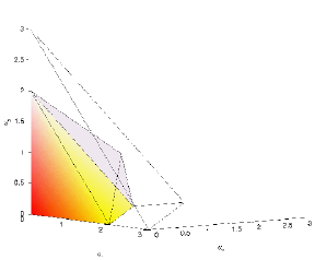
Figure 1: 3 terminals “equidistant” from each of 2 receivers: the original limits capacity to the darker pyramid, while “true” capacity also includes the grayish triangular volume. If the terminals cannot be “heard” by a 3rd receiver, the original greatly overestimates the capacity region by expanding it to the outer pyramid.

It is also significant that the channel gains completely drop out of the condition given by [1]. This fact reduces somewhat the complexity of the condition. Yet some reflection suggests that an admission decision should be influenced by the location of the incumbent and entering terminals. For example, if most active terminals are near a few receivers, then it should make a difference to the system whether a new terminal wants to join the crowded region, or a distant less congested area. Because the original condition is independent of the channel gains, and hence of the terminals’ locations, it cannot adapt to special geographical distributions of the terminals. Thus, the original may yield over-optimistic results under certain channel states, such as when most terminals are in effective range of only a few receivers. For instance, suppose in the previous example that a third receiver exists, but that the terminals are located in such a way that, for each $i$, $h_{i,1}\approx h_{i,2}$ while $h_{i,3}\approx 0$. Thus, $g_{i,1}\approx g_{i,2}\approx 1/2$ and $g_{i,3}\approx 0$. Then, condition (29) still reduces to $\sum_{\begin{subarray}{c}n=1\\ n\neq i\end{subarray}}^{N}\alpha_{n}<2$ for each $i$, and leads to the already discussed capacity region. However, the original condition yields $\sum_{n=1}^{N}\alpha_{n}<3$, which, as illustrated by fig. 1, greatly overestimate the capacity region, by extending it to the outer triangular pyramid with vertexes (0,0,0), (3,0,0), (0,3,0) and (0,0,3)).

Let us now consider the simple asymmetric case of 3 terminals and 2 receivers, with relative gains to the first receiver of 2/3, 1/3, and 1/2, respectively. Condition (29) leads to 3 inequalities per receiver, such as $\frac{2}{3}\alpha_{1}+\frac{1}{3}\alpha_{2}<1$, $\frac{1}{3}\alpha_{1}+\frac{2}{3}\alpha_{2}<1$, $\frac{2}{3}\alpha_{2}+\frac{1}{2}\alpha_{3}<1$, etc. The combination of these inequalities yields a region illustrated by fig. 2(a), which is limited from above by the line segment between (0,0,2) and (1,1,2/3). As already discussed, the result from [1], $\sum_{n=1}^{N}\alpha_{n}<2$, yields a symmetric pyramidal region with vertexes at (0,0,0), (2,0,0), (0,2,0) and (0,0,2) which, as illustrated by fig. 2(b), intersects with — but neither contains nor is contained by — the region described by fig. 2(a).

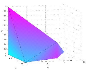
(a) "True" capacity region

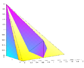
(b) The original formula produces a capacity region that neither includes nor is included by the "true" region

Figure 2: The macro-diversity capacity region for 3 terminals and 2 receivers, for specific asymmetric channel gains

As discussed further in [7], condition (29) yields a low-complexity algorithm for admission-control decisions, which adapts itself in a sensible manner to special channel states. Channel gains also play a prominent role in the feasibility analysis of other multi-cell CDMA systems, such as in [13].

III A class of sub-additive adjustment rules

We focus below on the properties of the individual adjustment function. Thus, from the standpoint of [2], our focus is $I_{i}(\mathbf{p})$, a component of $\mathbf{I}(\mathbf{p})$.

III-A Definition and basic properties

Below, $\Re_{+}^{M}$ denotes the non-negative orthan of $M$-dimensional Euclidean space. $\vec{1}_{M}$ denotes the element of $\Re^{M}$ with each component equal to one (the sub-index may be omitted when appropriate). $\mathbb{N}=\{1,2,\ldots\}$ (the set of Natural numbers).

We study adjustment rules of the general form $f_{i}(\mathbf{p}_{-i})+c_{i}$ where $c_{i}\in\Re_{+}$and $f_{i}$ is quasi-semi-normal.

Definition 1

A function $f:\Re^{M}\rightarrow\Re$ is quasi-semi-normal if it satisfies

$$f(\mathbf{x})\geq 0 \forall\mathbf{x}\in\Re^{M}$$ (1)

$$f(\lambda\vec{1})\leq\lambda f(\vec{1}) \forall\lambda\in(0,1)$$ (2)

$$f(\mathbf{x}+\mathbf{y})\leq f(\mathbf{x})+f(\mathbf{y}) \forall\mathbf{x},\mathbf{y}\in\Re^{M}$$ (3)

$$f(\mathbf{x})\leq f(\left\|\mathbf{x}\right\|_{\infty}\vec{1}_{M}) \forall\mathbf{x}\in\Re^{M}$$ (4)

The preceding conditions are often associated with the words or phrases: non-negativity (1), sub-homogeneity (2), sub-additivity or “the triangle inequality” (3), and monotonicity (4).

Remark 1

Below, we only need our functions to satisfy $f(\lambda\mathbf{x})\leq\lambda f(\mathbf{x})$ at $\mathbf{x}=\vec{1}$. If a function satisfies over its entire domain both (3) and $f(\lambda\mathbf{x})\leq\lambda f(\mathbf{x})$, then it is convex (see also Remark A.1).

Remark 2

Although power vectors are inherently non-negative, the difference between 2 non-negative vectors can, evidently, have negative components. Thus, certain properties in Definition 1 must consider vectors that have negative components.

Remark 3

By Lemma A.1, a function that satisfies condition (3) also satisfies $|f(\mathbf{x})-f(\mathbf{y})|\leq f(\mathbf{x}-\mathbf{y})$ , the “reverse” triangle inequality.

Remark 4

With $\mathbf{x}=\mathbf{y}$ in condition (3) one concludes that $f(2\mathbf{x})\leq 2f(\mathbf{x})$, which easily extends to $f(m\mathbf{x})\leq mf(\mathbf{x})$ for any $m\in\mathbb{N}$.

Remark 5

In (4), the vector $\left\|\mathbf{x}\right\|_{\infty}\vec{1}_{M}$ is obtained from $\mathbf{x}$ by replacing each of its components with the largest of the absolute values of these components, $\left\|\mathbf{x}\right\|_{\infty}$. Thus, $f(\mathbf{x})\leq f(\left\|\mathbf{x}\right\|_{\infty}\vec{1}_{M})$ is a very mild form of monotonicity: “max-monotonicity”.

Remark 6

All semi-norms and norms satisfy conditions (1) , (2) with equality, and (3) (see Definitions A.1 and A.2). All vector (semi-)norms that depend on the absolute value of the components of the vector — such as the sub-family of Hölder norms (Definition A.3) — also satisfy condition (4) (see Theorem A.1).

III-B Some immediate results

Lemma III.1

Suppose that $f:\Re^{M}\rightarrow\Re$ is such that $\lambda\in(0,1)\implies f(\lambda\mathbf{x})\leq\lambda f(\mathbf{x})$, and $f(\mathbf{x}+\mathbf{y})\leq f(\mathbf{x})+f(\mathbf{y})$ then $f$ satisfies $f(r\mathbf{x})\leq rf(\mathbf{x})\quad\forall\mathbf{x}\in\Re^{M}\mbox{ and }r\in\Re_{+}$

Proof:

Consider $m<r<m+1$ for $m\in\mathbb{N}$ (thus, $m$ is the “floor” of $r$, $\lfloor r\rfloor$). Then $f(r\mathbf{x})\equiv f(m\mathbf{x}+(r-m)\mathbf{x})\leq f(m\mathbf{x})+f((r-m)\mathbf{x})$. By Remark 4 $f(m\mathbf{x})\leq mf(\mathbf{x})$. By definition, $r-m\in(0,1)$, $\therefore f((r-m)\mathbf{x})\leq(r-m)f(\mathbf{x})$ by hypothesis. Hence, $f(r\mathbf{x})\leq mf(\mathbf{x})+(r-m)f(\mathbf{x})\equiv rf(\mathbf{x})$

∎

Remark 7

Lemma III.1 is valid for any $\mathbf{x}$, but we only need to apply it at the point $\mathbf{x}=\vec{1}$ (i.e., $f(r\mathbf{x})\leq rf(\mathbf{x})\quad\forall r\in\Re_{+}\mbox{ at }\mathbf{x}=\vec{1}_{M}$).

Lemma III.2

Let $\mathbf{a}\in\Re^{M}$ with $a_{i}\neq 0$. Then the function $f(\mathbf{x}):=\sum_{m=1}^{M}|a_{m}x_{m}|$ for $\mathbf{x}\in\Re^{M}$ satisfies Definition 1.

Proof:

The relevant properties can be checked directly. Alternatively, one may also write $f$ as $f(\mathbf{x})=\|D\mathbf{x}\|_{1}$ where $D$ is the diagonal matrix $D:=\mbox{diag}(a_{1},\cdots,a_{M})$, and $\|\cdot\|_{1}$ denotes the Hölder 1-norm (Definition A.3). Since $D$ is evidently non-singular, Theorem A.3 applies, and $f$ is a norm. ∎

Lemma III.3

For $\mathbf{x}\in\Re^{M}$ and $k=1,\cdots,K$, consider the vectors $\mathbf{a}_{k}=(a_{1,k},\cdots,a_{M,k})$ with $a_{m,k}\neq 0$, and let $y_{k}(\mathbf{x})=\sum_{m=1}^{M}|a_{m,k}x_{m}|$, $\mathbf{y}(\mathbf{x}):=(y_{1}(\mathbf{x}),\cdots,y_{K}(\mathbf{x}))$, and $f(\mathbf{x}):=\|\mathbf{y}(\mathbf{x})\|_{\mu}$, where $\|\cdot\|_{\mu}$ denote a monotonic norm on $\Re^{K}$ (see Definition A.7). Then $f$ satisfies Definition 1 .

Proof:

By Lemma III.2, each $y_{k}$ can be written as $y_{k}(\mathbf{x})=\|\mathbf{x}\|_{\nu_{k}}$where $\|\cdot\|_{\nu_{k}}$ denotes a monotonic norm. Thus, $f$ can be written as $f(\mathbf{x})=\left\|\left[\begin{array}[]{ccc}\|\mathbf{x}\|_{\nu_{1}}&\cdots&\|\mathbf{x}\|_{\nu_{K}}\end{array}\right]^{\prime}\right\|_{\mu}$.

By Theorem A.2 (“norm of norms”), $f(\mathbf{x})$ is a norm. ∎

III-C Some examples

III-C1 The simplest case

Example 1

Consider a single-cell system, and let $h_{j}p_{j}$ denote the received power from terminal $j$. Suppose that each terminal adjusts its power so that $h_{i}p_{i}/(Y_{i}(\mathbf{p}_{-i})+\sigma)=\alpha_{i}$, where $Y_{i}=\sum_{\begin{subarray}{c}n=1\\ n\neq i\end{subarray}}^{N}h_{n}p_{n}$ is the interference affecting terminal $i$, and $\sigma$ represents the average noise power. $p_{i}$ can be written as $f_{i}(\mathbf{p}_{-i})+c_{i}$, with $f_{i}(\mathbf{p}_{-i}):=\sum_{\begin{subarray}{c}n=1\\ n\neq i\end{subarray}}^{N}(\alpha_{i}h_{n}/h_{i})\left|p_{n}\right|$ and $c_{i}=\sigma\alpha_{i}/h_{i}$. By Lemma III.2 , $f_{i}$ is a norm — the absolute value operator has no real effect here — (Definition A.2), and hence has the desired properties (see Remark 6)

III-C2 The macro-diversity scenario

III-C2a System model

Under macro-diversity, the cellular structure is removed and each transmitter is jointly decoded by all receivers[12, 1]. A relevant QoS index for terminal $i$ is the product of its spreading gain by its “carrier to interference ratio” (CIR), $\alpha_{i}$, defined as [1] :

$$\alpha_{i}=\frac{P_{i}h_{i,1}}{Y_{i,1}+\sigma_{1}^{2}}+\cdots+\frac{P_{i}h_{i,K}}{Y_{i,K}+\sigma_{K}^{2}}$$ (5)

where $K$ is the number of receivers in the network, $h_{i,k}$ is the channel gain in the signal from terminal $i$ arriving at receiver $k$, and $Y_{i,k}$ denotes the interfering power experienced by transmitter $i$ at receiver $k$; i.e.,

$$Y_{i,k}:=\sum_{\begin{subarray}{c}n=1\\ n\neq i\end{subarray}}^{N}P_{n}h_{n,k}$$ (6)

Below, we recognise and utilise the vectors:

$$\mathbf{Y}_{i}:=(Y_{i,1},\cdots,Y_{i,K})$$ (7)

$$\boldsymbol{\sigma}:=(\sigma_{1}^{2},\cdots,\sigma_{K}^{2})$$ (8)

III-C2b Normalised adjustment

From (5) one obtains the adjustment process

$$P_{i}=\alpha_{i}\left(\frac{h_{i,1}}{Y_{i,1}+\sigma_{1}^{2}}+\cdots+\frac{h_{i,K}}{Y_{i,K}+\sigma_{K}^{2}}\right)^{-1}$$ (9)

It is unclear that the function on the right side of (9) can be written as $f_{i}(\mathbf{p}_{-i})+c_{i}$ with $c_{i}\in\Re_{+}$and $f_{i}$ satisfying Definition 1. However, an adjustment rule that has the desired form, and over estimates the $P_{i}$ given by (9) can be readily obtained.

Reference [1] simplifies the macro-diversity analysis by including a terminal’s own signal as part of the interference (thus, the sum in equation (6) is taken over all $n$). As an alternative, in equation (9), one can replace each $Y_{i,k}(\mathbf{P})$ with

$$\hat{Y}_{i}:=\max_{k}\{Y_{i,k}\}\equiv\|\mathbf{Y}_{i}\|_{\infty}$$ (10)

and each $\sigma_{k}^{2}$ with

$$\hat{\sigma}:=\max_{k}\{\sigma_{k}^{2}\}\equiv\left\|\boldsymbol{\sigma}\right\|_{\infty}$$ (11)

Then, with

$$h_{i}:=h_{i,1}+\cdots+h_{i,K}$$ (12)

equation (9) becomes

$$P_{i}=\frac{\alpha_{i}}{h_{i}}\left(\hat{Y}_{i}+\hat{\sigma}\right)$$ (13)

Thus, the adjustment process can now be written as $P_{i}=f_{i}(\mathbf{P}_{-i})+c_{i}$ where,

$$f_{i}(\mathbf{P}_{-i}):=\frac{\alpha_{i}}{h_{i}}\left\|\mathbf{Y}_{i}(\mathbf{P}_{-i})\right\|_{\infty}$$ (14)

and

$$c_{i}:=\frac{\alpha_{i}}{h_{i}}\hat{\sigma}$$ (15)

III-C2c Properties of the new macro-diversity adjustment

Proposition III.1

The function $f_{i}$ given by equation (14) satisfies Definition 1.

Proof:

In order to apply Lemma III.3, let $\mathbf{x}:=\mathbf{P}_{-i}$ in such a way that $x_{n}=P_{n}$ for $n<i$ and $x_{n}=P_{n+1}$ for $n\geq i$). Likewise, let $a_{n,k}:=\alpha_{i}h_{n,k}/h_{i}$ for $n<i$ and $a_{n,k}:=\alpha_{i}h_{(n+1),k}/h_{i}$ for $n>i$ . (For example, for $N=3$ and $K=2$, if $i=2$, $x_{1}=P_{1}$, $x_{2}=P_{3}$, $a_{1,k}=\alpha_{2}h_{1,k}/h_{2}$ and $a_{2,k}=\alpha_{2}h_{3,k}/h_{2}$).

The $k$th component of $(\alpha_{i}/h_{i})\mathbf{Y}_{i}(\mathbf{P})$ can then be written as $\sum_{m=1}^{N-1}\left|x_{m}\right|a_{k,m}\equiv\|\mathbf{x}\|_{\nu_{k}}$(see Lemma III.2).

Thus, equation (14) can be written as

$$\left\|\left[\begin{array}[]{ccc}\|\mathbf{x}\|_{\nu_{1}}&\cdots&\|\mathbf{x}\|_{\nu_{K}}\end{array}\right]^{\prime}\right\|_{\infty}$$ (16)

Lemma III.3, with $\|\cdot\|_{\infty}$ playing the role of $\|\cdot\|_{\mu}$, implies that $f_{i}$ is a norm, and has, therefore, the desired properties (see Remark 6). ∎

IV A fixed-point problem

We seek to characterise the conditions leading to the convergence of the process in which each terminal in a wireless communication system, such as the reverse link of a CDMA cell, adjusts its transmission power through a function of the form $f_{i}(\mathbf{p}_{-i})+c_{i}$ with $c_{i}\in\Re_{+}$ and $f_{i}$ satisfying Definition 1.

IV-A Approach

As discussed in subsection II-C, we utilise fixed-point theory, in particular, Theorem B.1, the Banach Contraction Mapping principle.

Remark 8

One can choose any metric to apply Theorem B.1. Below we utilise $d(\mathbf{x},\mathbf{y}):=\left\|\mathbf{x}-\mathbf{y}\right\|_{\infty}$ (see Definition A.4), although the sub-index of $\left\|\cdot\right\|_{\infty}$ is omitted for notational convenience.

IV-B The Banach approach applied to our framework

To apply fixed-point analysis, we need functions defined on $\Re^{N}$ .

Lemma IV.1

For $x\in\Re^{N}$ let $g_{i}(\mathbf{x}):=0\cdot x_{i}+f_{i}(\mathbf{x}_{-i})\equiv f_{i}(\mathbf{x}_{-i})$. If each $f_{i}$ satisfies Definition 1 as a function on $\Re^{N-1}$, then each $g_{i}$ satisfies Definition 1 as a function on $\Re^{N}$.

Proof:

That $g_{i}$ has properties (1) and (4) follows trivially from its definition and the hypothesis.

To verify property (3), the triangle inequality, notice that

$g_{i}(\mathbf{x}+\mathbf{y}):=f_{i}(\mathbf{x}_{-i}+\mathbf{y}_{-i})\leq f_{i}(\mathbf{x}_{-i})+f_{i}(\mathbf{y}_{-i})\equiv g_{i}(\mathbf{x})+g_{i}(\mathbf{y})$

To verify property (2), sub-homogeneity, observe that

$g_{i}(\lambda\mathbf{x}):=f_{i}(\lambda\mathbf{x}_{-i})\leq\lambda f_{i}(\mathbf{x}_{-i})+0\cdot x_{i}\equiv\lambda g_{i}(\mathbf{x})$ ∎

Theorem IV.1

Let $\vec{1}_{M}$ denote the element of $\Re^{M}$ with each component equal to 1. For $\mathbf{x}\in\Re^{N}$ and $i\in\{1,\cdots,N\}$, let the transformation $\mathbf{T}$ be defined by $T_{i}(\mathbf{x}):=f_{i}(\mathbf{x}_{-i})$ where each $f_{i}$ satisfies Definition 1. If $\forall i$, $f_{i}(\vec{1}_{N-1})<1$ then $\mathbf{T}$ is a contraction (Definition B.1).

Proof:

For $x\in\Re^{N}$ let $g_{i}(\mathbf{x}):=0\cdot x_{i}+f_{i}(\mathbf{x}_{-i})\equiv f_{i}(\mathbf{x}_{-i})$. By Lemma IV.1, each $g_{i}$ satisfies Definition 1 as a function on $\Re^{N}$.

Let $\left\|\mathbf{T}(\mathbf{x})-\mathbf{T}(\mathbf{y})\right\|=$

$$\left\|\left[\begin{array}[]{c}g_{1}(\mathbf{x})-g_{1}(\mathbf{y})\\ \vdots\\ g_{N}(\mathbf{x})-g_{N}(\mathbf{y})\end{array}\right]\right\|=\max\left[\begin{array}[]{c}\left|g_{1}(\mathbf{x})-g_{1}(\mathbf{y})\right|\\ \vdots\\ \left|g_{N}(\mathbf{x})-gf(\mathbf{y})\right|\end{array}\right]$$ (17)

By the reverse triangle inequality (see Lemma A.1), $\left|g_{i}(\mathbf{x})-g_{i}(\mathbf{y})\right|\leq g_{i}(\mathbf{x}-\mathbf{y})$. Thus,

$$\max\left[\begin{array}[]{c}\left|g_{1}(\mathbf{x})-g_{1}(\mathbf{y})\right|\\ \vdots\\ \left|g_{N}(\mathbf{x})-g_{N}(\mathbf{y})\right|\end{array}\right]\leq\max\left[\begin{array}[]{c}g_{1}(\mathbf{x}-\mathbf{y})\\ \vdots\\ g_{N}(\mathbf{x}-\mathbf{y})\end{array}\right]$$ (18)

Let $M_{x,y}:=\max(|x_{1}-y_{1}|,\cdots,|x_{N}-y_{N}|)\equiv\left\|\mathbf{x}-\mathbf{y}\right\|$

By monotonicity (condition (4)),

$$g_{i}(\mathbf{x}-\mathbf{y})\leq g_{i}(M_{xy},\cdots,M_{xy})\equiv g_{i}(M_{xy}\vec{1}_{N})$$ (19)

By sub-homogeneity (condition (2))

$$g_{i}(M_{xy}\vec{1})\leq M_{xy}g_{i}(\vec{1})\equiv\left\|\mathbf{x}-\mathbf{y}\right\|g_{i}(\vec{1}_{N})\equiv\left\|\mathbf{x}-\mathbf{y}\right\|f_{i}(\vec{1}_{N-1})$$ (20)

Thus,

$$\left\|\mathbf{T}(\mathbf{x})-\mathbf{T}(\mathbf{y})\right\|\leq\lambda\left\|\mathbf{x}-\mathbf{y}\right\|$$ (21)

where $\lambda:=\max\{f_{1}(\vec{1}_{N-1}),\cdots,f_{N}(\vec{1}_{N-1})\}<1$. ∎

Therefore, with $f_{i}(\vec{1}_{N-1})<1$ for all $i$, the power adjustment transformation is a contraction, and, by Theorem B.1, has a unique fixed point, which can be found by successive approximation. Hence, a feasible power allocation exists that produces all the desired QoS levels. When such allocation fails to exist, a reasonable course of action is to proportionally reduce the QoS parameters [14].

V Capacity implications

Below, we will show how Theorem IV.1 can be applied in the example scenarios of section III-C.

V-A The simplest case

In the scenario of section III-C1, the adjustment rule is $f_{i}(\mathbf{p}_{-i})+c_{i}$, with $f_{i}(\mathbf{p}_{-i}):=\sum_{\begin{subarray}{c}n=1\\ n\neq i\end{subarray}}^{N}(\alpha_{i}h_{n}/h_{i})p_{n}$ and $c_{i}=\sigma\alpha_{i}/h_{i}$.

The channel gains $h_{i}$ can be eliminated by working with the received power levels, $P_{i}:=h_{i}p_{i}$. Now, each terminal adjusts its power so that $P_{i}=\alpha_{i}(Y_{i}(\mathbf{P}_{-i})+\sigma)$ with $Y_{i}=\sum_{\begin{subarray}{c}n=1\\ n\neq i\end{subarray}}^{N}P_{n}$. The adjustment rule can be re-written as $f_{i}(\mathbf{P}_{-i})+c_{i}$, with $f_{i}(\mathbf{P}_{-i}):=\alpha_{i}\sum_{\begin{subarray}{c}n=1\\ n\neq i\end{subarray}}^{N}P_{n}$ and $c_{i}=\sigma\alpha_{i}$.

The feasibility condition of Theorem IV.1 requires that $\alpha_{i}\sum_{\begin{subarray}{c}n=1\\ n\neq i\end{subarray}}^{N}P_{n}<1$ with $P_{n}=1\quad\forall n$ . This leads to the eminently reasonable condition:

$$\alpha_{i}<1/(n-1)$$ (22)

An alternate condition can be obtained through a simple coordinate transformation. Let $q_{i}:=P_{i}/\alpha_{i}$, where $P_{i}$ denotes received power. Under the latest coordinates, the equivalent adjustment is $q_{i}=g_{i}(\mathbf{q}_{-i})+\sigma$ with $g_{i}(\mathbf{q}_{-i}):=\sum_{\begin{subarray}{c}n=1\\ n\neq i\end{subarray}}^{N}q_{n}\alpha_{n}$. Now, the feasibility condition leads to

$$\sum_{\begin{subarray}{c}n=1\\ n\neq i\end{subarray}}^{N}\alpha_{n}<1$$ (23)

Condition (23) is more flexible than, and hence preferable to (22), because if the $\alpha_{i}$’s satisfy (22) they automatically satisfy (23), but not vice-versa.

V-B The macro-diversity scenario

V-B1 Original coordinates

The feasibility condition of Theorem IV.1 when applied to the adjustment rule of section III-C2 leads to (recall that $h_{i}=\sum_{k}h_{i,k}$):

$$\alpha_{i}\sum_{\begin{subarray}{c}n=1\\ n\neq i\end{subarray}}^{N}\frac{h_{n,k}}{h_{i}}<1\quad\forall i,k$$ (24)

V-B2 New coordinates

As with condition (22), condition (26) can be improved upon through a change of coordinates. Equation (13) suggests the change of variable:

$$q_{i}:=\frac{h_{i}P_{i}}{\alpha_{i}}$$ (25)

For convenience, let also

$$g_{i,k}:=\frac{h_{i,k}}{h_{i}}$$ (26)

Now, $P_{n}h_{n,k}\equiv q_{n}\alpha_{n}h_{n,k}/h_{n}\equiv q_{n}\alpha_{n}g_{n,k}$. Corresponding to equation (6), we now have

$$Y_{i,k}:=\sum_{\begin{subarray}{c}n=1\\ n\neq i\end{subarray}}^{N}q_{n}\alpha_{n}g_{n,k}$$ (27)

The adjustment process given by equation (13) can be expressed under the new coordinates, as $q_{i}=g_{i}(\mathbf{q}_{-i})+\hat{\sigma}$ with

$$g_{i}(\mathbf{q}_{-i}):=\max_{k}\sum_{\stackrel{{\scriptstyle n=1}}{{n\neq i}}}^{N}q_{n}\alpha_{n}g_{n,k}\equiv\left\|\mathbf{Y}_{i}(\mathbf{q}_{-i})\right\|_{\infty}$$ (28)

Now, the feasibility condition leads to

$$\max_{i,k}\sum_{\begin{subarray}{c}n=1\\ n\neq i\end{subarray}}^{N}\alpha_{n}g_{nk}<1$$ (29)

VI Non-sub-additive adjustment functions

Below we treat two cases: first the original adjustment rule is (sub)homogeneous for any positive constant, a condition satisfied with equality by all functions considered by [6]. Then, we consider specific models cited as examples by [2]. The discussion in subsection II-D is important to this section.

VI-A (sub)Homogeneous adjustment functions

Let us suppose that the original adjustment function fails to satisfy the triangle inequality, but that, besides non-negative, it is monotonic, and (sub)homogeneous for any positive constant.

Lemma VI.1

Let $f:\Re^{M}\rightarrow\Re$ satisfy (i) non-negativity (1), (ii) monotonicity (4), and (iii) be such that $f(r\mathbf{x})\leq rf(\mathbf{x})\quad\forall\mathbf{x}\in\Re^{M}\mbox{ and }r\in\Re_{+}$. Then there is a function $\phi:\Re^{M}\rightarrow\Re$ such that $f(\mathbf{x})\leq\phi(\mathbf{x})\quad\forall\mathbf{x}\in\Re^{M}$ and $\phi$ satisfies has.

Proof:

By monotonicity, $f(\mathbf{x})\leq f(\left\|\mathbf{x}\right\|_{\infty}\vec{1}_{M})$.

By the sub-homogeneity hypothesis,

$$f(\left\|\mathbf{x}\right\|_{\infty}\vec{1}_{M})\leq\left\|\mathbf{x}\right\|_{\infty}f(\vec{1}_{N})$$ (30)

Thus, $f(\mathbf{x})\leq\left\|\mathbf{x}\right\|_{\infty}f(\vec{1}_{M})$. $\phi$ defined by $\phi(\mathbf{x}):=\left\|\mathbf{x}\right\|_{\infty}f(\vec{1}_{M})$ has the desired properties. ∎

Remark 9

$\phi(\mathbf{x})$ is just a scaled version of the infinity-norm $\left\|\cdot\right\|_{\infty}$ and hence satisfies Definition 1. Thus, if each terminal adjusts its power with a function $f_{i}$ that satisfies non-negativity, monotonicity and (sub)homogeneity, one can analyse the related system in which each terminal adjusts its power with a corresponding $\phi_{i}(\mathbf{x}):=\left\|\mathbf{x}\right\|_{\infty}f_{i}(\vec{1})$.

Remark 10

By Theorem IV.1, if $\phi_{i}(\vec{1})=\left\|\vec{1}\right\|f_{i}(\vec{1})\equiv f_{i}(\vec{1})\leq\lambda_{i}<1$, the $\phi_{i}$-adjustment is asymptotically stable. And since each $f_{i}$ satisfies $f_{i}(\mathbf{x})\leq\phi_{i}(\mathbf{x})$, one can conclude that the “true” adjustment process would behave similarly, if the feasibility condition $f_{i}(\vec{1})\leq\lambda_{i}<1$ is satisfied.

Remark 11

There may exist a different function, $\psi_{i}$, that satisfies Definition 1, and is such that $f_{i}(\mathbf{x})\leq\psi_{i}(\mathbf{x})\leq\phi_{i}(\mathbf{x})$ for all $\mathbf{x}\in\Re^{N-1}$. Indeed, the function we used to “bound” the original macro-diversity adjustment rule has the more exotic “norm of norms” form of eq. (16). Thus, by exploiting the special structure of the original adjustment function, if known, one may obtain a “tighter bound”. Nevertheless, through Lemma VI.1 one can obtain — for a very large family of functions — at least one simple capacity result, when no better such result is available.

Remark 12

Additionally, for $\mathbf{x}\in\Re^{N}$ and $1\leq p<q<\infty$ the Hölder norms satisfy $\left\|\mathbf{x}\right\|_{\infty}\leq\left\|\mathbf{x}\right\|_{q}\leq\left\|\mathbf{x}\right\|_{p}\leq\left\|\mathbf{x}\right\|_{1}$[15, Prop. 9.1.5, p. 345]. This means that if any of these norms is to be used in the process of building a bounding function for the original adjustment rule, it should certainly be $\left\|\cdot\right\|_{\infty}$.

VI-B Yates’ framework

Below, we examine the specific scenarios given by [2] as examples (the notation follows closely [2]).

VI-B1 Scenarios studied in depth

The power adjustment rule for fixed assignment, eq. ([2]-4), can be written as $p_{j}=f_{j}(\mathbf{p})+c_{j}$ with $f_{j}(\mathbf{p})=(\gamma_{j}/h_{a_{j}j})\sum_{i\neq j}h_{a_{j}i}p_{i}$ and $c_{j}=\gamma_{j}\sigma_{a_{j}}/h_{a_{j}j}$. $f_{j}$ is a norm (see Lemma III.2) and hence satisfies Definition 1. Thus, this case perfectly fits our formulation, and in fact is closely related to the simple example discussed in subsection III-C1.

Likewise, the full macro-diversity model has already been fully addressed, and in fact, a corresponding new capacity result been found and discussed (see subsection II-E for a summary).

VI-B2 Other scenarios

The remaining examples of [2] can be easily handled by neglecting random noise. It is straightforward to verify that, if one neglects noise, the corresponding power adjustment rules are homogeneous of degree one, and hence fall under the analysis of subsection VI-A. Below we shall discuss in greater detail the case of multiple-connection (MC) reception. This is an interesting and challenging model which contains another scenario, the minimum power assignment (MPA), as a special case.

VI-B3 The MC scenario

Under MC, user $j$ must maintain an acceptable SIR $\gamma_{j}$ at $d_{j}$ distinct base stations. The system “assigns” $j$ to the $d_{j}$ “best” receivers. Let $Y_{kj}(\mathbf{p}):=\sum_{i\neq j}h_{ki}p_{i}$ and suppose there are $K$ receivers. For $x\in\Re_{+}^{M}$ and $m\leq M$, let $\max(x;m)$ and $\min(x;m)$ denote, respectively, the $m$th largest and the $m$th smallest component of $x$. The requirements of $j$ can be written as $\max\left(\left(p_{j}h_{1j}/(Y_{1j}+\sigma_{1}),\cdots,p_{j}h_{Kj}/(Y_{Kj}+\sigma_{K})\right);d_{j}\right)\geq\gamma_{j}$ or, equivalently, as [2]:

$$p_{j}\geq\gamma_{j}\min\left(\left(\frac{Y_{1j}(\mathbf{p})+\sigma_{1}}{h_{1j}},\cdots,\frac{Y_{Kj}(\mathbf{p})+\sigma_{K}}{h_{Kj}}\right);d_{j}\right)$$ (31)

Under the mild assumption that $\sigma_{k}\ll Y_{kj}$ $\forall k$ and hence can be dropped, the right side of (31) is clearly homogeneous of degree one in $\mathbf{p}$. Hence, the discussion of subsection VI-A applies to this case. Proceeding as in subsection V-B2, we apply condition $f_{j}(\vec{1})<1$ to a slightly different form of (31) in which the variables are $q_{j}=p_{j}/\gamma_{j}$, for which $Y_{kj}(\mathbf{q}):=\sum_{i\neq j}h_{ki}\gamma_{i}q_{i}$. This leads to the condition:

$$\min\left(\left(\sum_{i\neq j}\frac{h_{1i}}{h_{1j}}\gamma_{i},\cdots,\sum_{i\neq j}\frac{h_{Ki}}{h_{Kj}}\gamma_{i}\right);d_{j}\right)<1\,\,\,\forall j$$ (32)

This condition involves weighted sums of $N-1$ quality-of-service parameters where the weights are relative channel gains. For instance, with $d_{j}=3$, condition (32) requires that the 3rd smallest such sum be less than one.

Condition (32) has similarities with (29), its macro-diversity counterpart. But the relative gains are not defined in the same way ($h_{ki}/h_{kj}$ in (32), versus $h_{ki}/\sum_{k}h_{ki}$ in (29)).

In fact, one can apply here the same simplification used for macro-diversity in subsection III-C2. Let $\mathbf{Y}_{j}(\mathbf{p}):=(Y_{1j}(\mathbf{p}),\cdots,Y_{Kj}(\mathbf{p}))$, $\boldsymbol{\sigma}:=(\sigma_{1}^{2},\cdots,\sigma_{K}^{2})$, and $\mathbf{H_{j}}:=(h_{1j},\cdots,h_{Kj})$. Then, replace each $Y_{kj}(\mathbf{p})$ with $\hat{Y}_{j}:=\max_{k}\{Y_{kj}\}\equiv\left\|\mathbf{Y}_{j}\right\|_{\infty}$ and each $\sigma_{k}^{2}$ with $\hat{\sigma}:=\max_{k}\{\sigma_{k}^{2}\}\equiv\left\|\boldsymbol{\sigma}\right\|_{\infty}$. The requirements of user $j$ can now be written as $p_{j}\max(\mathbf{H_{j}};d_{j})/\bigl{(}\hat{Y}_{j}+\hat{\sigma}\bigr{)}\geq\gamma_{j}$, which, with $h_{j}:=\max(\mathbf{H_{j}};d_{j})$, leads to the adjustment $p_{j}h_{j}/\gamma_{j}=\hat{Y}_{j}+\hat{\sigma}$, or equivalently to:

$$q_{j}\equiv\left\|\mathbf{Y}_{j}(\mathbf{q})\right\|_{\infty}+\hat{\sigma}$$ (33)

where $q_{j}:=p_{j}h_{j}/\gamma_{j}$, $Y_{kj}(\mathbf{q})=\sum_{i\neq j}\gamma_{i}q_{i}g_{ki}$ and $g_{ki}:=h_{ki}/h_{i}$.

This leads to the feasibility condition

$$\max_{j,k}\sum_{i\neq j}\gamma_{i}g_{ki}<1$$ (34)

Condition (34) is virtually identical to (29). $g_{ki}:=h_{ki}/h_{i}$ in both cases. However, in (29) $h_{i}:=\sum_{k}h_{ki}$, whereas in (34) $h_{i}:=\max((h_{1i},\cdots,h_{Ki});d_{i})$ (e.g., if $d_{i}=3$, the corresponding $h_{i}$ is the third highest of $i$’s channel gains).

Notice that both conditions (34) and (32) underestimate the capacity of the MC system, but for different reasons. Further work may determine which condition is more advantageous.

Appendix A Norms, metrics and related material

A-A Concepts and definitions

Let $V$ denote a vector space (for a formal definition see [16, pp. 11-12]).

Definition A.1

A function $f\colon V\to\Re$ is called a semi-norm on $V$, if it satisfies:

1. $f(x)\geq 0$ for all $x\in V$

2. $f(\lambda x)=|\lambda|\cdot f(x)$ for all $x\in V$ and all $\lambda\in\Re$ (homogeneity)

3. $f(x+y)\leq f(x)+f(wy)$ for all $x,y\in V$ (the triangle inequality)

Definition A.2

If a semi-norm additionally satisfies $f(x)=0$ if and only if $x=\theta$ (where $\theta$ denotes the zero element of $V$), then $f$ is called a norm on $V$ and $f(x)$ is usually denoted as $\|x\|$.

Remark A.1

It is a simple matter to show that a function that satisfies properties 2 and 3 above is convex. Thus, (semi-)norm-minimisation problems are often well-behaved.

Definition A.3

The Hölder norm with parameter $p\geq 1$ (“$p$-norm”) is denoted as $||\cdot||_{p}$ and defined for $x\in\Re^{N}$ as $\left\|\mathbf{x}\right\|_{p}=(|x_{1}|^{p}+\cdots+|x_{N}|^{p})^{\frac{1}{p}}$.

Remark A.2

With $p=2$, the Hölder norm becomes the familiar Euclidean norm. The $p=1$ case is also often encountered (see Lemma III.2). Furthermore, it can be shown that $\lim_{p\rightarrow\infty}\left\|\mathbf{x}\right\|_{p}=\max(\left|x_{1}\right|,\cdots,\left|x_{N}\right|)$, which leads to the following definition:

Definition A.4

For $x\in\Re^{N}$, the supremum or infinity norm is denoted as $\left\|\cdot\right\|_{\infty}$ and defined as

$$\left\|\mathbf{x}\right\|_{\infty}:=\max(\left|x_{1}\right|,\cdots,\left|x_{N}\right|)$$ (A.1)

Definition A.5

For $\mathbf{x}\in\Re^{N}$ denote as $|\mathbf{x}|$ the vector whose $i$th component is obtained as the absolute value of the $i$th component of $\mathbf{x}$, $|x_{i}|$.

Definition A.6

A norm, $\|\cdot\|$, on $\Re^{N}$ is called an absolute vector norm if it depends only on the absolute values of the components of the vector; that is, for $\mathbf{v}\in\Re^{N}$, and $\mathbf{w}:=|\mathbf{v}|$, $\|\mathbf{v}\|\equiv\|\mathbf{w}\|$.

Definition A.7

For $\mathbf{x}\mbox{ and }\mathbf{y}\in\Re^{N}$, let $\mathbf{x}\leq\mathbf{y}$ mean that $x_{i}\leq y_{i}$ for each $i$. A norm, $\|\cdot\|$, on $\Re^{N}$ is said to be monotonic if, for any $\mathbf{x}\mbox{ and }\mathbf{y}\in\Re^{N}$, $|\mathbf{x}|\leq|\mathbf{y}|$ implies that $\|\mathbf{x}\|\leq\|\mathbf{y}\|$.

Definition A.8

A metric, or distance function is a real valued function $d:X\times X\longrightarrow\Re$ where $X$ is some set, such that, for every $x,y,z\in X$, (i) $d(x,y)\geq 0$, with equality if and only if $x=y$ , (ii) $d(x,y)=d(y,x)$ and (iii) $d(x,z)\leq d(x,y)+d(y,z)$ (the triangle inequality)

Remark A.3

Every norm $\left\|\cdot\right\|$ on a vector space $V$ engenders the metric $d(x,y)=\left\|x-y\right\|$ for $x\,,\,y\,\in V$. A norm generalises the intuitive notion of size or length, while a metric generalises the intuitive notion of distance.

Definition A.9

A metric space $(X,d)$ is a set $X$, together with a metric $d$ defined on $X$. If every Cauchy sequence of points in $X$ has a limit that is also in $X$ then $(X,d)$ is said to be complete.

A-B Useful results from the literature

Lemma A.1

(Reverse triangle inequality) If the function $f\colon V\to\Re$ satisfies the triangle inequality, then $|f(\mathbf{x})-f(\mathbf{y})|\leq f(\mathbf{x}-\mathbf{y})$.

Proof:

Without loss of generality, suppose that $f(\mathbf{x})\geq f(\mathbf{y})$ which implies that $f(\mathbf{x})-f(\mathbf{y})\equiv|f(\mathbf{x})-f(\mathbf{y})|$.

Observe that $\mathbf{x}\equiv(\mathbf{x}-\mathbf{y})+\mathbf{y}$ and apply the triangle inequality to this sum:

Thus, $f(\mathbf{x})\equiv f((\mathbf{x}-\mathbf{y})+\mathbf{y})\leq f(\mathbf{x}-\mathbf{y})+f(\mathbf{y})$ or

$$f(\mathbf{x})-f(\mathbf{y})=|f(\mathbf{x})-f(\mathbf{y})|\leq f(\mathbf{x}-\mathbf{y})$$ (A.2)

∎

Remark A.4

Through (A.2) one can prove that all norms are continuous.

Theorem A.1

A norm on $\Re^{N}$is monotonic if and only if it is an absolute vector norm.

Proof:

See [17] or [15, p.344]. ∎

Theorem A.2

(“Norm of norms”). Let $\|\cdot\|_{\nu_{1}},\cdots,\|\cdot\|_{\nu_{M}}$ be $M$ given vector norms on a real (or complex) vector space $V$, and let $\|\cdot\|_{\mu}$ be a monotonic vector norm on $\Re^{M}$. Then, $\|\mathbf{x}\|:=\left\|\left[\|\cdot\|_{\nu_{1}},\cdots,\|\cdot\|_{\nu_{M}}\right]^{T}\right\|_{\mu}$ is a norm.

Proof:

See [11, Theorem 5.3.1]. ∎

Theorem A.3

Let $\|\cdot\|$ be a monotonic norm on $\Re^{M}$ and let $T$ be an $M\times M$ non-singular real matrix. Then, $\|\mathbf{x}\|_{T}:=\|T\mathbf{x}\|$ for $\mathbf{x}\in\Re^{M}$ defines another monotonic norm on $\Re^{M}$.

Proof:

See [11, Theorem 5.3.2]. ∎

Appendix B Banach fixed-point theory

Definition B.1

A map $T$ from a metric space $(X,d)$ into itself is a contraction if there exists $\lambda\ \in[0,1)$ such that for all $x\mbox{\ ,\ }y\ \in V$, $d(T(x),T(y))\leq\lambda d(x,y)$.

Definition B.2

Picard iterates (Successive approximation): Let $T^{m}(x_{1})$ for $x_{1}\in V$ be defined inductively by $T^{0}(x_{1})=x_{1}$ and $T^{m+1}(x_{1})=T\left(T^{m}(x_{1})\right)$, with $m\in\left\{1,2,\cdots\right\}$.

Theorem B.1

(Banach’ Contraction Mapping Principle) If $T$ is a contraction mapping on a complete metric space $(X,d)$ then there is a unique $x^{*}\in X$ such that $x^{*}=T(x^{*})$. Moreover, $x^{*}$ can be obtained by successive approximation, starting from an arbitrary initial $x_{0}\in X$ ; i.e., for any $x_{0}\in X$, $\lim_{m\rightarrow\infty}T^{m}(x_{0})=x^{*}$.

Proof:

See [18][19, Theorem 3.1.2, p. 74]. ∎

References

- [1] S. V. Hanly, “Capacity and power control in spread spectrum macrodiversity radio networks,” Communications, IEEE Transactions on, vol. 44, no. 2, pp. 247–256, Feb 1996.
- [2] R. D. Yates, “A framework for uplink power control in cellular radio systems,” IEEE Journal on Selected Areas in Communications, vol. 13, no. 7, pp. 1341–1347, Sep. 1995.
- [3] C. W. Sung and W. S. Wong, “A distributed fixed-step power control algorithm with quantization and active link quality protection,” Vehicular Technology, IEEE Transactions on, vol. 48, no. 2, pp. 553–562, Mar 1999.
- [4] K. K. Leung, C. W. Sung, W. S. Wong, and T. Lok, “Convergence theorem for a general class of power-control algorithms,” Communications, IEEE Transactions on, vol. 52, no. 9, pp. 1566–1574, Sept. 2004.
- [5] C. W. Sung and K.-K. Leung, “A generalized framework for distributed power control in wireless networks,” Information Theory, IEEE Transactions on, vol. 51, no. 7, pp. 2625–2635, July 2005.
- [6] M. Schubert and H. Boche, QoS-Based Resource Allocation and Transceiver Optimization, ser. Foundations and Trends in Communications and Information Theory, S. Verdu, Ed. Hanover, MA, USA: Now Publishers Inc., 2005, vol. 2, no. 6.
- [7] V. Rodriguez, R. Mathar, and A. Schmeink, “Capacity and power control in spread spectrum macro-diversity radio networks revisited,” in IEEE Australasian Telecommunications Networking and Application Conference, 2008.
- [8] M. Schubert and H. Boche, “Comparison of -norm and -norm optimization criteria for SIR-balanced multi-user beamforming,” Signal Processing, vol. 84, no. 2, pp. 367–378, 2004.
- [9] V. Rodriguez, R. Mathar, and A. Schmeink, “Generalised multi-receiver radio network: Capacity and asymptotic stability of power control through Banach’s fixed-point theorem,” in Wireless Communications and Networking, IEEE, 2009, to appear.
- [10] V. Rodriguez and R. Mathar, “A generalised multi-receiver radio network and its decomposition into independent transmitter-receiver pairs: Simple feasibility condition and power levels in closed form,” in International Conference on Communications, IEEE, 2009, to appear.
- [11] R. Horn and C. Johnson, Matrix Analysis. Cambridge, UK: Cambridge University Press, 1985.
- [12] S. V. Hanly, “Information capacity of radio networks,” Ph.D. dissertation, Univ. of Cambridge, 1993.
- [13] D. Catrein, L. A. Imhof, and R. Mathar, “Power control, capacity, and duality of uplink and downlink in cellular CDMA systems,” IEEE Transactions on Communications, vol. 52, no. 10, pp. 1777–1785, Oct. 2004.
- [14] R. Mathar and A. Schmeink, “Proportional QoS adjustment for achieving feasible power allocation in CDMA systems,” Communications, IEEE Transactions on, vol. 56, no. 2, pp. 254–259, February 2008.
- [15] D. S. Bernstein, Matrix Mathematics: Theory, Facts, and Formulas with Application to Linear Systems Theory. Princeton University Press, 2005.
- [16] D. G. Luenberger, Optimization by vector space methods. New York: Wiley-Interscience, 1969.
- [17] F. Bauer, J. Stoer, and C. Witzgall, “Absolute and monotonic norms,” Numerische Mathematik, vol. 3, no. 1, pp. 257–264, 1961.
- [18] S. Banach, “Sur les opérations dans les ensembles abstraits et leur application aux équations intégrales,” Ph.D. dissertation, University of Lwów, Poland (now Ukraine), 1920, published: Fundamenta Mathematicae 3, 1922, pages 133-181.
- [19] V. I. Istrăţescu, Fixed point theory : an introduction. Dordrecht, Holland: Reidel Publishing Company, 1981.