$B_{s1}(5830)$ and $B_{s2}^{*}(5840)$

Abstract

In this paper we investigate the strong decays of the two newly observed bottom-strange mesons $B_{s1}(5830)$ and $B_{s2}^{*}(5840)$ in the framework of the quark pair creation model. The two-body strong decay widths of $B_{s1}(5830)^{0}\to B^{*+}K^{-}$ and $B_{s2}^{*}(5840)^{0}\to B^{+}K^{-},\,B^{*+}K^{-}$ are calculated by considering $B_{s1}(5830)$ to be a mixture between $|^{1}P_{1}\rangle$ and $|^{3}P_{1}\rangle$ states, and $B_{s2}^{*}(5840)$ to be a $|^{3}P_{2}\rangle$ state. The double pion decay of $B_{s1}(5830)$ and $B_{s2}^{*}(5840)$ is supposed to occur via the intermediate state $\sigma$ and $f_{0}(980)$. Although the double pion decay widths of $B_{s1}(5830)$ and $B_{s2}^{*}(5840)$ are smaller than the two-body strong decay widths of $B_{s1}(5830)$ and $B_{s2}^{*}(5840)$, one suggests future experiments to search the double pion decays of $B_{s1}(5830)$ and $B_{s2}^{*}(5840)$ due to their sizable decay widths.

I Introduction

Heavy flavor physics is an interesting research field. In the past three years, a series of the new observations of the heavy flavor hadrons, such as $D_{sJ}(2317)$, $D_{sJ}(2460)$ Aubert:2003fg ; Krokovny:2003zq ; Besson:2003cp ; others , $D_{sJ}(2860)$ 2860-babar , $D_{sJ}(2715)$ belle-2715 ; Belle-2715 , $\Lambda_{c}(2880,2940)^{+}$, $\Xi_{c}(2980,3077)^{+,0}$, $\Omega_{c}(2768)^{0}$ babar-2880 ; belle-2880 ; babar-2980-3077 ; belle-2980-3077 ; new-Xi3055 ; babar-omega ; cleo-2880 , $\Sigma_{b}^{\pm}$, $\Sigma_{b}^{*\pm}$ CDF ; CDF-1 , and $\Xi_{b}$ D0-Xi ; CDF-Xi ; CDF-Xi-1 , have made the study of heavy flavor physics active and attractive.

Up to now, there only exist two established bottom-strange mesons in Particle Data Group (PDG) PDG . However, recent observations of the two orbitally excited $B_{s}$ mesons announced by CDF CDF-Bs ; D0-Bs and D0 experiments make the bottom-strange mass spectrum become abundant. The CDF collaboration reported $m_{B_{s1}}=5829.4\pm 0.7$ MeV and $m_{B_{s2}^{*}}=5839.6\pm 0.7$ MeV CDF-Bs . The D0 collaboration confirmed $B_{s2}^{*}(5840)$ state with $m_{B_{s2}^{*}}=5839.6\pm 1.1(\mathrm{stat}.)\pm 0.7(\mathrm{syst}.)$ MeV D0-Bs , and indicated that $B_{s1}(5830)$ was not observed with the available data set D0-Bs . In Fig. 1, one lists all bottom-strange mesons observed by the experiments.

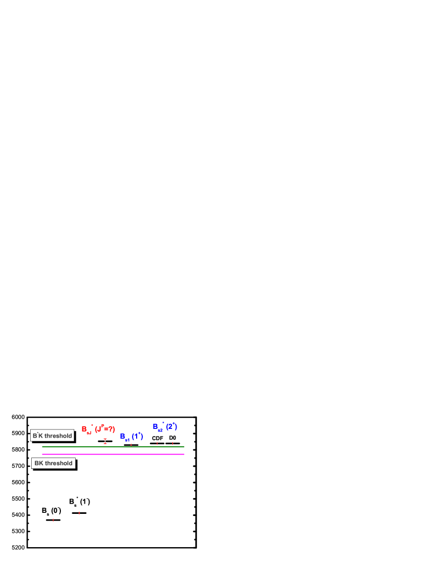
Figure 1: The mass spectrum of bottom-strange mesons. The data is taken from particle date group (PDG) PDG and the CDF and D0 experiments CDF-Bs ; D0-Bs .

For heavy-light meson system, we can group it into several doublets in terms of the heavy quark effective theory (HQET), i.e. $j_{\ell}^{P}=\frac{1}{2}^{-}$ $H$ doublet $(0^{-},1^{-})$ with orbital angular momentum $L=0$, $j_{\ell}^{P}=\frac{1}{2}^{+}$ $S$ doublet $(0^{+},1^{+})$ and $j_{\ell}^{P}=\frac{3}{2}^{+}$ $T$ doublet $(1^{+},2^{+})$ with $L=1$. The D0 and CDF experiments indicated that $B_{s1}(5830)$ and $B_{s2}^{*}(5840)$ correspond to the states respectively with $J^{P}=1^{+}$ and $J^{P}=2^{+}$ in $T$ doublet CDF-Bs ; D0-Bs .

Before finding $B_{s1}(5830)$ and $B_{s2}^{*}(5840)$, many theoretical groups were involved in the study of the properties of heavy-light mesons. In Ref. godfrey , the authors studied the masses of P-wave states by the relativistic quark model, then calculated their decay widths using both the pseudoscalar emission model and the flux-tube-breaking model. Eichten, Hill and Quigg estimated the masses and the decay widths of orbitally excited heavy-light mesons by using the heavy quark symmetry, which is supplemented by the insights from the potential model EHQ . Ebert, Galkin and Faustov calculated the mass spectrum of the orbitally excited heavy-light mesons according to the relativistic quark model EGF . Then Di Pierro and Eichten carried out a detailed study of the orbital and radial excited heavy mesons DE . By the effective Lagrangian constructed in the chiral symmetry and the heavy quark limit, Falk and Mehen examined the decays of the excited heavy mesons including the leading power corrections to the heavy quark limit FM . In the approach of Lattic QCD, the authors of Ref. Green obtained the mass spectrum of the excited heavy-light meson. In Ref. colangelo , Colangelo, Fazio and Ferrandes studied the structures and the decays of the orbitally excited states. Matsuki, Morii and Sudoh obtained the mass spectrum of the heavy-light systems by the semi-relativistic quark model Matsuki . According to the chiral quark model, Zhong and Zhao performed the calculations of the strong decays of the heavy-light mesons zhong . All of the above mentioned work refers to the bottom-strange mesons.

The observations of the two bottom-strange states have inspired our interest in $B_{s1}(5830)$ and $B_{s2}^{*}(5840)$, especially in their decay properties. In Ref. semi-liu , one performed the calculations of the semileptonic decays of $B_{s1}(5830)$ and $B_{s2}^{*}(5840)$. At present, the CDF and D0 experiments only carried out the measurements of the masses of $B_{s1}(5830)$ and $B_{s2}^{*}(5840)$. However, the total widths of $B_{s1}(5830)$ and $B_{s2}^{*}(5840)$ are still missing. Thus the study on their strong decay becomes an interesting and important topic, which will be helpful not only for obtaining the information of the total widths of $B_{s1}(5830)$ and $B_{s2}^{*}(5840)$, but also for testing the model applied to the calculation of the strong decay of $B_{s1}(5830)$ and $B_{s2}^{*}(5840)$. In this work, we focus on the calculation of the strong decay rates of $B_{s1}(5830)$ and $B_{s2}^{*}(5840)$ using the ${}^{3}P_{0}$ model.

This work is organized as follows. After the introduction, we briefly review the ${}^{3}P_{0}$ model. In Sec. III and Sec. IV, we present the formulation and the numerical result of the two-body and double pion decays of $B_{s1}(5830)$ and $B_{s2}^{*}(5840)$, respectively. The last section is a short summary.

II A review of the ${}^{3}P_{0}$ model

In this work we use the ${}^{3}P_{0}$ model Micu ; yaouanc ; yaouanc-1 ; yaouanc-book ; Beveren ; BSG ; sb , also known as the Quark Pair Creation (QPC) model, to calculate the strong decays of $B_{s1}(5830)$ and $B_{s2}^{*}(5840)$. This model is applicable to Okubo-Zweig-Iizuka (OZI) allowed strong decays of a hadron into two other hadrons, which are expected to be the dominant decay modes of a meson if they are allowed. The ${}^{3}P_{0}$ model has been widely used since it is successful when applied extensively to the calculation of the strong decay of hadron qpc-1 ; qpc-2 ; qpc-90 ; ackleh ; Zou ; liu ; Close:2005se ; lujie ; xiangliu-2860 ; xiangliu-heavy ; Li:2008mz .

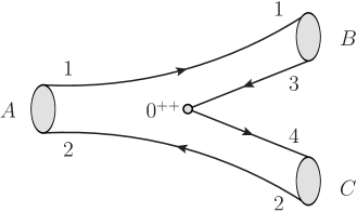
Figure 2: The ${}^{3}P_{0}$ decay mechanism for meson decay $A\to B+C$.

In the QPC model, the heavy meson decay occurs via a quark-antiquark pair production from the vacuum, which is depicted in Fig. 2. The created quark pair is of the quantum number of the vacuum, $0^{++}$ Micu ; yaouanc . In the non-relativistic limit, the transition operator is expressed as

$$T = -3\gamma\sum_{m}\>\langle 1\;m;1\;-m|0\;0\rangle\,\int\!{\rm d}{\textbf{k}}_{3}\;{\rm d}{\textbf{k}}_{4}\delta^{3}({\textbf{k}}_{3}+{\textbf{k}}_{4}){\cal Y}_{1m}\left(\frac{{\textbf{k}}_{3}-{\textbf{k}_{4}}}{2}\right)\;$$ (1)

$$\times\chi^{34}_{1,-\!m}\;\varphi^{34}_{0}\;\,\omega^{34}_{0}\;d^{\dagger}_{3i}({\textbf{k}}_{3})\;b^{\dagger}_{4j}({\textbf{k}}_{4})\,,$$

where $i$ and $j$ are the SU(3)-color indices of the created quark and anti-quark. $\varphi^{34}_{0}=(u\bar{u}+d\bar{d}+s\bar{s})/\sqrt{3}$ and $\omega_{0}^{34}=\delta_{ij}$ are for flavor and color singlets, respectively. $\chi_{{1,-m}}^{34}$ is a triplet state of spin. $\mathcal{Y}_{\ell m}(\mathbf{k})\equiv|\mathbf{k}|^{\ell}Y_{\ell m}(\theta_{k},\phi_{k})$ is the $\ell$th solid harmonic polynomial. $\gamma$ is a dimensionless constant which denotes the strength of quark pair creation from vacuum and can be extracted by fitting data. We adopt the mock state to describe the meson with the spatial wave function $\Psi_{n_{A}L_{A}M_{L_{A}}}\left(\mathbf{k}_{1},\mathbf{k}_{2}\right)$ in the momentum representation mockmeson

$$\left|A(n_{A}\mbox{}^{2S_{A}+1}L_{A}\,\mbox{}_{J_{A}M_{J_{A}}})({\textbf{K}}_{A})\right\rangle$$

$$=\sqrt{2E_{A}}\sum_{M_{L_{A}},M_{S_{A}}}\left\langle L_{A}M_{L_{A}}S_{A}M_{S_{A}}|J_{A}M_{J_{A}}\right\rangle$$

$$\quad\times\int\rm d\mathbf{k}_{1}\rm d\mathbf{k}_{2}\delta^{3}\left(\textbf{K}_{A}-\mathbf{k}_{1}-{\mathbf{k}}_{2}\right)\Psi_{n_{A}L_{A}M_{L_{A}}}\left(\mathbf{k}_{1},\mathbf{k}_{2}\right)$$

$$\quad\times\chi^{12}_{S_{A}M_{S_{A}}}\varphi^{12}_{A}\omega^{12}_{A}\left|\;q_{1}\left(\mathbf{k}_{1}\right)\bar{q}_{2}\left(\mathbf{k}_{2}\right)\right\rangle,$$ (2)

which satisfies the normalization conditions

$$\langle A(\textbf{K}_{A})|A(\textbf{K}^{\prime}_{A})\rangle = 2E_{A}\,\,\delta^{3}(\textbf{K}_{A}-\textbf{K}^{\prime}_{A}),\;$$ (3)

$$\langle q_{i}(\mathbf{k}_{i})|q_{j}(\mathbf{k}_{j})\rangle = \delta_{ij}\delta^{3}(\mathbf{k}_{i}-\mathbf{k}_{j}),\;$$ (4)

$$\langle\bar{q}_{i}(\mathbf{k}_{i})|\bar{q}_{j}(\mathbf{k}_{j})\rangle = \delta_{ij}\delta^{3}(\mathbf{k}_{i}-\mathbf{k}_{j}),\;$$ (5)

$$\int\rm d\mathbf{k}_{1}\rm d\mathbf{k}_{2}\delta^{3}(\textbf{K}_{A}-\mathbf{k}_{1}-\mathbf{k}_{2})\Psi_{A}(\mathbf{k}_{1},\mathbf{k}_{2})\Psi_{A^{\prime}}(\mathbf{k}_{1},\mathbf{k}_{2})=\delta_{A^{\prime}A}.$$ (6)

The subscripts 1 and 2 in (II) refer to the quark and the anti-quark within the meson $A$, respectively. ${\textbf{K}}_{A}$ is the momentum of the meson $A$. $\mathbf{S}_{A}=\mathbf{s}_{q_{1}}+\mathbf{s}_{q_{2}}$ is the total spin. $\mathbf{J}_{A}=\mathbf{L}_{A}+\mathbf{S}_{A}$ denotes the total angular momentum.

For $A\to B+C$ process, the S-matrix is depicted as

$$\langle BC|S|A\rangle=I-i2\pi\delta(E_{f}-E_{i})\langle{}BC|T|A\rangle.$$ (7)

In the center of the mass frame of the meson $A$, $\textbf{K}_{A}=0$ and $\textbf{K}_{B}=-\textbf{K}_{C}=\textbf{K}$. Then, we have

$$\langle BC|T|A\rangle=\sqrt{8E_{A}E_{B}E_{C}}\;\;\gamma\!\!\!\!\!\!\!\!\!\!\!\sum_{\begin{array}[t]{l}\scriptstyle M_{L_{A}},M_{S_{A}},\\ \scriptstyle M_{L_{B}},M_{S_{B}},\\ \scriptstyle M_{L_{C}},M_{S_{C}},m\end{array}}\!\!\!\!\!\!\!\!\langle 1\;m;1\;-m|\;0\;0\rangle$$ (11)

$$\quad\times\langle L_{A}M_{L_{A}}S_{A}M_{S_{A}}|J_{A}M_{J_{A}}\rangle\langle L_{B}M_{L_{B}}S_{B}M_{S_{B}}|J_{B}M_{J_{B}}\rangle$$

$$\quad\times\langle L_{C}M_{L_{C}}S_{C}M_{S_{C}}|J_{C}M_{J_{C}}\rangle\langle\varphi^{13}_{B}\varphi^{24}_{C}|\varphi^{12}_{A}\varphi^{34}_{0}\rangle$$

$$\quad\times\langle\chi^{13}_{S_{B}M_{S_{B}}}\chi^{24}_{S_{C}M_{S_{C}}}|\chi^{12}_{S_{A}M_{S_{A}}}\chi^{34}_{1-\!m}\rangle I^{M_{L_{A}},m}_{M_{L_{B}},M_{L_{C}}}({\textbf{K}})\;.$$

The spatial integral $I^{M_{L_{A}},m}_{M_{L_{B}},M_{L_{C}}}(\textbf{K})$ reads as

$$I^{M_{L_{A}},m}_{M_{L_{B}},M_{L_{C}}}(\textbf{K})=\int\!\rm d\mathbf{k}_{1}\rm d\mathbf{k}_{2}\rm d\mathbf{k}_{3}\rm d\mathbf{k}_{4}\,\delta^{3}(\mathbf{k}_{1}+\mathbf{k}_{2})$$

$$\quad\times\delta^{3}(\mathbf{k}_{3}+\mathbf{k}_{4})\delta^{2}(\textbf{K}_{B}-\mathbf{k}_{1}-\mathbf{k}_{3})\delta^{3}(\textbf{K}_{C}-\mathbf{k}_{2}-\mathbf{k}_{4})$$

$$\quad\times\Psi^{*}_{n_{B}L_{B}M_{L_{B}}}(\mathbf{k}_{1},\mathbf{k}_{3})\Psi^{*}_{n_{C}L_{C}M_{L_{C}}}(\mathbf{k}_{2},\mathbf{k}_{4})$$

$$\quad\times\Psi_{n_{A}L_{A}M_{L_{A}}}(\mathbf{k}_{1},\mathbf{k}_{2})\mathcal{Y}_{1m}\Big{(}\frac{\mathbf{k}_{3}-\mathbf{k}_{4}}{2}\Big{)}.$$ (13)

The rest of the model is just to describe the overlap of the initial meson ($A$) and the created pair with the two final mesons ($B$ and $C$), and then finally to calculate the probability that the rearrangement will occur. The radial portions of the meson space wavefunction can be expressed in certain functional forms, which encompass the simple harmonic oscillator (HO) wavefunction

$$\Psi_{nLM}(\mathbf{k})=\mathcal{N}_{nL}\exp\left(-\frac{R^{2}\mathbf{k}^{2}}{2}\right)\mathcal{Y}_{LM}(\mathbf{k})\,\mathcal{P}(\mathbf{k}^{2}),$$ (14)

where $\mathcal{P}(\mathbf{k}^{2})$ is the polynomial of $\mathbf{k}^{2}$. $\mathbf{k}$ is the relative momentum between the quark and the anti-quark within a meson. For example, meson $A$ is composed of quark $1$ and anti-quark $2$, so, $\mathbf{k}_{A}=(m_{2}\mathbf{k}_{1}-m_{1}\mathbf{k}_{2})/(m_{1}+m_{2}).$ $\mathcal{N}_{nL}$ denotes the normalization coefficient. In this work, for the decay channels of interest, what we need is only the lowest two states without the radical excitation, i.e.

$$\Psi_{00}(\mathbf{k}) = \frac{1}{\pi^{3/4}}R^{3/2}\exp\left(-\frac{R^{2}\mathbf{k}^{2}}{2}\right),$$ (15)

$$\Psi_{1\mu}(\mathbf{k}) = i\frac{\sqrt{2}}{\pi^{3/4}}R^{5/2}k_{\mu}\exp\left(-\frac{R^{2}\mathbf{k}^{2}}{2}\right),$$ (16)

where $k_{\mu}$ is the spherical component of the vector $\mathbf{k}$, which is defined as $k_{\pm 1}=\mp(k_{x}\pm{}ik_{y})/\sqrt{2}$ and $k_{0}=k_{z}$.

In terms of Wigner’s $9j$ symbol, the spin matrix element can be written as yaouanc-book

$${\langle\chi^{13}_{B_{C}M_{B_{C}}}\chi^{24}_{S_{C}M_{S_{C}}}|\chi^{12}_{S_{A}M_{S_{A}}}\chi^{34}_{1-\!m}\rangle}$$

$$=(-1)^{S_{C}+1}\Big{[}3(2S_{B}+1)(2S_{C}+1)(2S_{A}+1)\Big{]}^{1/2}$$ (19)

$$\quad\times\sum_{S,M_{s}}\langle S_{B}M_{S_{B}}S_{C}M_{S_{C}}|SM_{s}\rangle$$

$$\quad\times\langle SM_{s}|S_{A}M_{S_{A}};1,-m\rangle\;\left\{\begin{array}[]{ccc}1\over 2&1\over 2&S_{B}\\ 1\over 2&1\over 2&S_{C}\\ S_{A}&1&S\end{array}\right\}\;.$$

With the transition amplitude obtained in (11), the helicity amplitude $\mathcal{M}^{M_{J_{A}}M_{J_{B}}M_{J_{C}}}$ can be extracted from

$$\langle{}BC|T|A\rangle=\delta^{3}(\mathbf{K}_{B}+\mathbf{K}_{C}-\mathbf{K}_{A})\mathcal{M}^{M_{J_{A}}M_{J_{B}}M_{J_{C}}}.$$ (20)

The decay width for the process $A\to BC$ in terms of the helicity amplitude is

$$\Gamma=\pi^{2}\frac{|\mathbf{K}|^{2}}{M_{A}^{2}}\frac{1}{2J_{A}+1}\sum_{\begin{array}[t]{l}\scriptstyle M_{J_{M_{A}}},M_{J_{M_{B}}},\\ \scriptstyle\quad M_{J_{M_{C}}}\end{array}}\Big{|}\mathcal{M}^{M_{J_{A}}M_{J_{B}}M_{J_{C}}}\Big{|}^{2}\,.$$

For the sake of convenience, one usually works out the partial wave amplitude first via the Jacob-Wick formula convert

$${\mathcal{M}}^{JL}(A\rightarrow BC)=\frac{\sqrt{2L+1}}{2J_{A}+1}\!\!\sum_{M_{J_{B}},M_{J_{C}}}\langle L0JM_{J_{A}}|J_{A}M_{J_{A}}\rangle$$

$$\quad\quad\quad\times\langle J_{B}M_{J_{B}}J_{C}M_{J_{C}}|JM_{J_{A}}\rangle\mathcal{M}^{M_{J_{A}}M_{J_{B}}M_{J_{C}}}({\textbf{K}}),$$ (22)

where $\mathbf{J}=\mathbf{J}_{B}+\mathbf{J}_{C}$ and $\mathbf{J}_{A}=\mathbf{J}_{B}+\mathbf{J}_{C}+\mathbf{L}$. Then one calculates the decay width in terms of the partial wave amplitude

$$\Gamma=\pi^{2}\frac{{|\textbf{K}|}}{M_{A}^{2}}\sum_{JL}\Big{|}\mathcal{M}^{JL}\Big{|}^{2},$$ (23)

where $|\textbf{K}|$, as mentioned above, is the three momentum of the daughter mesons in the parent’s center of mass frame.

III Two-body strong decays

The two-body strong decays of $B_{s1}(5830)^{0}$ and $B_{s2}^{*}(5840)^{0}$ allowed by the phase space include

$$\left\{\begin{array}[]{l}B_{s1}(5830)^{0}\to B^{*+}K^{-},\;B^{*0}\bar{K}^{0}\\ B_{s2}^{*}(5840)^{0}\to B^{+}K^{-},\;B^{0}\bar{K}^{0}\\ B_{s2}^{*}(5840)^{0}\to B^{*+}K^{-},\;B^{*0}\bar{K}^{0}\end{array}\right.\,.$$

Due to the conservations of the angular momentum and the parity, the $B\bar{K}$ decay mode for $B_{s1}(5830)^{0}$ is forbidden.

Before entering the calculation, we firstly introduce the component of $B_{s1}(5830)^{0}$ with $J^{P}=1^{+}$. In quark model, $B_{s1}(5830)^{0}$ is usually considered as the mixture of the two basis states $|^{1}P_{1}\rangle$ and $|^{3}P_{1}\rangle$ godfrey

$$\left(\begin{array}[]{c}\left|1^{+},j_{l}^{P}=\frac{1}{2}^{+}\right\rangle\\ \left|1^{+},j_{l}^{P}=\frac{3}{2}^{+}\right\rangle\end{array}\right)=\left(\begin{array}[]{cc}\cos\theta&\sin\theta\\ -\sin\theta&\cos\theta\end{array}\right)\left(\begin{array}[]{c}\left|{}^{1}P_{1}\right\rangle\\ \left|{}^{3}P_{1}\right\rangle\end{array}\right)\,,$$ (29)

where $\theta$ is the mixing angle with $\theta=-\tan^{-1}\sqrt{2}=-54.7^{\circ}$ based on the estimate in the heavy quark limit. However, one can not determine the exact value of $\theta$ when $m_{Q}$ is finite. In Ref. zhu-dai , Dai and Zhu indicated that there does not exist a large difference between the value of $\theta$ for the case of $m_{Q}\to finity$ and that for the case of $m_{Q}\to\infty$.

By the ${}^{3}P_{0}$ model, we obtain a general relationship between S-wave (D-wave) decay amplitude of $s\bar{b}(^{1}P_{1})\to B^{*}\bar{K}$ and that of $s\bar{b}(^{3}P_{1})\to B^{*}\bar{K}$

$$\left(\begin{array}[]{c}\mathcal{M}\left[|s\bar{b}(^{1}P_{1})\rangle\to|B^{*}\bar{K}\rangle_{S-wave}\right]\\ \\ \mathcal{M}\left[|s\bar{b}(^{1}P_{1})\rangle\to|B^{*}\bar{K}\rangle_{D-wave}\right]\end{array}\right)$$ (33)

$$\quad\quad\quad=\left(\begin{array}[]{cc}-\frac{1}{\sqrt{2}}&0\\ \\ 0&\sqrt{2}\end{array}\right)\left(\begin{array}[]{c}\mathcal{M}\left[|s\bar{b}(^{3}P_{1})\rangle\to|B^{*}\bar{K}\rangle_{S-wave}\right]\\ \\ \mathcal{M}\left[|s\bar{b}(^{3}P_{1})\rangle\to|B^{*}\bar{K}\rangle_{D-wave}\right]\end{array}\right)\,.$$ (40)

Further the amplitude squared of $1^{+}\to B^{*}\bar{K}$ decay can be expressed as

$$\left\{\begin{array}[]{l}|M[1^{+}(S)\to(B^{*}\bar{K})_{S-wave}]|^{2}\\ |M[1^{+}(S)\to(B^{*}\bar{K})_{D-wave}]|^{2}\\ |M[1^{+}(T)\to(B^{*}\bar{K})_{S-wave}]|^{2}\\ |M[1^{+}(T)\to(B^{*}\bar{K})_{D-wave}]|^{2}\end{array}\right.\propto\left\{\begin{array}[]{l}(\cos\theta-{\sqrt{2}}\sin\theta)^{2}|A_{S}|^{2}\\ (\cos\theta+\frac{1}{\sqrt{2}}\sin\theta)^{2}|A_{D}|^{2}\\ (-\sin\theta-{\sqrt{2}}\cos\theta)^{2}|A_{S}|^{2}\\ (-\sin\theta+\frac{1}{\sqrt{2}}\cos\theta)^{2}|A_{D}|^{2}\end{array}\right.$$ (49)

with $A_{S(D)}=\mathcal{M}\left[|s\bar{b}(^{1}P_{1})\rangle\to|B^{*}\bar{K}\rangle_{S(D)-wave}\right]$.

In Fig. 3, one shows the variation of the factor in front of $|A_{S(D)}|^{2}$ of Eq. (49) to the mixing angle $\theta$. For the case of the decay of $1^{+}$ state in $S$ doublet, $1^{+}$ state mainly decays into $B^{*}\bar{K}$ by the S-wave amplitude since there exists the constructive (destructive) interference between the S-wave (D-wave) decay amplitudes of $|^{1}P_{1}\rangle$ and $|^{3}P_{1}\rangle$ states when taking $\theta=-54.7^{\circ}$. On the contrary, for the case of $1^{+}$ state in $T$ doublet, the D-wave decay amplitude play the dominant role for the decay of $1^{+}$ state into $B^{*}\bar{K}$ since the effect of the interference between the S-wave (D-wave) decay amplitudes of $|^{1}P_{1}\rangle$ and $|^{3}P_{1}\rangle$ states is contrary to that of $1^{+}$ state in $S$ doublet when taking $\theta=-54.7^{\circ}$. This is the reason for the total widths of $1^{+}$ states existing in $S$ and $T$ doublets being wide and narrow respectively.

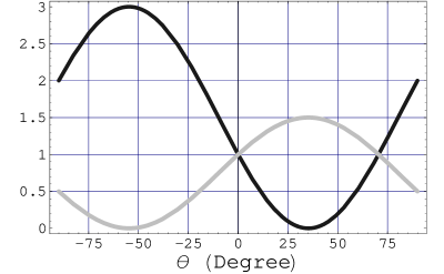
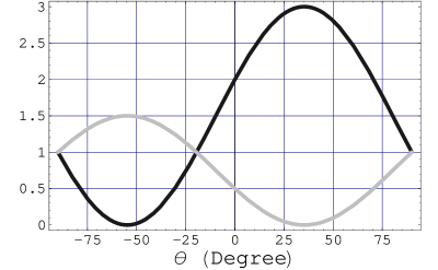
(a)	(b)

Figure 3: The dependence of the factor in front of $|A_{S,D}|^{2}$ of Eq. (49) on $\theta$. The black and grey lines in both of the diagrams correspond to S-wave and D-wave decays, respectively. Here diagrams (a) and (b) are the results of $1^{+}$ states in $S$ and $T$ doublets, respectively.

Mode	$(J,L)$	Decay amplitude
$B_{s1}(5830)^{0}\to$	(1,0)	$\frac{\sqrt{2}(-\sin\theta-\sqrt{2}\cos\theta)\gamma\sqrt{E_{A}E_{B}E_{C}}}{9}[I_{0}-2I_{\pm}]$
$B^{*+}K^{-}$	(1,2)	$\frac{-{2}(-\sin\theta+1/\sqrt{2}\cos\theta)\gamma\sqrt{E_{A}E_{B}E_{C}}}{9}[I_{0}+I_{\pm}]$
$B_{s2}^{*}(5840)^{0}\to$
$B^{+}K^{-}$	(0,2)	$\frac{-{2}}{3\sqrt{15}}\gamma\sqrt{E_{A}E_{B}E_{C}}[I_{0}+I_{\pm}]$
$B_{s2}^{*}(5840)^{0}\to$
$B^{*+}K^{-}$	(1,2)	$\frac{-\sqrt{2}}{3\sqrt{5}}\gamma\sqrt{E_{A}E_{B}E_{C}}[I_{0}+I_{\pm}]$

Table 1: The decay amplitude of the two-body strong decays of $B_{s1}(5830)^{0}$ and $B^{*}_{s2}(5840)^{0}$. Here functions $I_{\pm,0}$ are listed in the appendix.

In Table 1, one presents the two-body decay amplitudes of $B_{s1}(5830)^{0}$ and $B_{s2}^{*}(5840)^{0}$ calculated by the ${}^{3}P_{0}$ model. The values of the parameters involved in the ${}^{3}P_{0}$ model include the strength of the quark pair creation from the vacuum and the $R$ value in the HO wave function listed in Table 2. As a dimensionless parameter in the ${}^{3}P_{0}$ model, $\gamma$ is taken as $6.9$ Godfrey , which is $\sqrt{96\pi}$ times larger than that used by the other groups close-3p0 ; kokoski . The $R$ value in the HO wave function can be fixed to reproduce the realistic root mean square (RMS) radius by solving the schrödinger equation with the linear potential godfrey .

	mass (MeV) PDG	$R$ (GeV-1) godfrey
$B_{s1}(5830)$	5829.4	1.79
$B_{s2}^{*}(5840)$	5839.7	1.92
$B$	5279.2	1.59
$B^{*}$	5325.1	1.75
$B_{s}$	5336.3	1.45
$B_{s}^{*}$	5412.8	1.59
$K$	493.7	1.41
$f_{0}(980)$	980.0	2.00

Table 2: The parameters relevant to the two-body strong decays of $B_{s1}(5830)^{0}$ and $B^{*}_{s2}(5840)^{0}$ in the ${}^{3}P_{0}$ model PDG ; godfrey .

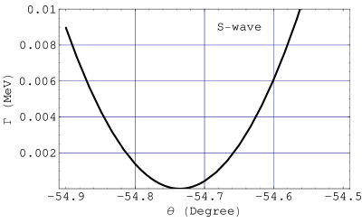
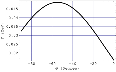
(a)	(b)

Figure 4: The dependence of the partial decay width of $B_{s1}(5830)^{0}\to B^{*+}K^{-}$ on the mixing angle $\theta$. Here (a) and (b) respectively corresponds to S-wave and D-wave decay widths.

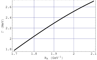
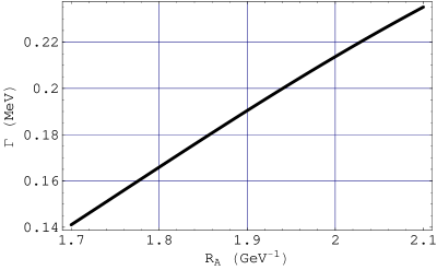
(a)	(b)

Figure 5: The variation of the two-body decay for (a) $B_{s2}^{*}(5840)^{0}\to B^{+}K^{-}$ and (b) $B_{s2}^{*}(5840)^{0}\to B^{*0}K^{-}$ with the factor $R$ of the HO wavefunction of $B_{s2}^{*}(5840)^{0}$.

In Fig. 4 and 5, one shows the dependence of the decay width of $B_{s1}(5830)^{0}\to B^{*+}K^{-}$ on the mixing angle $\theta$ and the variations of the decay widths of $B_{s2}^{*0}(5840)\to B^{0}K^{-},B^{*0}K^{-}$ to the length factor $R$ of HO wavefunction of $B_{s2}^{*0}(5840)$.

As indicated in Fig. 5, to some extent, the result obtained by the ${}^{3}P_{0}$ model is sensitive to $R$ value of HO wavefunction. Since $R$ values can be determined by reproducing the realistic root mean square (RMS) radius when solving the schrödinger equation with the linear potential godfrey , thus we fix the $R$ as the values listed in Table 2, and obtain the partial wave decay width and the two-body decay width of $B_{s1}(5830)^{0}\to B^{*+}K^{-}$ and $B_{s2}^{*0}(5840)\to B^{0}K^{-},B^{*0}K^{-}$, which are listed in Table 3. The numerical result of $B_{s1}(5830)^{0}\to B^{*+}K^{-}$ indicates that the S-wave partial wave decay width can be ignored comparing with that of the D-wave when taking $\theta=-54.7^{\circ}$, which is consistent with the result in quark model.

Mode	$\Gamma_{JL}$ (MeV)	$\Gamma_{two-body}$ (MeV)
$B_{s1}(5830)^{0}\to$	$\Gamma_{10}=4.2\times 10^{-4}$
$B^{*+}K^{-}$	$\Gamma_{12}=4.9\times 10^{-2}$	$4.9\times 10^{-2}$
$B_{s2}^{*}(5840)^{0}\to$
$B^{+}K^{-}$	$\Gamma_{02}=2.3$	2.3
$B_{s2}^{*}(5840)^{0}\to$
$B^{*+}K^{-}$	$\Gamma_{12}=0.2$	0.2

Table 3: The decay widths of two-body strong decays of $B_{s1}(5830)^{0}$ and $B^{*}_{s2}(5840)^{0}$. Here one takes $\theta=-54.7^{\circ}$ for $B_{s1}(5830)^{0}$ decay and adopts the $R$ values listed in Table 2.

In Table 4, we further compare our numerical results of the two-body strong decays of $B_{s1}(5840)$ and $B_{s2}^{*}(5840)$ with the theoretical values calculated by the other models. For the $B_{s1}(5830)^{0}\to B^{*}\bar{K}$ decay rate, our result is far smaller than that from Ref. colangelo and is the same order of magnitude as those of Refs. FM ; zhong . The rates of $B_{s2}(5840)\to B\bar{K}$ process predicted by the different models are consistent with each other at the order of magnitude. For the result of $B_{s2}(5840)\to B^{*}\bar{K}$, one finds that there exists a big difference between the rate from Ref. colangelo and that from our calculation while the results in Refs. EHQ ; zhong are consistent with our result. Thus, we expect the experimental measurement of the two-body decay rates of $B_{s1}(5840)$ and $B_{s2}^{*}(5840)$, which will be helpful not only for clarifying the mist but also for further testing the different effective models. One also notices that the ratio of $\Gamma(B_{s2}^{*}(5840)\to B^{*}\bar{K})$ to $\Gamma(B_{s2}^{*}(5840)\to B\bar{K})$ can provide the useful information to test the model. In this work, we obtain

$$\zeta=\frac{\Gamma(B_{s2}^{*}(5840)\to B^{*}\bar{K})}{\Gamma(B_{s2}(5840)\to B\bar{K})}\sim 8.7\%,$$

which is close to the value $6\%$ from the chiral quark model in Ref. zhong . The results shown in diagrams (a) and (b) of Fig. 5 also indicate the ratio $\zeta$ is a constant basically, which is not varied with the $R$ value in the HO wave function to some extent.

Mode	$\Gamma$ godfrey	$\Gamma$ EHQ	$\Gamma$ FM	$\Gamma$ colangelo	$\Gamma$ zhong	this work
$B_{s1}(5830)\to B^{*}\bar{K}$	-	$<1$	0.28	$3.5$	$0.4\sim 1$	0.098
$B_{s2}^{*}(5840)\to B\bar{K}$	2.6(1.9)	$1$	$7\pm 3^{\S}$	8	$2$	4.6
$B_{s2}^{*}(5840)\to B^{*}\bar{K}$	0.07(0.05)	$<1$		3.2	$0.12$	0.4

Table 4: The comparison between our results of the two-body strong decays of $B_{s1}(5840)$ and $B_{s2}^{*}(5840)$ and the results obtained by the other theoretical groups. Here all of the results are in units of MeV. For the values with and without bracket listed in the second column are from the calculation results of the pseudoscalar emission model and the flux-tube-breaking model, respectively godfrey . ^§ Here $7\pm 3$ MeV is the width sum over the two processes $B_{s2}^{*}(5840)\to B\bar{K},\,B^{*}\bar{K}$ FM .

IV Double pion decays

By our calculation of the two-body strong decays of $B_{s1}(5830)$ and $B_{s2}^{*}(5840)$, we learn that both $B_{s1}(5830)$ and $B_{s2}^{*}(5840)$ are the two states with the narrow widths. Thus, the double pion decay of $B_{s1}(5830)$ and $B_{s2}^{*}(5840)$ is an interesting topic. For estimating their double pion decays, we assume that $B_{s1}(5830)\to B_{s}^{(*)}\pi\pi$ and $B_{s2}^{*}(5840)\to B_{s}^{*}\pi\pi$ can occur via the intermediate scalar state $\sigma$ and $f_{0}(980)$ Ishida:2001pt ; BEH ; lujie ; xiangliu-2860 , which are depicted by Fig. 6. In the following, we consider the $f_{0}(980)$ and $\sigma$ contributions to estimate the double pion decay rates of $B_{s1}(5830)$ and $B_{s2}^{*}(5840)$.

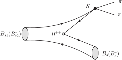
Figure 6: The double pion decay of $B_{s1}(5830)$ and $B_{s2}^{*}(5840)$ via the virtual intermediate state $\sigma$ and $f_{0}(980)$. Here the vertex of $B_{s1}(5830)(B_{s2}^{*}(5840))\to B_{s}^{(*)}\mathcal{S}$ can be depicted by the ${}^{3}P_{0}$ mechanism shown in Fig. 2.

The general expression of the decay width of the two pion decay of $B_{s1}(5830)^{0}$ and $B_{s2}^{*}(5840)^{0}$ is

$$\Gamma_{A\to B+\mathcal{S}\to B+\pi+\pi}=\sum_{\mathcal{S}=\sigma,\,f_{0}}\frac{1}{\pi}\int_{4m_{\pi}^{2}}^{(M_{A}-M_{B})^{2}}\mathrm{d}\,{r}\,\sqrt{r}\,\frac{\Gamma_{A\to B+\mathcal{S}}(r)\,\cdot\,\Gamma_{\mathcal{S}\to\pi+\pi}(r)}{(r-m_{\mathcal{S}}^{2})^{2}+(m_{\mathcal{S}}\Gamma_{S})^{2}},$$ (50)

where $A$ and $B$ denote the initial and final bottom-strange mesons in the two pion process of $B_{s1}(5830)^{0}$ and $B_{s2}^{*}(5840)^{0}$.

The interaction of scalar state ($\mathcal{S}=f_{0}(980),\,\sigma$) with the two pions is described by the effective Lagrangian

$$\mathcal{L}_{\mathcal{S}\pi\pi}=g_{\mathcal{S}}\,{\mathcal{S}}(2\pi^{+}\pi^{-}+\pi^{0}\pi^{0}).$$ (51)

By the total widths of $f_{0}(980)$ ($\Gamma_{f_{0}}=40\sim 100$ MeV) and $\sigma$ ($\Gamma_{\sigma}=600\sim 1000$ MeV), one obtains the values of the coupling constant $g_{f_{0}}=0.83\sim 1.3$ GeV and $g_{\sigma}=2.6\sim 3.4$ GeV. Here we take $m_{\sigma}=600$ MeV PDG . Thus the amplitude $\Gamma_{\mathcal{S}\to\pi+\pi}$ can be expressed as

$$\Gamma_{\mathcal{S}\to\pi+\pi}(r)=\frac{g_{\mathcal{S}}^{2}{\lambda}^{2}}{8\pi}\frac{p_{1}(r)}{r}$$ (52)

with $p_{1}(r)=\sqrt{(r-4m_{\pi}^{2})/4}$. ${\lambda}$ is taken as $\sqrt{2}$ and $1$ for $\pi^{+}\pi^{-}$ and $\pi^{0}\pi^{0}$, respectively.

One uses the ${}^{3}P_{0}$ model to calculate the matrix elements of the transitions of $B_{s1}(5830)^{0}\to B_{s}^{(*)0}\mathcal{S}$ and $B_{s2}^{*}(5840)^{0}\to B_{s}^{*0}\mathcal{S}$. Different from $B_{s1}(5830)^{0}\to B^{*}\bar{K}$ and $B_{s2}^{*}(5840)^{0}\to B\bar{K},B^{*}\bar{K}$ decays discussed in Sec. III, $B_{s1}(5830)^{0}\to B_{s}^{(*)0}\mathcal{S}$ and $B_{s2}^{*}(5840)^{0}\to B_{s}^{*0}\mathcal{S}$ are not only the P-wave decays with $L=1$, but also are relevant to the $s\bar{s}$ quark pair creation. The strength of $s\bar{s}$ creation satisfies $\gamma_{s}=\gamma/\sqrt{3}$ yaouanc-1 due to the flavor dependence of the strength of quark pair creation yaouanc-1 ; strangness . The relevant transition elements are shown in Table 5. The factor $\alpha_{\mathcal{S}}$ in Table 5 is from the flavor wavefunction of $\sigma$ and $f_{0}(980)$

$$\sigma = \frac{1}{\sqrt{3}}(u\bar{u}+d\bar{d}+s\bar{s}),$$ (53)

$$f_{0} = \Big{(}\frac{u\bar{u}+d\bar{d}}{\sqrt{2}}\Big{)}\cos\varphi+s\bar{s}\sin\varphi,$$ (54)

where $\varphi=-48^{\circ}\pm 6^{\circ}$ due to the observation of $f_{0}(980)\to\gamma\gamma$ decay mode f0 . Here $\alpha_{\sigma}=1/\sqrt{3}$ and $\alpha_{f_{0}}=\sin\varphi$. Using eq. (23), we obtain $\Gamma_{A\to B+\mathcal{S}}(r)$ in eq. (50).

Mode	Decay amplitude
$B_{s1}(5830)^{0}\to$	$\alpha_{\mathcal{S}}\big{\{}-\frac{\sqrt{2}}{9}\gamma_{s}\sqrt{E_{A}E_{B}E_{C}}(2I^{0,-1}_{-1,0}+I^{0,0}_{0,0})(-\sin\theta)$
$B_{s}^{0}\mathcal{S}$	$-\frac{2}{9}\gamma_{s}\sqrt{E_{A}E_{B}E_{C}}(I^{-1,0}_{-1,0}+I^{-1,1}_{0,0})\cos\theta\big{\}}$
$B_{s1}(5830)^{0}\to$	$\alpha_{\mathcal{S}}\big{\{}\frac{2}{9}\gamma_{s}\sqrt{E_{A}E_{B}E_{C}}(I^{-1,0}_{-1,0}+I^{-1,1}_{0,0})(-\sin\theta)$
$B_{s}^{*0}\mathcal{S}$	$+\frac{\sqrt{2}}{9}\gamma_{s}\sqrt{E_{A}E_{B}E_{C}}(I^{-1,0}_{-1,0}+I^{-1,1}_{0,0}+2I^{0,-1}_{-1,0}$
	$+I^{0,0}_{0,0})\cos\theta\big{\}}$
$B_{s2}^{*}(5840)^{0}\to$	$-\alpha_{\mathcal{S}}\frac{\sqrt{2}}{9}\gamma_{s}\sqrt{E_{A}E_{B}E_{C}}[I^{-1,0}_{-1,0}+I^{-1,1}_{0,0}-2I^{0,-1}_{-1,0}$
$B_{s}^{*0}\mathcal{S}$	$-I^{0,0}_{0,0}]$

Table 5: The decay amplitude of the three-body strong decays of $B_{s1}(5830)^{0}$ and $B^{*}_{s2}(5840)^{0}$. Here functions $I_{M_{L_{B}},M_{L_{C}}}^{M_{L_{A}},m}$ are listed in the appendix.

In Fig. 7, the dependence of the double pion decay of $B_{s1}(5830)^{0}$ on the mixing angle is given. We also present the variation of $B_{s2}^{*}(5840)^{0}\to B_{s}^{*0}\pi^{+}\pi^{-}$ with the parameter $R$ of the HO wavefunction of $B_{s2}^{*}(5840)^{0}$ in Fig. 8. Here the shadow in Figs. 7 and 8 is the possible value of the decay width. The decay width of the double pion strong decays of $B_{s1}(5830)^{0}$ and $B^{*}_{s2}(5840)^{0}$ are shown in Table 6 when taking the mixing angle $\theta=-54.7^{\circ}$ and the $R$ value listed in Table 2.

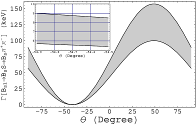
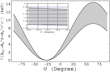
(a)	(b)

Figure 7: (a) The variation of the decay width of $B_{s1}(5830)^{0}\to B_{s}^{0}\pi^{+}\pi^{-}$ with the mixing angle $\theta$, $g_{f_{0}}=0.83\sim 1.3$ GeV and $g_{\sigma}=2.6\sim 3.4$ GeV; (b) For the case of $B_{s1}(5830)^{0}\to B_{s}^{*0}\pi^{+}\pi^{-}$. In the left-top diagrams of both (a) and (b), we show the enlarged detail around $\theta=-54.7^{\circ}$.

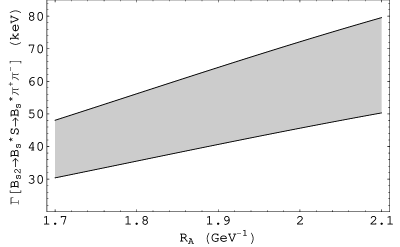
Figure 8: The dependence of decay width of $B_{s2}^{*}(5840)^{0}\to B_{s}^{*0}\pi^{+}\pi^{-}$ on the $R$ value of the HO wavefunction of $B_{s2}^{*}(5840)^{0}$, $g_{f_{0}}=0.83\sim 1.3$ GeV and $g_{\sigma}=2.6\sim 3.4$ GeV.

Mode	$\Gamma_{\pi^{+}\pi^{-}}$	$\Gamma_{\pi^{+}\pi^{-}}^{\sigma}$	$\Gamma_{\pi^{+}\pi^{-}}^{f_{0}(980)}$	$\Gamma_{\pi^{0}\pi^{0}}$	$\Gamma_{\pi^{0}\pi^{0}}^{\sigma}$	$\Gamma_{\pi^{0}\pi^{0}}^{f_{0}(980)}$
$B_{s1}(5830)^{0}\to B_{s}^{0}\pi\pi$	$5.6\sim 8.7$	$1.0\sim 1.1$	$4.5\sim 7.6$	$6.1\sim 9.6$	$1.1\sim 1.2$	$4.9\sim 8.3$
$B_{s1}(5830)^{0}\to B_{s}^{*0}\pi\pi$	$2.0\sim 3.1$	$0.37\sim 0.41$	$1.6\sim 2.7$	$2.3\sim 3.7$	$0.44\sim 0.49$	$1.9\sim 3.2$
$B_{s2}^{*}(5840)^{0}\to B_{s}^{*0}\pi\pi$	$41.7\sim 65.9$	$7.8\sim 8.7$	$33.8\sim 57.2$	$48.1\sim 76.1$	$9.1\sim 10.1$	$39.1\sim 66.1$

Table 6: The decay widths of the double pion strong decays of $B_{s1}(5830)^{0}$ and $B^{*}_{s2}(5840)^{0}$. Here one takes $\theta=-54.7^{\circ}$ for $B_{s1}(5830)^{0}$ decay, and fixes all $R$’s with the typical values listed in Table 2. $\Gamma^{\sigma}_{\pi\pi}$ and $\Gamma^{f_{0}(980)}_{\pi\pi}$ show the separate contributions of $\sigma$ and $f_{0}(980)$. All results are in units of keV.

V Short summary

In this work, we study the two-body strong decays and the double pion decays of the newly observed $B_{s1}(5830)$ and $B_{s2}^{*}(5840)$ in the framework of the ${}^{3}P_{0}$ model. Our result shows that the two-body strong decay widths of $B_{s1}(5830)$ and $B_{s2}^{*}(5840)$ are about 98 keV and 5.0 MeV, respectively, when we choose the fixed parameter presented in Sec. III. $B_{s1}(5830)$ and $B_{s2}^{*}(5840)$ are of narrow decay widths, which is due to the limitation of phase space and the domination of D-wave decay for the decays of $B_{s1}(5830)$ and $B_{s2}^{*}(5840)$ into $B\bar{K}$ and $B^{*}\bar{K}$. Since the two-body strong decay is the dominant decay mode for $B_{s1}(5830)$ and $B_{s2}^{*}(5840)$, thus one expects that the total decay widths of $B_{s1}(5830)$ and $B_{s2}^{*}(5840)$ are almost not far away from their two-body decay widths at the order of magnitude.

We also calculate the double pion decay of $B_{s1}(5830)$ and $B_{s2}^{*}(5840)$ by assuming the double pion from $\sigma$ and $f_{0}(980)$. The double pion decay widths are of the order of a few keV and up to the order of magnitude of a few tens of keV for $B_{s1}(5830)$ and $B_{s2}^{*}(5840)$, respectively. Although the double pion decay widths of $B_{s1}(5830)$ and $B_{s2}^{*}(5840)$ are smaller than those of their two-body strong decay, the double pion decay rates of $B_{s1}(5830)$ and $B_{s2}^{*}(5840)$ are sizable. Thus we suggest future experiments to search the double pion decay mode of $B_{s1}(5830)$ and $B_{s2}^{*}(5840)$.

Up to now, the experimental values of the total width of $B_{s1}(5830)$ and $B_{s2}^{*}(5840)$ have not been given. To some extent, our study is instructive for finally determining the total width of the two newly observed $B_{s}$ meson in the following experiments. Of course it is also a good way to further test the ${}^{3}P_{0}$ model and other effective models.

Appendix

When $L_{A}=1$ and $L_{B}=L_{C}=0$, the spatial overlap $I_{M_{L_{B}},M_{L_{C}}}^{M_{L_{A}},m}$ is simplified as $\delta^{3}(\textbf{K}_{B}+\textbf{K}_{C})I_{m^{\prime}n^{\prime}}(\textbf{K})$, where

$$I_{m^{\prime}n^{\prime}}(\textbf{K}) = \left(i\frac{\sqrt{2}}{\pi^{3/4}}\right)\left(\frac{1}{\pi^{3/4}}\right)^{2}\left(\frac{1}{2}\right)^{3}\,\left(\frac{3}{4\pi}\right)^{1/2}R_{A}^{5/2}R_{B}^{3/2}R_{C}^{3/2}\exp\left(-\frac{1}{8}\zeta^{2}\textbf{K}^{2}\right)$$ (55)

$$\times\int{\rm d}\mathbf{k}\left[-k_{m^{\prime}}k_{n^{\prime}}+(1-\eta^{2})K_{m^{\prime}}K_{n^{\prime}}\right]\,\exp\left(-\frac{1}{8}\Delta^{2}\mathbf{k}^{2}\right).$$

The parameters $\Delta$, $\zeta$ and $\eta$ are defined as

$$\Delta^{2}=R_{A}^{2}+R_{B}^{2}+R_{C}^{2},\,\,\eta=\frac{R_{A}^{2}+\xi_{1}R_{B}^{2}+\xi_{2}R_{C}^{2}}{R_{A}^{2}+R_{B}^{2}+R_{C}^{2}},$$

$$\zeta^{2}=R_{A}^{2}+\xi_{1}^{2}R_{B}^{2}+\xi_{2}^{2}R_{C}^{2}-\frac{(R_{A}^{2}+\xi_{1}R_{B}^{2}+\xi_{2}R_{C}^{2})^{2}}{R_{A}^{2}+R_{B}^{2}+R_{C}^{2}}.$$

The $\xi_{1}$ and $\xi_{2}$ represent the mass difference effects in mesons

$$\xi_{1}=\frac{m_{3}-m_{1}}{m_{3}+m_{1}},\quad\xi_{2}=\frac{m_{4}-m_{2}}{m_{4}+m_{2}},\quad m_{3}=m_{4}.$$

Here $m_{i}$ denotes the quark mass. In this work, we take $m_{u}=m_{d}=0.22$ GeV, $m_{s}=0.419$ GeV, $m_{b}=1.977$ GeV godfrey .

The concrete calculations of the integration are trivial. After choosing the direction of K along $z$ axis, we obtain the expressions $I_{\pm,0}$ in Table 1

$$I_{\pm}=I_{1-1}=I_{-11}$$

$$\quad=i\frac{8\sqrt{3}}{\pi^{5/4}\Delta^{5}}\left(R_{A}^{5/2}R_{B}^{3/2}R_{C}^{3/2}\right)\exp\left(-\frac{1}{8}\zeta^{2}\textbf{K}^{2}\right),$$

$$I_{0}=I_{00}=i\frac{8\sqrt{3}}{\pi^{5/4}\Delta^{5}}\left(R_{A}^{5/2}R_{B}^{3/2}R_{C}^{3/2}\right)$$

$$\quad\times\exp\left(-\frac{1}{8}\zeta^{2}\textbf{K}^{2}\right)\left[-1+\frac{1}{4}(1-\eta^{2})\Delta^{2}\textbf{K}^{2}\right].$$

When $L_{A}=L_{B}=1$ and $L_{C}=0$, the spatial overlaps are of the form $\delta^{3}(\textbf{K}_{B}+\textbf{K}_{C})\,I^{m^{\prime},n^{\prime}}_{\ell^{\prime},0}(\textbf{K})$. Here $I^{m^{\prime},n^{\prime}}_{\ell^{\prime},0}$ is abbreviated as $I_{m^{\prime}n^{\prime}\ell^{\prime}}$ with definition

$$I_{m^{\prime}n^{\prime}\ell^{\prime}}$$

$$=\left(\frac{\sqrt{2}}{\pi^{3/4}}\right)^{2}\left(\frac{1}{\pi^{3/4}}\right)\left(\frac{3}{4\pi}\right)^{1/2}\left(\frac{1}{2}\right)^{4}R_{A}^{5/2}R_{B}^{5/2}R_{C}^{3/2}$$

$$\quad\times\exp\left(-\frac{1}{8}\zeta^{2}\textbf{K}^{2}\right)\int{\rm d}\mathbf{k}\,\big{[}-(\xi_{1}-\eta)k_{m^{\prime}}k_{n^{\prime}}K_{-\ell^{\prime}}$$

$$\quad(1+\eta)k_{m^{\prime}}k_{-\ell^{\prime}}K_{n^{\prime}}-(1-\eta)k_{n^{\prime}}k_{-\ell^{\prime}}K_{m^{\prime}}$$

$$\quad+(1-\eta^{2})(\xi_{1}-\eta)K_{m^{\prime}}K_{n^{\prime}}K_{-\ell^{\prime}}\,\big{]}\exp\left(-\frac{1}{8}\Delta^{2}\mathbf{k}^{2}\right).$$

The explicit results are

$$I_{1-10}=I_{-110}=\frac{4\sqrt{6}}{\pi^{7/4}\Delta^{5}}\left(R_{A}^{5/2}R_{B}^{5/2}R_{C}^{3/2}\right)\,|\textbf{K}|\exp\left(-\frac{1}{8}\zeta^{2}\textbf{K}^{2}\right)\left[-\eta+\xi_{1}\right],$$ (57)

$$I_{101}=I_{-10-1}=\frac{4\sqrt{6}}{\pi^{7/4}\Delta^{5}}\left(R_{A}^{5/2}R_{B}^{5/2}R_{C}^{3/2}\right)\,|\textbf{K}|\exp\left(-\frac{1}{8}\zeta^{2}\textbf{K}^{2}\right)\left[-1-\eta\right],$$ (58)

$$I_{011}=I_{0-1-1}=\frac{4\sqrt{6}}{\pi^{7/4}\Delta^{5}}\left(R_{A}^{5/2}R_{B}^{5/2}R_{C}^{3/2}\right)\,|\textbf{K}|\exp\left(-\frac{1}{8}\zeta^{2}\textbf{K}^{2}\right)\left[-\eta+1\right],$$ (59)

$$I_{000}=\frac{4\sqrt{6}}{\pi^{7/4}\Delta^{5}}\left(R_{A}^{5/2}R_{B}^{5/2}R_{C}^{3/2}\right)|\textbf{K}|\exp\left(-\frac{1}{8}\zeta^{2}\textbf{K}^{2}\right)$$

$$\quad\quad\quad\times\left[-\xi_{1}+3\eta+\frac{1}{4}(1-\eta^{2})(\xi_{1}-\eta)\Delta^{2}\textbf{K}^{2}\right].$$ (60)

References

(1)
B. Aubert et al. [BABAR Collaboration],
Phys. Rev. Lett. 90, 242001 (2003).
(2)
P. Krokovny et al. [Belle Collaboration],
Phys. Rev. Lett. 91, 262002 (2003).
(3)
D. Besson et al. [CLEO Collaboration],
Phys. Rev. D 68, 032002 (2003)
[Erratum-ibid. D 75, 119908 (2007)].
(4)The CLEO
Collaboration, D. Besson et al., Phys. Rev. D 68, 032002
(2003).
(5)Belle Collaboration, Y.Mikami et al., Phys. Rev. Lett. 92,
012002 (2004); Belle Collaboration, A. Drutskoy et al., Phys. Rev.
Lett. 94, 061802 (2005); Belle Collaboration, P. Krokovny et
al., AIP Conf. Proc. 717, 475-484 (2004); FOCUS
Collabortation, E. W. Vaandering, arXiv: hep-ex/0406044; Babar
Collaboration, B. Aubert et al., Phys. Rev. Lett. 93, 181801
(2004); Babar Collaboration, B. Aubert et al., Phys. Rev. D 69, 031101 (2004); Babar Collaboration, G. Calderini et al.,
arXiv: hep-ex/0405081; Babar Collaboration, B. Aubert et al.,
arXiv: hep-ex/0408067.
(6)Babar Collaboration, B. Aubert et al., Phys. Rev. Lett. 97, 222001 (2006).
(7)Belle Collaboration, K. Abe et al., arXiv:
hep-ex/0608031.
(8)Belle Collaboration, J. Brodzicka et al.,
Phys. Rev. Lett. 100, 092001 (2008).
(9)BABAR Collaboration, B. Aubert et al., Phys. Rev. Lett. 98, 012001
(2007).
(10)BELLE Collaboration, K. Abe et al., Phys. Rev. Lett. 98, 262001 (2007).
(11)BABAR Collaboration, B. Aubert et al.,
arXiv: hep-ex/0607042.
(12)BELLE Collaboration, R. Chistov et al.,
Phys. Rev. Lett. 97, 162001 (2006).
(13)Babar Collaboration, T. Schröder, talk given at the EPS High Energy Physics Conference,
Manchester, July, 2007.
(14)BABAR Collaboration, B. Aubert et al., Phys. Rev. Lett. 97, 232001
(2006).
(15)CLEO Collaboration, M. Artuso et al., Phys. Rev.
Lett. 86, 4479 (2001).
(17)I. V. Gorelov,
J. Phys. Conf. Ser. 69, 012009 (2007).
(18)D0 Collaboration, V. Abazov et al., Phys. Rev. Lett. 99, 052001 (2007).
(19)D. Litvintsev, on behalf of the CDF Collaboration, seminar at Fermilab, June
15, 2007, http://theory.fnal.gov/jetp/talks/litvintsev.pdf.
(20)CDF Collaboration, T. Aaltonen et al., Phys. Rev. Lett. 99, 052002 (2007).
(21)C. Amsler et al., Phys. Lett. B 667, 1 (2008).
(22)CDF Collaboration, T. Aaltonen et al., Phys. Rev.
Lett. 100, 082001 (2008).
(23)D0 Collabotation, V.M. Abazov et al.,
Phys. Rev. Lett. 100, 082002 (2008).
(24)S. Godfrey and R. Kokoski, Phys. Rev. D 43, 1679 (1991).
(25)E.J. Eichten, C.T. Hill and C. Quigg, Phys. Rev.
Lett. 71, 4116 (1993).
(26)D. Ebert, V.O. Galkin and R.N. Faustov, Phys. Rev. D
57, 5663 (1998).
(27)M.Di Pierro and E.J. Eichten, Phys. Rev. D
64, 114004 (2001).
(28)A.F. Falk and T. Mehen, Phys. Rev. D 53, 231
(1996).
(29)A.M. Green, J. Koponen, C. Michael, C. McNeile and G.
Thompson, Phys. Rev. D 69, 094505 (2004).
(30)P. Colangelo, F.De Fazio and R. Ferrandes,
Nucl. Phys. B, Proc. Suppl. 163, 177 (2007).
(31)T. Matsuki, T. Morii, K. Sudoh, Prog. Theor. Phys. 117, 1077-1098
(2007).
(32)X.H. Zhong and Q. Zhao, Phys. Rev. D 78, 014029
(2008).
(33)Z.G. Luo, X.L. Chen, X. Liu and S.L. Zhu,
arXiv:0805.4074 [hep-ph].
(34) L. Micu, Nucl. Phys. B 10, 521 (1969).
(35)A. Le Yaouanc, L. Oliver, O. Pène and J. Raynal,
Phys. Rev. D 8, 2223 (1973); D 9, 1415 (1974); D 11, 1272 (1975); Phys. lett. B 71, 57 (1977); B 71,
397 (1977); .
(36)A. Le Yaouanc, L. Oliver, O. Pène and J. Raynal,
Phys. Lett. B 72, 57 (1977).
(37) A. Le Yaouanc, L. Oliver, O. Pène and J. Raynal,
Hadron Transitions in the Quark Model, Gordon and Breach
Science Publishers, New York, 1987.
(38)E. van Beveren, C. Dullemond and G. Rupp, Phys. Rev. D 21, 772 (1980);
E. van Beveren, G. Rupp, T.A. Rijken and C. Dullemond, Phys. Rev.
D 27, 1527 (1983).
(39)R. Bonnaz, B. Silvestre-Brac and C. Gignoux, Eur. Phys. J. A 13, 363-376 (2002) .
(40)W. Roberts and B. Silvestre-Brac, Few-Body Systems, 11, 171 (1992).
(41) H.G. Blundell and S. Godfrey, Phys. Rev. D 53, 3700
(1996).
(42)P.R. Page, Nucl. Phys. B 446, 189 (1995); S. Capstick and N.
Isgur, Phys. Rev. D 34, 2809 (1986).
(43)S. Capstick and W. Roberts, Phys. Rev. D 49, 4570 (1994).
(44)E.S. Ackleh, T. Barnes and E.S. Swanson, Phys. Rev. D54, 6811 (1996).
(45)H.Q. Zhou, R.G. Ping and B.S. Zou, Phys. Lett. B 611, 123
(2005).
(46)X.H. Guo, H.W. Ke, X.Q. Li, X. Liu and S.M. Zhao, Commun. Theor. Phys. 48, 509-518 (2007).
(47)
F. E. Close and E. S. Swanson,
Phys. Rev. D 72, 094004 (2005).
(48)J. Lu, W.Z. Deng, X.L. Chen and S.L. Zhu, Phys. Rev. D 73 054012,
(2006).
(49)B. Zhang, X. Liu, W.Z. Deng and S.L. Zhu, Eur. Phys.
J. C 50, 617 (2007).
(50)C. Chen, X.L. Chen, X. Liu, W.Z. Deng and S.L.
Zhu, Phys. Rev. D 75, 094017 (2007); X. Liu, C. Chen, W.Z.
Deng and X.L. Chen, Chin. Phys. C 32, 424-427 (2008),
arXiv:0710.0187 [hep-ph].
(51)
D. M. Li and B. Ma,
Phys. Rev. D 77, 074004 (2008);
D. M. Li and B. Ma,
Phys. Rev. D 77, 094021 (2008);
D. M. Li and S. Zhou,
Phys. Rev. D 78, 054013 (2008);
D. M. Li and S. Zhou,
arXiv:0811.0918 [hep-ph].
(52)C. Hayne and N. Isgur, Phys. Rev. D 25, 1944 (1982).
(53)M. Jacob and G. C. Wick, Ann. Phys. 7, 404 (1959).
(54)Y. B. Dai and Shi-Lin Zhu, Phys. Rev. D 58, 074009
(1998).
(55)S. Godfrey and N. Isgur, Phys. Rev. D 32, 189
(1985).
(56)F.E. Close and E.S. Swanson, Phys. Rev. D 72, 094004
(2005).
(57)R. Kokoski and N. Isgur, Phys. Rev. D 35, 907
(1987).
(58)
M. Ishida, S. Ishida, T. Komada and S. I. Matsumoto,
Phys. Lett. B 518, 47 (2001).
(59)W.A. Bardeen, E.J. Eichten and C.T. Hill, Phys. Rev. D 68, 054024 (2003).
(60)H.G. Dosch and D. Gromes, Z. Phys. C 34,
139 (1987).
(61)A.V. Anisovich, V.V. Anisovich and V.A. Nikonov, Eur. Phys. J A 12, 103
(2001).