Analysis of self-organized criticality in Ehrenfest’s dog-flea model

Abstract

The self-organized criticality in Ehrenfest’s historical dog-flea model is analyzed by simulating the underlying stochastic process. The fluctuations around the thermal equilibrium in the model are treated as avalanches. We show that the distributions for the fluctuation length differences at subsequent time steps are in the shape of a $q$-Gaussian (the distribution which is obtained naturally in the context of nonextensive statistical mechanics) if one avoids the finite size effects by increasing the system size. We provide a clear numerical evidence that the relation between the exponent $\tau$ of avalanche size distribution obtained by maximum likelihood estimation and the $q$ value of appropriate $q$-Gaussian obeys the analytical result recently introduced by Caruso et al. [Phys. Rev. E 75, 055101(R) (2007)]. This rescues the $q$ parameter to remain as a fitting parameter and allows us to determine its value a priori from one of the well known exponents of such dynamical systems.

Introduction:   The term self-organized criticality (SOC) was first introduced by Bak, Tang, and Wiesenfeld (BTW) in 1987 Bak et al. (1987). In their well known paper, the so-called BTW sandpile model was used to demonstrate that the dynamics which gives rise to the power-law correlations seen in the non-equilibrium steady states must not involve any fine-tuning of parameters. Namely, systems under their natural evolution are driven at a very slow rate until one of their elements reaches a threshold, i.e., statistically stationary state, and this triggers a burst of activity (avalanche) which occurs on a very short time scale. When the avalanche is over, the system evolves again according to the slow drive until a next avalanche is triggered. The activity of the system in this way consists of a series of avalanches. There are many systems where the SOC paradigm has been applied, e.g. earthquakes, noise with $1/f$ power spectrum, brain activity, river networks, biological evolution of interacting species, traffic jams etc. Jensen (1988).

Following the BTW sandpile model a great variety of models from the deterministic and stochastic to the dissipative and conservative have been introduced which exhibit the phenomenon of SOC (for an overview, see Dhar (2006) and references therein). In 1996, a random neighbor version of the original BTW sandpile model was presented by Flyvbjerg Flyvbjerg (1996). In this work, it was emphasized that a self-organized critical system is a driven, dissipative system consisting of a medium (sandpile) which has disturbance propagating through it, causing a modification of the medium, such that eventually the medium is in a critical state, and the medium is modified no more. Moreover, it was shown by way of random neighbor sandpile model that a dynamical system with only two degrees of freedom can be self-organized critical and as it is the case in fluctuation phenomena, the dynamics is described by a master equation which can be partially solved analytically.

Soon after Flyvbjerg’s work Nagler et al. studied the conservative variant of random neighbor sandpile model which is neither extended nor dissipative with regard to the amount of sand in the system but still shows SOC with nontrivial exponents Nagler et al. (1999); Hauert et al. (2004). This kind of analysis is not restricted to nonspatial systems and available also for spatial systems like one-dimensional cellular automata Nagler and Claussen (2005). The dynamics of the model described by Nagler et al. is given on a Fokker-Planck equation by introducing appropriate scaling variables. The avalanche size distribution which is readily obtained by solving the Fokker-Planck equation at an absorbing boundary exhibits a power-law regime followed by an exponential tail. Their model is an adaptation of the famous dog-flea model introduced by Ehrenfest in 1907 Ehrenfest and Ehrenfest (1907). This model can be considered as a zero-dimensional nonspatial prototype SOC model and its dynamics is different from most of the standard SOC models which are $N$-dimensional spatial systems.

The dog-flea model is a simple but typical example of generation-recombination Markov chain Bhattacharya and Waymire (1990) describing the process of approaching an equilibrium state in a large set of uncoupled two state systems together with fluctuations (avalanches) around this state. For an even number of states, the transition probability of fluctuations of the discrete time version was calculated by Kac Kac (1947) (see also Wax (1954)). An identification of the model as a random walk on a Bethe lattice is studied in Ref. Hughes and Sahimi (1994). Furthermore, it has recently been shown that the dog-flea model, formulated as a continuous time Markov chain, is a representation of a spin in a magnetic field Lemmens (1996). Such a representation is used to estimate the blocking temperature in molecular nano-magnets Bakar and Lemmens (2005).

In this work, we will be analyzing the SOC in the dog-flea model through simulation of the underlying stochastic process that describes the natural evolution of the model. The analysis method that we use has recently been presented by Caruso et al. to interpret the SOC in the limited number of earthquakes (up to 689 000) taken from World and Northern California catalogs for the periods 2001-2006 and 1966-2006, respectively Caruso et al. (2007). Using the same line of thought, it is our aim to analyze the SOC feature of the dog-flea model through the time series of the fluctuation length. The simplicity of the dynamics of the dog-flea model enables us to obtain a large number of fluctuations for different system sizes in a reasonable computing time (i.e., we consider up to $2\times 10^{9}$ fluctuations). Thus, the obtained critical exponents for the model are very precise as it will be discussed in coming sections. This analysis enables us to accomplish our main task, which is to provide the first rigorous numerical example where the relationship, proposed by Caruso et al., between the exponent $\tau$ of avalanche size distribution and the $q$ value of appropriate $q$-Gaussian (the distribution which is obtained naturally in the context of nonextensive statistical mechanics) Tsallis (1988). This will be very appealing also from nonextensive statistical mechanics point of view since this treatment makes the $q$ parameter to be determined a priori, which is a situation achieved rarely up to now.

The model and numerical procedure:   The dynamics of the dog-flea model has simple rules. The model has $N$ dynamical sites represented by the total number of fleas shared by two dogs (dog $A$ and dog $B$). Suppose that there are $N_{A}$ fleas on dog $A$ and $N_{B}$ fleas on dog $B$ leading to a population of fleas $N=N_{A}+N_{B}$. For convenience, $N$ is assumed to be even. In every time step, a randomly chosen flea jumps from one dog to the other. Thus, we have $N_{A}\rightarrow N_{A}\pm 1$ and $N_{B}\rightarrow N_{B}\mp 1$. The procedure is repeated for an arbitrary number of times. In long time run, the mean number of fleas on both dog $A$ and dog $B$ converges to the equilibrium value, $\langle N_{A}\rangle=\langle N_{B}\rangle=N/2$ with the fluctuations around it. A single fluctuation is described as a process that starts once the number of fleas on one of the dogs becomes larger (or smaller) than the equilibrium value $N/2$ and stops when it gets back to it for the first time. Thus, the end of one fluctuation specifies the start of the subsequent one. The length ($\lambda$) of a fluctuation is determined by the number of time steps elapsed until the fluctuation ends.

It is straightforward to obtain the master equation of the process that describes the time evolution of the probability to find a specified number of fleas on one of the dogs. Assuming that after $t$ steps there are $N_{A}(t)=\ell$ fleas on dog $A$, at the subsequent time step there are only two possibilities, $\ell\rightarrow\ell+1$ or $\ell\rightarrow\ell-1$ with the transition probabilities $W(\ell+1|\ell)=(N-\ell)/N$ and $W(\ell-1|\ell)=\ell/N$, respectively. Then, the time evolution of the probability $P(\ell,\,t)$ to find $\ell$ fleas on dog $A$ at time $t$ obeys the following master equation,

$$P(\ell,\,t+1)=\frac{\ell+1}{N}P(\ell+1,\,t)+\frac{N-\ell+1}{N}P(\ell-1,\,t).$$ (1)

Introducing appropriate scaling variables Eq. (1) can be written in the form of a Fokker-Planck equation by which the fluctuation distribution is reviewed analytically Nagler et al. (1999).

Distribution of fluctuation length and returns:   As it was first demonstrated by BTW sandpile model, a generic signature of SOC is the presence of a power-law as well as finite size scaling in the size or the duration distribution of the avalanches. Recently, a power-law regime following an exponential tail in the fluctuation length distribution for the Ehrenfest’s dog-flea model has been reported for a very limited system size (i.e., $N=2500$) Nagler et al. (1999). In our paper, in order to analyze the SOC in the dog-flea model through the fluctuation length distribution we simulate the corresponding stochastic process for seven different values of $N$ namely, $N=10^{2},\,10^{3},\,5\times 10^{3},\,10^{4},\,10^{5},\,10^{6},$ and $10^{7}$. For convenience, let us group the first four different system sizes as “small $N$s” and the remaining sizes as “large $N$s”. In Fig. 1(a) and (b) we plot the distribution of the fluctuation length time-series $\lambda(t)$ for the small $N$s and large $N$s, respectively. In order to have good statistics $10^{9}$ fluctuations for the small $N$s group and $2\times 10^{9}$ fluctuations for the large $N$s group have been considered. In both cases the fluctuation distributions have a power-law regime, $P(\lambda)\sim\lambda^{-\tau}$ while in the small $N$s group the power-law regime is followed by an exponential decay because of the finite-size effect. For the small $N$s group one can control if the fluctuation length distribution $P(\lambda)$ obeys the following finite size scaling behavior,

$$P(\lambda)\sim\frac{1}{N^{\gamma}}f\left(\frac{\lambda}{N^{\zeta}}\right),$$ (2)

where $f$ is a suitable scaling function and $\gamma$ and $\zeta$ are critical exponents describing the scaling of the distribution function. In the inset of Fig. 1(a), a clear data collapse of $P(\lambda)$ is shown for the small $N$s group (i.e., $N=10^{2},\,10^{3},\,5\times 10^{3},\,$ and $10^{4}$). This data collapse indicates that the fluctuation length distributions of small $N$s satisfy the finite size scaling hypothesis very well. The obtained critical exponents are $\gamma\simeq 1.517$ and $\zeta=1$. As it is seen from Fig. 1(b), these values of critical exponents are in agreement with the finite size scaling hypothesis since for asymptotically large $N$, $P(\lambda)\sim\lambda^{-\tau}$ with $\tau=\gamma/\zeta\simeq 1.517$. The value of $\tau$ is obtained by the maximum likelihood estimation (MLE) and this method enables us to determine this exponent of the model as accurate as $\pm 1.156\times 10^{-5}$ Newman (2005).

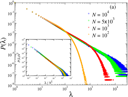
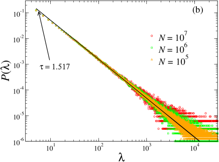
Figure 1: (color online) Fluctuation length distributions for the small $N$s and for the large $N$s groups are given in (a) and (b), respectively. In the inset of (a), we also present data collapse of finite size scaling given in Eq. (2) for small $N$s group. The critical exponents derived from the fit are $\gamma\simeq 1.517$ and $\zeta=1$. The full black line in (b) represents the fitting curve of the distribution with slope $\tau\simeq 1.517$ which has been obtained by maximum likelihood estimation. The distributions have an arbitrary normalization such that $P(\lambda=1)=1$.

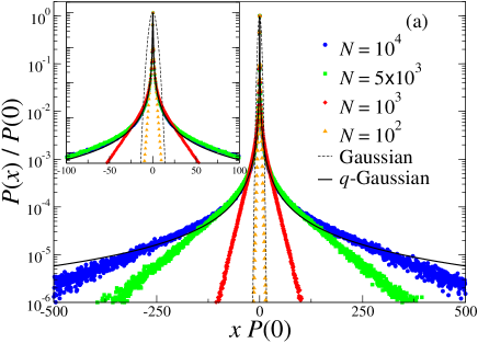
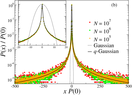
Figure 2: (color online) The distributions of returns, i.e., the fluctuation length differences $\Delta\lambda(t)=\lambda(t+1)-\lambda(t)$, normalized by introducing the variable $x=\Delta\lambda-\langle\Delta\lambda\rangle$ are shown in (a) for the small $N$s group and in (b) for the large $N$s group. For comparison, standard Gaussian and $q$-Gaussian curves are drawn by black dashed and full lines, respectively. See text for further details. In insets, the central parts of the distributions are emphasized.

Now we are at the position to introduce the distribution of returns, i.e., the differences between fluctuation lengths obtained at consecutive time steps, as $\Delta\lambda(t)=\lambda(t+1)-\lambda(t)$. It should also be noted that, in order to have zero mean, the returns are normalized by introducing the variable $x$ as

$$x=\Delta\lambda-\langle\Delta\lambda\rangle,$$ (3)

where $\langle\cdots\rangle$ stays for the mean value of the given data set. The signal of the distribution of returns reveals very interesting results on the criticality of the dog-flea model. This approach is used in recent studies on turbulence Menech and Stella (2002) and the time-series of real earthquakes Caruso et al. (2007).

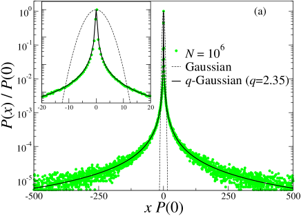
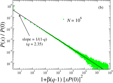
Figure 3: (color online) (a) Distribution of returns for a representative case of large $N$s group ($N=10^{6}$) is given by full green circles. The $q$-Gaussian curve with $q=2.35$ and $\beta=35$ is shown by full black line. This value of the $q$ is obtained by substituting $\tau=1.517$ into Eq. (6). A standard Gaussian curve is drawn by dashed black line for comparison. In the inset, the central part of the distribution is given in order to emphasize that the distribution approaches almost perfectly to the $q$-Gaussian not only in the tails but also in the center. (b) In order to better visualize how well the used $q$-Gaussian approaches to the distribution, we plot the same $P(x)$ versus $1+\beta(q-1)x^{2}$. A straight line with a slope $1/(1-q)$ is expected for a perfectly $q$-Gaussian shaped distribution. Data points (green circles) and the slope with $q=2.35$ (black line) constitute a clear evidence towards this tendency.

In Fig. 2, we plot the distribution of the returns $\Delta\lambda(t)$ obtained from $10^{9}$ fluctuations for each different system sizes in the small $N$s group (a), whereas in the group of large $N$s (b) $2\times 10^{9}$ fluctuations are considered. What is common for both cases is that none of them has return distributions which can be approached by a Gaussian. As the system size $N$ increases, leading to a longer power-law regime in the fluctuation length distribution, the return distribution curves become to exhibit a convergence to a kind of fat tailed distribution. When the system size is large enough, the exponential decay of the fluctuation length distribution (see Fig. 1(b)) is postponed to larger sizes and the finite size effects get invisible up to more than four decades. In this case the distribution of the returns can be fitted by a $q$-Gaussian given by

$$P(x)=P(0)[(1+\bar{\beta}(q-1)x^{2}]^{1/(1-q)},$$ (4)

where $\bar{\beta}$ characterizes the width of the distribution and $q$ is the index of nonextensive statistical mechanics Tsallis (1988) (black full lines in Figs. 2(a) and (b)). In Eq. (4), $q\neq 1$ indicates a departure from the Gaussian shape while normal Gaussian distribution can be recovered again in the $q\rightarrow 1$ limit. Here, it is worth mentioning that our results in Fig. 2 clearly show the connection between criticality and the appearance of $q$-Gaussian, namely, wider the critical regime persists, longer the tails of returns distribution follow $q$-Gaussian. This kind of interpretation might also be useful in understanding the difference between two recent experimental works on velocity distributions in optical lattices Jersblad et al. (2004); Dougles et al. (2006). In Jersblad et al. (2004), velocity distributions are found to approach a double-Gaussian shape, whereas in Dougles et al. (2006) they are reported to converge to a $q$-Gaussian. The reason for this discrepancy seen in the results of essentially the same experiment might be that in the latter the system may be set exactly at the criticality, whereas in the former it is not.

At this point, we should recall the important result reported by Caruso et al. Caruso et al. (2007) relating the $\tau$ exponent of the avalanche size distribution with the $q$ parameter of the $q$-Gaussian. As it was emphasized in their work, if there is no correlation between the size of two events, the probability of obtaining the difference $\Delta\lambda=\lambda(t+\delta)-\lambda(t)$ ($\delta$ is an integer describing the correlation length and in our case $\delta=1$) is given by

$$P(\Delta\lambda)=K\frac{\epsilon^{-(2\tau-1)}}{2\tau-1}{{}_{2}F_{1}}\left(\tau,2\tau-1;2\tau;-\frac{|\Delta\lambda|}{\epsilon}\right),$$ (5)

where $K$ is a normalization factor, $\epsilon$ is a small positive value and ${{}_{2}F_{1}}$ is the hypergeometric function. The curve of this $\tau$ dependent probability density function $P(\Delta\lambda)$ can be approached by means of $q$-Gaussian with $\epsilon$-independent $q$ value. In Ref. Caruso et al. (2007), by evaluating Eq. (5) for various values of $\tau$, a relation between the power-law exponent $\tau$ and $q$ is reported as

$$q=e^{1.19\tau^{-0.795}}.$$ (6)

Although this relation is obtained in Caruso et al. (2007) by Caruso et al., they could not check its validity since the earthquake data that they analyzed was not adequate to obtain the $\tau$ value with high precision. Consequently, they still used $q$ parameter as a fitting parameter. On the other hand, since the power-law exponent is very accurate in our case, we can substitute its value ($\tau=1.517$) obtained by MLE into Eq. (6) which gives the $q$ value as $q=2.35$. This value is obviously the one that we should use in the $q$-Gaussian to check whether the return distribution can be approached by this. It is worth mentioning here that the $q$ parameter is not a fitting parameter anymore. In Fig. 2 we also include this result together with a Gaussian curve for comparison. It is clear that, for very small $N$s, the convergence to $q$-Gaussian is only in the central part (see the inset of Fig. 2(a)), whereas it develops more and more towards the tails as $N$ increases. Eventually, for large enough $N$s for which finite size effects are invisible inside the obtained region, the $q$-Gaussian curve is perfectly approached including the center and tails.

In order to further strengthen our results, we consider one of the appropriate system size ($N=10^{6}$) separately in Fig. 3. A very clear convergence of the return distribution to the $q$-Gaussian can be seen everywhere for the available data (including the very central part, see the inset of Fig. 3(a)). Moreover, to check how well the obtained $q$-Gaussian curve approaches the returns distribution, a log-log plot of Eq. (4) is given in Fig. 3(b). A perfect straight line with the slope $1/(1-q)$ is the expected behavior for this type of representation if the curve is an exact $q$-Gaussian and as it is seen very clearly, the behavior of the return distribution fulfills this tendency exhibiting a seven decade power-law with the slope $1/(1-q)$ which gives the already obtained $q$ value, $q=2.35$.

Conclusion:   We analyze the SOC in the Ehrenfest’s dog-flea model through the probability distributions of the fluctuation length (avalanche size distributions) and of the differences between the fluctuation lengths at subsequent time steps (returns distributions) by simulating the stochastic process of the model. Our extensive simulations enable us to determine the power-law exponent $\tau$ of the avalanche size distribution with an extreme precision. Then, the behavior of the returns distributions is analyzed and numerically shown that it converges to a $q$-Gaussian with $q=2.35$, a value coming directly (and a priori) from Eq. (6) which makes $q$ parameter to be related to one of the well known power-law exponents of such model systems (which means that $q$ is not a fitting parameter anymore). This is the main result of the present letter and important from (at least) three point of view: (i) this constitutes the first reliable verification of Caruso et al. relation since, due to insufficient data set of earthquakes, they were unable to provide a clear evidence for their own relation; (ii) this result is achieved using a simple, prototype SOC model (different from the one used by Caruso et al.) which can be considered as the first clue on the generality of these results rather than being specific only to this model; (iii) this treatment makes the $q$ parameter of the $q$-Gaussian to be determined a priori which constitutes a rather rare achievement in the literature due to technical difficulties. ¿From the analysis of return distributions from small $N$s to large $N$s, it is shown that the convergence to appropriate $q$-Gaussian starts from the central part and gradually develops towards the tails as $N$ increases. This is a kind of expected behavior since, from our simulations it is also evident that the power-law regimes of the avalanche size distributions for small $N$s are followed by exponential decays due to finite size effects and this obviously deteriorates the true behavior. Of course, for large enough $N$s, this effect is postponed further and further to avalanche sizes that are not inside the region we are considering. Moreover, one could conclude that, as $N\rightarrow\infty$ the power-law regime of avalanche size distribution is expected to continue forever, then the corresponding return distribution appears to converge to the $q$-Gaussian for the entire region. Finally, it is worth to mention that the behavior observed and reported here for the zero dimensional prototype SOC model of Ehrenfest is by no means specific and limited to this model, but seems to appear as a rather common phenomenon for several SOC models Bakar and Tirnakli .

This work has been supported by TUBITAK (Turkish Agency) under the Research Project number 104T148.

References

- Bak et al. (1987) P. Bak, C. Tang, and K. Wiesenfeld, Phys. Rev. Lett. 59, 381 (1987).
- Jensen (1988) H. J. Jensen, Self-Organized Criticality: Emergent Complex Behavior in Physical and Biological Systems (Cambridge University Press, Cambridge, 1988); P. Bak, How nature works: The science of self-organized criticality (Copernicus, New York, 1996).
- Dhar (2006) D. Dhar, Physica A 369, 29 (2006).
- Flyvbjerg (1996) H. Flyvbjerg, Phys. Rev. Lett. 76, 940 (1996).
- Nagler et al. (1999) J. Nagler, C. Hauert, and H. G. Schuster, Phys. Rev. E 60, 2706 (1999).
- Hauert et al. (2004) C. Hauert, J. Nagler, and H. G. Schuster, J. Stat. Phys. 116, 1453 (2004).
- Nagler and Claussen (2005) J. Nagler and J. C. Claussen, Phys. Rev. E 71, 067103 (2005).
- Ehrenfest and Ehrenfest (1907) P. Ehrenfest and T. Ehrenfest, Phys. Z. 8, 311 (1907).
- Bhattacharya and Waymire (1990) R. N. Bhattacharya and E. C. Waymire, Stochastic Processes with Applications (John Wiley & Sons, New York, 1990).
- Kac (1947) M. Kac, Am. Math. Monthly 54, 369 (1947).
- Wax (1954) N. Wax, ed., Selected papers on noise and stochastic processes (Dover, New York, 1954).
- Hughes and Sahimi (1994) B. D. Hughes and M. Sahimi, J. Stat. Phys. 29, 781 (1994); J. Yellin, Phys. Rev. E 52, 2208 (1995); C. Monthus and C. Texier, J. Phys. A 29, 2399 (1996).
- Lemmens (1996) L. F. Lemmens, Phys. Lett. A 222, 419 (1996).
- Bakar and Lemmens (2005) B. Bakar and L. F. Lemmens, Phys. Rev. E 71, 046109 (2005).
- Caruso et al. (2007) F. Caruso et al., Phys. Rev. E 75, 055101(R) (2007).
- Tsallis (1988) C. Tsallis, J. Stat. Phys. 52, 479 (1988); M. Gell-Mann and C. Tsallis, eds., Nonextensive Entropy - Interdisciplinary Applications (Oxford University Press, New York, 2004).
- Newman (2005) M. J. E. Newman, Contemp. Phys. 46, 323 (2005).
- Menech and Stella (2002) M. D. Menech and A. L. Stella, Physica A 309, 289 (2002); C. Beck, E. G. D. Cohen, and H. L. Swinney, Phys. Rev. E 72, 056133 (2005).
- Jersblad et al. (2004) J. Jersblad et al., Phys. Rev. A 69, 013410 (2004).
- Dougles et al. (2006) P. Douglas, S. Bergamini, and F. Renzoni, Phys. Rev. Lett. 96, 110601 (2006).
- (21) B. Bakar and U. Tirnakli, in preparation.