Simulation of cohesive head-on collisions of thermally activated nanoclusters

Abstract

Impact phenomena of nanoclusters subject to thermal fluctuations are numerically investigated. From the molecular dynamics simulation for colliding two identical clusters, it is found that the restitution coefficient for head-on collisions has a peak at a colliding speed due to the competition between the cohesive interaction and the repulsive interaction of colliding clusters. Some aspects of the collisions can be understood by the theory by Brilliantov et al. (Phys. Rev. E 76, 051302 (2007)), but many new aspects are found from the simulation. In particular, we find that there are some anomalous rebounds in which the restitution coefficient is larger than unity. The phase diagrams of rebound processes against impact speed and the cohesive parameter can be understood by a simple phenomenology.

I Introduction

Inelastic collisions are the process that a part of initial macroscopic energy of colliding bodies is distributed into the microscopic degrees of freedom. This irreversible process of head-on collisions may be characterized by the restitution coefficient which is the ratio of the normal rebound speed to the normal impact speed. Although it was generally believed that the restitution coefficient is a material constant, modern experiments and simulations have revealed that the restitution coefficient decreases with the increase of impact velocity.vincent ; raman ; goldsmith ; stronge For example, in the case of collisions between icy particles, we can easily find the monotonic decrease of the restitution coefficient against impact velocity without any flat region.bridges The dependence of the restitution coefficient on the low impact velocity is theoretically treated by the quasistatic theorykuwabara ; morgado ; brilliantov96 ; schwager ; ramirez . In Ref.kuwabara , Kuwabara and Kono performed impact experiments by the use of a pendulum of various materials to validate their theoretical prediction. On the other hand, the dependence of the restitution coefficient on the high impact velocity is treated by the dimensional analysis based on plastic collisions.johnson From the dimensional analysis, the relationship between the restitution coefficient $e$ and the impact velocity $V$ becomes $e\propto V^{-1/4}$, which coincides with experimental results by the use of a steel ball and blocks of various materials such as hard bronze and brass. vincent ; goldsmith ; johnson We also recognize that the restitution coefficient can be less than unity for head-on collisions without any introduction of explicit dissipation, because the macroscopic inelasticities originate in the transfer of the energy from the translational mode to the internal modes such as vibrations.morgado ; gerl ; ces

Although it is believed that the restitution coefficient for head-on collisions is smaller than unity, the restitution coefficient can be larger than unity in oblique collisions.louge ; kuninaka_prl ; calsamiglia For example, Louge and Adams observed such an anomalous impact in which the restitution coefficient is larger than unity in oblique collisions of a hard aluminum oxide sphere onto a thick elastoplastic polycarbonate plate in which the restitution coefficient increases monotonically with the increase of the magnitude of the tangent of the angle of incidence.louge They explained that this phenomena can be attributed to the change in rebound angle resulting from the local deformation of the contact area between the sphere and the plate, which causes the increase in the normal component of the rebound velocity against the collision plane. The present authors performed a two-dimensional impact simulation with an elastic disc and an elastic wall consisted of nonlinear spring network to reproduce the anomalous impacts. They also explained the mechanism to appear large restitution coefficient based on a simple phenomenology by taking into account the local surface deformation. kuninaka_prl

The static interaction between macroscopic granular particles is characterized by the Hertzian theoryhertz ; landau of the elastic repulsive force as well as the dissipative force which is proportional to relative speed of colliding two particles. The total force acting between granular particles in contact is assumed to be a combination of the elastic repulsive force and the dissipative force in the quasistatic theory, with which many aspects of the inelastic collisions for such granular particles can be understood. This theory can reproduce the restitution coefficient as a function of the colliding speed observed in experiments and simulations.kuwabara ; brilliantov96 ; kuninaka-hayakawa2006

Although the repulsive interaction becomes dominant for collisions of large bodies, cohesive interactions such as van der Waals force and electrostatic force play important roles for small clusters of the nanoscale.surf ; castellanos ; tomas Recently, Brilliantov et al. have developed the quasistatic theory for inelastic collisions to explain the relation between the colliding speed and the restitution coefficient for cohesive collisions.brilliantov07 The result of an experimental result of collisions of macroscopic particles with the cohesive interaction is consistent with the theory.louge2008

For molecular dynamics simulations of small clusters, many empirical potentials are used to mimic the interaction between various atoms.rieth Among them, most commonly used one is the Lennard-Jones potential:

$$U(r_{ij})=4\epsilon\left\{\left(\frac{\sigma}{r_{ij}}\right)^{12}-\left(\frac{\sigma}{r_{ij}}\right)^{6}\right\},$$ (1)

which well approximates the interaction between inert gas atoms such as argons.rieth ; allen Here, $r_{ij}$ is the distance between two atoms labeled by $i$ and $j$, respectively. $\epsilon$ and $\sigma$ are the energy constant and the characteristic diameter, respectively. In this potential, the second term on the right hand side represents the cohesive interaction which is originated from van-der Waals interaction.

Dynamics of nanoclusters are extensively investigated from both scientific and technological interests. There are a lot of studies on cluster-cluster and cluster-surface collisions based on the molecular dynamics simulation.kalweit ; kalweit06 ; knopse ; tomsic ; harbich We observe variety of rebound processes in such systems caused by the competition between the attractive interaction and the repulsive interaction of two colliding bodies. Binary collisions of identical clusters cause coalescence, scattering, and fragmentation depending on the cluster size and the impact energy. kalweit ; kalweit06 On the other hand, cluster-surface collisions induce soft landing, embedding, and fragmentation.harbich The attractive interaction plays crucially important roles in such colliding processes.

However, the attractive interaction may be reduced in the case of some combinations of the two interacting objects and the relative configuration of colliding molecules sakiyama . Awasthi et al. carried out the molecular dynamics simulation for collisions of Lennard-Jones clusters onto surfaces to simulate the collision of a $\rm{Bi}$ cluster onto a $\rm{SiO_{2}}$ surface.awasthi They introduced a cohesive parameter to characterize the magnitude of attraction and investigate the rebound behavior of the clusters. Similarly, recent papers have reported that surface-passivated Si nanoclusters exhibit elastic rebounds on Si surface due to the reduction of the attractive interaction between the surfaces.suri ; hawa These results suggest that nearly repulsive collisions really exist even in small systems.

In the case of purely repulsive collisions between two identical nanoclusters, we have already reported that the relation between colliding speed and the restitution coefficient may be described by the quasi-static theory for inelastic impacts, though the restitution coefficient exceeds unity for small impact speed.ptps ; apm2008 In addition, on the basis of the distribution function of macroscopic energy loss during collision, we have shown that our numerical results can be approximated by the fluctuation relation for inelastic impacts.ptps

The aim of the present paper is to study statistical properties in binary head-on collisions of identical nanoclusters. In particular, we numerically investigate the effects of attractive interaction on the restitution coefficient in rebound processes. The organization of this paper is as follows. In the next section, we introduce our numerical model of colliding nanoclusters and the setup of our simulation. In Section III, we summarize the results of our simulation. In Section IV, we mainly discuss the system size dependence of our results. In Section V, we summarize our results. Appendices A, B, and C treat the calculation of the surface tension, the technical calculation on the system size dependence of the restitution coefficient, and stability of spherical shape of a elastic droplet, respectively.

II Model

Let us introduce our numerical model. Our model consists of two identical clusters, each of which is spherically cut from a face-centered cubic (SC-FCC) lattice of “atoms”. We typically use 682 atoms systems which are $13$ layers SC-FCCs. The system size dependence will be discussed in Section IV. Here, we list the relation between the number of “atoms” and the number of layers in one cluster in Table 1. The clusters have facets due to the small number of “atoms” (Fig.  1). All the “atoms” in each cluster are bound together by the Lennard-Jones potential $U(r_{ij})$ in Eq.(1). When we regard the “atom” as argon, the values of the constants become $\epsilon=1.65\times 10^{-21}\mathrm{J}$ and $\sigma=3.4$Å, respectively. rieth

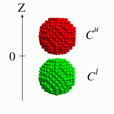
Figure 1: (Color online) A typical situation of our simulation of two colliding clusters. Each of them contains 682 “atoms” which are bound by the Lennard-Jones potential.

Table 1: Relation between numbers of layers and atoms.

Number of Layers	Number of Atoms
3	12
5	42
7	135
9	236
11	433
13	682
15	1055
17	1466

Henceforth, we label the upper and the lower clusters as $C^{u}$ and $C^{l}$, respectively. We assume that the interactive potential between the atom $k$ on the lower surface of $C^{u}$ and the atom $l$ on the upper surface of $C^{l}$ is given by

$$\varphi(r_{kl})=4\epsilon\left\{\left(\frac{\sigma}{r_{kl}}\right)^{12}-c\left(\frac{\sigma}{r_{kl}}\right)^{6}\right\},$$ (2)

where $r_{kl}$ is the distance between the surface atom $k$ and atom $l$. We introduce the cohesive parameter $c$ to characterize the attraction between the atoms of different clusters.awasthi

The procedure of our simulation is as follows. As the initial condition of simulation, the centers of mass of $C^{u}$ and $C^{l}$ are placed along the $z$-axis with the separation $\sigma_{c}$ between the surfaces of $C^{u}$ and $C^{l}$. The initial velocities of the “atoms” in both $C^{u}$ and $C^{l}$ obey Maxwell-Boltzmann distribution with the initial temperature $T$. The initial temperature is set to be $T=0.02\epsilon$ in our simulations. Sample average is taken over different sets of initial velocities governed by the Maxwell-Boltzmann velocity distribution for “atoms”.

To equilibrate the clusters, we adopt the velocity scaling method woodcock ; nose and perform $2000$ steps simulation for the relaxation to a local equilibrium state. Here let us check the equilibration of the total energy in the initial relaxation process. Figure 2(a) is the time evolution of the kinetic temperature of $C^{u}$, where $\bar{T}$ denotes the scaled temperature by the unit $\epsilon$. This figure shows the convergence of temperature to the desired temperature $T=0.02\epsilon$. On the other hand, Fig.2(b) is the probability density distribution of speed of “atoms” in $C^{u}$ when the equilibration process is over, where $\bar{v}$ denotes the scaled velocity for “atom” by the unit $\sqrt{\epsilon/m}$. The solid curve in Fig.2(b) shows the probability density distribution of speed $v_{i}$ of “atoms” indexed by $i$ in equilibrium,

$$\chi(v_{i})=4\pi\left(\frac{m}{2\pi kT}\right)^{3/2}v_{i}^{2}\exp\left(-\frac{m}{2kT}v_{i}^{2}\right),$$ (3)

with $T=0.02\epsilon$. This agreement shows that the upper cluster $C^{u}$ is equilibrated during the equilibration process.

Figure 2: (a) Relaxation of kinetic temperature and (b) distribution of speed of atoms after equilibration process. $\bar{T}$ and $\bar{v}$ are temperature and speed of “atom” scaled by units $\epsilon$ and $\sqrt{\epsilon/m}$, respectively.

After the equilibration, we give translational velocities to $C^{u}$ and $C^{l}$ to make them collide against each other. The relative speed of impact ranges from $V=0.02\sqrt{\epsilon/m}$ to $V=0.6\sqrt{\epsilon/m}$. Here, the characteristic speed is the thermal velocity for one “atom” $\sqrt{T/m}$, where $m$ is the mass of each “atom”. This situation might correspond to the sputtering process or collisions of interstellar dusts or atmospheric dusts. Although it is not easy to control the velocity of colliding clusters in real nanoscale experiments, the effects of thermal fluctuation to the center of mass of each cluster might be negligible if clusters are flying in vacuum.

Numerical integration of the equation of motion for each atom is carried out by the second order symplectic integrator with the time step $dt=1.0\times 10^{-2}\sigma/\sqrt{\epsilon/m}$. To reduce computational costs, we introduce the cut-off length $\sigma_{c}=2.5\sigma$ of the Lennard-Jones interaction, which sometimes affects the energy conservation of a system although the Hamiltonian of the system is conserved. We have checked that the rate of energy conservation, $|E(t)-E_{0}|/|E_{0}|$, is kept within $10^{-5}$ with the cutoff length $\sigma_{c}=2.5\sigma$, where $E_{0}$ is the initial energy of the system and $E(t)$ is the energy at time $t$. In general, the value between $3\sigma\leq\sigma_{c}\leq 4\sigma$ is used for the energy conservation about $|E(t)-E_{0}|/|E_{0}|\sim 10^{-5}$.

We let the angle around $z-$axis, $\theta_{z}$, be $\theta_{z}=0$ when the two clusters are located mirror-symmetrically with respect to $z=0$. In most of our simulation, we set $\theta_{z}$ at $\theta_{z}=0$ as the initial condition. The dependency on $\theta_{z}$ will be shown in the next section.

III Results of our simulation

III.1 Relation between impact speed and restitution coefficient

Figures 3 (a) and (b) display, respectively, the magnified sequential plots of colliding clusters for a purely repulsive collision and a cohesive collision when the initial temperature and the impact speed are $T=0.02\epsilon$ and $V=0.3\sqrt{\epsilon/m}$. From Fig. 3, we confirm that the contact duration for the cohesive collision is longer than that of the repulsive collision.awasthi During the restitution, we also observe the elongation of the clusters along the $z$-axis in cohesive collisions, while we can not observe such a phenomenon in repulsive collisions. In both cases, the rotation of clusters is slightly excited after a collision.

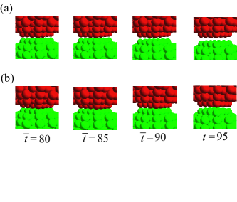
Figure 3: (Color online) Sequential plot of collisions for (a) c=0.0 and (b) c=0.2 at $\bar{t}=80$, $85$, $90$, and $95$, where $\bar{t}$ is time scaled by unit $\sigma/\sqrt{\epsilon/m}$.

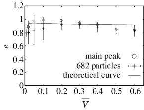
Figure 4: Relationship between colliding speed and restitution coefficient for $c=0.2$. $\bar{V}$ is relative colliding speed scaled by unit $\sqrt{\epsilon/m}$.

We firstly investigate the relation between the colliding speed and the restitution coefficient for a weak attractive case ($c=0.2$). The cross points in Fig. 4 show the relationship between the relative speed of impact scaled by the unit $\sqrt{\epsilon/m}$, $\bar{V}\equiv V/\sqrt{\epsilon/m}$, and the restitution coefficient $e$. Sample average is taken over 100 different initial conditions for each speed and the error bar shows the standard deviation. From Fig. 4 we find that the restitution coefficient has a peak around the colliding speed $V=0.2\sqrt{\epsilon/m}$, which is attributed to the reduction of $e$ caused by the attractive force in the lower impact speed. This tendency can also be observed in cohesive collisions of macroscopic bodies. brilliantov07 ; louge2008

The solid line in Fig. 4 represents the theoretical prediction of cohesive collisions between viscoelastic spheres.brilliantov07 Here, we briefly summarize the theory of cohesive collisions in Ref.brilliantov07 . Let us consider a head-on collision between elastic spheres of radii $R_{1}$ and $R_{2}$, each of which has mass of $M_{1}$ and $M_{2}$, respectively. The basic idea of their theory is to solve the time evolution equation of the deformation $\xi(t)$ of the colliding spheres:

$$\mu\ddot{\xi}(t)+F(\xi(t))=0,$$ (4)

$$\xi(0)=0,\hskip 8.53581pt\dot{\xi}(0)=V,$$

where $\mu$ is the reduced mass $\mu=(1/M_{1}+1/M_{2})^{-1}$. $\xi(t)$ is described as the function of the radius of contact area $a$ as

$$\xi(a)=\frac{a^{2}}{R_{eff}}-\displaystyle\sqrt{\frac{8\pi\gamma Da}{3}}\hskip 8.53581pt\text{with}\hskip 8.53581ptR_{eff}=\left(\frac{1}{R_{1}}+\frac{1}{R_{2}}\right)^{-1},$$ (5)

so that Eqs.(4) are rewritten as

$$\mu\ddot{a}+\mu\frac{\xi^{{}^{\prime\prime}}(a)}{\xi^{{}^{\prime}}(a)}\dot{a}^{2}+\frac{F(a)}{\xi^{{}^{\prime}}(a)}=0,$$ (6)

$$a(0)=a_{init},\hskip 8.53581pt\dot{a}(0)=V\left(\frac{d\xi}{da}|_{a_{init}}\right)^{-1},$$ (7)

where the prime denotes the differentiation with respect to $a$. We adopt $a_{init}=(8\pi D\gamma R_{eff}^{2}/3)^{1/3}$ which is the contact radius of the bottom plane of the upper cluster with $\gamma\simeq 0.104\epsilon/\sigma^{2}$ estimated from the calculation of the attractive interaction between two clusters (see Appendix A ). We also estimate $D$ as $D=3.28\times 10^{-3}\sigma^{3}/\epsilon$ from Young’s modulus $Y=454\epsilon\sigma^{-3}$ and Poisson’s ratio $\nu=7.74\times 10^{-2}$ which are obtained from another simulation. ptps

They assume that the force $F(a)$ between cohesive spheres comprises three kinds of forces: elastic force $F_{H}(a)$ characterized by Hertzian contact theoryhertz ; landau , dissipative force $F_{dis}(a)$kuwabara , and cohesive Boussinesq force $F_{B}(a)$ derived from JKR theory.jkr Thus, the total force can be expressed by

$$F(a)=F_{H}(a)-F_{B}(a)+F_{dis}(a).$$ (8)

Here, the sum of the elastic force and the Boussinesq force is given by

$$F_{H}(a)-F_{B}(a)=\frac{a^{2}}{R_{eff}}-\displaystyle\sqrt{\frac{6\pi\gamma}{D}}a^{3/2}$$ (9)

with the surface tension $\gamma$ and $D=(3/4)\{(1-\nu_{1}^{2})/2Y_{1}+(1-\nu_{2}^{2})/2Y_{2}\}$ with Poisson’s ratio $\nu_{i}$ and Young’s modulus $Y_{i}$ for the cluster $i=1,2$. Following the idea in Ref.brilliantov07 , we assume that the dissipative force is given by

$$F_{dis}(a)=A\dot{a}\frac{\partial}{\partial a}(F_{H}(a)-F_{B}(a)),$$ (10)

where $A$ is a fitting parameter.

We solve Eq.(6) with the initial speed $V$ ranging from $0.01(\epsilon/m)^{1/2}$ to $0.6(\epsilon/m)^{1/2}$ by the use of the fourth order Runge-Kutta method to obtain the rebound speed which is the speed when the contact radius $a$ becomes less than $a_{sep}\equiv\left(3\pi D\gamma R^{2}_{eff}/2\right)^{1/3}$.brilliantov07 From the rebound speed for each impact speed, we obtain the relationship between the restitution coefficient and the impact speed. In Fig. 4, we use $A=0.1\sigma\sqrt{m/\epsilon}$ to draw the theoretical curve. In $V<0.2\sqrt{\epsilon/m}$, the discrepancy between our numerical results (cross points) and the theoretical result is large, which may be attributed to the rotational rebounds of clusters after collisions. On the other hand, the theoretical curve reproduces the results of simulation which excludes rotation of clusters (open circles) as will be explained later.

Here, let us briefly comment on the dependence of the relative angle $\theta_{z}$ on the numerical results. We have checked $\theta_{z}$ dependence of the restitution for purely repulsive collisions, i.e. $c=0.0$ at $T=0.02\epsilon$. Figure 5 shows the relationship between impact speeds and restitution coefficients for $\theta_{z}=0,\pi/6,\pi/3,\hskip 2.84526pt\text{and}\hskip 2.84526pt\pi/2$. This figure indicates that the relation between the impact speed and the restitution coefficient is not largely affected by the initial orientation, although the orientation around other axes may affect the relation. Thus, we will analyse only the results obtained with the fixed initial orientation $\theta_{z}=0$.

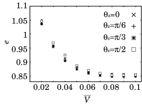
Figure 5: Relation between relative colliding speed and restitution coefficient for different initial angles for $c=0.0$ and $T=0.02\epsilon$.

III.2 Distribution of restitution coefficient

In this subsection, we investigate the frequency distributions of restitution coefficients for purely repulsive collisions and cohesive collisions, respectively. Figure 6(a) shows the histogram of the restitution coefficient for purely repulsive collisions ($c=0.0$). To obtain this result, we take $5000$ samples at the fixed impact speed $V=0.02\sqrt{\epsilon/m}$. From Fig. 6(a), the frequency distribution can be approximated by the Gaussian (solid line) for purely repulsive collisions.

On the other hand, Fig. 6(b) shows the frequency distribution of the restitution coefficient for cohesive collisions ($c=0.2$). To obtain this result, we take $995$ samples at the fixed impact speed $V=0.1\sqrt{\epsilon/m}$. In Fig. 6(b), we find the existence of the two peaks around $e=0.448$ and $e=0.656$, respectively, except for the main peak around $e=0.982$. From the check of simulation movies, the collisions around these small peaks are produced by rotations after the collisions, while the most of bounces are not associated with rotations in the vicinity of the main peak around $e=0.982$. It is reasonable that the excitation of macroscopic rotation lowers the restitution coefficient.

Figure 6: Histograms of restitution coefficients for (a) $c=0.0$, $V=0.02\sqrt{\epsilon/m}$, and (b) $c=0.2$, $V=0.1\sqrt{\epsilon/m}$. The solid line in (a) is the Gaussian fitting of the data.

Here, let us make another comparison of our simulation result with the theoretical curve drawn in Fig.4. The open circles in Fig.4 are the mean values obtained by the data around the main peak for each impact speed to remove the effects of rotational bounces. It is obvious that the theory has a better fitting curve of the data when we remove rotational bounces.

We shall comment on the fitting function of the main peak. Figure 6(b) shows that the distribution around the main peak has an asymmetric profile, so that the Gaussian function may fail to fit the tail parts of the main peak.

Figure 7: Semi-log plot of the main peak in Fig.6(b). The solid lines are the double exponential functions to fit the data.

Figure 7 shows the semi-log plot of the simulation data around the main peak, where $F(e)$ is the frequency of $e$. The reasonable fitting curves are represented by the solid lines, where $\ln F(e)=(19.6\pm 1.9)e+(-14.7\pm 1.8)$ for $e<0.982$ and $\ln F(e)=(-127\pm 28)e+(130\pm 28)$ for $e>0.982$, respectively. Thus, the distribution of restitution coefficients can be approximated by a combination of the double-exponential functions when the rotation is not excited after impacts. A similar tendency has also been observed in a recent experiment and a recent simulation of macroscopic collisions. poeschel2008

III.3 Phase diagram of restitution coefficient

As discussed in the previous subsection, some samples of the restitution coefficient exceeds unity even for cohesive collisions. We can guess that most of colliding clusters coalesce when we use the collisional model with $c=1$. Thus, it is important to know what process actually occurs after a collision when the impact speed or the cohesive parameter $c$ is given. In this subsection, we investigate the emergence probability of four modes of the collisions (i) coalescence, (ii) bouncing, (iii) normal collision with $e<1$, and (iv) anomalous collision with $e>1$. The coalescence (i) and the bouncing (ii) can take place only when the attractive interaction between the colliding clusters exists. Indeed, the bouncing occurs as the result of trapping by the potential well, if the rebound speed is not large enough. awasthi06

Figure 8 (a) shows the phase diagram which is obtained under the fixed colliding speed $V=0.02\sqrt{\epsilon/m}$, where $P$ represents the probability to observe each mode. This phase diagram shows that the regions for the modes (iii) and (iv) decrease with the increase of $c$. In the strong attractive case, $c>0.6$, we cannot observe rebound modes (ii), (iii), and (iv). Here, we find that the anomalous impact can be observed for cohesive collisions with $c<0.4$.

We also categorize collisions into four modes as a function of the impact speed under the fixed cohesive parameter $c=0.2$ (Fig.8 (b)). Here, we find that the probability to emerge the modes (i) and (ii) decreases with the increase of the impact speed. In addition, the anomalous impact can be observed within the range of impact speed $0.02\leq V/(\epsilon/m)^{1/2}\leq 0.1$. It is interesting that Fig.8(b) for $V<0.04\sqrt{\epsilon/m}$ is almost the mirror symmetric one of Fig.8(a) for $c<0.2$, which suggests that the cohesive parameter plays a role of the impact speed.

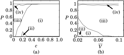
Figure 8: Probability diagrams classified by four collision modes with fixing (a) $V=0.02\sqrt{\epsilon/m}$ and (b) $c=0.2$, respectively.

Here let us reproduce the results of our simulation qualitatively by a phenomenology. Purely repulsive collisions, as we expect from Fig. 6(a), the probability density distribution of rebound speed $V^{{}^{\prime}}$ can be approximated by a Gaussian function

$$p(V^{{}^{\prime}})=\frac{1}{\sqrt{\pi\alpha}}\exp\left[-\frac{(V^{{}^{\prime}}-V_{m})^{2}}{\alpha}\right].$$ (11)

Thus, for given impact speed $V$, we can use Eq.(11) where $V_{m}$ and $\alpha$ in Eq.( 11) are fitting parameters. Then, we calculate the probability to exceed the escape speed $V^{*}$ barger from the attractive potential field $\Phi(r)\equiv-4\epsilon c(r/\sigma)^{-6}$ under the given $V^{\prime}$. Here the escape speed $V^{*}$ of a rebounded cluster may be given by

$$V^{*}/\sqrt{\epsilon/m}=\sqrt{2\Phi(x^{*}/\sigma)/\sigma\mu},$$ (12)

where $x^{*}=(2/c)^{1/6}\sigma$ at which the potential takes the minimum value. For example, the escape speed becomes $V^{*}=0.015(\epsilon/m)^{1/2}$ in the case of $c=0.2$.

Thus, from integrating the probability densities of $V^{{}^{\prime}}$, the probabilities to observe modes (i), (iii), and (iv) are respectively given by

$$P^{(\rm{i})} = \int_{-\infty}^{V^{*}}p(V^{{}^{\prime}})dV^{{}^{\prime}}=\frac{1}{2}\left\{1-{\rm erf}\left(\frac{V_{m}-V^{*}}{\sqrt{\alpha}}\right)\right\},$$ (13)

$$P^{(\rm{iii})} = \int_{V^{*}}^{V}p(V^{{}^{\prime}})dV^{{}^{\prime}}=\frac{1}{2}\left\{1-{\rm erf}\left(\frac{V_{m}-V}{\sqrt{\alpha}}\right)\right\}-P^{\rm{(i)}},$$ (14)

$$P^{\rm{(iv)}} = \int_{V}^{\infty}p(V^{{}^{\prime}})dV^{{}^{\prime}}=1-P^{\rm{(i)}}-P^{\rm{(iii)}},$$ (15)

where ${\rm erf}(x)$ is the error function ${\rm erf}(x)\equiv\int_{-\infty}^{x}\exp(-t^{2})dt$. Here we ignore the distinction between the mode (i) and the mode (ii), because the most of bouncing clusters eventually coalesce after some numbers of collisions.

Figure 9: Probability diagrams from our theoretical argument for (a) $V=0.02\sqrt{\epsilon/m}$ and (b) $c=0.2$.

Figures 9 (a) and (b) show the probability diagrams obtained from Eqs. (13), (14), and (15). To draw Fig.9(b), we adopt $V^{*}=0.018\sqrt{\epsilon/m}$ which is slightly larger than the calculated value $V^{*}=0.015\sqrt{\epsilon/m}$ by Eq.(12) for $c=0.2$. Our phenomenology qualitatively reproduces the diagrams obtained by the simulation as in Figs.8 (a) and (b), although there are some quantitative differences between the simulation and the phenomenology. Indeed, the probability to appear the mode (iv) in the phenomenology decreases with the increase of $V\sqrt{\epsilon/m}$ as in Fig.9 (b), but this tendency cannot be observed in the simulation in Fig.8 (b).

IV Discussion

Let us discuss our results. We, mainly, discuss how the restitution coefficient depends on the cluster size in this section. Figure 10 shows the relationship between the relative colliding speed of clusters and the restitution coefficient with different sizes of 236 atoms ($\rm{C}_{236}$), 433 atoms ($\rm{C}_{433}$), and 682 atoms ($\rm{C}_{682}$), respectively, where we use the data obtained by the fixed parameters $c=0.2$ and $T=0.02\epsilon$. As can be seen in Fig. 10, the restitution coefficients satisfies the scaling in which $e(R/\sigma)^{0.317}$ is a universal function of the impact speed, where $R$ is the radius of each cluster.

Figure 10: Relation between colliding speed and restitution coefficient for clusters $\rm{C}_{236}$, $\rm{C}_{433}$, and $\rm{C}_{682}$. The restitution coefficients are scaled by $R^{0.317}$, where $R$ is the radius of each cluster.

To obtain the scaling exponent, we first calculate the standard deviation for each rebound speed under the fixed value of the exponent. Next, we search the value of the exponent such that the maximum value of the standard deviations has a minimum value. To draw the solid curve in Fig.10, we solve eq.(6) with the fitting parameter $A=0.1\sigma\sqrt{m/\epsilon}$ for $\rm{C}_{682}$ with the aid of its radius $R_{eff}=3.23\sigma$. This is interesting finding from our simulation which has not been predicted by the quasistatic theory of cohesive collisions for macroscopic bodies.brilliantov07

From a simple phenomenology, we can understand that the restitution coefficient depends on the radius. However, the phenomenology predicts that $e(R/\sigma)^{1/2}$ satisfies a scaling relation (see Appendix B). The discrepancy between the phenomenology and the numerical observation indicates that our over-simplified theory is insufficient. We will need a more sophisticated theory to explain the exponent.

We also simulate collisions between larger clusters than $\rm{C}_{682}$ by the use of $\rm{C}_{1055}$ and $\rm{C}_{1466}$. Figure 11 (a) is the relationship between the impact speed and the restitution coefficients in the case of $c=0.0$ under the initial temperature $T=0.02\epsilon$. The squares, plus points, and circles show the averaged data of $\rm{C}_{682}$, $\rm{C}_{1055}$, $\rm{C}_{1466}$, respectively. We take $10$ samples for both $\rm{C}_{1055}$ and $\rm{C}_{1466}$ while $100$ samples for $\rm{C}_{682}$. Here we do not find any systematic relationship between the impact speed and the restitution coefficients in the cases of $\rm{C}_{1055}$ and $\rm{C}_{1466}$. This can be attributed to the surface instability of the clusters arising from the weak attraction between “atoms”.

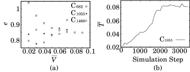
Figure 11: (a) Relation between impact speed and restitution coefficient in cases of $\rm{C}_{682}$, $\rm{C}_{1055}$, and $\rm{C}_{1466}$. (b) Time evolution of internal temperature of cluster $\rm{C}_{1055}$ in its free flight after initial equilibration to $T=0.02\epsilon$.

It is known that the instability of the spherical shape and the plastic deformation in a cluster cause the increase of the internal temperature of the cluster.awasthi ; suri We numerically performed free flights of cluster by the use of $\rm{C}_{1055}$ to check the time evolution of the internal temperature of the cluster. Figure 11(b) shows the time evolution of the temperature inside the cluster $\rm{C}_{1055}$ after giving the translational speed $V=0.07\sqrt{\epsilon/m}$ and the initial temperature $T=0.02\epsilon$. Here we find the temperature increase during the free flight up to around $T=0.08\epsilon$. Thus, we conclude that the maximum number of “atom” to reproduce the theory of cohesive collision is $682$ in our system.

We try to estimate the critical radius theoretically on the basis of the argument of capillary instability of elastic droplets (see Appendix C),landau2 but our over-simplified theory predicts that any elastic surface of spheres are unstable under the gravity. We should note that this calculation is based on theory of elasticity with zero shear modulus (Poisson’s ratio is equal to -1). The calculation suggests that (i) we may not use theory of elasticity or (ii) zero shear modulus is unrealistic. We will, at least, need to discuss the capillary instability under the full set of elastic equations. From these arguments, we regard $\rm{C}_{682}$ as the maximum size to reproduce the quasi-static theory of cohesive collisions in our modelling.

Although our simulation mimics impact phenomena of small systems subject to large thermal fluctuations, we should address that our model with small $c$ may not be adequate for the description of many of realistic collisions of nanoclusters, where the cohesive interaction between clusters often prohibits the rebound in the low-speed impact. Namely, the corresponding value of the cohesive parameter is large in many of actual situations. However, nanoscale impacts can be realized experimentally by the using the surface coated nanoclusters. For example, it has been demonstrated that hydrogen coated Si nanoparticles exhibit the weak attraction by H atoms on the surface.suri ; hawa We believe that our model captures the essence of such a system. For realistic simulations, we may need to carry out another simulation of the collision of H-passivated Si clusters by introducing suitable empirical potentials. As an additional remark, we should indicate that it is difficult to control the colliding speed and the initial rotation of the cluster in actual situations because the macroscopic motion of one cluster is also affected by thermal fluctuations.

V Conclusion

In conclusion, we have performed molecular dynamics simulations to investigate the behaviors of colliding clusters and the relationship between the restitution coefficient and the impact speed. The results of our simulations have revealed that some aspects of the relationship can be understood by the quasi-static theory for cohesive collisions.brilliantov07 In addition, we have drawn the phase diagram of the restitution coefficient in terms of the impact speed and the cohesive parameter and explained them by a simple phenomenology. To clarify the mechanism of the emergence of the anomalous impact, it may need further investigation about the internal state of clusters during collision such as stress and modal analyses.

Appendix A Calculation of surface tension

In this appendix we explain how we calculate the surface tension $\gamma$ used to draw the theoretical curve in Fig. 4.surf Let us assume that two identical clusters are in plane-to-plane contact with each other. When those clusters are located by the separation $d$, the surface energy per unit area $W$ is given bysurf

$$W\simeq\frac{B}{12\pi d_{0}^{2}}\left(1-\frac{d_{0}^{2}}{d^{2}}\right),$$ (16)

where $B$ is the Hamaker constant $B\equiv 4\pi^{2}\epsilon c\sigma^{6}\rho^{2}$ with the cohesive parameter $c$ and the number density $\rho$ of each cluster. In our model, we use the number density becomes $\rho=0.4\sigma^{-3}$, and $d_{0}\simeq 0.4\sigma$.

The surface tension $\gamma$ is equal to the energy per unit area to separate the two contacting plane to infinity. Thus, we obtain $\gamma$ as

$$\gamma=\frac{B}{24\pi d_{0}^{2}}\simeq 0.0261\times\frac{4\epsilon}{\sigma^{2}}=0.1044\frac{\epsilon}{\sigma^{2}}.$$ (17)

Appendix B Dependence of $e$ on $R$

Let us derive a scaling relation between the restitution coefficient and the radius of cluster. Our assumption is that (i) the energy dissipation during a collision is originated from the sum of of the viscous force and the Boussinesq force, (ii) energy dissipation from the Boussinesq force is approximately given by the work during the detachment process of two coalesced clusters.

Let us first estimate the energy dissipation caused by the surface tension. A pair of colliding clusters is partially coalesced as shown in Figure 12, where we assume that the deformation of two spheres are negligible, and contacted state can be characterized by a simple cut of the deformed region. Let $\theta$ be the angle around the center of the upper sphere ranging from $-\theta_{0}$ to $\theta_{0}$ under the assumption a small $\theta_{0}$.

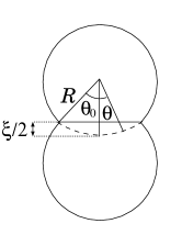
Figure 12: Schematic figure of contacting identical spheres.

From this figure, the surface area of a cut hemi-sphere is approximately given by $\pi R^{2}\theta^{2}_{0}=\pi R\xi$ with the deformation $\xi\simeq\theta_{0}^{2}R$. Thus, the work needed to pull off two spheres is

$$W_{\gamma}\simeq 2\pi\gamma R\xi_{max}\sim\left(\frac{\rho_{0}}{Y}\right)^{2/5}R^{2}V^{4/5},$$ (18)

where we use the estimation $\xi_{max}\propto(\rho_{0}R^{3}/Y\sqrt{R})^{2/5}V^{4/5}\sim(\rho_{0}/Y)^{2/5}RV^{4/5}$ on the basis of the theory of elasticity, where $\rho_{0}$ is the density.landau

On the other hand, the energy dissipation of repulsive spheres is given bykuwabara

$$E_{loss}^{dis}\propto\rho_{0}^{3/5}\tau Y^{2/5}R^{2}V^{11/5},$$ (19)

where $\tau$ is time scale of the dissipation. From the combination of two terms in eqs. (18) and (19), we obtain the expression of the total energy loss during a collision

$$E_{loss}=E_{loss}^{dis}-W_{\gamma}\sim R^{2}(c_{1}V^{11/5}-c_{2}V^{4/5}),$$ (20)

where $c_{1}\simeq\rho_{0}^{3/5}\tau Y^{2/5}$ and $c_{2}\simeq(\rho_{0}/Y)^{2/5}$. Since Eq.(20) should be balanced with $\rho_{0}R^{3}V^{2}(1-e^{2})$, we obtain

$$R(1-e^{2})\sim\frac{1}{\rho_{0}}(c_{1}V^{1/5}-c_{2}V^{-6/5}).$$ (21)

Thus, our phenomenology suggests that $R^{1/2}e$ is independent of the radius of the colliding spheres.

Appendix C Instability of an elastic droplet

In this appendix we investigate the instability of the surface profile of clusters on the assumption that the internal modes of the cluster are expressed by those of an isotropic elastic sphere. When the shear stress can be ignored, the stress tensor $\sigma_{ij}$ can be written as

$$\sigma_{ij}=K\nabla\cdot{\bf u}\delta_{ij},$$ (22)

where $K$ is the bulk modulus, $\delta_{ij}$ is Kronecker delta, and ${\bf u}$ is the strain. Thus, the equation of motion in the bulk becomes

$$\rho\ddot{\bf u}=\nabla(K\nabla\cdot{\bf u})=-\nabla p,$$ (23)

where $\rho$ is the density and $p\equiv-K\nabla\cdot{\bf u}$ is the effective pressure. Thus, the problem can be mapped onto a problem of perfect fluid. Thus, the dispersion relation is linearized equation $R(\theta,\phi,t)=R_{0}+\zeta(\theta,\phi,t)$ can be written as

$$\omega^{2}_{l}=\frac{\gamma l(l-1)(l+2)}{\rho R^{3}_{0}},$$ (24)

as in the case of a liquid dropletlandau2 , where $l$ is the index of Legendre polynomial.

When we introduce the gravity in this perfect fluid model, the scalar potential $\Phi$ defined by ${\bf v}=\nabla\Phi$ satisfies

$$\partial_{t}\Phi+P+\frac{1}{2}v^{2}+gz=f(t),$$ (25)

where where $\partial_{t}$ is the time derivative, $P=\int dp/\rho(p)$, and $f(t)$ is an arbitrary function of time, $g$ and $z$ are the gravitational acceleration and the relative vertical position from the center of mass of the sphere. Choosing $f(t)$ satisfying $f(t)=p_{0}+\gamma\left(\frac{1}{R_{1}}+\frac{1}{R_{2}}\right)$ with the surface tension $\gamma$, curvatures $R_{1}$ and $R_{2}$, Eq. (25) can be rewritten as

$$\rho\ddot{\Phi}=\frac{\gamma}{R^{2}_{0}}\left\{2\frac{\partial\Phi}{\partial r}-\Lambda(\theta,\phi)\frac{\partial\Phi}{\partial r}\right\}+\rho g\cos\theta\frac{\partial\Phi}{\partial r}.$$ (26)

where $\Lambda(\theta,\phi)=-\left\{\frac{1}{\sin\theta}\frac{\partial}{\partial\theta}\left(\sin\theta\frac{\partial}{\partial\theta}\right)+\frac{1}{\sin^{2}\theta}\frac{\partial^{2}}{\partial\phi^{2}}\right\}$. To derive Eq. (26) we have used $\dot{\Psi}=\Phi$, ${\bf v}=\dot{\bf u}=\nabla\Psi$, and $\dot{\zeta}=v_{r}=\partial\Phi/\partial r$ at $r=R_{0}$.

By using the expansion $\Phi$ in terms of $r^{l}$ and the spherical harmonic function $Y_{l,m}(\theta,\phi)$, we may obtain

$$\omega_{l,m}^{2}=\frac{\gamma}{\rho R_{0}^{3}}l(l-1)(l+2)-\frac{lg}{R_{0}}\left\{\sqrt{\frac{(l-m)(l+m)}{(2l-1)(2l+1)}}+\sqrt{\frac{(l-m+1)(l+m+1)}{(2l+1)(2l+3)}}\right\},$$ (27)

where we have used the formula

$$\cos\theta Y_{lm}=\displaystyle\sqrt{\frac{(l-m+1)(l+m+1)}{(2l+1)(2l+3)}}Y_{l+1,m}\\ +\displaystyle\sqrt{\frac{(l-m)(l+m)}{(2l-1)(2l+1)}}Y_{l-1,m}.$$ (28)

Therefore, $\omega_{n,l,m}$ becomes complex, if the radius exceeds the critical radius

$$R_{0,c}^{(l,m)}=\left[\frac{\gamma(l-1)(l+2)}{\rho g\left\{\displaystyle\sqrt{\frac{(l-m)(l+m)}{(2l-1)(2l+1)}}+\displaystyle\sqrt{\frac{(l-m+1)(l+m+1)}{(2l+1)(2l+3)}}\right\}}\right]^{1/2}.$$ (29)

Equation (29) implies that the mode with $l=1$ is always unstable for the perturbation. Thus, we conclude that an accelerated elastic sphere is unstable, which is similar to the instability of a raindrop of the perfect fluid because the neutral mode $l=1$ does not have any recovering force.

References

- (1) J. H. Vincent, Proc. Camb. Phil. Soc. 10, 332 (1900).
- (2) C. V. Raman, Phys. Rev. 12, 442 (1918).
- (3) W. Goldsmith, Impact: the theory and physical behavior of colliding solids (E. Arnold, London, 1960).
- (4) W. J. Stronge, Impact Mechanics (Cambridge Univ. Press, Cambridge, 2000).
- (5) F. G. Bridges, A. Hatzes, and D. N. C. Lin, Nature 309, 333 (1984).
- (6) G. Kuwabara and K. Kono, Jpn. J. Appl. Phys. 26, 1230 (1987).
- (7) W. A. M. Morgado and I. Oppenheim, Phys. Rev. E 55, 1940 (1997).
- (8) N. V. Brilliantov, F. Spahn, J.-M. Hertzsch and T. Pöschel, Phys. Rev. E 53, 5382 (1996).
- (9) T. Schwager and T. Pöschel, Phys. Rev. E 57, 650 (1998).
- (10) R. Ramírez, T. Pöschel, N. V. Brilliantov, and T. Schwager, Phys. Rev. E 60, 4465 (1999).
- (11) K. L. Johnson, Contact Mechanics (1st ed.) (Cambridge Univ. Press, Cambridge, 1985).
- (12) F. Gerl and A. Zippelius, Phys. Rev. E 59, 2361 (1999).
- (13) H. Hayakawa and H. Kuninaka , Chem. Eng. Sci. 57, 239 (2002).
- (14) M. Y. Louge and M. E. Adams, Phys. Rev. E 65, 021303 (2002).
- (15) H. Kuninaka and H. Hayakawa, Phys. Rev. Lett. 93, 154301 (2004); see also Phys. Rev. Focus 14, story 14 (2004).
- (16) J. Calsamiglia, S. W. Kennedy, A. Chatterjee, A. L. Ruina, and J. T. Jenkins, J. Appl. Mech. 66, 146 (1999).
- (17) H. Hertz, J. Reine Angew. Math. 92, 156 (1882).
- (18) L. D. Landau and E. M. Lifshitz, Theory of Elasticity (3rd English ed.) (Butterworth-Heinemann, Oxford, 1986).
- (19) H. Kuninaka and H. Hayakawa, J. Phys. Soc. Jpn. 75, 074001 (2006).
- (20) J. Tomas, Chem. Eng. Sci. 62, 1997 (2007); R. Tykhoniuk, J. Tomas, S. Luding, M. Kappl, L. Heim, and H-J. Butt, ibid. 62, 2843 (2007); J. Tomas, ibid. 62, 5925 (2007).
- (21) J. N. Israelachvili, Intermolecular and Surface Forces (2nd ed.) (Academic Press, London, 1992).
- (22) A. Castellanos, Adv. Phys. 54, 263 (2005).
- (23) N. V. Brilliantov, N. Albers, F. Spahn, and T. Pöschel, Phys. Rev. E 76, 051302 (2007).
- (24) C. M. Sorace, M. Y. Louge, M. D. Crozier and V. H. C. Law, Mech. Res. Comm. (in press).
- (25) M. Rieth, Nano-Engineering in Science and Technology (World Scientific, New Jersey, 2003).
- (26) M. P. Allen and D. J. Tildesley, Computer Simulation of Liquids (Clarendon press, Oxford, 1987).
- (27) M. Kalweit and D. Drikakis, J. Compt. Theor. Nanoscience 1, 367 (2004).
- (28) M. Kalweit and D. Drikakis, Phys. Rev. B, 74, 235415 (2006) and references therein.
- (29) O. Knospe and R. Schmidt, Theory of atomic and molecular clusters, ed. by J. Jellinek, 111 (Springer, Berlin, 1999).
- (30) A. Tomsic, H. Schröder, K. L. Kompa K. L., and C. R. Gebhardt, J. Chem. Phys. 119, 6314 (2003).
- (31) W. Harbich, Metal Clusters at Surfaces, ed. by Karl-Heintz, Meiwes-Broer, p.p.107 (Springer, Berlin, 2000).
- (32) Y. Sakiyama, S. Takagi, and Y. Matsumoto, Phys. Fluids, 16, 1620 (2004).
- (33) A. Awasthi, S. C. Hendy, P. Zoontjens, S. A. Brown, and F. Natali, Phys. Rev. B, 76, 115437 (2007).
- (34) M. Suri and T. Dumitricǎ, Phys. Rev. B. 78, 081405(R) (2008).
- (35) T. Hawa and M.R. Zachariah, Phys. Rev. B. 71, 165434 (2005).
- (36) H. Kuninaka and H. Hayakawa, to appear in Prog. Theor. Phys. Suppl. (2009); arXiv:0707.0533v1.
- (37) H. Hayakawa and H. Kuninaka, in Proceedings of XXXVI Summer School Advanced Problems in Mechanics 2008 edited by D. A. Indeitsev and A. M. Krivtov (Russian Academy of Science, St. Petersburg 2008) pp. 306-317.
- (38) L. V. Woodcock, Chem. Phys. Lett. 10, 257 (1971).
- (39) S. Nosé, Prog. Theor. Phys. Suppl. 103, 1 (1991).
- (40) K. L. Johnson, K. Kendall, and A. D. Roberts, Proc. R. Soc. London, Ser. A 324, 301 (1971).
- (41) T. Pöschel, private communication.
- (42) A. Awasthi, S. C. Hendy, P. Zoontjens, S. A. Brown, Phys. Rev. Lett, 97, 186103 (2006).
- (43) V. D. Barger and M. G. Olsson, Classical Mechanics - A modern perspective (McGrow-Hill, NY, 1973).
- (44) L. D. Landau and E. M. Lifshitz, Fluid Mechanics (2nd English ed.) (Butterworth-Heinemann, Oxford, 1987).