Composite wormholes in vacuum Jordan-Brans-Dicke theory.

Sergey M.Kozyrev, Sergey V. Sushkov
1. Scientific center gravity wave studies ”Dulkyn”, Kazan, Russian Federation.

2. Department of General Relativity and Gravitation, Kazan State University, Kremlevskaya str. 18, Kazan 420008, Russia and Department of Mathematics, Tatar State University of Humanities and Education, Tatarstan str. 2, Kazan 420021, Russia

New classes composite vacuum wormhole solutions of Jordan-Brans-Dicke gravitation is presented and analysed. It is shown that such solution holds for both, a bridge between separated Schwarzschild and Brans Universes and for a bridge connecting two Schwarzschild asymptotically flat regions joined by Brans throat. We have also noticed that there are some new possible candidates for wormhole spacetimes.

1. Introduction

Lately there has been renewed interest in the scalar-tensor theories of gravitation. Important arena where these theories have found immense applications is the field of wormhole physics. Several classes of solutions in the scalar-tensor theories support wormhole geometry. The most prominent example of scalar-tensor theories is perhaps the Jordan-Brans-Dicke (JBD) [1], [2]. Now a day, predictions of JBD theory to be consistent not only with the weak field solar system tests but also with the recent cosmological observations.

JBD theory describes gravitation through a metric tensor g_μν and a massless scalar field $\phi$. In this theory, static wormhole solutions were found in vacuum, the source of gravity being the scalar field. Several static wormhole solutions in JBD theory have been widely investigated in the literature [3], [4]. It was shown that three of the four Brans classes of vacuum solutions admit a wormholelike spacetime for convenient choices of their parameters.

The Birkhoff’s theorem does not hold in the presence of JBD scalar field, hence some static JBD solutions seem possible in spherically symmetric vacuum case [5]. In this context, we recall the well known fact that the first exact solutions of JBD field equations in widespread Hilbert coordinates were obtained in parametric form by Heckmann [6], soon after Jordan proposed scalar-tensor theory. Apart from this, he showed that the Schwarzschild solution represent solution of JBD field equations, too.

In this work, we have borrowed from astrophysicists the idea of boson stars that is generated by a complex scalar field matching with a vacuum exterior solution. Furthermore, there is now a growing consensus that wormholes are in the same chain of stars and black holes. On the other hand, it is known that the JBD scalar field $\phi$ plays the role of classical exotic matter required for the construction of traversable Lorentzian wormholes [7].

This work is organized as follows. After giving a short account of the JBD theory and its static spherically symmetric solutions, we explore the wormhole nature of Brans solutions in section 2. In section 3 composite wormhole nature of the Brans solutions will be discussed by impose certain junction conditions. In section 4 we give some new possible candidates for wormhole spacetimes. Finally, conclusions are drawn in section 5.

2. Interior solution

Scalar-tensor theories are described by the following action in the Jordan frame is:

$$S = \int dx\sqrt{-g}(\phi R-\omega\left(\phi\right)g^{\mu\nu}\nabla_{\mu}\phi\nabla_{\nu}\phi-$$ (1)

$$\ \ \;\ \;\ \;\ \;\ \;\ \;\ \;\ \;\ \;\ \;\ \;\ -\lambda\left(\phi\right))+S_{m}.$$

Here, R is the Ricci scalar curvature with respect to the space-time metric g_μν and S_m denote action of matter fields. We use units in which gravitational constant G=1 and speed of light c=1. The dynamics of the scalar field $\phi$ depends on the functions $\omega$($\phi$) and $\lambda$($\phi$). It should be mentioned that the different choices of such functions give different scalar-tensor theories. We restrict our discussion to the JBD theory which characterized by the functions $\lambda$($\phi$) = 0 and $\omega$($\phi$) = $\omega$/$\phi$, where $\omega$ is a constant.

Variation of (1) with respect to g_μν and $\phi$ gives, respectively, the D-dimensional field equations:

$$R_{\mu\nu}-\frac{1}{2}Rg_{\mu\nu}=\frac{1}{\phi\ }T_{\mu\nu}^{M}+T_{\mu\nu}^{JBD},$$ (2)

where

$$T_{\mu\nu}^{JBD} = [\frac{\omega}{\phi^{2}}\left(\nabla_{\mu}\phi\nabla_{\nu}\phi-\frac{1}{2}g_{\mu\nu}\nabla_{\alpha}\phi\nabla^{\alpha}\phi\right)+$$ (3)

$$\ \ +\frac{1}{\phi}\left(\nabla_{\mu}\nabla_{\nu}\phi-g_{\mu\nu}\nabla_{\alpha}\nabla^{\alpha}\phi\right)].$$

and

$$\nabla_{\alpha}\nabla^{\alpha}\phi=\frac{T_{\lambda}^{M\ \lambda}}{3+2\omega},$$ (4)

and $T_{\lambda}^{M\ \lambda}$ is the energy momentum tensor of ordinary matter which obeys the conservation equation $T_{\mu\nu;\lambda}^{M\ }$ g^νλ= 0.

Consider spherically symmetric spacetime geometry. The most common form of line element of a spherically symmetric spacetime in comoving coordinates can be written as

$$ds^{2} = -g_{tt}\left(r,t\right)dt^{2}+g_{rr}\left(r,t\right)dr^{2}+$$ (5)

$$+\mathcal{\rho}^{2}\left(r,t\right)d\Omega^{2}.$$

where d$\Omega^{2}$ is the element of solid angle. Four classes of static JBD theory solutions were derived by Brans himself way back in 1962. The Brans class I solution (in isotropic coordinates with $g_{rr}=e^{2\lambda}$, $g_{tt}=e^{2\nu}$, $\rho^{2}=r^{2}g_{rr}$) is given by

$$\phi = \phi_{0}\left(\frac{1-\frac{B}{r}}{1+\frac{B}{r}}\right)^{\frac{C}{A}},$$ (6)

$$\lambda = \lambda_{0}+\ln\left[\left(1+\frac{B}{r}\right)^{2}\left(\frac{1-\frac{B}{r}}{1+\frac{B}{r}}\right)^{\frac{A-C-1}{A}}\right],$$

$$\nu = \nu_{0}+\ln\left[\left(\frac{1-\frac{B}{r}}{1+\frac{B}{r}}\right)^{\frac{1}{A}}\right],$$

where:

$$A=\sqrt{\left(C+1\right)^{2}-C\left(1-\frac{\omega\ C}{2}\right)},$$

In order to investigate whether a given solution represents a wormhole geometry, it is convenient to cast the metric into Morris-Thorne canonical form:

$$ds^{2}=-e^{2\chi\left(\stackrel{{\scriptstyle*}}{{R}}\right)}dt^{2}+\left[1-\frac{b\left(\stackrel{{\scriptstyle*}}{{R}}\right)}{\stackrel{{\scriptstyle*}}{{R}}}\right]^{-1}dr^{2}+$$

$$\ \ \ \ \ \ \ \ +\stackrel{{\scriptstyle*}}{{R}}^{2}d\Omega^{2},$$ (7)

where $\chi\left(\stackrel{{\scriptstyle*}}{{R}}\right)$ and b$\left(\stackrel{{\scriptstyle*}}{{R}}\right)$ are arbitrary functions of the radial coordinate, $\stackrel{{\scriptstyle*}}{{R}}$. $\chi\left(\stackrel{{\scriptstyle*}}{{R}}\right)$ is denoted as the redshift function, for it is related to the gravitational redshift; b$\left(\stackrel{{\scriptstyle*}}{{R}}\right)$ is called the form function, because as can be shown by embedding diagrams, it determines the shape of the wormhole [8]. The radial coordinate has a range that increases from a minimum value at $\stackrel{{\scriptstyle*}}{{R}}_{0}$, corresponding to the wormhole throat, to a, where the interior spacetime will be joined to an exterior vacuum solution. In the case of JBD theory the expressions for wormhole geometry can be easily obtained by connecting two Schwarzschild asymptotically flat regions joined by means of Brans throat. Moreover, one can use even not asymptotically flat JBD solution for a throat region. The Brans class I solution can be cast to the form (7) by defining a radial coordinate $\stackrel{{\scriptstyle*}}{{R}}$ which is related with r via the expression

$$\stackrel{{\scriptstyle*}}{{R}}=r\left(1+\frac{B}{r}\right)^{1+\frac{C+1}{A}}\left(1-\frac{B}{r}\right)^{1-\frac{C+1}{A}}$$ (8)

The functions $\chi\left(\stackrel{{\scriptstyle*}}{{R}}\right)$ and b$\left(\stackrel{{\scriptstyle*}}{{R}}\right)$ are the given by [3]

$$\chi\left(\stackrel{{\scriptstyle*}}{{R}}\right)=\frac{1}{A}\ln\left[\left(\frac{1-\frac{B}{r}}{1+\frac{B}{r}}\right)\right],$$ (9)

$$b\left(\stackrel{{\scriptstyle*}}{{R}}\right)=\stackrel{{\scriptstyle*}}{{R}}\left[\left(1-\frac{r^{2}\left(\stackrel{{\scriptstyle*}}{{R}}\right)-B^{2}-2r\left(\stackrel{{\scriptstyle*}}{{R}}\right)\frac{B\left(C+1\right)}{A}}{r^{2}\left(\stackrel{{\scriptstyle*}}{{R}}\right)-B^{2}}\right)^{2}\right]$$ (10)

The axially symmetric embedded surface $z=z\left(\stackrel{{\scriptstyle*}}{{R}}\right)$ shaping the wormhole’s spatial geometry is obtained from

$$\frac{dz}{d\stackrel{{\scriptstyle*}}{{R}}}=\pm\left[\frac{\stackrel{{\scriptstyle*}}{{R}}}{b\left(\stackrel{{\scriptstyle*}}{{R}}\right)}-1\right]^{-\frac{1}{2}}$$ (11)

By definition of wormhole at throat its embedded surface is vertical. The throat of the wormhole occurs at $\ \stackrel{{\scriptstyle*}}{{R}}=\stackrel{{\scriptstyle*}}{{R}}_{0}$ such that $\ b\left(\stackrel{{\scriptstyle*}}{{R}}_{0}\right)=\stackrel{{\scriptstyle*}}{{R}}_{0}$. This gives minimum allowed r - coordinate radii r${}_{0}^{\pm}$ as

$$r_{0}^{\pm}=\frac{B}{A}\left[C+1\pm\sqrt{\left(C+1\right)^{2}-A^{2}}\right]$$ (12)

According to pioneering Brans and Dicke work [2] to discuss the perihelion rotation of a planet requires a specifications of the arbitrary constants in solution (6) in such a way that this solution agrees in the weak - field limit as viewed by a distant observer. Hence comparing the expression for scalar field of Brans class I solution with weak - field solution we get [9]

$$C=-\frac{1}{\omega+2}$$ (13)

On the contrary, one can explain exterior region of JBD spherically symmetric configurations by the Schwarzschild metric. In this case we make the reasonable demand that this solution of scalar-tensor theory field equations lead to free estimates of arbitrary constants and lower limit of $\omega$. In this context, we recall the fact that the above conjecture can be easily adopted in other three classes of Brans solutions.

3. Junction conditions

Hawking’s theorem [10] in JBD states that the only spherically symmetric vacuum solution is static and given (up to coordinate freedom) by the Schwarzschild metric. Using the key assumption that the Brans class I solution physically acceptable we shall consider that the JBD scalar field is distributed from the throat to a radius a, where the solution is matched to an exterior Schwarzschild vacuum spacetime.

$$\phi=1,$$

$$\lambda=ln\left[\left(1+\frac{\mu}{r}\right)^{2}\right],$$ (14)

$$\nu=\ln\left(\frac{1-\frac{\mu}{r}}{1+\frac{\mu}{r}}\right),$$

In this case the boundary surface entails via the field equations a jump in second derivations of metric coefficient, but first derivatives remains continuous so can be used to match to the vacuum solution. Now in order to justify calling the geometry a wormhole we need an explicit definition for the constants in Brans I solution (6). We have five equations for five unknowns B, C, $\phi_{0}$ $\lambda_{0}$ $\nu_{0}$. Thus, from the junction conditions, the interior metric and scalar field parameters can be determined at the boundary surface in terms of the exterior metric and scalar field parameters $\mu$, $\phi$ = 1. Hence, Darmois-Israel junction conditions are fulfilled. The brief computation yields [11]:

$$\ B = a\sqrt{\frac{2a^{2}-2a\mu+\mu^{2}\left(2+\omega\right)}{-2a\mu+2\mu^{2}+a^{2}\left(2+\omega\right)}},\ \ \ \ \ \ \ \ \ \ \ \ \ \ \$$

$$\ C = \frac{2\left(a^{2}-a\mu+\mu^{2}\right)}{a\mu\ \omega},\ \ \ \ \ \ \ \ \ \ \ \ \ \ \ \ \ \ \ \ \ \ \ \ \ \ \ \ \ \ \ \$$

$$\lambda_{0} = \ln\left(\frac{\left(1-\frac{2B}{B+a}\right)^{\frac{2a^{2}+2\mu^{2}+a\mu\left(\omega-2\right)}{A\ a\mu\ \omega}}\left(a+\mu\right)^{2}}{a^{2}-B^{2}}\right),\ \ \ \ \ \ \ \ \$$

$$\nu_{0} = \ln\left(\frac{\left(1-\frac{2B}{B+a}\right)^{-\frac{1}{A\ }}\left(a-\mu\right)}{a+\mu}\right),\ \ \ \ \ \ \ \ \ \$$

$$\phi_{0} = \left(\frac{a+B}{a-B}\right)^{\frac{2\left(a^{2}+\mu^{2}-a\mu\right)}{A\ a\mu\ \omega}}.\ \ \ \ \ \ \ \ \ \ \ \ \ \ \ \ \ \ \ \ \$$

The spatial distribution of the JBD scalar field is restricted to the throat neighborhood, so that the dimensions of these wormholes are not arbitrarily large. The junction surface, r = a, is situated outside the event horizon, i.e., a$>\mu$, to avoid a black hole solution.

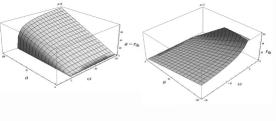
Figure 1: The surface represents the value of throat of the wormhole as a function of $\omega$ and junction radius a

Suppose we consider the Brans solution as a throat of wormhole. We were led to this model by considering a bridge between separated Schwarzschild and Brans Universes or a bridge connecting two Schwarzschild asymptotically flat regions.

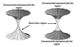
Figure 2: Two types of the composite wormholes. The visualization of the surface generated by the rotation of the embedded curve about the vertical z axis.

The same procedure can be easily adopted in other three classes of Brans solutions.

4. Other possible composite wormholes

Finally, we should mention yet another proposal related to wormholes. However, to our knowledge, exact complex scalar field (boson stars) and for vector-metric wormhole solutions are relatively scarce. The field equations of the vector-metric theory [12] are obtained by the similar variational method as the Einstein theory, and are given as following:

$$R_{\mu\nu}-\frac{1}{2}Rg_{\mu\nu}+\omega\stackrel{{\scriptstyle\left(\omega\right)}}{{\Theta}}_{\mu\nu}+\eta\stackrel{{\scriptstyle\left(\eta\right)}}{{\Theta}}_{\mu\nu}+$$

$$+\varepsilon\stackrel{{\scriptstyle\left(\varepsilon\right)}}{{\Theta}}_{\mu\nu}+\tau\stackrel{{\scriptstyle\left(\tau\right)}}{{\Theta}}_{\mu\nu}=8\pi T_{\mu\nu}^{M},$$ (15)

$$\varepsilon K_{;\nu}^{\mu\nu}+\frac{1}{2}\tau K_{;\nu}^{\mu\nu}-\frac{1}{2}\omega K^{\mu}R-\frac{1}{2}\eta K^{\nu}R_{\nu}^{\mu}=0.$$

where $\stackrel{{\scriptstyle\rightarrow}}{{K}}$ vector field and $\omega,\eta,\varepsilon,\tau$ free parameters. Indeed, for the absence of vector potential in empty space equations (15) become identical to field equation of Einstein theory. In a case of static spherically symmetric spacetime we have Schwarzschild metric

$$g_{00}=-g_{11}^{-1}=1-\frac{2M}{r}$$

Since Einstein and Bose it is well-known that scalar fields represent identical particles which can occupy the same ground state. Such a Bose-Einstein condensate has been experimentally realized in 1995 for cold atoms of even number of electrons, protons, and neutrons.

The Lagrangian density of Bose-Einstein gravitationally coupled complex scalar field $\Phi$ reads

$$L_{BS}=\frac{\sqrt{\left|g\right|}}{2}(R+[g^{\mu\nu}\left(\nabla_{\mu}\Phi^{*}\right)\left(\nabla_{\nu}\Phi\right)-$$

$$-U\left(\left|\Phi\right|^{2}\right)]).$$ (16)

Variation of (16) with respect to g_μν and $\Phi$ gives, the coupled Einstein-Klein-Gordon equations

$$R_{\mu\nu}-\frac{1}{2}Rg_{\mu\nu}=T_{\mu\nu}^{\Phi},$$

$$\left(\nabla_{\alpha}\nabla^{\alpha}+\frac{dU}{d\left|\Phi\right|^{2}}\right)\Phi=0,$$ (17)

$$\left(\nabla_{\alpha}\nabla^{\alpha}+\frac{dU}{d\left|\Phi\right|^{2}}\right)\Phi^{*}=0.$$

where

$$T_{\mu\nu}^{\Phi}=\frac{1}{2}\left[\left(\nabla_{\mu}\Phi^{*}\right)\left(\nabla_{\nu}\Phi\right)+\left(\nabla_{\mu}\Phi\right)\left(\nabla_{\nu}\Phi^{*}\right)\right]-$$

$$\ \ \ \ \ \ \ \ -g_{\mu\nu}L\left(\Phi\right)\sqrt{\left|g\right|}.$$ (18)

Obviously there is the solution of field equation in empty space don’t depend on $\Phi$ and one can assume the Schwarzschild metric as a vacuum solution for Bose-Einstein complex scalar field.

Thus, it would be natural to expect that, similar to JBD theory, one can construct composite wormhole solutions by matching an interior wormhole spacetime to an exterior vacuum Schwarzschild solution, in these cases too. We do not claim this list is exhaustive.

5. Conclusions

We have constructed composite vacuum wormhole solutions by matching an interior Brans solution to a vacuum exterior Schwarzschild spacetime. To summarize the situation so far: The technique developed in this note has helped us in several ways. It led us to consider the static wormhole solutions in vacuum, where the source of gravity being the scalar field. JBD theory can agree with general relativity in empty space, it is important to study the interior of wormhole in which the two theories may give different predictions.

It furthermore contains interesting special case: a bridge between separated Schwarzschild asymptotically flat region and region with different spacetime geometry (Brans solutions or others). These examples may not only provide further experimental and observational tests that might distinguish between general relativity and JBD theory, but they may also illuminate the structure of both theories.

Wormholes require for their construction what is called ”exotic matter”. Some classical fields can be conceived to play the role of exotic matter. They are known to occur, for instance, in the Visser’s thin shell geometries [8], R+R2 theories [13], Moffat’s nonsymmetric theory [14], Einstein-Gauss-Bonnet theory [15] and, of course, in JBD theory [16]. Whichever it might be, it is very likely that the same phenomena could also occur for complex scalar field (boson stars) and vector field, too.

In scheme presented in this report, studies of possible wormhole solutions in alternative gravitation was thought of as a way of understanding the role of different fields as the ”carrier” of exoticity together with the aim of finding phenomena for which different qualitative behaviors to those of standard General Relativity model may arise.

References

- [1] P. Jordan, Schwerkraft und Weltall, Vieweg (Braunschweig) 1955.
- [2] C. Brans and R. H. Dicke, Mach’s Principle and a Relativistic Theory of Gravitation, Phys. Rev. 124, 925-935, (1961).
- [3] A. Agnese and M. La Camera, Phys. Rev. D 51, 2011 (1995)
- [4] K. K. Nandi, A. Islam and J. Evans, Phys. Rev. D 55, 2497 (1997)
- [5] J. O’Hanlon, B. O. J. Tupper, Vacuum-field solutions in the brans-dicke theory, Il Nuovo Cimento B (1971-1996), V. 7, N. 2, 305-312, (1972).
- [6] O. Heckmann, P. Jordan, R.Fricke, Astroph., Zur erweiterten Gravitationstheorie, Z. 28, 113-149, (1951).
- [7] K.K. Nandi, B. Bhattacharjee, S.M.K. Alam and J. Evans, Phys. Rev. D 57, 823 (1998); K.K. Nandi, Phys. Rev. D 59, 088502 (1999); P.E. Bloomfield, Phys. Rev. D 59, 088501 (1999); K.K. Nandi and Y.Z. Zhang, Phys. Rev. D 70, 044040 (2004).
- [8] M. Visser, Lorentzian wormholes: from Einstein to Hawking, Springer-Verlag, New York, Inc. (1996).
- [9] A. Bhadra, K. Sarkar, (2005).Wormholes in vacuum Brans-Dicke theory, Preprint arXiv:gr-qc/0503004
- [10] S. W. Hawking, Black holes in the Brans-Dicke Theory of gravitation, Commun.Math. Phys. 25, 167171 (1972).
- [11] S. S.M.Kozyrev, (2008). ”Jordan’s scalar stars” and dark matter. Preprint arXiv:gr-qc/0808.3322
- [12] C. M. Will, The Confrontation between General Relativity and Experiment, Living Rev. Relativity 9 (2006), http:// www.livingreviews.org/lrr-2006-3
- [13] D. Hochberg, Phys. Lett. B 251, 349 (1990).
- [14] J. W. Moffat, T. Svoboda, Traversible wormholes and the negative-stress-energy problem in the nonsymmetric gravitational theory, Phys. Rev. D 44, 429 - 432 (1991).
- [15] E. Gravanis and S. Willison, Phys. Rev. D 75, 084025 (2007).
- [16] A.G. Agnese and M. La Camera, Phys. Rev. D 51, 2011 (1995), K.K. Nandi, A. Islam and J. Evans, Phys. Rev. D 55, 2497 (1997).