Existence Criterion of Genuine Tripartite Entanglement

Abstract

In this paper, an intuitive mathematical formulation is provided to generalize the residual entanglement for tripartite systems of qubits (Phys. Rev. A 61, 052306 (2000)) to the tripartite systems in higher dimension. The spirit lies in the tensor treatment of tripartite pure states (Phys. Rev. A 72, 022333 (2005)). A distinct characteristic of the present generalization is that the formulation for higher dimensional systems is invariant under permutation of the subsystems, hence is employed as a criterion to test the existence of genuine tripartite entanglement. Furthermore, the formulation for pure states can be conveniently extended to the case of mixed states by utilizing the kronecker product approximate technique. As applications, we give the analytic approximation of the criterion for weakly mixed tripartite quantum states and consider the existence of genuine tripartite entanglement of some weakly mixed states.

I
Introduction

Entanglement is an essential ingredient in the broad field of quantum information theory. It is the basis of a lot of quantum protocols, such as quantum computation [1], quantum cryptography [2], quantum teleportation [3], quantum dense coding [4] and so on. It has been an important physical resource. Recently, many efforts have been made on the quantification of the resource [5,6,7,8], however, the good understanding is only limited in low-dimensional systems. The quantification of entanglement for higher dimensional systems and multipartite quantum systems remains to be an open question.

Since the remarkable concurrence was presented [5], it has been shown to be a useful entanglement measure for the systems of qubit. More interestingly, based on the concurrence, Valerie Coffman et al [9] introduced the so called residual entanglement for tripartite systems of qubits. The residual entanglement is independent on the permutation of the qubits, hence can be employed to measure genuine three-party entanglement, i.e. the tripartite entanglement, which opens the path to studying multipartite entanglement. Based on the motivation of generalizing the definition of the residual entanglement to higher dimensional systems and multipartite quantum systems, Alexander Wong et al [10] introduced the definition of the $n$-tangle for $n$ qubits with $n$ even, however, the $n$-tangle itself is not a measure of the $n$-partite entanglement. Later, hyperdeterminant in Ref. [11] has been shown to be an entanglement monotone and represent the genuine multipartite entanglement. However, it is easy to find that the hyperdeterminant for higher dimensional systems and multipartite system can not be explicitly given conveniently. In particular, so far the hyperdeterminant as an entanglement measure has not been able to be extended to mixed systems. Furthermore, a new method by constructing $N$-qubit entanglement monotones was introduced by Andreas Osterloh et al [12] for pure states to measure the $n$-partite entanglement, however, it is only confined to the systems of qubits and seems to be very difficult to extend to the case of mixed states analogously to Ref. [11].

In this paper, we introduce a new approach to generalize the residual entanglement for tripartite systems of qubits to the tripartite systems in higher dimension. One knows that the key to obtaining the explicit $\tau_{ABC}$ in Ref. [9] is the analytic expression of the concurrence in mixed systems of qubits. However, so far no one has been able to obtain an analytic expression of concurrence (or concurrence vector) for higher dimensional mixed systems, which means that the expectable results for higher dimensional systems seems not to be obtained from the similar method to that in Ref. [9]. Hence, we provide an intuitive mathematical formulation to generalize the residual entanglement according to the tensor treatment of tripartite pure states presented in Ref. [13]. A distinct characteristic of the present generalization is that the formulation for higher dimensional systems is invariant under permutation of the subsystems (i.e. the qudits), hence can be employed as a criterion to test existence of the genuine tripartite entanglement (also called tripartite entanglement for convenience in the paper). Furthermore, the formulation for pure states can be conveniently extended to the case of mixed states by utilizing the kronecker product approximate technique [14,15]. However, it should be noted that the formulation is not an entanglement measure except that for tripartite systems of qubits due to the variance under local unitary operations. As applications, we give the analytic approximation of the criterion for weakly mixed tripartite quantum states (quasi pure states) and consider the existence of tripartite entanglement of some quasi pure states, which shows that our criterion can be conveniently applied in these cases. The paper is organized as follows. Firstly, we give the intuitive generalization of the residual entanglement for pure states; secondly, we extend it to mixed states and discuss the existence of tripartite entanglement of some quasi pure states; the conclusions are drawn in the end.

II Existence criterion of tripartite entanglement for pure states

The residual entanglement for tripartite systems of qubits or $\tau_{ABC}$ (i.e. the tripartite entanglement measure) is given by

$$\tau(\left|\psi_{ABC}\right\rangle)=\sqrt{\det R}=\left|d_{1}-2d_{2}+4d_{3}\right|,$$ (1)

where a constant factor is neglected and the element $R_{ij}$ of the $2\times 2$ matrix $R$ is defined by

$$R_{ij}=\sum a_{klj}a_{mni}^{\ast}\epsilon_{mp}\epsilon_{nq}a_{pqr}^{\ast}a_{str}\epsilon_{sk}\epsilon_{tl},$$ (2)

with the sum being over all the repeated indices, $\epsilon_{01}=-\epsilon_{10}=1$ and $\epsilon_{00}=-\epsilon_{11}=1$;

$$d_{1}=a_{000}^{2}a_{111}^{2}+a_{001}^{2}a_{110}^{2}+a_{010}^{2}a_{101}^{2}+a_{100}^{2}a_{011}^{2};$$

$$d_{2} = a_{000}a_{111}a_{011}a_{100}+a_{000}a_{111}a_{101}a_{010}$$

$$+a_{000}a_{111}a_{110}a_{001}+a_{011}a_{100}a_{101}a_{010}$$

$$+a_{011}a_{100}a_{110}a_{001}+a_{101}a_{010}a_{110}a_{001};$$

$$d_{3}=a_{000}a_{110}a_{101}a_{011}+a_{111}a_{001}a_{010}a_{100}.$$ (3)

What’s more, the $a$ terms in above equations are the coefficients in the standard basis defined by $\left|\psi_{ABC}\right\rangle=\sum_{i,j,k=0}^{1}a_{ijk}\left|ijk\right\rangle_{ABC}$. As mentioned in Ref. [9], the expression of $\tau(\left|\psi_{ABC}\right\rangle)$ can be mentally pictured by imagining the eight coefficients $a_{ijk}$ attached to the corners of a cube. The picture yields that $\tau$ is invariant under permutations of the qubits, because a permutation of qubits corresponds to a reflection or rotation of the cube. It happens that the picture is consistent to the tensor cube introduced in Ref. [13]. In other words, a tensor cube of $\left|\psi_{ABC}\right\rangle$ corresponds to a tripartite entanglement measure $\tau(\left|\psi_{ABC}\right\rangle)$. For convenience, we employ $f\left(\left|\psi_{ABC}\right\rangle\right)=\left|\tau(\left|\psi_{ABC}\right\rangle)\right|^{2}$ to measure tripartite entanglement, which is equivalent to $\tau(\left|\psi_{ABC}\right\rangle)$ from the viewpoint of entanglement measure. Obviously, $f\left(\left|\psi_{ABC}\right\rangle\right)$ has the same properties to $\tau(\left|\psi_{ABC}\right\rangle)$.

According to Ref. [13], a tripartite pure state in any dimension can be regarded as the tensor grid which includes tensor cubes. E.g. let $\left|\phi_{ABC}\right\rangle=\sum_{i,j=0}^{1}\sum_{k=0}^{2}a_{ijk}\left|ijk\right\rangle_{ABC}$, the tensor grid of $\left|\phi_{ABC}\right\rangle$ can be pictured as figure 1, which includes three tensor cubes. In this sense, one can draw a conclusion that tensor cube is the unit of tensor grid. Since every tensor cube in a tensor grid can be considered as an non-normalized tripartite pure state of qubits, one can get that every unit corresponds to the tripartite entanglement measure of the non-normalized pure state. Namely, the tensor cube corresponds to the minimal unit of describing the tripartite entanglement. Therefore, whether there exist some genuine tripartite entanglement can be determined by all the minimal units.

Figure 1: The tensor grid of the coefficients of a tripartite pure state in $2\times 2\times 3$ dimension.

Theorem 1:-For any a tripartite pure state $\left|\Psi\right\rangle$ which includes $M$ minimal units mentioned above, let the the non-normalized tripartite pure state of qubits corresponding to the $i$th unit be denoted by $\left|\varphi_{i}\right\rangle$, then the corresponding tripartite entanglement can be given by $f\left(\left|\varphi_{i}\right\rangle\right)$. Define

$$F(\left|\Psi\right\rangle)=\sqrt[4]{\sum_{i=1}^{M}f\left(\left|\varphi_{i}\right\rangle\right)},$$ (4)

for the state $\left|\Psi\right\rangle$, then if there does not exist genuine tripartite entanglement in $\left|\Psi\right\rangle$, $F(\left|\Psi\right\rangle)=0$.

Proof. It is obvious that $F(\left|\Psi\right\rangle)=0$ means that $f\left(\left|\varphi_{i}\right\rangle\right)=0$ holds for all $\varphi_{i}$, vice versa. Since the tensor cube corresponds to the minimal unit of describing the tripartite entanglement, $F(\left|\Psi\right\rangle)=0$ shows that there does not exist genuine three-party entanglement in $\left|\Psi\right\rangle$. That is to say, $F(\left|\Psi\right\rangle)$ can effectively test the existence of tripartite entanglement in $\left|\Psi\right\rangle$. Furthermore, a permutation of qudits corresponds to a reflection or rotation of the tensor grid, which is similar to that in Ref. [9], hence all the tensor cubes in the tensor grid are invariant except the relative positions in the grid. Namely, $F(\left|\Psi\right\rangle)$ is invariant under permutations of the qudits.

Considering the matrix notation of $\left|\Psi\right\rangle=\sum_{i=0}^{n_{1}-1}\sum_{j=0}^{n_{2}-1}\sum_{k=0}^{n_{3}-1}a_{ijk}\left|ijk\right\rangle$, $F(\left|\Psi\right\rangle)$ can be expressed as the function of $\left|\Psi\right\rangle$, i.e.

$$F(\left|\Psi\right\rangle)=\sqrt[4]{\sum_{\alpha=1}^{N_{1}}\sum_{\beta=1}^{N_{2}}\sum_{\gamma=1}^{N_{3}}f\left(\left(s_{\alpha}\otimes s_{\beta}\otimes s_{\gamma}\right)\left|\Psi\right\rangle\right)},$$ (5)

where $N_{p}=\frac{n_{p}(n_{p}-1)}{2}$ with $p=1,2,3$; $s_{q}$, $q=\alpha,\beta,\gamma,$ denotes $2\times n_{p}$ matrix with $p$ corresponding to $q$. If the generator of the group $SO(n_{p})$ is denoted by $S_{p}$, $s_{q}$ can be derived from $\left|S_{p}\right|$ by deleting the row where all the elements are zero, where $\left|\text{ }\right|$ denotes the absolute value of the matrix elements.

Because eq. (2) can also be written in the standard basis by

$$R_{ij} = \sum_{r=0}^{1}(a_{00j}a_{11r}+a_{11j}a_{00r}-a_{01j}a_{10r}-a_{10j}a_{01r})$$ (6)

$$\cdot(a_{00i}^{\ast}a_{11r}^{\ast}+a_{11i}^{\ast}a_{00r}^{\ast}-a_{01i}^{\ast}a_{10r}^{\ast}-a_{10i}^{\ast}a_{01r}^{\ast}),$$

and $f(\left|\psi_{ABC}\right\rangle)=\det R$, $F(\left|\Psi\right\rangle)$ can be expanded by

$$F(\left|\Psi\right\rangle)=\{\sum_{\alpha=1}^{N_{1}}\sum_{\beta=1}^{N_{2}}\sum_{\gamma=1}^{N_{3}}$$

$$[\sum\limits_{k=0}^{1}\left|\left\langle\Psi^{\ast}\right|S_{\alpha\beta\gamma}^{T}\left|\left|0\right\rangle\right\rangle(\sigma_{y}\otimes\sigma_{y})\left\langle\left\langle k\right|\right|S_{\alpha\beta\gamma}\left|\Psi\right\rangle\right|^{2}$$

$$\times\sum\limits_{k=0}^{1}\left|\left\langle\Psi\right|S_{\alpha\beta\gamma}^{T}\left|\left|1\right\rangle\right\rangle(\sigma_{y}\otimes\sigma_{y})\left\langle\left\langle k\right|\right|S_{\alpha\beta\gamma}\left|\Psi^{\ast}\right\rangle\right|^{2}$$

$$-\sum\limits_{k=0}^{1}(\left\langle\Psi^{\ast}\right|S_{\alpha\beta\gamma}^{T}\left|\left|0\right\rangle\right\rangle(\sigma_{y}\otimes\sigma_{y})\left\langle\left\langle k\right|\right|S_{\alpha\beta\gamma}\left|\Psi\right\rangle$$

$$\times\left\langle\Psi\right|S_{\alpha\beta\gamma}^{T}\left|\left|1\right\rangle\right\rangle(\sigma_{y}\otimes\sigma_{y})\left\langle\left\langle k\right|\right|S_{\alpha\beta\gamma}\left|\Psi^{\ast}\right\rangle)$$

$$\times\sum\limits_{k=0}^{1}(\left\langle\Psi^{\ast}\right|S_{\alpha\beta\gamma}^{T}\left|\left|1\right\rangle\right\rangle(\sigma_{y}\otimes\sigma_{y})\left\langle\left\langle k\right|\right|S_{\alpha\beta\gamma}\left|\Psi\right\rangle$$

$$\times\left\langle\Psi\right|S_{\alpha\beta\gamma}^{T}\left|\left|0\right\rangle\right\rangle(\sigma_{y}\otimes\sigma_{y})\left\langle\left\langle k\right|\right|S_{\alpha\beta\gamma}\left|\Psi^{\ast}\right\rangle)]\}^{1/4},$$ (7)

where $S_{\alpha\beta\gamma}=s_{\alpha}\otimes s_{\beta}\otimes s_{\gamma}$, $\left|\left|0\right\rangle\right\rangle=\left(\begin{array}[]{c}1\\ 0\end{array}\right)\otimes\left(\begin{array}[]{cc}1&0\\ 0&1\end{array}\right)\otimes\left(\begin{array}[]{cc}1&0\\ 0&1\end{array}\right)$, $\left|\left|1\right\rangle\right\rangle=\left(\begin{array}[]{c}0\\ 1\end{array}\right)\otimes\left(\begin{array}[]{cc}1&0\\ 0&1\end{array}\right)\otimes\left(\begin{array}[]{cc}1&0\\ 0&1\end{array}\right)$, and $\left\langle\left\langle\ \right|\right|=\left(\left|\left|\ \right\rangle\right\rangle\right)^{T}$ and the superscript $T$ denotes transposition operation. Note that $F(\left|\Psi\right\rangle)=\frac{1}{2}(F(\left|\Psi\right\rangle)+F(\left|\Psi\right\rangle)^{\ast})$. Although the expanded $F(\left|\Psi\right\rangle)$ is a bit tedious, it is important for the extension of $F(\left|\Psi\right\rangle)$ to mixed states.

III Existence criterion of tripartite entanglement for mixed states

III.1 Kronecker product approximation technique

We first introduce the kronecker product approximation technique [14,15]. For any a matrix $M=[m_{ij}]$, with entries $m_{ij}$, defined in $C_{d_{1}}\otimes C_{d_{2}}$, $\tilde{M}$ can be defined [16] by

$$\tilde{M}=V_{12}^{L}(MV_{12}^{R})^{T_{2}},$$ (8)

where the superscript $T_{2}$ denotes partial transposition on the second space [17], $V_{12}^{L,R}$ are left (right) hand side swap operators defined as $V_{12}=\sum_{ikj^{\prime}k^{\prime}}\delta_{jk^{\prime}}\delta_{j^{\prime}k}\left|j\right\rangle\left\langle j^{\prime}\right|\otimes\left|k\right\rangle\left\langle k^{\prime}\right|$, $j,k^{\prime}=1,\cdot\cdot\cdot,d_{2}$, $j^{\prime},k=1,\cdot\cdot\cdot,d_{1}$. The right hand side swap operator is defined in $C_{d_{1}}\otimes C_{d_{2}}$ and the left one is defined in $C_{d_{2}}\otimes C_{d_{1}}$. Furthermore, $V_{12}^{L}=(V_{12}^{R})^{T}=(V_{12}^{R})^{-1}$. If $d_{1}=d_{2}$, $V_{12}^{L}=V_{12}^{R}$. $\tilde{M}$ has the singular value decompositions:

$$\tilde{M}=U\Sigma V^{{\dagger}}=\sum_{i=1}^{r}\sigma_{i}u_{i}v_{i}^{{\dagger}},$$ (9)

where $u_{i}$, $v_{i}$ are the $i$th columns of the unitary matrices $U$ and $V$, respectively; $\Sigma$ is a diagonal matrix with elements $\sigma_{i}$ decreasing for $i=1,\cdot\cdot\cdot,r$; $r$ is the rank of $\tilde{M}$. Based on Ref. [14,15], $M$ can be written by

$$M=\sum_{i=1}^{r}\left(X_{i}\otimes Y_{i}\right),$$ (10)

with $Vec(X_{i})=\sqrt{\sigma_{i}}u_{i}$ and $Vec(Y_{i})=\sqrt{\sigma_{i}}v_{i}^{\ast}$, where

$$Vec(A)=[a_{11},\cdot\cdot\cdot,a_{p1},a_{12},\cdot\cdot\cdot,a_{p2},\cdot\cdot\cdot,a_{1q},\cdot\cdot\cdot,a_{pq}]^{T},$$ (11)

for any a $p\times q$ matrix $A=[a_{ij}]$ with entries $a_{ij}$ [18].

III.2 Extension of existence criterion to mixed states

Consider $F(\left|\Psi\right\rangle)$ of pure states, the corresponding quantity of mixed states $\rho$ is then given as the convex of

$$F(\rho)=\inf\sum_{i}p_{i}F(\left|\Psi_{i}\right\rangle)$$ (12)

of all possible decompositions into pure states $\left|\Psi_{i}\right\rangle$ with

$$\rho=\sum_{i}p_{i}\left|\Psi_{i}\right\rangle\left\langle\Psi_{i}\right|,p_{i}\geq 0.$$ (13)

$F(\rho)$ vanishes if and only if $\rho$ does not include any genuine three-party entanglement. According to the matrix notation [7] of equation (13), one can obtain $\rho=\Psi W\Psi^{\dagger}$, where $W$ is a diagonal matrix with $W_{ii}=p_{i}$, the columns of the matrix $\Psi$ correspond to the vectors $\left|\Psi_{i}\right\rangle$. Due to the eigenvalue decomposition: $\rho=\Phi M\Phi^{\dagger}$, where $M$ is a diagonal matrix whose diagonal elements are the eigenvalues of $\rho$, and $\Phi$ is a unitary matrix whose columns are the eigenvectors of $\rho$, one can obtain $\Psi W^{1/2}=\Phi M^{1/2}U$, where $U\in C^{r\times N}$ is a Right-unitary matrix, with $N$ and $r$ being the column number of $\Psi$ and the rank of $\rho$. Therefore, based on the matrix notation and  eq. (7), eq. (12) can be rewritten as

$$F(\rho)=\inf_{U}\sum_{i}^{N}([\left(U^{T}\otimes U^{{\dagger}}\otimes U^{T}\otimes U^{{\dagger}}\right)$$

$$\times\sum_{\alpha\beta\gamma}A_{\alpha\beta\gamma}\left(U\otimes U^{\ast}\otimes U\otimes U^{\ast}\right)]_{ii,ii}^{ii,ii})^{1/4},$$ (14)

where

$$A_{\alpha\beta\gamma}=\frac{1}{2}\left(\mathbf{\rho}^{1/2}\right)^{T}\mathbf{S}_{\alpha\beta\gamma}^{T}\left|\left|L\right\rangle\right\rangle\Sigma_{y}\left\langle\left\langle R\right|\right|\mathbf{S}_{\alpha\beta\gamma}\left(\mathbf{\rho}^{1/2}\right)$$

defined in $C_{d\times d}\otimes C_{d\times d}\otimes C_{d\times d}\otimes C_{d\times d}$, and $\rho$ is defined in $C_{d\times d}$, with

$$\mathbf{\rho}^{1/2}=\left(\Phi M^{1/2}\right)^{T}\otimes\left(\Phi M^{1/2}\right)^{{\dagger}}\otimes\left(\Phi M^{1/2}\right)^{T}\otimes\left(\Phi M^{1/2}\right)^{{\dagger}},$$

$$\left|\left|L\right\rangle\right\rangle=\left|\left|0011\right\rangle\right\rangle+\left|\left|1100\right\rangle\right\rangle-\left|\left|0110\right\rangle\right\rangle-\left|\left|1001\right\rangle\right\rangle,$$

$$\left|\left|R\right\rangle\right\rangle=(\left\langle\left\langle 00\right|\right|+\left\langle\left\langle 11\right|\right|)\otimes(\left\langle\left\langle 00\right|\right|+\left\langle\left\langle 11\right|\right|),$$

$$\Sigma_{y}=\otimes_{j=1}^{8}\sigma_{y},$$

$$\mathbf{S}_{\alpha\beta\gamma}=\otimes_{j=1}^{4}S_{\alpha\beta\gamma},$$

and

$$\left|\left|abcd\right\rangle\right\rangle=\left|\left|a\right\rangle\right\rangle\otimes\left|\left|b\right\rangle\right\rangle\otimes\left|\left|c\right\rangle\right\rangle\otimes\left|\left|d\right\rangle\right\rangle.$$

If the former two subspaces and the latter two ones are regarded as a doubled subspace, respectively. $\sum_{\alpha\beta\gamma}A_{\alpha\beta\gamma}$ can be considered to be defined in $C_{d^{2}\times d^{2}}\otimes C_{d^{2}\times d^{2}}$. It is easy to find that $\sum_{\alpha\beta\gamma}A_{\alpha\beta\gamma}$ is invariant under the exchange of two doubled subspaces. Hence, based on the kronecker product approximation technique, $\sum_{\alpha\beta\gamma}A_{\alpha\beta\gamma}$ can be written by

$$\sum_{\alpha\beta\gamma}A_{\alpha\beta\gamma}=\sum_{i}^{r^{\prime}}B_{i}\otimes B_{i}=\sum_{i}^{r^{\prime}}\sigma_{i}B_{i}^{\prime}\otimes B_{i}^{\prime},$$ (15)

with $B_{i}$, $B_{i}^{\prime}$ defined in $C_{d\times d}\otimes C_{d\times d}$ and $\sigma_{i}$ the corresponding singular value. $B_{i}=\sqrt{\sigma_{i}}B_{i}^{\prime}$ which can be obtained following the procedure in above subsection is not given explicitly. Furthermore, $r^{\prime}$ is the rank of the matrix $\sum_{\alpha\beta\gamma}\tilde{A}_{\alpha\beta\gamma}$ defined in above subsection. Due to eq. (15), eq. (14) can be rewritten by

$$F(\rho)=\inf_{U}\sum_{i}^{N}\left(\sum_{j}^{r^{\prime}}\left(\left[\left(U^{T}\otimes U^{{\dagger}}\right)B_{j}\left(U\otimes U^{\ast}\right)\right]_{ii}^{ii}\right)^{2}\right)^{1/4}.$$ (16)

It is also obvious that $A_{\alpha\beta\gamma}$ is converted into $A_{\alpha\beta\gamma}^{\ast}$, if the former two subspaces and the latter two ones are exchanged simultaneously. Based on the kronecker product approximation technique again, one can obtain that

$$B_{j}=\sum_{i}^{r^{\prime\prime}}\left(C_{j}\right)_{i}\otimes\left(C_{j}\right)_{i}^{\ast}=\sum_{i}^{r^{\prime\prime}}\left(\sigma_{j}^{\prime}\right)_{i}\left(C_{j}^{\prime}\right)_{i}\otimes\left(C_{j}^{\prime}\right)_{i}^{\ast}$$

holds for any $j$, with $\left(C_{j}\right)_{i}$, $\left(C_{j}^{\prime}\right)_{i}$ defined in $C_{d\times d}$, $\sigma_{j}^{\prime}$ the corresponding singular value and $\left(C_{j}\right)_{i}=\sqrt{\left(\sigma_{j}^{\prime}\right)_{i}}\left(C_{j}^{\prime}\right)_{i}$. Analogously, $r^{\prime\prime}$ is the rank of $\tilde{B}_{j}$. Hence, eq. (16) can be rewritten by

$$F(\rho)=\inf_{U}\sum_{i}^{N}\left(\sum_{j}^{r^{\prime}}\left(\sum_{m}^{r^{\prime\prime}}\left|\left(U^{T}\left(C_{j}\right)_{m}U\right)_{ii}\right|^{2}\right)^{2}\right)^{1/4}.$$ (17)

The infimum can be employed to test the existence of tripartite entanglement of $\rho$.

In terms of the Cauchy-Schwarz inequality $\left(\sum\limits_{i}x_{i}^{2}\right)^{1/2}\left(\sum\limits_{i}y_{i}^{2}\right)^{1/2}\geqslant\sum\limits_{i}x_{i}y_{i}$ and $\sum_{i}\left|x_{i}\right|\geq\left|\sum_{i}x_{i}\right|$, $F(\rho)$ can also be expressed by

$$F(\rho)\geq\inf_{U}\sum_{i}^{N}\left|U^{T}\left(\sum_{j}^{r^{\prime}}\sum_{m}^{r^{\prime\prime}}z_{j}\cdot Z_{jm}\left(C_{j}\right)_{m}\right)U\right|_{ii},$$ (18)

where $z_{j}=x_{j}\exp(i\phi_{j})$, with $x_{j}\geq 0$, $\sum_{j}x_{j}^{4}=1,$ and $Z_{jm}=y_{jm}\exp(i\varphi_{jm})$, with $y_{jm}\geq 0$, $\sum_{jm}y_{jm}^{2}=1$. Eq. (18) has the similar form to that in Ref. [7], even though it is a little more complex. Therefore the infimum of eq. (18) can be given by $\underset{\mathbf{z},\mathbf{Z}}{\text{max}}$ $\lambda_{1}(\mathbf{z},\mathbf{Z})-\sum_{i>1}\lambda_{i}(\mathbf{z},\mathbf{Z})$, where $\lambda_{j}(\mathbf{z},\mathbf{Z})$ are the singular values of $\left(\sum_{j}^{r^{\prime}}\sum_{m}^{r^{\prime\prime}}z_{j}\cdot Z_{jm}\left(C_{j}\right)_{m}\right)$ in decreasing order [7], with $\mathbf{z}=[z_{1},z_{2},\cdot\cdot\cdot,z_{r^{\prime}}]$ and $\mathbf{Z=}[Z_{11},Z_{12},\cdot\cdot\cdot,Z_{1r^{\prime\prime}},Z_{21},\cdot\cdot\cdot,Z_{r^{\prime}r^{\prime\prime}}]$.

In terms of the inequality $\sum_{i=1}^{n}\left|x_{i}\right|^{2}\geq\frac{1}{n}\left(\sum_{i=1}^{n}\left|x_{i}\right|\right)^{2}$, a more analogous form about eq. (17) to that in Ref. [7] can be given by

$$F(\rho)\geq\inf_{U}\left(\frac{1}{r^{\prime}}\right)^{1/4}\sum_{i}^{N}\left|U^{T}\left(\sum_{j}^{r^{\prime}}\sum_{m}^{r^{\prime\prime}}Z_{jm}\left(C_{j}\right)_{m}\right)U\right|_{ii},$$ (19)

The infimum can be obtained by $\left(\frac{1}{r^{\prime}}\right)^{1/4}\times\left(\underset{\mathbf{Z}}{\text{max}}\lambda_{1}(\mathbf{Z})-\sum_{i>1}\lambda_{i}(\mathbf{Z})\right)$, where $\lambda_{j}(\mathbf{Z})$ are the singular values of $\left(\sum_{j}^{r^{\prime}}\sum_{m}^{r^{\prime\prime}}Z_{jm}\left(C_{j}\right)_{m}\right)$ in decreasing order. Both the two cases can provide the necessary condition for the existence of tripartite entanglement of a mixed state, but the sufficiency of them may be different.

What’s more, compared with the procedure in Ref. [8], it is very possible that $\left[\left(C_{j}\right)_{m}\right]_{\max}$ corresponding to the maximal $\sqrt{(\sigma_{j}^{\prime})_{m}}$ can give the main contribution to the infimum of eq. (18). That is to say the lower bound of $F(\rho)$ can be given by $\lambda_{1}-\sum_{i>1}\lambda_{i}$ with $\lambda_{j}$ the singular values of $\left[\left(C_{j}\right)_{m}\right]_{\max}$.

III.3 Examples

In above subsection, we have provided three different lower bounds for any mixed state, which can be employed as necessary conditions to test the existence of tripartite entanglement in principal. However, by analysis, one can find that the numerical realization to calculate the bounds for a mixed state $\rho$ requires the eigenvalue decomposition of a matrix defined in the same dimension to that of $\otimes_{i=1}^{4}\rho$ , which reduces the efficiency of calculation. In order to avoid the similar problem, an analytic approximation method was introduced for quasi pure states in Ref. [19]. By utilizing the analogous method, one will find that eq. (17) can be simplified significantly, hence our criterion can work well for quasi pure states. Before the examples, we firstly give the analytic approximation of eq. (17).

Let $\sum_{\alpha\beta\gamma}A_{\alpha\beta\gamma}$ in eq. (14) be denoted by $A$. Analogous to Ref. [19], the tensor $A$ can be obtained by

$$A_{l^{\prime}m^{\prime},j^{\prime}k^{\prime}}^{lm,jk}$$ (20)

$$= \sum_{\alpha=1}^{N_{1}}\sum_{\beta=1}^{N_{2}}\sum_{\gamma=1}^{N_{3}}[\sqrt{u_{l}u_{m}u_{j}u_{k}u_{l^{\prime}}u_{m^{\prime}}u_{j^{\prime}}u_{k^{\prime}}}$$

$$\times\sum_{i=0}^{1}(\left\langle\Psi_{l}^{\ast}\right|S_{\alpha\beta\gamma}^{T}\left|\left|0\right\rangle\right\rangle(\sigma_{y}\otimes\sigma_{y})\left\langle\left\langle i\right|\right|S_{\alpha\beta\gamma}\left|\Psi_{l^{\prime}}\right\rangle$$

$$\times\left\langle\Psi_{m}\right|S_{\alpha\beta\gamma}^{T}\left|\left|0\right\rangle\right\rangle(\sigma_{y}\otimes\sigma_{y})\left\langle\left\langle i\right|\right|S_{\alpha\beta\gamma}\left|\Psi_{m^{\prime}}^{\ast}\right\rangle)$$

$$\times\sum_{i=0}^{1}(\left\langle\Psi_{j}^{\ast}\right|S_{\alpha\beta\gamma}^{T}\left|\left|1\right\rangle\right\rangle(\sigma_{y}\otimes\sigma_{y})\left\langle\left\langle i\right|\right|S_{\alpha\beta\gamma}\left|\Psi_{j^{\prime}}\right\rangle$$

$$\times\left\langle\Psi_{k}\right|S_{\alpha\beta\gamma}^{T}\left|\left|1\right\rangle\right\rangle(\sigma_{y}\otimes\sigma_{y})\left\langle\left\langle i\right|\right|S_{\alpha\beta\gamma}\left|\Psi_{k^{\prime}}^{\ast}\right\rangle)$$

$$-\sum_{i=0}^{1}(\left\langle\Psi_{l}^{\ast}\right|S_{\alpha\beta\gamma}^{T}\left|\left|1\right\rangle\right\rangle(\sigma_{y}\otimes\sigma_{y})\left\langle\left\langle i\right|\right|S_{\alpha\beta\gamma}\left|\Psi_{l^{\prime}}\right\rangle$$

$$\times\left\langle\Psi_{m}\right|S_{\alpha\beta\gamma}^{T}\left|\left|0\right\rangle\right\rangle(\sigma_{y}\otimes\sigma_{y})\left\langle\left\langle i\right|\right|S_{\alpha\beta\gamma}\left|\Psi_{m^{\prime}}^{\ast}\right\rangle)$$

$$\times\sum_{i=0}^{1}(\left\langle\Psi_{j}^{\ast}\right|S_{\alpha\beta\gamma}^{T}\left|\left|0\right\rangle\right\rangle(\sigma_{y}\otimes\sigma_{y})\left\langle\left\langle i\right|\right|S_{\alpha\beta\gamma}\left|\Psi_{j^{\prime}}\right\rangle$$

$$\times\left\langle\Psi_{k}\right|S_{\alpha\beta\gamma}^{T}\left|\left|1\right\rangle\right\rangle(\sigma_{y}\otimes\sigma_{y})\left\langle\left\langle i\right|\right|S_{\alpha\beta\gamma}\left|\Psi_{k^{\prime}}^{\ast}\right\rangle)],$$

where $\Psi_{\alpha}$ denotes the $\alpha$th eigenvector and all the other quantities are defined similar to those in eq. (7). According to the symmetry of $A$ and the kronecker product approximation technique in above section, $A$ can be formally written as

$$A_{l^{\prime}m^{\prime},j^{\prime}k^{\prime}}^{lm,jk}=\sum_{\alpha}T_{lm}^{\alpha}\left(T_{l^{\prime}m^{\prime}}^{\alpha}\right)^{\ast}T_{jk}^{\alpha}\left(T_{j^{\prime}k^{\prime}}^{\alpha}\right)^{\ast}.$$

The density matrix of quasi pure states has one single eigenvalue $\mu_{1}$ that is much larger than all the others, which induces a natural order in terms of the small eigenvalues $\mu_{i}$, $i>1$. Due to the same reasons to those in Ref. [19], here we consider the second order elements of type $A_{11,11}^{lm,11}$. Therefore, one can have the approximation

$$A_{l^{\prime}m^{\prime},j^{\prime}k^{\prime}}^{lm,jk}\simeq\tau_{lm}\tau_{l^{\prime}m^{\prime}}^{\ast}\tau_{jk}\tau_{j^{\prime}k^{\prime}}^{\ast}\text{ with }\tau_{lm}=\frac{A_{11,11}^{lm,11}}{\sqrt[4]{\left(A_{11,11}^{11,11}\right)^{3}}}.$$

In this sense, eq. (17) and eq. (18) can be simplified significantly:

$$F(\rho)\simeq F_{a}(\rho)=\inf_{U}\sum_{i}\left|U^{T}\tau U\right|_{ii}.$$

$F_{a}(\rho)$ can be given by

$$F_{a}(\rho)=\max\{\lambda_{1}-\sum_{i>1}\lambda_{i},0\},$$

where $\lambda_{i}$ is the singular value of $\tau$ in decreasing order.

The tripartite mixed states introduced in Ref .[20]

$$\rho(x)=x\left|GHZ\right\rangle\left\langle GHZ\right|+(1-x)/2(\left|W\right\rangle\left\langle W\right|+\left|\tilde{W}\right\rangle\left\langle\tilde{W}\right|),$$

where

$$\left|GHZ\right\rangle=\frac{1}{\sqrt{2}}(\left|000\right\rangle+\left|111\right\rangle),$$

$$\left|W\right\rangle=\frac{1}{\sqrt{3}}\left(\left|001\right\rangle+\left|010\right\rangle+\left|100\right\rangle\right),$$

$$\left|\tilde{W}\right\rangle=\frac{1}{\sqrt{3}}\left(\left|110\right\rangle+\left|011\right\rangle+\left|101\right\rangle\right),$$

can be considered as a quasi pure state for $x>1/3$. $F_{a}(\rho(x))$ is shown in Fig. 2, which indicates the consistent conclusion to that in Ref. [20]. What’s more, for the quasi pure states generated by the mixture of maximally mixed state(identity matrix) and tripartite GHZ state (The cases in $3\times 3\times 3$ dimension is included.), the corresponding $F_{a}(\rho)$s can all be shown to be nonzero. Since $F_{a}(\rho)$ is not monotone in higher dimension, the corresponding figures are not given here.

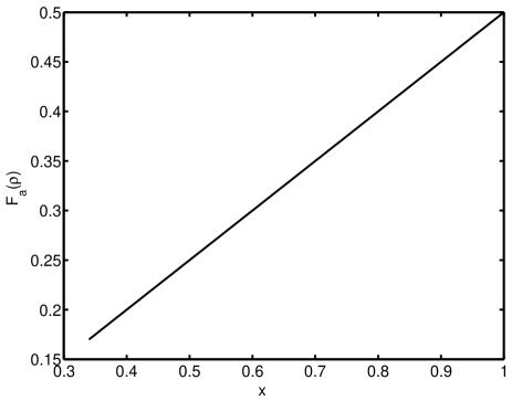
Figure 2: $F_{a}(\rho)$ of the mixed state $\rho(x)=x\left|GHZ\right\rangle\left\langle GHZ\right|+(1-x)/2(\left|W\right\rangle\left\langle W\right|+\left|\tilde{W}\right\rangle\left\langle\tilde{W}\right|)$  vs $x$, $x\in(1/3,1].$

IV Conclusion and Discussion

In summary, we have introduced an intuitive mathematical formulation to generalize the original tripartite entanglement to higher dimensional tripartite systems according to the tensor treatment of a tripartite pure state. A distinct characteristic of the present generalization is that the formulation for higher dimensional systems is invariant under permutation of the qudits. When the formulation is reduced to tripartite systems of qubits, there exists an exponent $\frac{1}{2}$ different from the original one, but the change of exponent provides convenience for the generalization to mixed states. The formulation for pure states can be conveniently extended to the case of mixed states by utilizing the kronecker product approximate technique. We have presented three different lower bounds for $F(\rho)$ of mixed states. The forms of the three results for mixed states are similar to those of bipartite entanglement [7,8]. All of them can provide necessary conditions to test the existence of tripartite entanglement, but the sufficiency of them may be different. However, because the dimension of $A_{\alpha\beta\gamma}$ is much higher than that corresponding to bipartite entanglement, it seems to be a bit difficult to directly apply to test the existence of tripartite entanglement of a general quantum mixed state. Fortunately, for the weakly mixed states, i.e. quasi pure states, one can find that our criterion can be conveniently applied and is even a sufficient condition for the existence of tripartite entanglement. In particular, our criterion can provide an analytic approximation. Since the 3-tangle is an entanglement measure, $F_{a}(\rho)$ is not only an existence criterion, but also an effective tripartite entanglement indicator. Even though there exist some questions left open, the intuitive mathematical formulation of tripartite entanglement and the convenient extension to mixed states will play an important role in the further understanding of multipartite entanglement measure.

V Acknowledgement

This work was supported by the National Natural Science Foundation of China, under Grant No. 60472017.

References

• (1) M. A. Nielsen and I. L. Chuang, Quantum Computation and Quantum Information (Cambridge University Press, Cambridge, 2000).
• (2) M. Zukowski, A. Zeilinger, M. A. Horne, and A. K. Ekert, Phys. Rev. Lett. 71, 4287 (1993).
• (3) C. H. Bennett, et al., Phys. Rev. Lett.70,1895 (1993).
• (4) C. H. Bennett and S. Wiesner, Phys. Rev. Lett. 69, 2881 (1992).
• (5) W. K. Wootters, Phys. Rev. Lett. 80, 2245 (1998).
• (6) A.Uhlmann, Phys. Rev. A 62, 032307 (2000).
• (7) K. Audenaert, F.Verstraete and De Moor, Phys. Rev. A 64, 052304 (2001).
• (8) Florian Mintert, Marek KuΕ›, and Andreas Buchleitner, Phys. Rev. Lett. 92, 167902 (2004).
• (9) Valerie Coffman, Joydip Kundu, and William K. Wootters, Phys. Rev. A 61, 052306 (2000).
• (10) Alexander Wong and Nelson Christensen, Phys. Rev. A 63, 044301 (2001).
• (11) A. Miyake, Phys. Rev. A 67, 012108 (2003).
• (12) Andreas Osterloh, Jens Siewert, Phys. Rev. A 72, 012337 (2005).
• (13) Chang-shui Yu, He-shan Song, Phys. Rev. A 72, 022333 (2005).
• (14) N. P. Pitsianis, Ph.D. thesis, Cornell University, New York, 1997.
• (15) C. F. Van Loan and N. P. Pitsianis, in Linear Algebra for Large Scale and Real Time Applications, edited by M. S. Moonen and G. H. Golub (Kluwer, Dordrecht, 1993), pp. 293-314.
• (16) Heng Fan, e-print quant-ph/0210168.
• (17) A. Peres, Phys. Rev. Lett. 76, 1413 (1996).
• (18) R. A. Horn and C. R. Johnson, Matrix Analysis (Cambridge University Press, New York, 1985).
• (19) Florian Mintert, AndrΓ© R. R. Carvalho, Marek KuΕ›, and Andreas Buchleitner, Physics Report 415, 207 (2005).
• (20) Tzu-Chieh Wei and Paul M. goldbart, Phys. Rev. A 68, 042307 (2003).