Influences of a longitudinal and tilted vibration on stability and dewetting of a liquid film

Abstract

We consider the dynamics of a thin liquid film in the attractive substrate potential and under the action of a longitudinal or a tilted vibration. Using a multiscale technique we split the film motion into the oscillatory and the averaged parts. The frequency of the vibration is assumed high enough for the inertial effects to become essential for the oscillatory motion. Applying the lubrication approximation for the averaged motion we obtain the amplitude equation, which includes contributions from gravity, van der Waals attraction, surface tension, and the vibration. We show that the longitudinal vibration leads to destabilization of the initially planar film. Stable solutions corresponding to the deflected free surface are possible in this case. Linear analysis in the case of tilted vibration shows that either stabilization or destabilization are possible. Stabilization of the dewetting film by mechanical action (i.e., the vibration) was first reported by us in PRE 77, 036320 (2008). This effect may be important for applications.

I Introduction

Dynamics of thin liquid films was extensively studied during the last decade both experimentally and theoretically. The importance of such studies is emphasized by the needs of modern nano and microfluidic technologies, which commonly employ films in the $100-1000\AA$ thickness range. Reviews focusing on different subfields of research include Refs. SHJ ; Oron ; Eggers , as well as twelve reviews focusing on wetting in the recent volume [Annu. Rev. Mater. Res. 38, (2008)].

It is well-known that very thin liquid films tend to dewet from the substrate (rupture). The primary cause for dewetting is the attractive van der Waals interaction of the film and the substrate. Loss of stability and rupture of liquid sheets is often undesirable and may lead to a technological or manufacturing process failure. Thus understanding dewetting and finding means to control it are the important and challenging problems.

One of the frequently used methods for controlling the fluid flow on small-to-large spatial scales is the application of the high frequency vibration AverBook ; TVC ; LChbook . Several phenomena may emerge when such vibration is applied, such as the oscillatory (pulsatile) fluid motion (Faraday instability) and the time-averaged fluid motion. Analyses of the pulsatile motion of the liquid layer and thin drops are carried out in Refs. LChbook ; wolf-70 ; Mancebo for the transversal vibration and in Refs. LChbook ; Hocking_Davis ; Oron_Gottlieb for the longitudinal one.

The standard high-frequency approximation is based upon the assumption of the vibration frequency so large, that the viscosity is important only in a thin boundary layer near the rigid wall AverBook ; TVC . This approximation works well for macroscopic films LChbook ; Lapuerta ; Thiele , but it fails for the thin films. Nonetheless, we have recently demonstrated PRE_vert that a hierarchy of typical times allows for the averaged description in a thin film system. Instead of using the standard high-frequency approximation, we assume that the vibration period $2\pi/\omega$ is (i) of the order of the characteristic time of the transversal transfer of the momentum, $\hat{H}_{0}^{2}/\nu$, and (ii) is small compared to the typical “horizontal time”, $L^{2}/\nu$. (Here $\hat{H}_{0}$ is the mean film thickness, $\nu$ is the kinematic viscosity, and $L$ is the typical horizontal scale. $L\gg H$ for the thin film.)

Reference PRE_vert develops the averaged description for the case of the vertical vibration of the substrate. We show that the influence of the vibration is finite if the amplitude is large in comparison with $\hat{H}_{0}$. In this case the vibration is the efficient way to stabilize the film against the van der Waals rupture. In this paper the approach of Ref. PRE_vert is extended to a longitudinal and a tilted vibration.

The paper is organized as follows. In Sec. II the problem is formulated: the governing equations and the dimensionless parameters are introduced for the case of the longitudinal vibration. Also in this section, using the separation of the time scales, we split the nonlinear boundary value problem for the fluid flow into two coupled boundary value problems for the pulsatile and for the averaged flows. The pulsatile flow is analyzed in Sec. III. The averaged amplitude equation for the film height is obtained in Sec. IV using the solution of the pulsatile flow. The linear stability problem for the amplitude equation, the weakly nonlinear analysis and the numerical results on film dynamics are presented in Sec. V. Stability of the pulsatile flow is demonstrated in Section VI. This stability translates into a stability of the averaged flow and thus the averaged amplitude equation is validated. In Sec. VII the analysis of the previous sections is generalized to the case of a tilted vibration. The conclusions are presented in Sec. VIII.

II Formulation of the problem

We consider a three-dimensional (3D) thin liquid film of the unperturbed height $\hat{H}_{0}$ on a planar, horizontal substrate. The Cartesian reference frame is chosen such that the $x$ and $y$ axes are in the substrate plane and the $z$ axis is normal to the substrate (Fig. 1).

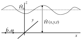
Figure 1: Problem geometry: the longitudinal vibration.

The substrate is subjected to the longitudinal harmonic vibration of the amplitude $\hat{b}$ and the frequency $\omega$. We assume that the system is not confined in the horizontal directions or the vertical boundaries are motionless. Thus the substrate motion induces the fluid motion due to viscosity and sloshing modes are not excited.

We assume the film height sufficiently small, so that the intermolecular interaction becomes important. In this paper, as in the preceding paper PRE_vert we consider the van der Waals attractive potential. Generalization to other models of wetting interactions is straightforward. Using same scalings as in Ref. PRE_vert [i.e., the units for the time, the length, the velocity and the pressure are $\hat{H}_{0}^{2}/\nu,\ \hat{H}_{0},\ \nu/\hat{H}_{0},\ \rho(\nu/\hat{H}_{0})^{2}$, respectively; $\nu$ is the kinematic viscosity and $\rho$ is the density of the liquid] we begin with the following dimensionless boundary-value problem:

$$\nabla\cdot{\bf v} = 0,$$ (1a)

$${\bf v}_{t}+{\bf v}\cdot\nabla{\bf v} = -{\bf\nabla}p+\nabla^{2}{\bf v}-G_{0}{\bf e_{z}},$$ (1b)

$${\bf v} = B\Omega\sin\Omega t{\bf e}_{x}\ {\rm at}\ z=0,$$ (2a)

$$h_{t}+{\bf v}\cdot{\bf\nabla}h = w,$$

$$\left(p+\phi-CaK\right){\bf n} = {\bf n}\cdot{\bf T}\ {\rm at}\ z=h(x,y,t).$$ (2b)

Here, ${\bf v}=({\bf u},w)$ is the fluid velocity (where ${\bf u}$ is velocity in the substrate plane and $w$ is the component normal to the substrate), $p$ is the pressure in the liquid, $\bf T$ is the viscous stress tensor, $h$ is the dimensionless height of the film, ${\bf e}_{x,z}$ are the unit vectors directed along the $x$ and $z$ axes, respectively, ${\bf n}=\left({\bf e}_{z}-\nabla h\right)/\sqrt{1+\left(\nabla h\right)^{2}}$ is the normal unit vector to the free surface, $K=\nabla\cdot{\bf n}$ is the mean curvature of the free surface, $\phi=-A/h^{3}$ [where $A=A^{\prime}/(6\pi\rho\nu^{2}\hat{H}_{0})$ is the non-dimensional Hamaker constant], $Ca=\sigma\hat{H}_{0}/(\rho\nu^{2})$ is the capillary number (where $\sigma$ is the surface tension), $G_{0}=g_{0}\hat{H}_{0}^{3}/\nu^{2}$ is the Galileo number, $B=\hat{b}/\hat{H}_{0}$ is the non-dimensional amplitude, and $\Omega=\omega\hat{H}_{0}^{2}/\nu$ is the non-dimensional frequency.

We consider the nonlinear evolution of the large-scale perturbations. Proceeding exactly as in Ref. PRE_vert , we first introduce a small parameter $\epsilon$, which is of the order of the ratio of the mean height $\hat{H}_{0}$ to the perturbation wavelength, i.e. $\epsilon\ll 1$ for long waves. Next, we introduce conventional stretched coordinates and the time

$$X=\epsilon x,\ Y=\epsilon y,\ T=\epsilon^{2}t,\$$

assume large capillary number $Ca=C\epsilon^{-2}$, and then separate the pulsations depending on the “fast” time $\tau\equiv\Omega t$ and the averaged variables which depend on the “slow” time $T$. The detailed analysis of this procedure is presented in PRE_vert ; it results in

$${\bf u} = \epsilon\bar{\bf U}+\tilde{\bf U},\ w=\epsilon^{2}\bar{W}+\epsilon\tilde{W},$$ (3a)

$$p = \bar{p}+\epsilon^{-1}\tilde{p},\ h=\bar{h}+\epsilon\tilde{h},$$ (3b)

where all fields are $O(1)$ quantities. The pulsations (averaged variables) are marked by tildes (overbars). Substitution of Eqs. (3) in Eqs. (1) and (2) gives two sets of equations and boundary conditions for the pulsational and the averaged parts of the velocity, pressure and height.
(i) For the pulsations:

$$\tilde{W}_{Z} = -{\bf\nabla}\cdot\tilde{\bf U},\ \Omega\tilde{\bf U}_{\tau}=-{\bf\nabla}\tilde{p}+\tilde{\bf U}_{ZZ},$$ (4a)

$$\tilde{p}_{Z} = 0,$$ (4b)

$$\tilde{\bf U} = B\Omega\sin\tau{\bf e}_{x},\ \tilde{W}=0\ {\rm at}\ Z=0,$$ (4c)

$$\Omega\tilde{h}_{\tau} = -\tilde{\bf U}\cdot{\bf\nabla}\bar{h}+\tilde{W},$$

$$\tilde{\bf U}_{Z} = 0,\ \tilde{p}=0\ {\rm at}\ Z=\bar{h},$$ (4d)

Hereafter ${\bf\nabla}\equiv(\partial_{X},\partial_{Y},0)$ is a two-dimensional projection of the gradient operator onto the $X-Y$ plane.

(ii) For the averaged parts:

$$\bar{W}_{Z} = -{\bf\nabla}\cdot\bar{\bf U},\ \bar{p}_{Z}=-G_{0},$$ (5a)

$$\bar{\bf U}_{ZZ} = {\bf\nabla}\bar{p}+\langle\tilde{\bf U}\cdot{\bf\nabla}\tilde{\bf U}+\tilde{W}\tilde{\bf U}_{Z}\rangle,$$ (5b)

$$\bar{\bf U} = \bar{W}=0\ {\rm at}\ Z=0,$$ (5c)

$$\bar{p} = -\langle\tilde{p}_{Z}\tilde{h}\rangle-\phi(\bar{h})-C\bar{\nabla}^{2}h,$$

$$\bar{h}_{T} = -\bar{\bf U}\cdot{\nabla}\bar{h}-\langle\tilde{\bf U}{\bf\nabla}\tilde{h}\rangle+\bar{W}+\langle\tilde{W}_{Z}\tilde{h}\rangle,$$

$$\bar{\bf U}_{Z} = -\langle\tilde{\bf U}_{ZZ}\tilde{h}\rangle\ {\rm at}\ Z=\bar{h}.$$ (5d)

In the set (5) the angular brackets denote averaging with respect to the fast time $\tau$. The boundary conditions at the free surface have been shifted at the mean position $\bar{h}$. Moreover, we neglect all terms of order $\epsilon$ as they are unimportant for the further analysis. Note that the boundary value problem governing the oscillatory motion, Eqs. (4) is linear despite the finite intensity of the oscillatory motion, see Eq. (3a). Also it can be seen that the set (4) is decoupled from the set (5) and thus the solution of the former set can be immediately found. It is worth noting that $B=O(1)$ (in contrast to Ref. PRE_vert , where the amplitude of the vibration has to be large in order to provide a finite intensity of the longitudinal motion.)

III Pulsatile motion

III.1 Analysis of the general case

Here we assume stability of the pulsatile motion (see Sec. VI for the proof) and determine the solution of Eqs. (4). We seek the solution in the form

$$\tilde{\bf U} = B\Omega{\bf e}_{x}{\rm Re}\left[I(X,Y,Z)\exp{\left(i\tau\right)}\right],$$ (6a)

$$\tilde{W} = B\Omega{\rm Re}\left[K(X,Y,Z)\exp{\left(i\tau\right)}\right],$$ (6b)

$$\tilde{p} = 0,\ \tilde{h}=B{\rm Re}\left[H(X,Y)\exp{\left(i\tau\right)}\right].$$ (6c)

Substitution of this ansatz in Eqs. (4) gives the set of equations and boundary conditions governing the amplitudes of the pulsations:

$$K_{Z} = -I_{X},\ I_{ZZ}+\alpha^{2}I=0,$$ (7a)

$$I = -i,\ K=0\ {\rm at}\ Z=0,$$ (7b)

$$iH = K-Ih_{X},\ I_{Z}=0\ {\rm at}\ Z=\bar{h},$$ (7c)

where $\alpha^{2}=-i\Omega$.

The solution of the boundary value problem (7) is:

$$I = -i\frac{\cos\alpha(\bar{h}-Z)}{\cos\alpha\bar{h}},$$ (8a)

$$K = i\bar{h}_{X}\frac{1-\cos\alpha Z}{\cos^{2}\alpha\bar{h}},\ H=\frac{\bar{h}_{X}}{\cos^{2}\alpha\bar{h}}.$$ (8b)

Note that the amplitudes $K,I$, and $H$, generally speaking, depend on $Y$ via $\bar{h}$, but only the $X$-component of ${\bf\nabla}\bar{h}$ is important for the pulsatile motion.

Figure 2: Dependence of the real (a) and imaginary (b) parts of $I$, Eq. (8a). Lines 1-4 correspond to $\tilde{\Omega}=\Omega\bar{h}^{2}=0.1,\,2,\,10,\,100$.

Figure 3: The value of $I_{m}\equiv|I\left(Z=\bar{h}\right)|$ vs. $\tilde{\Omega}$.

Figure 2 shows $I_{r}$ and $I_{i}$ for various values of $\Omega$. (Hence and henceforth we use subscripts “$r$” and “$i$” to denote the real and the imaginary parts, respectively.) Figure 3 presents $I_{m}=|I\left(Z=H\right)|$ at the mean position $\bar{h}$. Plotting these figures we use the local frequency $\tilde{\Omega}\equiv\Omega\bar{h}^{2}$, which is determined through the local thickness of the layer. It is obvious that $I_{m}$ rapidly decays with increase of the vibration frequency. Note that $I_{m}^{2}\bar{h}_{X}$ is the amplitude of the surface deviation, $|H|$ (where, of course, $\bar{h}_{X}$ is not apriori known).

III.2 Limiting cases of oscillatory motion

Case $\Omega\gg 1$. At large $\Omega$ the solution of the pulsatile motion, Eq. (8), is small beyond the Stokes boundary layer adjacent to the substrate. Indeed, taking an obvious relation $2\cos\alpha\approx\exp(i\alpha)=\exp\alpha^{*}$ into account (the asterisk denotes the complex conjugation; here we assume that $\alpha_{r}>0$), one immediately arrives at

$$I = -ie^{-\alpha^{*}Z},$$ (9)

$$K = -2ie^{\alpha^{*}\left(Z-2\bar{h}\right)}\bar{h}_{X},\ H=4e^{-2\alpha^{*}\bar{h}}\bar{h}_{X}.$$ (10)

As Eq. (10) does not satisfy the no-slip condition, near the substrate this asymptotic formula has to be rewritten. Expanding $1-\cos\alpha Z$ in a power series at small $\alpha Z$ in Eq. (8b), we obtain

$$K=2\Omega Z^{2}e^{-2\alpha^{*}\bar{h}}\bar{h}_{X}\ {\rm at}\ Z\to 0.$$ (11)

Of course, Eqs. (10) and (11) do not match, since they are the opposite cases ($\sqrt{\Omega}Z\gg 1$ and $\sqrt{\Omega}Z\ll 1$, respectively) of the high-frequency approximation, $\Omega\gg 1$, for Eq. (8b).

Since only the exponentially small terms are neglected in Eqs. (9),(10) these asymptotic expressions can be extended even to moderate $\Omega$ with high accuracy. For instance, the line 4 in Fig. 2 is indistinguishable from the curve corresponding to Eq. (9a) at $\Omega=100$ ($|\alpha|=10$).

Case $\Omega\ll 1$. In the limit of small frequency the solution of the pulsatile problem, Eqs. (8) reads:

$$I = -i-\frac{\Omega}{2}Z\left(2\bar{h}-Z\right)+$$ (12a)

$$\frac{i\Omega^{2}}{24}Z\left(Z^{3}-4\bar{h}Z^{2}+8\bar{h}^{3}\right),$$

$$K = \frac{\Omega}{2}\bar{h}_{X}Z^{2}\left[1+\frac{i\Omega}{12}\left(Z^{2}-12\bar{h}^{2}\right)\right],$$ (12b)

$$H = \bar{h}_{X}\left(1-i\Omega\bar{h}^{2}-\frac{2\Omega^{2}}{3}\bar{h}^{4}\right).$$ (12c)

Terms up to $\Omega^{2}$ are held in the expansion of the general case solution, Eqs. (8). This accuracy is needed to provide the averaged effects at low frequency. The expression for $I$, Eq. (12a), explains the coincidence of the line 1 in Fig. 2(b) with the line $I_{i}=-1$. Indeed, the difference between these line is proportional to $\Omega^{2}\sim 10^{-2}$, which cannot be seen on the scale of the figure. On the contrary, the real part [see Fig. 2(a)] is proportional to $\Omega$ and the corresponding variations are sufficient.

Case $\Omega$ arbitrary and $\bar{h}=const.$ In this limit it is clear from Eqs. (8b) that the oscillatory flow is one-dimensional (1D) and there are no oscillations of the surface height. Thus in this case the flow is the oscillatory Couette flow generated by the vibration of the substrate in a layer with the free surface. Moreover, this flow differs from the well-known oscillatory Poiseuille flow:

$$I=i\left[1-\frac{\cos\alpha(\bar{h}-Z)}{\cos\alpha\bar{h}}\right],\\$$ (13)

only in an additive constant.

It is also important to note that Eqs. (9) describe the conventional “Stokes layer”, i.e. the 1D flow forced by a high-frequency oscillation of the rigid plane in a semi-infinite space.

IV Averaged motion

IV.1 Analysis of the general case

Using Eqs. (6), the problem for averaged fields, Eqs. (5), can be rewritten as follows (hereafter the overbars are omitted):

$$p_{Z} = -G_{0},\ W_{Z}=-{\bf\nabla}\cdot{\bf U},$$ (14a)

$${\bf U}_{ZZ} = {\nabla}p+\frac{1}{2}B^{2}\Omega^{2}{\rm Re}\left(I^{*}I_{X}+K^{*}I_{Z}\right){\bf e}_{x},$$ (14b)

$${\bf U} = W=0\ {\rm at}\ Z=0,$$ (14c)

$$h_{T} = -{\bf U}\cdot{\bf\nabla}h+W-\frac{1}{2}B^{2}\Omega{\rm Re}\left(I^{*}H\right)_{X},$$

$$\ {\bf U}_{Z} = -\frac{1}{2}B^{2}\Omega{\rm Re}\left(I_{ZZ}^{*}H\right){\bf e}_{x},$$

$$p = -\phi-C\nabla^{2}h\ {\rm at}\ Z=h.$$ (14d)

The evolutionary equation for $h$ [the first equation in Eqs. (14d)] can be rewritten in the form

$$h_{T}=-\nabla\cdot\int_{0}^{h}{\bf U}{\rm d}Z-\frac{1}{2}B^{2}\Omega{\rm Re}\left(I^{*}H\right)_{X}\ {\rm at}\ Z=h.$$ (15)

Analytical integration of this set of equations is performed in Appendix A. It results in the following nonlinear equation for $h$:

$$h_{T} = {\nabla}\cdot\left(\frac{1}{3}h^{3}{\nabla}\Pi_{0}\right)-\frac{1}{2}B^{2}\Omega^{2}\left(Q_{1}h^{2}h_{X}\right)_{X},$$ (16a)

$$\Pi_{0} \equiv -\phi(h)-C\nabla^{2}h+G_{0}h.$$ (16b)

$$Q_{1} = \frac{3\left(2g_{1}-\gamma g_{2}\right)}{\gamma^{2}\left(\cosh\gamma+\cos\gamma\right)^{2}},$$ (16c)

$$g_{1} \equiv \sinh\gamma\sin\gamma,\ g_{2}\equiv\sinh\gamma\cos\gamma+\sin\gamma\cosh\gamma$$

where $\gamma=\sqrt{2\Omega}h$. This equation is the central equation of the paper. The first three terms at the right-hand side are the conventional terms resulting from van der Waals attraction, capillarity and gravity. The term proportional to $B^{2}\Omega^{2}$ is the new term resulting from the longitudinal vibration of the substrate.

The dependence of $Q_{1}$ is given in Fig. 4. Note that $Q_{1}>0$ except for the narrow interval $5.268<\gamma<8.507$. There is also an infinite set of such intervals (the second one is at $11.69<\gamma<14.85$), but the corresponding absolute values of $Q_{1}$ are very small.

Figure 4: Dependence of the coefficient $Q_{1}$ entering Eq. (16) on $\gamma$.

It is clear that the longitudinal vibration along the $X$ axis assigns the preferential direction ($X$) in $X-Y$ plane. Thus the $O(2)$ group of symmetry, which is characteristic for the amplitude equations governing the thin films dynamics, is broken for Eqs. (16). However, the derived amplitude equation is still invariant under the transformation $X\to-X$.

IV.2 Limiting cases $\Omega\gg 1$ and $\Omega\ll 1$

We first notice that the averaged effects vanish in the limiting case of high frequency, $\Omega\gg 1$. With exponentially small error, the oscillatory velocity given by Eqs. (9) and (10) is 1D and uniform along the $X$ axis. Indeed, the only reason for the variations of the flow velocity stems from the variation of the film height $h$, and thus this nonuniformity is exponentially small. As all known mechanisms are based on the existence of a gradient of the kinetic energy for the pulsations TVC , it is clear that the uniform oscillatory flux is unable to produce the averaged flow. Therefore, an averaged flow cannot be produced neither in the boundary layer nor in the core region. This conclusion agrees well with the asymptotics of $Q_{1}$ at large $\gamma$:

$$Q_{1}\approx-\frac{6}{\gamma}\left(\sin\gamma+\cos\gamma\right)e^{-\gamma}.$$

Thus the only relevant limiting case is the case of low-frequency, $\Omega\ll 1$. Integration of the boundary-value problem for Eq. (14b) results in the following solution (see Appendix A for details):

$${\bf U} = -\frac{1}{2}Z(2h-Z){\nabla}\Pi_{0}-\frac{B^{2}\Omega^{2}}{2}U^{(v)}h_{X}{\bf e}_{x},$$ (17a)

$$U^{(v)} = Z-\frac{\Omega^{2}Z}{120}\left(Z^{4}+5hZ^{3}-20h^{2}Z^{2}+80h^{4}\right).$$ (17b)

Then the following equation for the film height is obtained:

$$h_{T}={\nabla}\cdot\left(\frac{1}{3}h^{3}{\nabla}\Pi\right)-\frac{1}{15}B^{2}\Omega^{4}\left(h^{6}h_{X}\right)_{X},$$ (18)

which agrees with the expansion of $Q_{1}\approx\gamma^{4}/30$ in Eq. (16c) at small $\Omega$.

It is seen in Eq. (18) that at $\Omega\ll 1$ the vibration impact is determined by the squared amplitude of the pulsatile acceleration. This conclusion is expected in view of the similar result for the vertical vibration.

V Film dynamics

V.1 Linear stability analysis

It is convenient to rescale the amplitude equation (16a) using $X=\sqrt{C/3A}\tilde{X}$, $Y=\sqrt{C/3A}\tilde{Y}$, and $T=C/(3A^{2})\tilde{T}$. [Recall that $\phi=-Ah^{-3}$.] This leads to

$$h_{\tilde{T}}={\tilde{\nabla}}\cdot\left[h^{3}{\tilde{\nabla}}\left(\tilde{G}_{0}h+\frac{1}{3h^{3}}-{\tilde{\nabla}}^{2}h\right)\right]-\tilde{V}\left(Q_{1}h^{2}h_{\tilde{X}}\right)_{\tilde{X}},\\$$ (19)

where $\tilde{V}=B^{2}\Omega^{2}/2A$ and $\tilde{G}_{0}=G_{0}/3A$.

Seeking the solution of Eq. (19) in the form $h=1+\xi$, where $\xi$ is a small perturbation, one obtains:

$$\xi_{\tilde{T}}={\tilde{\nabla}}^{2}\left[\left(\tilde{G}_{0}-1\right)\xi-{\tilde{\nabla}}^{2}\xi\right]-\tilde{V}Q_{1}\left(\gamma_{0}\right)\xi_{\tilde{X}\tilde{X}}.$$ (20)

Here $\gamma_{0}\equiv\gamma/h=\sqrt{2\Omega}$.

For the normal perturbation $\xi$ proportional to $\exp\left(i\tilde{k}_{X}\tilde{X}+i\tilde{k}_{Y}\tilde{Y}-\tilde{\lambda}\tilde{T}\right)$ the decay rate $\tilde{\lambda}$ is:

$$\tilde{\lambda}=\left(\tilde{G}_{0}-1+\tilde{k}^{2}\right)\tilde{k}^{2}-\tilde{V}Q_{1}(\gamma_{0})\tilde{k}_{X}^{2},$$ (21)

where $\tilde{k}^{2}=\tilde{k}_{X}^{2}+\tilde{k}_{Y}^{2}$ is the squared wavenumber. In terms of the original unscaled variables $\left(k_{X},k_{Y}\right)$

$$\lambda=\frac{1}{3}\left[G_{0}-3A+Ck^{2}\right]k^{2}-\frac{1}{2}B^{2}\Omega^{2}Q_{1}(\gamma_{0})k_{X}^{2}.$$ (22)

Figure 5: Decay rates $\tilde{\lambda}$ for $\tilde{G}_{0}=3.33\times 10^{-4},\,\tilde{k}_{Y}=0,\,\tilde{k}_{X}=\tilde{k}$. (a) $\Omega=0.1$. (b) $\Omega=2$, (c) $\Omega=20$. (a) and (b): dashed, solid and dash-dotted lines correspond to $\tilde{V}=0,\,200,\,500$, respectively; (c): dashed, solid and dash-dotted lines correspond to $\tilde{V}=0,\,2,\,5$, respectively.

Since $Q_{1}$ is positive except for the narrow intervals of $\gamma$ (see Fig. 4), longitudinal vibration destabilizes the film beyond these intervals [see Fig. 5(a) and Fig. 5(b)]. Furthermore, one can readily see that the vibration does not impact the behavior of perturbations with $\tilde{k}_{X}=0$ (longitudinal rolls). Thus stabilization of the film by application of the longitudinal vibration is possible only in 2D systems, where there is no flow in the $Y$-direction, i.e. $\tilde{k}=\tilde{k}_{X},\ \tilde{k}_{Y}=0$. Below we consider only the behavior of 2D perturbations, which are critical for the reasonable interval of frequencies.

The typical pictures of the decay rate for this case are shown in Fig. 5. For stabilization [Fig. 5(c)] one needs an extremely large frequency of the vibration. (Recall that $\Omega=20$ corresponds to $n=300\,{\rm MHz}$ for the water layer of the height $1000\AA$.)

It is obvious that $\tilde{k}_{0}$:

$$\tilde{k}_{0}^{2}=1+\tilde{V}Q_{1}\left(\gamma_{0}\right)-\tilde{G}_{0}$$ (23)

solves an algebraic equation $\tilde{\lambda}=0$. For $\tilde{k}<\tilde{k}_{0}$ an instability takes place.

V.2 Weakly-nonlinear analysis of 2D systems

Since only the monotonic instability is present, as the analysis in Sec. V.1 confirms, we need to analyze branching of stationary solutions. Based upon the results of Sec. V.1, we consider only the 2D system, i.e. $h=h(\tilde{X})$ for the stationary solution. Analyzing the periodic solutions of a given wavenumber $\tilde{k}$, we keep in mind that the obtained results are appropriate for the confined systems of the length $\tilde{L}\equiv\pi/\tilde{k}$. Indeed, due to symmetry the boundary conditions $h_{\tilde{X}}=0$ are imposed at $\tilde{X}=0,\tilde{L}$ for the periodic solution of given wavenumber $\tilde{k}$. The same boundary conditions should be set at the impermeable boundaries $\tilde{X}=0,\,\tilde{L}$ for the confined system. In this case the spectrum of the wavenumbers for the perturbations is discrete and bounded from below: $\tilde{k}^{(n)}\geq\tilde{k}^{(0)}\equiv\tilde{k}$, where $\tilde{k}^{(n)}$ is the $n$th eigen wavenumber corresponding to $(n+1)/2$ wavelength confined into the horizontal length of the system. Thus for $\tilde{k}>\tilde{k}_{0}$ the longwave instability does not occur. Moreover, as it is shown below, even for $\tilde{k}<\tilde{k}_{0}$ the growth of perturbations does not necessarily lead to a rupture in a confined system.

In the stationary case Eq. (19) can be integrated once. Due to symmetry, the integration constant is set equal to zero. Thus we obtain

$$\tilde{k}^{2}h^{\prime\prime\prime}+\left(h^{-4}+\tilde{V}\frac{Q_{1}}{h}-\tilde{G}_{0}\right)h^{\prime}=0.$$ (24)

Here the primes denote the derivatives with respect to $\zeta\equiv\tilde{k}\tilde{X}$, i.e. the solution is assumed to be $2\pi$-periodic in $\zeta$.

To study the weakly nonlinear behavior of the perturbation, we expand the surface deflection $h$ and the wavenumber $\tilde{k}$ in powers of small $\delta$:

$$h=1+\delta\xi_{1}+\delta^{2}\xi_{2}+\ldots,\ \tilde{k}=\tilde{k}_{0}+\delta^{2}\tilde{k}_{2}.$$ (25)

Substituting these expansions in Eq. (24) we collect the terms of equal order in $\delta$. The first-order equation is

$$\hat{L}\xi_{1}\equiv\tilde{k}_{0}^{2}\xi_{1}^{\prime\prime\prime}+\left[1+\tilde{V}Q_{1}\left(\gamma_{0}\right)-\tilde{G}_{0}\right]\xi_{1}^{\prime}=0.$$ (26)

Its solution has the form:

$$\xi_{1}=a\cos\zeta,$$ (27)

whereas $\tilde{k}_{0}$ is given by Eq. (23).

The second order equation is

$$\hat{L}\xi_{2}=\left(4-\tilde{V}F_{1}\right)\xi_{1}\xi_{1}^{\prime},$$ (28)

where

$$F_{1}\equiv\gamma_{0}^{2}\frac{d}{d\gamma_{0}}\frac{Q_{1}\left(\gamma_{0}\right)}{\gamma_{0}}.$$

The solution of Eq. (28) is

$$\xi_{2}=-\frac{4-\tilde{V}F_{1}}{12\tilde{k}_{0}^{2}}a^{2}\cos 2\zeta.$$

The third-order equation is:

$$\hat{L}\xi_{3}=\left[\left(4-\tilde{V}F_{1}\right)\xi_{1}\xi_{2}-\frac{1}{3}\left(10+\tilde{V}F_{2}\right)\xi_{1}^{3}-2\tilde{k}_{0}\tilde{k}_{1}\xi_{1}^{\prime\prime}\right]^{\prime},$$ (29)

where

$$F_{2}\equiv\frac{\gamma_{0}^{3}}{2}\frac{d^{2}}{d\gamma_{0}^{2}}\frac{Q_{1}\left(\gamma_{0}\right)}{\gamma_{0}}.$$

The solvability condition of this equation couples the correction $\tilde{k}_{2}$ and the amplitude of the surface deviation as follows:

$$\tilde{k}_{2}=\left[10+\tilde{V}F_{2}+\frac{\left(4-\tilde{V}F_{1}\right)^{2}}{6\tilde{k}_{0}^{2}}\right]\frac{a^{2}}{8\tilde{k}_{0}}.$$ (30)

If the term in the bracket is positive, then $\tilde{k}_{2}>0$ and the subcritical bifurcation takes place. It is obvious that the branching solution is unstable in this case. Otherwise, the supercritical bifurcation occurs and the stable stationary solution corresponding to the deflected surface emerges.

Figure 6: The domain in the parameter space, where the supercritical branching of the surface deviation takes place. $\tilde{G}_{0}=0$, but the curve is almost unchanged even for $\tilde{G}_{0}=0.5$.

The curve separating these two regions in the plane $(\tilde{V},\Omega)$ is shown in Fig. 6. It can be readily seen that the supercritical excitation exists only at the large enough values of $\tilde{V}$, when the destabilization effects are well pronounced. Nevertheless, this phenomenon is quite interesting and unexpected and requires an additional analysis.

V.3 Stationary periodic solutions

To study stationary periodic solutions of a finite amplitude we integrate Eq. (24) with the boundary conditions:

$$h^{\prime}=0\ {\rm at}\ \zeta=0,2\pi,$$ (31)

and the mass conservation condition:

$$\int_{0}^{2\pi}h{\rm d}\zeta=2\pi.$$ (32)

(Recall that for the equivalent confined system only half of the period should be taken, i.e. $\zeta<\pi$.) This boundary value problem was solved by the shooting method. The numerical results are presented in Figs. 7-10 for $\tilde{G}_{0}=3.33\times 10^{-4}$.

Figure 7: Variation of the maximal (the upper branches) and the minimal (the lower branches) thickness of the layer with $\tilde{k}$ for $\tilde{V}=10$ and $\Omega=1,\,1.5,\,2$ – solid, dashed, and dotted lines, respectively. For the former case ($\Omega=1$) the value of $\tilde{k}_{0}$ is marked. Stability of the corresponding solutions is indicated by arrows.

Figure 8: Variation of the maximal (the upper branches) and the minimal (the lower branches) thickness of the layer with $\tilde{k}$. (a) – $\tilde{V}=30,\ \Omega=1,\,1.5,\,2$ – solid, dashed, and dotted lines, respectively. (b) – sketch with marked $\tilde{k}_{0}$ and $\tilde{k}_{c}$: solid lines correspond to stable solutions, dashed lines – to unstable ones. Domains of attraction are shown by arrows.

The amplitude curves $h_{m}(k)$ are shown for $\tilde{V}=10$ and $\tilde{V}=30$ in Figs. 7 and 8, respectively. These figures confirm the results of the weakly-nonlinear analysis: the supercritical bifurcation takes place for $\tilde{V}=30$.

In Fig. 7 the value of $\tilde{k}_{0}$ is marked for $\Omega=1$ (solid line). For smaller $\tilde{k}$ instability of the flat surface gives rise to a rupture. The stationary solution exists only for $\tilde{k}>\tilde{k}_{0}$, i.e. all the curves in Fig. 7 represent unstable subcritical solutions. The lower branches of the amplitude curves in Fig. 7 can be thought of as the boundaries of the domains of attraction for the equilibrium state ($h=1$) in the framework of the evolutionary problem, Eq. (19) (or the similar equation with $\zeta=\tilde{k}X$ being introduced). An initial distortion of the surface $h_{0}(\zeta)$ with the trough deeper than $h_{m}$ necessarily leads to rupture, while an initial distortion with $h_{0}(\zeta)>h_{m}$ for any $\zeta,\,0<\zeta<2\pi$ decays with time resulting in the equilibrium state at $T\to\infty$ (see arrows in Fig. 7). Of course, this interpretation is not exact, as the whole variety of the initial states $h_{0}(\zeta)$ is characterized by the only value, $h_{m}$. Therefore, the domain of attraction has to be confined by a band of finite thickness. However, due to the fast growth of the attracting van der Waals potential with the decrease of $h$, $h_{m}$ is a perfect characteristic for the domain of attraction and the band thickness is rather small. Our numerical tests based on the finite-difference computation of Eq. (19) support this conclusion.

For larger values of $\tilde{V}$ the stable distorted surface is found within some interval, $\tilde{k}_{c}<\tilde{k}<\tilde{k}_{0}$, see the dashed and the dotted curves in Fig. 8(a) and a schematic plot in Fig. 8(b). In the latter figure domains of attraction and stability properties of the obtained solutions are also demonstrated. Again, the lower branch $h_{m}(\tilde{k})$ of the unstable solution can be thought of as the boundary of the domain of attraction: the rupture occurs for initial distortions with $\min h_{0}(\zeta)<h_{m}$; in the opposite case the initial perturbation decays and the stable branch is achieved (either the stable branch of solution for $\tilde{k}<\tilde{k}_{0}$ or $h=1$ for $\tilde{k}>\tilde{k}_{0}$). To the best of our knowledge, this problem provides the first example where a nonplanar free surface is stable in the presence of the attracting van der Waals potential.

Figure 9: The shape of the free surface for $\tilde{V}=30,\ \Omega=2$; $\tilde{k}=3,\,2.7,\,2.56$ – dotted, dashed, and solid lines, respectively. The solid line with smaller surface deformation corresponds to the stable state, another solid curve corresponds to unstable solutions as well as dotted and dashed ones.

The interval of existence of a stable solution is quite small and for $\tilde{k}=\tilde{k}_{c}$ a saddle-node bifurcation takes place, see Fig. 8(b). Both stable (with smaller values of $|h_{m}-1|$) and unstable (with larger values of $|h_{m}-1|$) branches of the solution disappear at $\tilde{k}=\tilde{k}_{c}$ and do not exist at smaller $\tilde{k}$.

The typical shapes of the surface along the dotted curve in Fig. 8(a) is presented in Fig. 9. For the smaller value of the wavenumber, $\tilde{k}=2.56$, bistability takes place, i.e. there are two stationary shapes, the stable and unstable one (with the smaller and larger surface deformation, respectively).

The bifurcation lines $\tilde{k}_{0}(\Omega)$ and $\tilde{k}_{c}(\Omega)$ are shown in Fig. 10. The stable states with the deformed free surface exist between the corresponding solid and dashed lines. The direct pitchfork bifurcation takes place within this interval of $\Omega$. Otherwise, the branching is subcritical.

Figure 10: Variation of $\tilde{k}_{*}$ with $\Omega$ for $\tilde{V}=20,\,30,\,40$ – lines 1–3, respectively. Here $\tilde{k}_{*}=\tilde{k}_{0}$ correspond to the pitchfork bifurcation (dashed lines) and $\tilde{k}_{*}=\tilde{k}_{c}$ (solid lines) correspond to the saddle-node bifurcations. Dash-dotted lines show the locus of cusp points, where $k_{0}=k_{c}$; these lines correspond to $k_{0}(V)$ along the line shown in Fig. 6.

It should be noted that $\tilde{k}_{c}>\tilde{k}_{0}^{(c)}$, where $\tilde{k}_{0}^{(c)}\equiv\tilde{k}_{0}$ for $\tilde{V}=0$, i.e. the critical wavenumber in absence of the vibration. This inequality ensures that rupture always occurs at $\tilde{k}<\tilde{k}_{0}^{(c)}$, i.e. there is no stable stationary states even with deformed free surface. Thus the longitudinal vibration cannot be applied for “nonlinear stabilization”, i.e. in order to produce stable distorted film with $\tilde{k}<\tilde{k}_{0}^{(c)}$.

VI Stability of the time-periodic motion (pulsatile flow)

VI.1 Reduction of the stability problem

The finite intensity of the time-periodic solution, Eqs. (3), (6), and (8), raises question of the solution stability. In order to show stability or instability, we return to the unscaled Eqs. (1) and (2) and represent the velocity, the pressure and the surface deflection in the form

$${\bf v}=\tilde{\bf U}+\epsilon\tilde{W}{\bf e_{z}}+{\bf V},\ p=\bar{p}+P,\ h=\bar{h}+\epsilon\tilde{h}+\Upsilon.$$ (33)

(Within this section we restore the bar for the averaged film height, $\bar{h}$.) Here in accordance with Eqs. (3) the dominant parts of the unperturbed velocity are the pulsatile one, while for the pressure field and the layer height the averaged parts dominate over the oscillatory ones. Next, we linearize Eqs. (1) and (2) with respect to the small perturbations ${\bf V},\,P$ and $\Upsilon$, assuming 2D perturbation ${\bf V}=(U,0,W)$. (We will show that such perturbations are critical in the sense that they occur prior to the onset of 3D instability.) Thus we arrive at the following boundary value problem:

$$U_{x} = -W_{z},$$ (34a)

$$U_{t} = -U_{0}U_{x}-UU_{0x}-WU_{0z}-P_{x}+\nabla^{2}U,$$ (34b)

$$W_{t} = -U_{0}W_{x}-UW_{0x}-P_{z}+\nabla^{2}W,$$ (34c)

$$U = W=0\ {\rm at}\ z=0,$$ (34d)

$$P = -\left(\bar{p}_{z}+\frac{3A}{\bar{h}^{4}}\right)\Upsilon-CaK^{(l)}+{\bf T}_{nn}^{(l)},$$

$${\bf T}_{nt}^{(l)} = 0,\ \Upsilon_{t}+U_{0}\Upsilon_{x}+U\bar{h}_{x}=W\ {\rm at}\ z=\bar{h}.$$ (34e)

Here we set

$$U_{0}=B\Omega{\rm Re}\left[I(z)\exp\left(i\Omega t\right)\right].$$ (35)

according to Eq. (6). Besides, we have neglected all terms of order $\epsilon$, for example $\tilde{W}$ and $\tilde{h}$. Thus with accuracy $O(\epsilon)$ the base flow can be thought of as 1D flow.

Components of the viscous stress tensor are linearized as follows near the unperturbed surface, $z=\bar{h}(X,T)$:

$$T_{nn}^{(l)} \equiv {\bf n}_{0}\cdot\left({\bf T}_{1}+\partial_{z}{\bf T}_{0}\Upsilon\right)\cdot{\bf n}_{0}+2{\bf n}_{0}\cdot{\bf T}_{0}\cdot{\bf n}_{1}$$ (36)

$$T_{nt}^{(l)} \equiv {\bf n}_{0}\cdot\left({\bf T}_{1}+\partial_{z}{\bf T}_{0}\Upsilon\right)\cdot{\bf t}_{0}$$ (37)

$$+{\bf n}_{1}\cdot{\bf T}_{0}\cdot{\bf t}_{0}+{\bf n}_{0}\cdot{\bf T}_{0}\cdot{\bf t}_{1},$$

where ${\bf T}_{1}$ is calculated over $U$ and $W$, ${\bf T}_{0}$ is the viscous stress tensor of the base flow [i.e. $T_{0xx}=2U_{0x},\ T_{0xz}=U_{0z},\,T_{0zz}=O(\epsilon)$], ${\bf n}_{0}$ and ${\bf n}_{1}$ (${\bf t}_{0}$ and ${\bf t}_{1}$) are the normal (tangential) vector for the unperturbed free surface $z=\bar{h}$ and the correction due to its perturbation $\Upsilon$, respectively:

$${\bf n}_{0} = \frac{{\bf e}_{z}-\bar{h}_{x}{\bf e}_{x}}{\sqrt{1+\bar{h}_{x}^{2}}},\ {\bf t}_{0}=\frac{{\bf e}_{x}+\bar{h}_{x}{\bf e}_{z}}{\sqrt{1+\bar{h}_{x}^{2}}},$$ (38)

$${\bf n}_{1} = -\frac{\Upsilon_{x}}{\sqrt{1+\bar{h}_{x}^{2}}}\left({\bf e}_{x}+\frac{\bar{h}_{x}}{1+\bar{h}_{x}^{2}}{\bf e}_{z}\right),$$ (39)

$${\bf t}_{1} = \frac{\Upsilon_{x}}{\sqrt{1+\bar{h}_{x}^{2}}}\left({\bf e}_{z}-\frac{\bar{h}_{x}}{1+\bar{h}_{x}^{2}}{\bf e}_{x}\right).$$ (40)

Finally, for the curvature we obtain:

$$K^{(l)}=-\frac{\Upsilon_{xx}}{\left(1+\bar{h}_{x}^{2}\right)^{3/2}}+3\frac{\bar{h}_{x}\bar{h}_{xx}\Upsilon_{x}}{\left(1+\bar{h}_{x}^{2}\right)^{5/2}}.$$ (41)

It is clear that the $x$-derivatives of the base state variables are $O(\epsilon)$ quantities and thus they can be omitted from the leading-order analysis. Indeed, the base state depends on $x$ only via the slow coordinate $X$, whereas the characteristic wavelength of perturbations is $O(1)$. For example, $U_{0x}=\epsilon U_{0X}$. Also, for the same reason the derivatives with respect to the slow time $T$ are omitted. This procedure is equivalent to the methods of frozen coefficients: neglecting $\epsilon$-terms above we assume that the base flow is 1D and locally $x$-independent. Moreover, the free surface is almost horizontal: according to Eqs. (38) one obtains ${\bf n}_{0}={\bf e}_{z}$ and ${\bf t}_{0}={\bf e}_{x}$, which significantly simplifies the formulas. As a result, the stability problem for the pulsatile motion reads:

$$U_{x} = -W_{z},$$ (42a)

$$U_{t} = -U_{0}U_{x}-WU_{0}^{\prime}-P_{x}+\nabla^{2}U,$$ (42b)

$$W_{t} = -U_{0}W_{x}-P_{z}+\nabla^{2}W,$$ (42c)

$$U = W=0\ {\rm at}\ z=0,$$ (42d)

$$\ P = \left(G_{0}+\frac{3A}{\bar{h}^{4}}\right)\Upsilon-\frac{C}{\epsilon^{2}}\Upsilon_{xx}+2\left(W_{z}-U_{0}^{\prime}\Upsilon_{x}\right),$$

$$U_{z} = -W_{x}-U_{0}^{\prime}\Upsilon,$$

$$\Upsilon_{t} = -U_{0}\Upsilon_{x}+W\ {\rm at}\ z=\bar{h}.$$ (42e)

The primes denote the $z$-derivatives of $U_{0}$. Equation (14a) is taken into account to calculate $\bar{p}_{z}$ entering Eq. (34e). Recall that $C=\epsilon^{2}Ca$.

Large factor $\epsilon^{-2}$ in normal stress balance [the first relation from Eqs. (42e)] results in $\Upsilon=0$, i.e. the surface is locally undeformable. This, in turn, means that the boundary value problem (42) is the stability problem for 1D flow, periodic in time. This problem, the so-called time-dependent Orr-Sommerfeld problem, is analyzed in Secs. VI.2 and VI.3.

VI.2 Orr-Sommerfeld problem for the pulsatile flow

It is well-known squire-33 that 2D perturbations are critical for either stationary or time-dependent Orr-Sommerfeld problem. This proves neglecting the $y$-component of $\bf V$ and allows to introduce in Eqs. (42) a streamfunction $\psi$. Setting

$$\Upsilon=0,\ U=-\psi_{z},\ W=\psi_{x}$$

and separating the $x$-coordinate by means of $\psi(x,z,t)=\hat{\psi}(z,t)\exp\left(ikx\right)$ we arrive at

$$D^{2}\hat{\psi}_{t} = -ik\left(U_{0}D^{2}\hat{\psi}-U_{0}^{\prime\prime}\hat{\psi}\right)+D^{4}\hat{\psi},$$ (43a)

$$\hat{\psi} = \hat{\psi}^{\prime}=0\ {\rm at}\ z=0,$$ (43b)

$$\hat{\psi} = D^{2}\hat{\psi}=0\ {\rm at}\ z=\bar{h},$$ (43c)

where $D^{2}\hat{\psi}\equiv\hat{\psi}^{\prime\prime}-k^{2}\hat{\psi}$. It is convenient to rescale the vertical coordinate and the time in such a way that $\bar{h}=1$. Keeping the same notations for the rescaled variables we obtain:

$$D^{2}\hat{\psi}_{t} = -ik\left(U_{0}D^{2}\hat{\psi}-U_{0}^{\prime\prime}\hat{\psi}\right)+D^{4}\hat{\psi},$$ (44a)

$$\hat{\psi} = \hat{\psi}^{\prime}=0\ {\rm at}\ z=0,$$ (44b)

$$\hat{\psi} = D^{2}\hat{\psi}=0\ {\rm at}\ z=1,$$ (44c)

where

$$U_{0}=R{\rm Re}\left[I_{0}(z)\exp\left(i\tilde{\Omega}t\right)\right],\ I_{0}=-i\frac{\cos\tilde{\alpha}(1-z)}{\cos\tilde{\alpha}}.$$

We again use the local oscillation frequency (cf. Sec. III)

$$\tilde{\Omega}=\Omega\bar{h}^{2},\ \tilde{\alpha}=\alpha\bar{h};$$

the Reynolds number $R$ is introduced as follows

$$R=B\Omega\bar{h}.$$ (45)

First, we show that any constant value $C_{0}$ can be added to the amplitude of the velocity oscillations $I_{0}(z)$. It can be readily seen that Eqs. (44) are invariant under transformation

$$\hat{\psi}\to\hat{\psi}\exp\left[\frac{ikR}{\tilde{\Omega}}{\rm Re}\left(iC_{0}e^{i\tilde{\Omega}t}\right)\right],\ I_{0}\to I_{0}+C_{0}.$$ (46)

Because $\hat{\psi}$ is transformed by the periodical in time factor, stability properties do not change under this transformation. In particular, setting $C_{0}=i$ we reduce $I_{0}$ to the velocity profile of the oscillatory Poiseuille flow, Eq. (13), or

$$I_{0}=i\left[1-\frac{\cos\tilde{\alpha}(1-z)}{\cos\tilde{\alpha}}\right]$$

in terms of rescaled coordinate.

Thus, the stability problem for the pulsatile flow is reduced to the Orr-Sommerfeld problem (44) for the oscillatory Poiseuille flow. In spite of the detailed studies of the modulated Poiseuille flow Singer ; Straatman ; Davis_annu ; Kerczek , there have been no papers that deal with the particular case of the zero mean value of the pressure gradient.

Intuitively, the flow in a finite layer is more stable than the flow in a semi-infinite space, i.e. the Stokes layer, which is known to be stable Davis_annu . Nevertheless, we give some results on the stability of the flow in Sec. VI.3, which confirm the above guess.

VI.3 Stability problem for the oscillatory Poiseuille flow

To solve the linear stability problem (44) for the time-dependent flow, we apply the following method. First, due to Floquet theorem the amplitude of streamfunction $\hat{\psi}$ can be represented in the form:

$$\hat{\psi}=e^{-\Lambda t}\hat{\Psi}(z,t).$$ (47)

Here $\hat{\Psi}(z,t)$ is the periodic function of time with the period $2\pi/\tilde{\Omega}$, which thus can be expanded in a Fourier series as follows:

$$\hat{\Psi}(z,t)=\sum_{-\infty}^{+\infty}\Psi_{n}(z)\exp\left(i\tilde{\Omega}nt\right).$$ (48)

Substituting this ansatz into Eqs. (44), we arrive at the chain of coupled boundary value problems for the Fourier component, $\Psi_{n}(z)$. Truncation of the series by replacing the upper and lower limits of summation with $N$($-N$), respectively, leads to the set of $4(2N+1)$ ordinary differential equations. This set has been solved by the shooting method. We followed several lower branches of the spectrum; well-pronounced stabilization of the flow with increase of $R$ was found for all the branches.

Figure 11: Floquet exponents $\Lambda$ vs. $k$ for $Re=50000$. Three lower branches of the spectrum (a)-(c) for $\tilde{\Omega}=0.2,\,1,\,5$ – dotted, solid, and dashed lines, respectively.

The example of the computations is presented in Fig. 11, where the three lower branches of the Floquet exponent $\Lambda$ are shown. The curves are obtained with $N=10$; the changes caused by larger $N$ cannot be seen on the scale of the figure. Therefore, the oscillatory Poiseuille flow is shown to be stable even for finite values of $\tilde{\Omega}$.

VII Vibration along the near-vertical axis

VII.1 General notes and the analysis of the pulsatile motion

In this section we briefly generalize the previous analysis (Secs. III-V and Ref. PRE_vert ) to the case of the vibration along the axis that is tilted at a certain angle $\beta$ to the substrate (see Fig. 12). It is obvious that at the finite values of $\beta$ the normal component of the acceleration is unimportant. Indeed, it is shown in Ref. PRE_vert that the impact of vertical vibration is finite only at large amplitudes: $B=O\left(\epsilon^{-1}\right)$, while the horizontal vibration becomes essential even at finite $B$. Therefore, the longitudinal component of the vibration velocity is determinative.

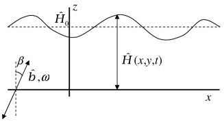
Figure 12: Problem geometry: the tilted vibration.

The only case where the effect of the normal acceleration can compete with the one due to longitudinal motion is the large-amplitude almost vertical vibration, i.e. $\beta\to 0$. This case is important for applications because in experiments it is difficult to ensure the absolutely vertical axis of the oscillatory motion – the horizontal components of accelerations occur inevitably.

Thus we assume $\beta$ small, i.e. $\cos\beta\approx 1$ and the near vertical motion of the substrate according to the law $z=z_{0}-B\cos\tau$ (in the laboratory reference frame). The fluid motion in the reference frame moving vertically with the substrate is governed by the Eqs. (1) and (2); the replacements are (i) the gravity modulation:

$$G(t)=G_{0}+B\Omega^{2}\cos\tau$$ (49)

and (ii) the longitudinal velocity is now $\beta B\Omega\sin\Omega t{\bf e}_{x}$ in Eq. (2a).

Assuming large vibration frequency $B$ we introduce the rescaled amplitude of the vibration $b\equiv\epsilon^{-1}B$ and the rescaled angle of the vibration $\mu\equiv\epsilon^{-1}\beta$. Thus the amplitude of the longitudinal motion of the substrate is $\mu b$ and the limiting case $\mu=0$ corresponds to the transversal vibration, i.e. the results of Ref. PRE_vert are reproduced. For the longitudinal vibration it is necessary to set $|\mu|\gg 1$, $b\ll 1$, while keeping the product, $B=\mu b$, finite in order to obtain the corresponding formulas from Secs. III-V.

Representing all fields as the sums of the pulsatile and averaged parts according to Eqs. (3) we arrive at the following equations for the pulsations:

$$\tilde{W}_{Z} = -{\bf\nabla}\cdot\tilde{\bf U},\ \Omega\tilde{\bf U}_{\tau}=-{\bf\nabla}\tilde{p}+\tilde{\bf U}_{ZZ},$$ (50a)

$$\tilde{p}_{Z} = -b\Omega^{2}\cos\tau,$$ (50b)

$$\tilde{\bf U} = b{\bf m}\Omega\sin\tau,\ \tilde{W}=0\ {\rm at}\ Z=0,$$ (50c)

$$\Omega\tilde{h}_{\tau} = -\tilde{\bf U}\cdot{\bf\nabla}\bar{h}+\tilde{W},$$

$$\tilde{\bf U}_{Z} = 0,\ \tilde{p}=0\ {\rm at}\ Z=\bar{h}.$$ (50d)

Here ${\bf m}\equiv\mu{\bf e}_{x}$. The averaged motion is described by Eqs. (5).

Representing the solution of the boundary value problem (50) in the form

$$\tilde{p} = b\Omega{\rm Re}\left[q(X,Y,Z)\exp{\left(i\tau\right)}\right],$$ (51a)

$$\tilde{\bf U} = b\Omega{\rm Re}\left[{\bf I}(X,Y,Z)\exp{\left(i\tau\right)}\right],$$ (51b)

$$\tilde{W} = b\Omega{\rm Re}\left[K(X,Y,Z)\exp{\left(i\tau\right)}\right],$$ (51c)

$$\tilde{h} = b{\rm Re}\left[H(X,Y)\exp{\left(i\tau\right)}\right].$$ (51d)

[cf. Eqs. (20) in PRE_vert and Eqs. (6)] and solving the equations for the amplitudes $q,{\bf I},K$, and $H$ we obtain (hereafter the bar over $\bar{h}$ is omitted again):

$$q = \Omega\left(h-Z\right),$$ (52a)

$${\bf I} = i{\bf\nabla}h-i{\bf M}\frac{\cos\alpha(h-Z)}{\cos\alpha h},$$ (52b)

$$K = -i\nabla^{2}h\left[Z+\frac{\sin\alpha\left(h-Z\right)-\sin\alpha h}{\alpha\cos\alpha h}\right]$$ (52c)

$$+i{\bf\nabla}h\cdot{\bf M}\frac{1-\cos\alpha Z}{\cos^{2}\alpha h},$$

$$H = -{\nabla}\cdot\left[f\left(\alpha h\right)h{\bf\nabla}h\right]+\frac{{\bf m}\cdot{\nabla}h}{\cos^{2}\alpha h},$$ (52d)

where ${\bf M}\equiv{\bf\nabla}h+{\bf m}$ and

$$f(y)=1-y^{-1}\tan y.$$ (53)

Due to the linearity of Eqs. (50) the oscillatory flow is a superposition of the motions generated by a vertical [see Eqs. (42) in PRE_vert ] and a horizontal [Eqs. (8)] vibration.

Referring to Sec. III.2 as well as to Sec. III of Ref. PRE_vert , we do not present the limiting cases of the solution (52). Milestones of the stability analysis for the pulsatile velocity are given in Appendix B.

Generally speaking the solution (52) remains valid even for the complex-valued $\mu$ and ${\bf m}$. This permits to consider the vertical and horizontal vibration to be out-of-phase, but leads to the cumbersome equation for the averaged fields. Thus, hereafter we assume real ${\bf m}$.

VII.2 Amplitude equation and limiting cases

Solving the averaged problem using the procedure similar to the one in Appendix A, we arrive at the amplitude equation for the averaged height:

$$h_{T} = {\nabla}\cdot\left(\frac{1}{3}h^{3}{\nabla}\Pi\right)-\frac{1}{2}b^{2}\Omega^{2}{\bf\nabla}\cdot{\bf Q},$$ (54a)

$$\Pi = \Pi_{0}+\frac{b^{2}\Omega^{2}}{2}{\rm Re}H,$$ (54b)

$${\bf Q} = h^{3}\left[Q_{21}\nabla^{2}h{\bf M}+\left(Q_{22}{\bf M}+\frac{1}{3}{\bf m}\right)\cdot{\bf\nabla\nabla}h\right]$$ (54c)

$$+h^{2}Q_{1}{\bf M}{\bf M}\cdot{\bf\nabla}h,$$

$${\rm Re}H = -f_{r}h\nabla^{2}h-({\bf\nabla}h)^{2}+Q_{3}{\bf M}\cdot{\bf\nabla}h.$$ (54d)

Here $\Pi_{0}$ and $Q_{1}$ are given by Eqs. (16b) and (16c), respectively,

$$Q_{21} = 6q_{1}-2q_{2},\ Q_{22}=5q_{1}-q_{2}-\frac{1}{3},$$ (55)

$$Q_{3} = 2\frac{\cosh\gamma\cos\gamma+1}{\left(\cosh\gamma+\cos\gamma\right)^{2}},$$ (56)

$$f_{r} = {\rm Re}f\left(\alpha h\right)=1-\frac{\sinh\gamma+\sin\gamma}{\gamma\left(\cosh\gamma+\cos\gamma\right)}.$$ (57)

$$q_{1} = \frac{\sinh\gamma-\sin\gamma}{\gamma^{3}\left(\cosh\gamma+\cos\gamma\right)},\ q_{2}=\frac{\cosh\gamma-\cos\gamma}{\gamma^{2}\left(\cosh\gamma+\cos\gamma\right)}.$$ (58)

The variation of the coefficients $Q_{21},\,Q_{22}$, and $Q_{3}$ with $\gamma$ is shown in Fig. 13, whereas $f_{r}$ can be found in Fig. 6(a) of Ref. PRE_vert .

For 2D case, when $h$ depends on $X$ and $T$ only, the amplitude equation reduces to

$$h_{T} = \left(\frac{1}{3}h^{3}\Pi_{X}\right)_{X}-\frac{1}{2}b^{2}\Omega^{2}Q_{X},$$ (59a)

$$Q = Q_{1}\left(\gamma\right)h^{2}\left(h_{X}+\mu\right)^{2}h_{X}$$ (59b)

$$+Q_{2}\left(\gamma\right)h^{3}h_{XX}\left(h_{X}+\mu\right)+\frac{1}{3}\mu h^{3}h_{XX}$$

Here $Q_{2}\equiv Q_{21}+Q_{22}$, cf. Eq. (31b) in Ref. PRE_vert .

Equations (54) coincide with Eq. (16) at $|\mu|\gg 1,\,\mu b=B$ (the longitudinal vibration). Equations (59) for $\mu=0$ (the vertical vibration) coincide with Eqs. (30) in Ref. PRE_vert , but the corresponding 3D analogue reads

$$h_{T} = {\nabla}\cdot\left(\frac{1}{3}h^{3}{\nabla}\Pi\right)-\frac{1}{2}b^{2}\Omega^{2}{\bf\nabla}\cdot{\bf Q},$$ (60a)

$${\bf Q} = Q_{1}h^{2}\left({\bf\nabla}h\right)^{2}{\bf\nabla}h$$ (60b)

$$+h^{3}\left[Q_{21}\nabla^{2}h{\bf\nabla}h+Q_{22}{\nabla}h\cdot{\nabla\nabla}h\right],$$

${\bf M}$ must be replaced with ${\bf\nabla h}$ in the definition of $\Pi$, Eq. (54d). It is clear that ${\bf Q}$ differs from the one defined by Eq. (43c) in Ref. PRE_vert . This contradiction is caused by the calculation mistake in Ref. PRE_vert .

Figure 13: Left axis – the dependence of the coefficients $Q_{22}$ (solid line) and $Q_{3}$ (dashed line) in Eq. (54), on $\gamma$. Right axis – $Q_{21}\left(\gamma\right)$.

It is clearly seen that the amplitude equation (54) contains several cross terms, which are linear with respect to $\mu$ and proportional to the first derivative of $h$ with respect to $X$. These terms remove the degeneracy with respect to the replacement $X\to-X$. Only the invariance under the simultaneous transformation $X\to-X$ and $\mu\to-\mu$ holds. Thus the presence of the vertical vibration makes different the motion along the positive and negative directions of the $X$ axis. Indeed, the $X$-component of the oscillatory velocity is in-phase with the vertical component, whereas the projection of the pulsatile velocity on the $-X$ axis is in counter-phase. This phase shift results in the difference after averaging.

The corresponding limits for the general case of the tilted vibration give the following amplitude equations:

(i) low frequency ($\Omega\ll 1$):

$$h_{T} = \frac{1}{3}{\nabla}\cdot\left(h^{3}{\nabla}\bar{\Pi}\right)+b^{2}\Omega^{4}{\bf\nabla}\cdot{\bf Q}_{l},$$ (61a)

$${\bf Q}_{l} = \frac{h^{7}}{315}\left(\nabla^{2}h{\bf M}+9{\bf M}\cdot{\nabla\nabla}h\right)$$ (61b)

$$-\frac{h^{6}}{15}{\bf MM}\cdot{\bf\nabla}h,$$

$$\bar{\Pi} = \Pi_{0}-\frac{b^{2}\Omega^{4}}{15}{\bf\nabla}\cdot\left(h^{5}{\bf M}\right).$$ (61c)

For the vertical vibration this leads to Eq. (61a) with

$${\bf Q}_{l} = \frac{h^{7}}{315}\left(\nabla^{2}h{\bf\nabla}h+9\nabla h\cdot{\bf\nabla\nabla}h\right)$$ (62a)

$$-\frac{h^{6}}{15}\left(\nabla h\right)^{2}{\bf\nabla}h,$$

$$\bar{\Pi} = \Pi_{0}-\frac{b^{2}\Omega^{4}}{15}{\bf\nabla}\cdot(h^{5}{\bf\nabla}h)$$ (62b)

instead of Eq. (44) in PRE_vert . For the horizontal vibration Eq. (18) is reproduced.

(ii) high frequency ($\Omega\gg 1$):

$$h_{T} = \frac{1}{3}{\nabla}\cdot\left\{h^{3}{\nabla}\left[\Pi+\frac{b^{2}\Omega^{2}}{4}\left({\bf\nabla}h\right)^{2}\right]\right\},$$ (63a)

$$\Pi = \Pi_{0}-\frac{b^{2}\Omega^{2}}{2}{\bf\nabla}\cdot\left(h{\bf\nabla}h\right).$$ (63b)

It is obvious that the longitudinal component of the vibration has no impact in this limiting case (see the explanation in Sec. IV.2). Therefore, the obtained expression coincides with the corresponding equations obtained in Ref. Lapuerta as well as Eqs. (46) and (47) in PRE_vert .

VII.3 Stability analysis of the flat surface

Representing $h$ in the form $1+\xi$ and linearizing Eqs. (54) with respect to a small perturbation $\xi$ results in

$$\xi_{T} = \frac{1}{3}\nabla^{2}\left[\left(G_{0}-3A\right)\xi-\left(C+\frac{b^{2}\Omega^{2}}{2}f_{r}\right)\nabla^{2}\xi\right]$$ (64)

$$-\frac{b^{2}\Omega^{2}}{2}\left(\frac{3Q_{2}+1-Q_{3}}{3}\mu\nabla^{2}\xi_{X}+\mu^{2}Q_{1}\xi_{XX}\right).$$

Here $\gamma$ must be replaced by $\gamma_{0}$ in $Q_{j},\ j=1,2,3$ and $f_{r}$, because all the coefficients are calculated for the unperturbed state, $h_{0}=1$. Substituting $\xi$ proportional to $\exp\left(ik_{X}X+ik_{Y}Y-\lambda T\right)$ and separating real and imaginary parts of the decay rate we arrive at

$$\lambda_{r} = \frac{1}{3}k^{2}\left[G_{0}-3A+k^{2}\left(C+\frac{b^{2}\Omega^{2}}{2}f_{r}\right)\right]$$ (65)

$$-\frac{b^{2}\Omega^{2}}{2}\mu^{2}Q_{1}k_{X}^{2},$$

$$\lambda_{i} = -\frac{b^{2}\Omega^{2}}{2}\mu k^{2}k_{X}\left[\frac{\sinh^{2}\gamma-\sin^{2}\gamma}{3\left(\cosh\gamma+\cos\gamma\right)}+Q_{2}\right].$$ (66)

It can be readily seen that the impact of tilted vibration on the real part of the decay rate, $\lambda_{r}$, is the superposition of impacts from the vertical and horizontal vibration [cf. Eq. (72) in PRE_vert for the former case and Eq. (22) for the latter one]. The additional terms, linear with respect to $\mu$, provide only the imaginary part of $\lambda$.

Thus the vertical component of the vibration is unimportant for the longwave perturbations (with $k\rightarrow 0$), and in this case the tilted vibration, similar to the horizontal one, decreases the stability threshold (unless $Q_{1}<0$, see the discussion of Eq. (22)).

Again, the 2D perturbations ($k_{Y}=0,\,k_{X}=k$) are critical for $Q_{1}>0$ and longitudinal rolls ($k_{X}=0$) are critical for narrow intervals of $\Omega$, where $Q_{1}<0$. However, the latter case seems unrealistic as very high frequencies are needed.

In confined systems with a discrete spectrum of $k$ the competition of the stabilizing effect of the vertical vibration and the destabilizing effect of the horizontal one takes place.

It should be noted also that the emergence of the imaginary part of $\lambda$ is the indicator of the averaged transport in the system. Indeed, the perturbations are stationary in a reference frame moving along the $X$ axis with a constant velocity $\lambda_{i}/k_{X}$. However, such a longitudinal drag is not limited by the transport of perturbations: any admixture can be spread over the system by means of the tilted vibration. Thus the tilted vibration seems to be the novel way to transport microparticles or molecules, which is important in many microfluidic applications.

VIII Summary

We consider a thin liquid film on a planar horizontal substrate subjected to a high frequency vibration. In the absence of a vibration, the van der Waals attraction to the substrate destabilizes the film and causes its dewetting. In contrast to conventional averaging method, we assume that the period of the vibration is comparable to the time of viscous relaxation of perturbations across the layer. This allows us to apply the averaging method to the ultra-thin films. Such analysis was first developed in Ref. PRE_vert , where the vertical vibration is considered and is shown to enhance film stability.

This work is a natural extension of Ref. PRE_vert . We consider, separately, the longitudinal and the tilted vibration. In the former case the finite amplitude of the vibration results in destabilization of the layer. There is also a sequence of narrow intervals of the vibration frequency, where stabilization occurs in the two-dimensional problem. However, the frequency must be very high (at least $300\,{\rm MHz}$ for a water layer of the thickness $1000\ \AA$).

Another effect of the longitudinal vibration is the emergence of the supercritical branching at the sufficiently high intensity of the vibration. In this case the deformed free surface becomes stable, i.e. the instability of the flat surface does not necessarily lead to a rupture.

For the tilted vibration the longitudinal (destabilizing) component of the pulsatile velocity is shown to be dominant. The only case, where the competition of the vertical and the horizontal vibration occurs, is the almost vertical vibration of large amplitude. For this case the averaging procedure is carried out and the corresponding amplitude equation is obtained. This analysis allows to correct the three-dimensional generalization of the amplitude equation for the vertical vibration PRE_vert .

Linear stability analysis in the framework of the amplitude equation indicates that both destabilization and stabilization of the flat surface are possible in the case of tilted vibration. Stabilization takes place only in the confined systems, when the spectrum of perturbations is discrete and bounded from below.

Besides, the small perturbations are oscillatory, i.e. the drag takes place for the tilted vibration. This property can be very important for many microfluidic applications since some admixtures can be transported in the same manner as the perturbations.

IX Acknowledgements

S.S. is partially supported by the Foundation “Perm Hydrodynamics”.

Appendix A Solution of the averaged problem. Longitudinal vibration

The solution of the averaged boundary value problem, Eqs. (14), is sought in the form:

$$p = -G_{0}Z+\Pi_{0},$$ (67)

$${\bf U} = {\bf U}_{c}+\frac{b^{2}\Omega^{2}}{2}U_{v}{\bf e}_{x},$$ (68)

where $\Pi_{0}$ is given by Eq. (16b),

$${\bf U}_{c}=\frac{1}{2}Z\left(Z-2h\right){\bf\nabla}\Pi$$

is the “conventional” part of the longitudinal velocity, and its “vibrational” part is determined by the boundary value problem

$$U_{v}^{\prime\prime} = {\rm Re}\left(II_{X}^{*}+KI_{Z}^{*}\right),$$ (69a)

$$U_{v} = 0\ {\rm at}\ Z=0,$$ (69b)

$$U_{v}^{\prime} = -\frac{1}{\Omega}{\rm Re}\left(HI_{ZZ}^{*}\right)\ {\rm at}\ Z=h.$$ (69c)

It can be readily shown that

$$U_{v}={\rm Re}\int_{0}^{Z}KI^{*}{\rm d}Z-\int_{0}^{Z}{\rm d}\xi\partial_{X}\int_{\xi}^{h}|I|^{2}{\rm d}\eta$$ (70)

is the solution of Eqs. (69).

Substituting Eq. (68) with both known parts, ${\bf U}_{c}$ and $U_{v}$, into Eq. (15) one can obtain Eq. (16) after straightforward (but cumbersome) integration.

Appendix B Stability of the pulsatile flow. Tilted vibration

Here we only briefly analyze the stability of the pulsatile flow (52) as this analysis is quite similar to one given in Sec. VII of Ref. PRE_vert and Sec. VI of the present paper.

In order to study the behavior of short-wavelength perturbations, we again return to the unscaled system of equations (1) and (2) with the above-mentioned changes: (i) and (ii), see Sec. VII.1. The perturbed fields are

$${\bf v}=\tilde{\bf U}+\epsilon\tilde{W}{\bf e_{z}}+{\bf V},\ p=\epsilon^{-1}\tilde{p}+\bar{p}+P,\ h=\bar{h}+\epsilon\tilde{h}+\Upsilon.$$ (71)

The only difference of Eqs.  (71) from Eqs. (33) is the presence of the oscillatory part of the pressure, according to Eq. (52a). In Eq. (71) the oscillatory parts are given by Eqs. (52). Below we again omit the bar over $\bar{h}$.

Repeating the same procedure of the method of frozen coefficients, we arrive at the following set of equations governing the small-amplitude perturbations:

$$W^{\prime} = -{\bf\nabla}\cdot{\bf U},$$ (72a)

$${\bf U}_{t} = -{\bf U}_{0}\cdot{\bf\nabla}{\bf U}-W{\bf U}_{0}^{\prime}-{\bf\nabla}P+\nabla^{2}{\bf U}+{\bf U}^{\prime\prime},$$ (72b)

$$W_{t} = -{\bf U}_{0}\cdot{\bf\nabla}W-P^{\prime}+\nabla^{2}W+W^{\prime\prime},$$ (72c)

$${\bf U} = W=0\ {\rm at}\ z=0,$$ (72d)

$$\Upsilon_{t} = -{\bf U}_{0}\cdot{\bf\nabla}\Upsilon+W,\ {\bf U}^{\prime}+\nabla W=-{\bf U}_{0}^{\prime\prime}\Upsilon,$$

$$P = \left(\frac{b\Omega^{2}}{\epsilon}\cos\Omega t+G+\frac{3A}{h^{4}}\right)\Upsilon-\frac{C}{\epsilon^{2}}\nabla^{2}\Upsilon$$ (72e)

$$+2\left(W_{z}-{\bf U}_{0}^{\prime}\cdot\nabla\Upsilon\right)\ {\rm at}\ z=h.$$

Here the primes denote the $z$-derivatives and the base oscillatory velocity is

$${\bf U}_{0}=b\Omega{\rm Re}\left[{\bf I}(z)\exp\left(i\Omega t\right)\right].$$ (73)

This boundary value problem is a straightforward 3D extension of Eqs. (42), with two exceptions. Firstly, there is an additional term at the right-hand side of Eq. (72e), which comes from $-\tilde{p}_{z}\Upsilon$. Secondly, the base oscillatory velocity is 2D.

As it is shown in Ref. PRE_vert [see Eqs. (52) there], the presence of the two asymptotically large terms in Eq. (72e) allows to split the stability problem into two different problems: (i) the Faraday instability and (ii) the instability of the oscillatory flow with the undeformable free surface.

(i) The solution is based on the results by Mancebo and Vega Mancebo . This analysis gives Eq. (53) of Ref. PRE_vert :

$$b_{c}=\frac{\sqrt{C}\Phi_{MV}\left(\Omega h^{2}\right)}{\Omega^{2}h^{5/2}},$$ (74)

where $\Phi_{MV}$ is the function given in Fig. 4 of Ref. Mancebo .

(ii) It is easy to see that the stability problem for 2D base flow (73) can be reduced to Eqs. (44). Indeed, after the separation of the longitudinal coordinates according to $f(x,y,z,t)=\hat{f}(z,t)\exp(i{\bf k}\cdot{\bf R})$ and the obvious transformation

$$\hat{f}\rightarrow\hat{f}\exp\left[-ib\cos\Omega t{\bf k}\cdot\nabla h\right],$$

the base velocity (73) becomes locally 1D:

$${\bf U}_{0}=-b\Omega{\bf M}{\rm Re}\left[i\frac{\cos\alpha(h-Z)}{\cos\alpha h}e^{i\Omega t}\right].$$ (75)

Here $f$ is each of the fields $\{P,W,{\bf U}=(U,V),\Upsilon\}$, and $\bf k$ and $\bf R$ are 2D vectors in plane $x-y$.

Thus, we again exclude the constant part of the velocity, i.e. the first term in $\bf I$ by the periodical in time transformation similar to Eq. (46) (see Sec. VI.3). Now one can redirect the local $x$ axis along the vector $\bf M$ and introduce the streamfunction in order to obtain exactly the same Orr-Sommerfeld problem as Eq. (43). It has been shown in Sec. VI.3 that the latter flow is stable.

References

• (1) R. Seemann, S. Herminghaus, and K. Jacobs, J. Phys.: Condensed Matter 13, 4925 (2001).
• (2) A. Oron, S. H. Davis, and S. G. Bankoff, Rev. Mod. Phys. 69, (1997) 931.
• (3) J. Eggers, Rev. Mod. Phys. 69, (1997) 865.
• (4) J. A. Sanders and F. Verhulst, Averaging methods in nonlinear dynamical systems (Springer-Verlag, New York, 1985).
• (5) G. Z. Gershuni and D. V. Lyubimov, Thermal Vibrational Convection (Wiley, New York, 1998).
• (6) D. V. Lyubimov, T. P. Lyubimova, and A. A. Cherepanov, Dynamics of interfaces in vibration fields (Fizmatlit, Moscow, 2004) (in Russian).
• (7) G. H. Wolf, Phys. Rev. Lett. 24, 444 (1970).
• (8) F. J. Mancebo and J. M. Vega, J. Fluid Mech. 467, 307 (2002).
• (9) L. M. Hocking, S. H. Davis, J. Fluid Mech. 467, 1 (2002).
• (10) A. Oron, O. Gottlieb, Phys. Fluids 14, 2622 (2002).
• (11) V. Lapuerta, F. J. Mancebo, and J. M. Vega, Phys. Rev. E 64, 016318.
• (12) U. Thiele, J. M. Vega, and E. Knobloch, J. Fluid Mech. 546, 61 (2006).
• (13) S. Shklyaev, M. Khenner, and A. A. Alabuzhev, Phys. Rev. E 77, 036320 (2008).
• (14) H. B. Squire, Proc. R. Soc. London, Ser. A 142, 621 (1933).
• (15) B. A. Singer, J. H. Ferziger, and H. L. Reed, J. Fluid Mech. 208, 45 (1989).
• (16) A. G. Straatman, R. E. Khayat, E. Haj-Qasem, and D. A. Steinman, Phys. Fluids 14, 1938 (2002).
• (17) S. H. Davis, Annu. Rev. Fluid Mech. 7, 57 (1976).
• (18) C. von Kerczek and S. H. Davis, J. Fluid Mech. 62, 753 (1974).