Evaporation and fluid dynamics of a sessile drop of capillary size

Abstract

Theoretical description and numerical simulation of an evaporating sessile drop are developed. We jointly take into account the hydrodynamics of an evaporating sessile drop, effects of the thermal conduction in the drop and the diffusion of vapor in air. A shape of the rotationally symmetric drop is determined within the quasistationary approximation. Nonstationary effects in the diffusion of the vapor are also taken into account. Simulation results agree well with the data of evaporation rate measurements for the toluene drop. Marangoni forces associated with the temperature dependence of the surface tension, generate fluid convection in the sessile drop. Our results demonstrate several dynamical stages of the convection characterized by different number of vortices in the drop. During the early stage the street of vortices arises near a surface of the drop and induces a non-monotonic spatial distribution of the temperature over the drop surface. The initial number of near-surface vortices in the drop is controlled by the Marangoni cell size which is similar to that given by Pearson for flat fluid layers. This number quickly decreases with time, resulting in three bulk vortices in the intermediate stage. The vortices finally transform into the single convection vortex in the drop, existing during about $1/2$ of the evaporation time.

I Introduction

Evaporation of a liquid drop in an ambient gas is a well-known yet not completely solved problem of the classical physics (see, for example, Langmuir1918 ; Fuchs ). Past decade was marked by significant advance in experiment and progress in understanding several key aspects of evaporation process, in particular, the vapor diffusion from the sessile drop surface and the hydrodynamic effects within the evaporating drops Deegan97 ; Deegan ; HuLarsonEvap ; Popov1 ; HuLarsonMarangoni ; Girard ; Ristenpart . It was found, in particular, that the evaporating flux density is inhomogeneous along the surface and diverges on approach to the pinned contact line Deegan97 ; Deegan . The resulting inhomogeneous mass flow modifies the temperature distribution over the drop surface and, hence, the Marangoni forces associated with the temperature dependent surface tension. The convection inside a droplet Zhang ; Davis1 ; Davis2 ; Davis3 ; Davis4 ; Lozinsky ; Niazmand ; Rednikov ; Savino ; HuLarsonMarangoni ; Girard ; Xu appears quite different from the classical Marangoni convection in the systems with a simple flat geometry Benard ; Pearson . Thermal conductivity of the substrate can also influence the formation of flows within a liquid drop since it is the magnitude of the conductivity which determines the sign of the tangential component of the temperature gradient at the surface close to the contact line and, therefore, the direction of the convection Ristenpart . The observation of the distinct stages of the evaporation process PicknettBexon ; Shanahan1 ; Shanahan2 has revealed that the longest and dominating regime of the evaporation process is the constant contact area mode, where the contact line is pinned. As further the contact line gets depinned, the different regime, the constant contact angle mode switches on. Finally, the drying mode follows, in which the height, the contact area and the contact angle rapidly decrease with time.

Understanding the details of the drop dynamics and evaporation is crucial to many applications involving this process, including preparing ultra-clean surfaces Leenaars90 ; Marra91 ; Huethorst91 ; Matar01 , protein crystallography Denkov ; Dimitrov , the studies of DNA stretching behavior and DNA mapping methods Jing ; HuLarsonDNA ; Hsieh , developing methods for jet ink printing Park ; Jong ; Lim , and in many other fields (see, for example, Frohn ). The process of evaporation of the drop with the colloidal suspension in it is of interest for methods of fabrication of various structures on the substrate. One of the examples is the effect of evaporative contact line deposition, the so-called coffee-ring effect Deegan97 ; Deegan ; Govor ; HuLarsonCoffee ; Popov1 ; Popov2 . Other important example is the self-assembly of long-range-ordered nanocrystal superlattice monolayer Lin1 ; Lin2 ; Bigioni3 .

While the fundamentals of quasistationary evaporation behavior are established, to some extent HuLarsonMarangoni ; Girard , the full dynamical description of the liquid drop evaporation is yet not available. In this work we undertake a step towards such a description offering a quantitative approach which enables us to account for all the relevant components of the evaporation process, namely, the fluid dynamics, the vapor diffusion, and the spatial temperature distribution in an evaporating sessile drop. The calculation are carried out according to the following scheme: (i) We derive the equation yielding the shape of the sessile drop and find how the evaporation rate is influenced by the deviations of the drop shape from the ideal spherical cap caused by the gravitational force. (ii) We solve the diffusion equation describing the vapor kinetics and calculate the local evaporation flux from the surface of the drop as well as the resulting evolution of the drop evaporation rate with time. At this stage we take into account the nonstationary effects in a vapor diffusion and find that the dynamical corrections to the evaporation rate do not vanish exponentially, but decay as $\propto 1/\sqrt{t}$. (iii) We solve the thermal conduction equation and find the spatial temperature distribution in the drop. (iv) We solve the Navier-Stokes equations and derive the velocity field corresponding to the convection within the drop. (v) Finally we arrive at a full description of the time evolution of the temperature and the fluid convection in the drop and identify characteristic stages of the thermocapillary convection. To this end we take into account inertial terms in the Navier-Stokes equations, including the time derivatives.

To ensure self consistency of the derivation of the physical characteristics of the system we include the temperature variation over the drop surface (since the surface tension depends on temperature) into the boundary conditions for the fluid dynamics in the drop. Furthermore, we take into account that the velocity field influences the thermal conduction, since the velocities enter the thermal conduction equation. And, finally, we take into account that the local evaporation flux is related to the heat transfer and, hence, to the temperature gradient on the drop surface.

While the developed approach is quite general and thus applies to a wide variety of the evaporating problems, we focus here on the experimental situation corresponding to evaporation of the toluene sessile drop of the capillary size. The typical values of the characteristic parameters at $T_{0}=295$K are taken from Lide and are presented in the lower part of Table 1. The initial values which we use in our calculations are given in the upper part of Table 1 and correspond to the evaporating toluene drop containing the colloidal solution of gold nanoparticles. These nanoparticles stick to the drop surface making islands there and form a monolayer nanocrystal on the substrate after toluene dries out Lin1 ; Lin2 ; Bigioni3 .

Table 1: The parameter values used in the paper for modeling the evaporation and hydrodynamics of the drop. The tabular data are taken at $T_{0}=295$K from Lide .

Drop	Contact line radius	$r_{0}=0.2$ cm
parameters	Initial height	$h=0.1314$ cm
	Initial mass	$m_{0}=8.7\cdot 10^{-3}$ g
Toluene	Density	$\rho=0.87$ g/cm3
characteristics	Molar mass	$\mu=92.14$ g/mole
	Thermal conductivity	$k=1.311\cdot 10^{-3}$ W/(cm$\cdot$ K)
	Thermal diffusivity	$\kappa=k/(\rho c_{p})=8.86\cdot 10^{-4}$ cm2/s
	Kinematic viscosity	$\nu=6.4\cdot 10^{-3}$ cm2/s
	Dynamic viscosity	$\eta=\nu\rho=5.6\cdot 10^{-3}$ g/(cm$\cdot$ s)
	Specific heat	$c_{V}=1.51$ J/(g$\cdot$K)
	Thermal-expansion coefficient	$\beta=1.138\cdot 10^{-3}$ K-1
	Surface tension	$\sigma=28.3049$ g/s2
	Temperature derivative of surface tension	$\sigma^{\prime}=-\partial\sigma/\partial T=0.1189$ g/(s${}^{2}\cdot$ K)
	Capillary constant	$a=0.258$ cm
	Latent heat of evaporation	$L=300$ J/g
Toluene	Diffusion constant	$D=0.1449$ cm2/s
vapor	Saturated toluene vapor density	$u_{s}=1.27\cdot 10^{-4}$ g/cm3
characteristics	Mean free path	$\lambda=2.7\cdot 10^{-5}$ cm
Air	Thermal conductivity	$k_{a}=0.258\cdot 10^{-3}$ W/(cm$\cdot$ K)
characteristics	Dynamical viscosity	$\eta_{a}=1.82\cdot 10^{-4}$ g/(cm$\cdot$ s)
	Density	$\rho_{a}=1.2\cdot 10^{-3}$ g/cm3
	Kinematic viscosity	$\nu_{a}=\eta_{a}/\rho_{a}=0.15$ cm2/s

We have identified three major distinct dynamic stages of the Marangoni convection during the evaporation of the toluene drop. During the initial stage, vortices appear near the surface of the drop, during the second stage they grow, coalesce and rapidly migrate into the drop bulk, and, finally, a single vortex survives governing all the fluid dynamics of the thermocapillary effect in the system. We derive the temperature profiles, evaporation rates, and the velocity distributions for each stage of the convection and uncover the important role of the convective heat transfer and the effect of inertial terms in the Navier-Stokes equations in the evaporation dynamics.

The paper is organized as follows. In Sec. II we present basic equations and main analytical results along with the quantitative description of main dynamical processes. In particular, Sec. II.1 deals with the shape of a sessile drop. Various aspects of the vapor diffusion and the drop evaporation rates are discussed in Sec. II.2–II.4. The characteristic Marangoni numbers for the drop are found in Sec. II.5. Sec. II.6 makes use of a self-consistent approach for calculating the velocity field and the spatial temperature. In Sec. III we present our main results and discussion, including the experimental and theoretical data for the evaporation rates and contact angles, the dynamics of vortex structure and the temperature profile. Sec. IV contains discussion. The details of the developed numerical approach are described in Appendix A.

II Basic equations and formulas

II.1 The sessile drop shape

During the evaporation process a drop loses its mass, hence with time its volume decreases and the shape changes. In this section we present the quasistationary method for calculating the shape of a sessile drop based on the hydrostatic Laplace equation. The approach holds as long as viscous forces, which generally enter the boundary condition for the pressure, are small. The ratio of viscous to capillary forces is characterized by the dimensionless number $C_{a}=\eta\overline{v}/\sigma$, where $\overline{v}$ is the characteristic value of the velocity. In our case $C_{a}\approx 2\cdot 10^{-4}\ll 1$.

The Laplace equation states that the pressure difference $\Delta p$, taken at the different sides of the surface of the liquid in an arbitrary point equals $\sigma k$, where $k=1/{R_{1}}+1/{R_{2}}$ is the mean curvature of the surface and $\sigma$ is the surface tension LL6 . Taking into account the gravity, one finds that at the surface of the drop

$$k+\frac{\rho gz}{\sigma}=k+\frac{2f}{a^{2}}=const,$$ (1)

where the shape of the drop surface is defined by the relation $z=f(x,y)$ and $a=\sqrt{{2\sigma}/{(\rho g)}}$ is the capillary constant. The curvature of the surface of the drop is, in its turn, also expressed in terms of the function $f(x,y)$. Indeed, $k=-\mbox{Tr}(G^{-1}Q)$, where $G$ and $Q$ are matrices of the first and the second quadratic forms of the surface Dubrovin . Plugging in the surface equation $z=f(x,y)$ we find

$$G=\left(\begin{array}[]{cc}1+f_{x}^{2}&f_{x}f_{y}\\ f_{x}f_{y}&1+f_{y}^{2}\\ \end{array}\right),\qquad\qquad Q=\frac{1}{\sqrt{1+f_{x}^{2}+f_{y}^{2}}}\left(\begin{array}[]{cc}f_{xx}&f_{xy}\\ f_{xy}&f_{yy}\\ \end{array}\right).$$ (2)

Therefore,

$$k=-\mbox{Tr}(G^{-1}Q)=\frac{2f_{x}f_{y}f_{xy}-f_{xx}(1+f_{y}^{2})-f_{yy}(1+f_{x}^{2})}{(1+f_{x}^{2}+f_{y}^{2})^{3/2}}.$$ (3)

We consider a sessile drop with the axial symmetry, where $z=f(r)$, $r=\sqrt{x^{2}+y^{2}}$. Then Eq. (3) assumes the form

$$k=\frac{f^{\prime\prime}}{(1+f^{\prime 2})^{3/2}}+\frac{f^{\prime}}{r(1+f^{\prime 2})^{1/2}},$$ (4)

where prime denotes the derivative with respect to $r$. It is convenient to parametrize and separate the variables as BA1883 ; RBN :

$$r=r(s),\qquad z=z(s),$$ (5)

where $s$ is the arc length on the drop surface taken from the apex. The curvature radii are $R_{1}$ and $R_{2}$, where $R_{1}$ is the curvature radius in the meridian $rz$-plane, and $R_{2}$ is the second curvature radius. Both curvature radii can be expressed in terms of the angle $\phi$ between the normal vector to the drop surface and the symmetry axis. Namely,

$$\frac{1}{R_{1}}=\frac{d\phi}{ds},\qquad R_{2}=\frac{r}{\sin\phi}.$$ (6)

Also, $\partial r/\partial s=\cos\phi$, $\partial z/\partial s=-\sin\phi$ and $r(0)=z(0)=\phi(0)=0$. Introducing the curvature radius $R_{0}$ at the apex, we can rewrite the Laplace equation as

$$\sigma\left(\frac{d\phi}{ds}+\frac{\sin\phi}{r}\right)=\frac{2\sigma}{R_{0}}-\rho gz$$ (7)

and therefore

$$\frac{d\phi}{ds}=\frac{2}{R_{0}}-\frac{\rho gz}{\sigma}-\frac{\sin\phi}{r}.$$ (8)

Hence, for the column vector $\mathbf{y}=(r(s),\phi(s),z(s))^{T}$, where $T$ is the transposition operation, we have the set of first-order differential equations with Cauchy boundary conditions:

$$\frac{d\mathbf{y}}{ds} = \mathbf{f}(s,\mathbf{y}),$$ (9)

$$\mathbf{f}(s,\mathbf{y}) = \left(\cos\phi,\frac{2}{R_{0}}-\frac{\rho gz}{\sigma}-\frac{\sin\phi}{r},-\sin\phi\right)^{T},$$ (10)

$$\mathbf{y}(0) = \left(0,0,0\right)^{T},\qquad\mathbf{f}(0,\mathbf{y})=\left(1,\frac{1}{R_{0}},0\right)^{T},$$ (11)

where the last relationship ensures that $\phi(s)/r(s)\to 1/R_{0}$ for $s\to 0$. The Cauchy problem (9)-(11) can be solved using the fourth order Runge-Kutta method or the Adams-Bashforth method BA1883 . Therefore, given the values of $R_{0}$ and $s_{max}$, one finds the drop shape in the form of $\mathbf{y}(s)=(r(s),\phi(s),z(s))^{T}$.

The quantities that are measured in the experiment are the mass of the drop

$$m=\pi\rho\int_{0}^{s_{max}}r^{2}(s)\sin\phi(s)ds\,\,\,,$$ (12)

and the radius $r_{0}$ of the substrate to which the drop is pinned. Given the values of $R_{0}$ and $r_{0}$, one can easily find $s_{max}$, and, therefore, $m$. Inverting the function $m(R_{0},r)$ numerically, one can obtain the value of $R_{0}$ and a drop shape for a given mass $m$ and contact line radius $r_{0}$. We note that Eqs. (9)-(11) are exact for a sessile drop with axial symmetry.

The evaporation rate for a given drop shape can be obtained as

$$\left|\frac{dm}{dt}\right|=\int_{0}^{s_{max}}2\pi r(s)J(r(s))ds,$$ (13)

where $J(r(s))$ is the mass evaporated per second from unit area of the surface, i.e. the local evaporation flux.

II.2 Evaporation of the drop

Consider a sessile droplet resting on a flat substrate. The vapor concentration above the droplet is time dependent and inhomogeneous during the evaporation process. Since the diffusion of the vapor from a near-surface layer is slower than the evaporation LL6 , the vapor concentration at the surface of the drop is assumed to equal the saturation value $u_{s}$. Far above the drop, the toluene vapor concentration is negligible. The dynamics of the vapor concentration in the surrounding atmosphere is described by the diffusion equation

$$\frac{\partial u}{\partial t}=D\Delta u.$$ (14)

We carry out our calculations (see Sec. III and Appendix A) taking into account both time dependence of vapor concentration and the deviations of the sessile drop shape from a spherical cap. It is instructive to begin discussing the problem with the more simple case allowing for an analytical description. To this end we notice that if evaporation can be viewed as an adiabatic process in a sense that the vapor concentration adjusts fast enough to the change of the drop size (and shape) i.e. on the time scales much less than the droplet evaporation time $t_{f}$, then the diffusion equation (14) can be replaced by the Laplace’s equation $\Delta u=0$, and the evaporation kinetics can be considered as a steady state process. Indeed the time $t_{p}$ required for the Brownian particle to pass the characteristic length $r_{0}$ is $t_{p}=r_{0}^{2}/D\ll t_{f}$ under the experimental conditions $t_{p}\approx 0.2$ s and $t_{f}\approx 500$ s. At the same time it interesting as well to consider particular dependencies of the local evaporation rates on time. Our simulation results based on Eq. (14) for the drop with the fixed surface can be fitted with the power-law time dependence

$$J(r,t)=J(r,\infty)\left(1+\frac{Ar_{0}}{2\sqrt{Dt}}\right),$$ (15)

which is almost exact with the accuracy within 1% for $t>0.5$ s and $|r_{0}-r|>0.01$ cm (see Fig. 1). Here $J(r,t)=|D{\mathbf{\nabla}}u|$ is the local evaporation flux on the drop surface, and constant $A=0.966$ is the only fitting parameter. For the case of the spherical cap the asymptotic value of the evaporation flux density $J(r,\infty)$ can be related to $J(\xi,\theta)$ from Eq. (20). Eq. (15) and Fig. 1 confirm the above estimation that the vapor concentration becomes stationary under the condition $t\gg r_{0}^{2}/D$. At the same time, for $t=t_{f}$ the second term in (15) still exceeds $1\%$ of the first term. The time dependence $J(r,t)-J(r,\infty)\propto 1/\sqrt{t}$ in Eq. (15) is known for an isotropic diffusion when the vapor concentration is kept saturated on the fixed surface of the sphere Fuchs . This is also valid for a diffusion from a flat plane LL6 . Our results demonstrate that such dependence also takes place for an inhomogeneous diffusion from a fixed surface of the sessile drop.

We further derived the numerical results which take into account the time dependent drop profile (see Fig. 5). In particular, they show that the corrections for the evaporation rate due to the nonstationary effects may be up to $5\%$ of the resulting value.

Figure 1: (Color online.) Local evaporation flux density $J(r,t)$ from a fixed surface as a function on $r$ for $t=1,2,3,5,10,50,100,500,1000,4000$ seconds of the evaporation process, from top to bottom, respectively (black curves). The time dependence of the vapor concentration is taken into account, whereas the surface of the drop with $m=8.7$ mg is fixed. The surface is taken as a spherical cap (left panel) and as a sessile drop surface (right panel). The bottom line on the left panel (blue curve) represents $J(r,\infty)$ taken from the exact solution (20). The bottom line on the right panel (green curve) represents $J(r,\infty)$ for a sessile drop.

Deegan et al.Deegan reported an analytical solution for a stationary spatial distribution of the vapor concentration for a drop with the shape of a spherical cap. The problem was shown to be mathematically equivalent to that solved by Lebedev Lebedev , who obtained the electrostatic potential of a charged conductor having the shape defined by two intersecting spheres. Modifying the equations derived in Deegan ; Lebedev , we arrive at the following formula for the vapor concentration $u(\alpha,\beta)$ above the surface (25) of a spherical drop:

$$u(\alpha,\beta)=u_{\infty}+(u_{s}-u_{\infty})\sqrt{2(\cosh\alpha-\cos\beta)}\int_{0}^{\infty}\frac{\cosh\theta\tau}{\cosh\pi\tau}\frac{\cosh\beta\tau}{\cosh(\pi-\theta)\tau}P_{-1/2+i\tau}(\cosh\alpha)d\tau.$$ (16)

Here $\theta$ is the drop contact angle, $-\pi+\theta\leq\beta\leq\pi-\theta$, $u_{\infty}=0$, $\alpha$ and $\beta$ are the toroidal coordinates:

$$r=\frac{r_{0}\sinh\alpha}{\cosh\alpha-\cos\beta},\qquad z=\frac{r_{0}\sin\beta}{\cosh\alpha-\cos\beta}.$$ (17)

At the drop surface $\beta=\pi-\theta$, therefore $\xi=r/r_{0}={\sqrt{x^{2}-1}}/{(x+\cos\theta)}$, where $x(\xi,\theta)=\cosh\alpha$, hence,

$$x(\xi,\theta)=\cosh\alpha=\frac{\xi^{2}\cos\theta+\sqrt{1-\xi^{2}\sin^{2}\theta}}{1-\xi^{2}}.$$ (18)

The evaporation flux at the surface is

$$J=|D{\mathbf{\nabla}}u|=\frac{D}{r_{0}}(\cosh\alpha-\cos\beta)\left.\frac{\partial u}{\partial\beta}\right|_{\beta=\pi-\theta},$$ (19)

and, therefore,

$$J(\xi,\theta)=\frac{Du_{s}}{r_{0}}\left(\frac{\sin\theta}{2}+\sqrt{2}(x(\xi,\theta)+\cos\theta)^{3/2}\int_{0}^{\infty}\frac{\cosh\theta\tau}{\cosh\pi\tau}\tau\tanh(\pi-\theta)\tau P_{-1/2+i\tau}(x(\xi,\theta))d\tau\right).$$ (20)

After substituting $\xi=r/r_{0}$ and (18) in Eq. (20), one obtains $J(r)$. Fig. 2 shows $\log J(r)$ for drops with different values of the contact angle $\theta$.

Figure 2: Log-log plot of $J(r)$ for drops with different contact angles. Lines marked with $a,b,c,d,e$ correspond to values $\pi/120$, $\pi/6$, $\pi/4$, $\pi/3$, $23\pi/60$ of the contact angle $\theta$, respectively.

The total drop mass is

$$m=\frac{\rho\pi r_{0}^{3}}{6}\tan\frac{\theta}{2}\left(3+\tan^{2}\frac{\theta}{2}\right),$$ (21)

and the total evaporation rate is

$$\left|\frac{dm}{dt}\right|=2\pi r_{0}^{2}\int_{0}^{1}\frac{\xi J(\xi,\theta)d\xi}{\sqrt{1-\xi^{2}\sin^{2}\theta}}.$$ (22)

While it were possible to simplify the expression for the drop evaporation rate adapting the sessile drop shape to that of the spherical cap of the same mass (see Sec. II.4), and then integrate Eqs.(20), (22), we will employ a more general method and develop a description of the evaporation rate which takes into account altogether spatial and time variations of the vapor diffusion and the sessile drop shape.

II.3 Estimation for the evaporation time

In this section we derive estimates for the evaporation time of the drop, which in spite of their relative simplicity, offer, nevertheless, a fairly good description of the experimental results. Let us consider a spherical evaporating drop of radius $r_{0}=0.2$ cm, so that the vapor density is saturated at the drop surface and vanishes far away from the drop. The diffusion of the toluene vapor controls the evaporation process. The outward flow of the vapor through the concentric sphere around the drop of the radius $R$ is $J=-D\cdot 4\pi R^{2}{du}/{dR}$ and does not depend on $R$. Here $u$ is the vapor density on the surface of the sphere of radius $R$, and $D$ is the diffusion constant for the toluene vapor. Therefore, $R^{2}du/dR=-A$, where $A=J/(4\pi D)$. Since the vapor concentration far away from the drop is negligible, we obtain $u=A/R$, $A=r_{0}u_{s}$ and $J=4\pi Dr_{0}u_{s}$. On the other hand, the flow of molecules from the fluid drop is $J=-\rho d(4\pi r_{0}^{3}/3)/dt$. Therefore, $r_{0}dr_{0}/dt=-Du_{s}/\rho$, and the evaporation time of the drop can be written as

$$t=\frac{\rho}{u_{s}}\frac{r_{0}^{2}}{2D}.$$ (23)

Eq. (23) is a well-known result of the classical Maxwell’s theory of the evaporation (see, for example, Fuchs ). The diffusion constant for toluene vapor can be estimated as

$$D=\frac{1}{3}\langle v\rangle\lambda.$$ (24)

Here $\langle v\rangle=\sqrt{{8RT}/{(\pi\mu)}}=26035$ cm/s is the average velocity for the thermal motion of the vapor molecules, $\lambda$ is the mean free path which may be estimated as follows. We replace the toluene molecules by the impermeable balls of the diameter $d\sim 1$ nm (we found the estimate for the diameter by adding together the lengths of the chemical bonds and taking into account the molecule geometry). Therefore, the mean free path is $\lambda={1}/{(\pi\sqrt{2}nd^{2})}={kT}/{(\pi\sqrt{2}P_{0}d^{2})}\approx 2.7\cdot 10^{-5}\mbox{\ cm.}$ Here $n$ is the density of the toluene molecules in the toluene vapor. If we substitute the obtained values into the Eq. (24), we get the estimate $D\sim 0.23$ cm²/s. This qualitative estimate is about in $1.5$ times larger than the result obtained from comparison of our numerical results and the experimental data in Sec III.

Substituting the value of $D$ to the Eq. (23), we get the evaporation time of the spherical drop: $t\approx 594\mbox{\ s}$.

II.4 Approximating a sessile drop surface with spherical caps

Spherical caps offer a very simple model allowing for carrying out analytical calculations to the end and are thus widely used for the modeling of the droplet. The equation for the surface is

$$z(r)=\sqrt{\frac{r_{0}^{2}}{\sin^{2}\theta}-r^{2}}-\frac{r_{0}}{\tan\theta}.$$ (25)

Figure 3 shows surface of the sessile drop and three approximating spherical caps with the parameters listed in Table 2. The radius of the substrate is $r_{0}=0.2$ cm for all the drops. The first spherical surface has the contact angle of the sessile drop. The second spherical surface has the mass of the sessile drop. The third spherical drop has the height of the sessile drop.

As seen from the Fig. 3 and Table 2, the characteristics $m$, $h$ and $\theta$ of all three approximating spherical caps are quite close to those of the sessile drop. This is not the case for local parameters such as the local curvature of the sessile drop. As follows from Eq. (1), for the local curvature to be approximately constant along the drop surface, the condition $B_{o}=\rho ghr_{0}/(2\sigma\sin\theta)\ll 1$ has to be satisfied. Here $B_{o}$ is dimensionless number which is analogous to the Bond number.

Figure 3: (Color online.) The sessile drop surface (red curve) and three spherical caps (curves 1,2,3; see Table 2).

Table 2: Characteristics of the sessile drop and three spherical caps.

Parameters	sessile drop	cap 1	cap 2	cap 3
$m$, mg	8.7	9.95625	8.7	8.22035
$\theta$, radian	1.3032326	1.3032326	1.20453564	1.16292249
$h$, cm	0.13145179	0.152552	0.137494	0.13145179
$\lambda(\theta)={(\pi-2\theta)}/{(2\pi-2\theta)}$	0.145545	0.145545	0.189081	0.206135
curvature at top, cm-1	8.0611	9.64418	9.33673	9.17966
curvature at the contact line, cm-1	12.0727	9.64418	9.33673	9.17966

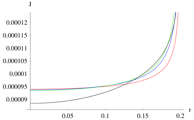
Figure 4: (Color online.) Black curve – $J(r)$ for the sessile drop with $m=8.7$ mg. Red, blue and green curves – $J(r)$ for the first, the second and the third spherical drop corresponding to notations of Table 2.

For our sessile drop $B_{o}\approx 0.4$; thus its curvature changes over the surface by factor of $1.5$. Furthermore, one sees from Fig. 4 and Table 2, that the assumption of the spherical cap shape cannot provide an approximation for the local evaporation flux density $J(r)$, which would have been accurate enough over a whole surface. At the same time, it is not surprising that the total evaporation rate, integrated over the surface of the drop, does not depend much on whether the drop is sessile or spherical. With the values from Table 1, one may numerically integrate (22) and obtain the evaporation rates for the three spherical drops: $dm_{1}/dt=20.52\ \ \mu\mbox{g/s}$, $dm_{2}/dt=19.76\ \ \mu\mbox{g/s}$, $dm_{3}/dt=19.47\ \ \mu\mbox{g/s}$. The difference is within a few per cent.

II.5 The Marangoni convection

A fluid convection within a drop caused by the temperature dependent surface tension which persists in the drop during the all stages of an evaporation process is called the Marangoni convection, and was first observed in its classical form by Bénard in a process of formation of the characteristic hexagonal convection patterns in flat fluid films. A theoretical description of the Marangoni convection was developed by Pearson Pearson . The Marangoni number $M_{a}$ (see Eq. (26) below) characterizes a relative importance of surface tension forces caused by the temperature variation and viscous forces, leading to the Benard-Marangoni instability if $M_{a}$ exceeds a critical value $M_{c}$. For a flat fluid film, $M_{c}\approx 83$ Pearson . To estimate the Marangoni number for a drop we exploit a formal similarity between a drop and a flat layer. We extract the temperature difference between the substrate plane and the apex of the drop from our simulation results as $\Delta T\approx 1$ K. The drop height $h$, the thermal conductivity $k$, the kinematic viscosity $\nu$, the specific heat $c_{V}$, and the rate of the change of the surface tension with the temperature, $-d\sigma/dT$, are taken from the Table 1. Then the value of the Marangoni number at the beginning of the drop evaporation process is

$$M_{a}=\frac{-\frac{d\sigma}{dT}(c_{V}\Delta T)h}{\nu k}\approx 2800.$$ (26)

According to experimental data, a turbulent regime arises for considerably larger values of the Marangoni number. For example, in the water drop the turbulence takes place for $M_{a}>22000$ Duan2005 . As the Reynolds number for toluene drop, $R_{e}\approx 62$, is also comparatively small, the flow in our problem is of a laminar character. A competition between the buoyancy-induced flow and the thermocapillary convection is characterized by the dimensionless number $B=\rho gh^{2}\beta/(7.14\sigma^{\prime})$ Pearson . In our case $B\approx 0.02\ll 1$, and the buoyancy-driven convection is negligibly small.

For a flat liquid layer the height of the Marangoni cell coincides with the layer thickness $h$, whereas the transverse size of the cell is determined by the characteristic instability wavelength $\lambda$. If the Marangoni number well exceeds the critical value, then $\lambda=2\pi h/\alpha$ and $\alpha=\sqrt{M_{a}/8}$ Pearson .

Our simulations show that near the surface a “street” of vortices forms at the initial stage of the convection (see Sec. III). The size of the vortices (i.e. the distance over which they extend into the bulk of the drop), $h_{d}$, constitutes a noticeable fraction of the height $h$ of the drop. With the assumption that the instability wavelength $\lambda$ and the Marangoni number can be described similarly to the case of flat liquid layer, one can take the value $h_{d}$ for the layer thickness and obtain $\lambda={2\pi\sqrt{hh_{d}}}/{\alpha}$. Taking as an example the number of the near-surface vortices $N=9$ and $s_{\text{m}ax}=0.256$ cm, we find $\lambda=s_{\text{m}ax}/N\approx 0.028$ cm and

$$h_{d}=\left(\frac{\lambda\alpha}{2\pi h}\right)^{2}h\approx 0.4\,h.$$ (27)

This although crude estimate turns out to be in a good agreement with our simulations for the Marangoni convection (see Figs. 6,7,8 and their discussions).

II.6 Hydrodynamic equations

The basic equations inside the drop are the Navier-Stokes equations, the continuity equation for the incompressible fluid, and the equation for thermal conduction

$$\frac{\partial\mathbf{v}}{\partial t}+(\mathbf{v}\nabla)\mathbf{v}+\frac{1}{\rho}\,{\mathrm{grad}\,p} = \nu\,\Delta{\mathbf{v}},$$ (28)

$$\mathrm{div}\,\mathbf{v} = 0,$$ (29)

$$\frac{\partial T}{\partial t}+\mathbf{v}\nabla T = \kappa\Delta T.$$ (30)

Here $\Delta=\partial^{2}/\partial r^{2}+\partial/r\partial r+\partial^{2}/\partial z^{2}$, $\nu=\eta/\rho$ is kinematic viscosity, $\kappa=k/(\rho c_{p})$ is thermal diffusivity. Other terms in the thermal conduction equation ${\nu}/{(2c_{p})}\left({\partial v_{i}}/{\partial x_{k}}+{\partial v_{k}}/{\partial x_{i}}\right)^{2}$, where sum over $i$ and $k$ is assumed, are negligibly small.

Applying the “$\mathrm{rot}\,$” operation to the both sides of equation (28), one excludes the pressure $p$ and obtains

$$\frac{\partial}{\partial t}\mathrm{rot}\,\mathbf{v}+(\mathbf{v}\nabla)\mathrm{rot}\,\mathbf{v}-(\mathrm{rot}\,\mathbf{v}\cdot\nabla)\mathbf{v}=\nu\Delta\mathrm{rot}\,\mathbf{v}.$$ (31)

Therefore,

$$\frac{\partial}{\partial t}\gamma(r,z)+(\mathbf{v}\nabla)\gamma(r,z)=\nu\left(\Delta\gamma(r,z)-\frac{\gamma(r,z)}{r^{2}}\right),$$ (32)

where the vorticity $\gamma$ is introduced by

$$\gamma(r,z)=\frac{\partial v_{r}}{\partial z}-\frac{\partial v_{z}}{\partial r};\qquad\mathrm{rot}\,\mathbf{v}=\gamma(r,z)\mathbf{i}_{\varphi}.$$ (33)

We define the stream function $\psi$, such that

$$\frac{\partial\psi}{\partial z}=rv_{r}\ ,\qquad\frac{\partial\psi}{\partial r}=-rv_{z}$$ (34)

One has $\partial^{2}\psi/(\partial r\partial z)=v_{r}+r(\partial v_{r}/\partial r)=-r(\partial v_{z}/\partial z)$, therefore $v_{r}/r+{\partial v_{r}}/{\partial r}+{\partial v_{z}}/{\partial z}=0$, i.e. the velocities obtained with Eqs.(34) will automatically satisfy the requirement (29).

Applying the Laplace operator to the stream function, one obtains $\Delta\psi=r\gamma-2v_{z}$, which can be transformed to a more convenient form $\tilde{\Delta}\psi=r\gamma$ with the modified operator $\tilde{\Delta}$ that differs from the Laplace operator by the sign of the term $\partial/(r\partial r)$:

$$\tilde{\Delta}\psi=\frac{\partial^{2}\psi}{\partial r^{2}}-\frac{1}{r}\frac{\partial\psi}{\partial r}+\frac{\partial^{2}\psi}{\partial z^{2}}=r\left(\frac{\partial v_{r}}{\partial z}-\frac{\partial v_{z}}{\partial r}\right)=r\gamma.$$ (35)

The method of the numerical solution is as follows: at each step, inside the drop

1. We solve Eq. (32) with the proper boundary conditions and find $\gamma(r,z)$;

2. We solve Eq. (35) and find $\psi(r,z)$. Then we find velocities with Eqs.(34);

3. We solve Eq. (30) and obtain the new boundary conditions for Eq. (32).

Details of the numerical approach are given in Appendix A. The proper boundary conditions for quantities $\gamma$ and $\psi$, satisfying Eqs. (32) and (35) respectively, are derived in Appendix B. They take the form $\gamma=0$ for $r=0$; $\gamma=\partial v_{r}/\partial z$ for $z=0$; $\gamma={d\sigma}/(\eta ds)+2v_{\tau}d\phi/ds$ on the surface of the drop; $\psi=0$ at all boundaries: at the surface of the drop, at the axis of symmetry of the drop ($r=0$), and at the bottom of the drop ($z=0$).

Here ${d\sigma}/{ds}=-\sigma^{\prime}\partial T/\partial s$ is the derivative of surface tension along the surface of the drop, where the distribution of temperatures, which is found with Eq. (30) is taken into account, and

$$\sigma(T)=\sigma_{0}-\sigma^{\prime}(T-T_{0}),$$ (36)

is the experimental dependence of surface tension $\sigma$ on temperature $T$.

The boundary conditions for the Eq. (30) are $\partial T/\partial r=0$ for $r=0$; $T=T_{0}$ for $z=0$;

$${\partial T}/{\partial n}=-{Q_{0}(r)}/{k}$$ (37)

on the surface of the drop. Here $Q_{0}(r)=LJ(r)$ is the rate of heat loss per unit area of the upper free surface, $J(r)$ is the local evaporation flux, $T_{0}$ is the temperature of the substrate, and $\mathbf{n}$ is a normal vector to the surface of the drop.

The relation $Q_{0}(r)=LJ(r)$ implies that the heat flow from ambient air towards the drop surface is negligible. This is the case if the temperature difference between the drop surface and the air far from the drop is less than $LDu_{s}/k$ Fuchs . This is well satisfied in the problem in question.

III Results

III.1 Evaporation rates

The evaporation rate of sessile drops is controlled mainly by the vapor diffusion in the surrounding atmosphere Deegan . Here we determined the diffusion coefficient of toluene vapor in air by measuring the toluene evaporation rate. The main conditions and parameters of the experiment are as follows. The sessile drop of $10\mu l$ of toluene is lying on a substrate and evaporates to the atmosphere during $\approx 500$ s. The contact line of the drop is pinned to the edge of the substrate. The weight of the drop was measured every $10$ seconds. As substrates, we used silicon wafers with a 100 nm thick amorphous silicon nitride layer.

The results of the measurements of drop evaporation rates are presented in Fig.5. Open circles are experimental values for the pure toluene evaporation and open triangles are values for the gold nanoparticles colloid. The solid line is the simulation result obtained in terms of Eq. (13) within the full numerical scheme. As seen in Fig. 5, it agrees well with the experimental data. Comparing the experimental data and the simulation results permits us to find the diffusion coefficient of the vapor, $D$, the only parameter controlling evaporation, as $D=0.1449$ cm²/s. It is worth noting that the rough estimate mentioned in Sec. II.3 is larger by the factor of about 1.5.

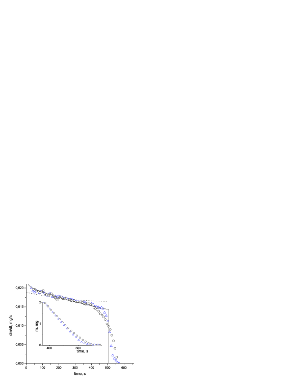
Figure 5: Drop evaporation rate $dm/dt$. Experimental data for the pure toluene evaporation (open circles) and Au nanoparticle colloid (open triangles). The solid line describes simulation results obtained within the full numerical scheme for the vapor diffusion (see also Sec. II.2). The dotted line is obtained assuming the local evaporation flux to be uniform over the drop surface and constant with time. Inset: Mass variation at the end of evaporation.

One can divide the evaporation process into three characteristic parts. Our simulation describes the main part, i.e. the quasi-stationary diffusion-limited evaporation, which lasts for about $400$ seconds. While there is a good agreement of the simulation and experimental data during the diffusion-limited regime of evaporation, this is not the case for the drying stage, i.e. the final 50-100 seconds. At the drying stage, the experimental evaporation rate drops rapidly but not abruptly. The main physical reason for such a behavior is the depinning of the contact line. The interface area then shrinks over time. The two distinct parts in the drying stage of evaporation can be identified. The first part, that occurs in the $t{=}400{-}510$ time window can be described as $dm/dt{\propto}(t_{0}{-}t)^{\alpha}$ that fits well the experimental data with $t_{0}{=}550(2)$, $\alpha{=}0.41(2)$ for the evaporation of the pure toluene and $t_{0}{=}522(3)$, $\alpha{=}0.28(8)$ for the colloid evaporation. The last part of the drying stage is a pronounced exponential decay of the evaporation rate $dm/dt{\propto}\exp(-t/t_{d})$, with the decay time $t_{d}{=}20.5(3)$ for the colloid evaporation. The exponential behavior during this stage qualitatively follows from the fact that change of the drop surface area $A$ controls here the evaporation rate evolution: ${dA}/{dt}\propto{dm}/{dt}\propto A$. Inset in Fig. 5 represents the experimental mass variation during the drying stage of the evaporation process.

III.2 Street of vortices and the dynamics of vortex structure

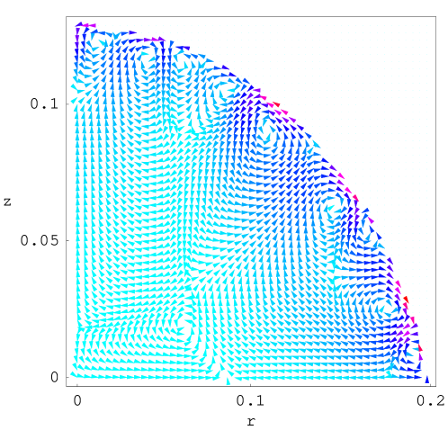
Figure 6: (Color online.) The velocity field at $t=0.16$ s.

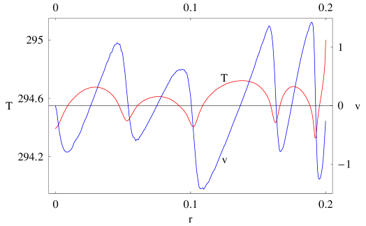
Figure 7: (Color online.) Temperatures (curve T) and velocities (curve v) along the drop surface as functions of the radius at $t=0.16$ s (compare with Fig. 6). The velocity changes its sign at crossing points with the horizontal axis.

Our calculations demonstrate the presence of the characteristic early regime in the dynamics of the Marangoni convection in an evaporating sessile drop. For various liquids and drop sizes, the vortices arise near the surface of the drop. For a toluene drop, this regime quickly arises and evolves up to $t\approx 0.3$ s. This is quite a short time period as compared with the total evaporation time $\approx 550$ s, but it admits an experimental study. The vortices grow, the number of vortices decreases, and eventually they evolve into the Marangoni convection cells in the bulk of the drop. This can be seen in Figs. 6,7, where the vortex structure contains six pairs of near-surface vortices and a corner vortex, and the temperature displays just six humps at the surface. As was shown in Sec. II.5, this number of vortices in the drop is controlled by the Marangoni cell size which is similar to that given by Pearson for flat fluid layers. The existence of near-surface vortices and the associated humps in the profile of the surface temperature, become more pronounced with the decrease of the viscosity of the liquid. There are no near-surface vortices when the viscosity increases more than in four times as compared with the toluene drop.

As seen in Fig. 7, the extrema of the surface temperature correspond to the change of sign of the tangential component of velocities at the surface. The reason for this behavior is that the fluid flow moves from the higher to the lower temperature regions of the surface, because, according to (36), the surface tension decreases with increasing the temperature. The flows result in a redistribution of the temperature due to the convective heat transfer. The number of the surface temperature humps and the number of the near-surface vortices decrease during their evolution.

The initial conditions chosen when generating Fig. 6 were: the vanishing velocities, constant room temperature, and the vanishing vapor concentration. For a description of a real experiment they have to be slightly modified to include the weak stochastic distribution of the surface temperature and velocities. We have carried out such calculations using a small-scale stochastic initial conditions. This has changed the particular behavior of the fluid dynamics only on the initial stage of the process, where a large number of small-scale surface vortices arise. Then the surface vortex structure quickly evolves into exactly the same one as we obtained for the basic initial conditions. This result demonstrates the generic character of the near-surface vortex regime in Fig. 6 at the early stage of the formation of the Marangoni convection.

An initial velocity field within the sessile drop can also be strongly disturbed right after the drop has fallen down on the substrate, or for some other reason. We model such a situation by choosing random initial conditions for the bulk velocity field, which are in agreement with the continuity equation (29). We find that strong disturbances of the bulk velocities can noticeably modify the initial stage of the drop dynamics, but they do not modify its main stage. For the initial random velocities of the order of $5$ cm/s (which well exceeds the typical velocity in the vortex $1$ cm/s), the difference between the dynamics of the disturbed and resting drops disappears after $t\approx 0.5$ s. This verifies the stability of the large-scale drop dynamics with respect to disturbances of the initial temperature and velocity fields.

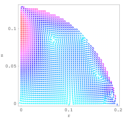
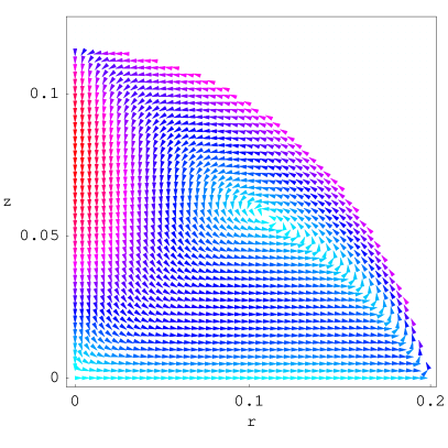
Figure 8: (Color online.) Left panel: The velocity distribution at $t=0.5$ s. The stage of drop dynamics with three vortices takes place from $t\approx 0.45$ s to $t\approx 2.0$ s. Right panel: The velocity distribution at $t=30$ s. A distribution with a single vortex takes place from $t\approx 2.0$ s to $t\approx 250$ s.

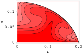
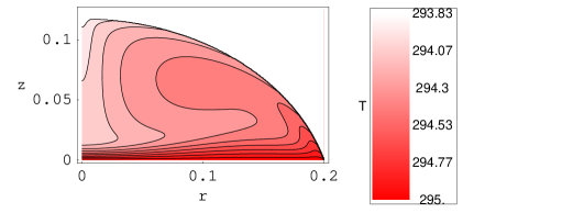
Figure 9: (Color online.) Distributions of temperature within drop for the stages of drop dynamics with three vortices (left) and a single vortex (right). The distributions are taken at $t=0.5$ s and at $t=30$ s. correspondingly. Temperature scale shown at the right column.

During the enlargement of the near-surface vortices, their number decreases, and the convection involves the bulk of the drop. As a result, for $t\approx 0.45$ s, three bulk vortices control the velocity and temperature fields in the drop, as seen in left panels in Figs. 8,9. During the coexistence of three vortices, the corner vortex starts growing at the expense of the other two vortices, and eventually at $t\approx 2.0$ s it occupies the whole drop volume. A spatial dependence of the temperature along the drop surface is nonmonotonic, if the drop contains more than one vortex (see Fig. 9). Right panels in Figs. 8,9 demonstrate how in the single-vortex regime effects of Marangoni forces drive liquid along the surface to the apex, where the fluid penetrates along the symmetry axis in the depth of the drop.

The regime with the single vortex represents one of the main stages of the dynamics of the evaporating sessile drop. It lasts up to $t\approx 250$ s. More than half of the drop mass evaporates during this period of time. If the initial values of mass, height and contact angle of the drop are $m=8.7$ mg, $h=0.1314$ cm, $\theta=1.2045$, then at the moment $t=250$ s we find $m=4.0$ mg, $h=0.0685$ cm, $\theta=0.716$. In particular, $h/(2r_{0})\approx 0.17$, i.e. the drop shape is noticeably flattened. The total time of the evaporation is $508$ s.

The quasistationary single-vortex state loses its stability at $t\approx 250$ s and the vortex acquires a pronounced nonstationary character. During this nonstationary regime, the fluid pulsations take place. The characteristic frequency of the pulsations corresponds to the circulation period $0.15$ s of a fluid element in the original vortex. Initially the pulsations are concentrated near the center of the original vortex. Then, as shown in Fig. 10, the single-cell pulsating state breaks into two-center (and later three-center) pulsating structure. Eventually at $t\approx 300$ s a quasistationary state with three vortices arises.

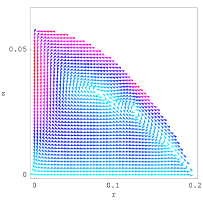
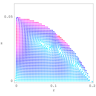
Figure 10: (Color online.) Fluid pulsations at $t=263$ s. (left panel) and at $t=281$ s. (right panel).

The numerical calculations of the fluid dynamics were tested with several different mesh sizes. The respective results are qualitatively identical and show reliable convergence of the quantitative characteristics. For example, the single-vortex regime was found to arise at $3.48$ s, $2.48$ s, $2.2$ s, $2.06$ s, $2.01$ s for 100$\times$100, 150$\times$150, 200$\times$200, 250$\times$250, 300$\times$300 mesh elements covering a half of the drop cross-section.

III.3 Temperature profile

If the thermal conductivity of a substrate is large compared to that of the liquid, then the temperature can be maintained practically constant at the substrate-fluid interface. This is the case, in particular, for the silicon nitride substrates used in experiments Lin1 ; Lin2 ; Bigioni3 . The silicon nitride is a material with high thermal conductivity, approximately in three orders larger than for the toluene. For this reason, the boundary condition for the temperature distribution at the substrate can be reduced to the constant temperature. Heat transfer between the substrate and the drop plays an important role in establishing the temperature profile in the drop. This also excludes a possibility for the reversal of the Marangoni convection Ristenpart , taking place for substrates with relatively small thermal conductivity.

Figure 11: Temperature profile along the surface as function of $r$, in disregarding the effect of fluid flow on the thermal conduction.

The characteristic scale of the temperature variation on the drop surface can be easily estimated if one disregards the effect of velocities on the thermal conduction. According to the evaporation rate data, the heat loss per unit area of the drop near apex is $Q_{0}=LJ(r=0)\approx 0.027$ W/cm² during the early stage of the evaporation process. Therefore, as follows from the boundary condition (37), we obtain $|\partial T/\partial n|=22.88$ K/cm. The calculations show that the temperature dependence is almost linear on $z$ at $r=0$ in disregarding the velocity term in thermal conduction. This permits to obtain the temperature difference between the substrate and the apex of the drop as $\delta T\approx\left|{\partial T}/{\partial n}\right|_{r=0}h_{0}=3.0087K$. This estimate is in a good agreement with the temperature profile along the surface shown in Fig. 11, where the effect of the velocity field on the temperature in Eq. (30) is disregarded. The temperature variation in Fig. 11 has larger amplitude and takes the monotonic form, as compared with the respective curve in Fig. 7. This demonstrates that the fluid flow noticeably modifies the temperature variations in the drop.

Similar consideration for the evaporating water drop studied in HuLarsonMarangoni results in $Q_{0}=0.093$ W/cm², $|\partial T/\partial n|=15.49$ K/cm, $\delta T\approx 0.56$ K. This estimation for the temperature difference exceeds in about $24$ times the respective numerical results obtained in HuLarsonMarangoni (see Figs. 1 and 2 there). We consider this discrepancy as an internal contradiction of HuLarsonMarangoni leading to a significant underestimation of the velocity values in the water drop. Our numerical calculations confirm that $\delta T\approx 0.6$ K for the water drop of HuLarsonMarangoni . At the same time, our calculations exactly reproduce the velocity field shown in Figs. 4 and 5 in HuLarsonMarangoni , if one takes a given surface temperature distribution of HuLarsonMarangoni . One should also note that the role of convective term in thermal conduction equation is substantially less for the water drop of HuLarsonMarangoni due to a small size of the drop.

III.4 Contact angles

The evaporation process with the pinned contact line is accompanied with an increase of the oblateness of the drop shape. Figure 12 displays our results for time dependence of the contact angle of sessile drop. Our results agree with the time-dependent contact angle determined experimentally under the identical initial drop parameters for the colloidal solution of gold nanoparticles in the toluene drop Lin2 . In Lin2 highly ordered nanoparticle islands were found to form on the drop surface. For this reason their orientation angle, which was determined experimentally close to the contact line with small angle X-ray scattering, coincides with the drop contact angle.

Figure 12: Contact angle of the drop during evaporation (solid line) and angle of NCS domains orientation extracted from experiment Lin2 (solid circles) as function of time.

IV Discussion

We have developed the approach for studying the evaporation and fluid dynamics of a sessile drop of a capillary size and applied it for the description of the toluene drop evaporation. In Lin1 ; Lin2 ; Bigioni3 the evaporating toluene drop containing colloidal solution of gold nanoparticles was used for realizing the self-assembly of nanocrystal monolayer. During the evaporation process, the nanoparticle islands were found to form on the drop surface Lin2 . For understanding the island formation as well as nanoparticle segregation, a study of the fluid and evaporation dynamics is necessary. In particular, the convective flows described in this paper are important for driving the nanoparticles to the contact line and the drop surface.

The numerical simulations were carried out and the system of the diffusion equation for the vapor, the thermal conduction equation for the temperature and the Navier-Stokes equations for the fluid flow in the drop is solved. The shape of the drop is controlled by the quasistationary Laplace equation, which includes the effect of the gravitational forces. Their role in forming a profile of a nonspherical sessile drop is characterized by dimensionless number $B_{o}=\rho ghr_{0}/(2\sigma\sin\theta)$, which is analogous to the Bond number. Since in our case $B_{o}\approx 0.4$, effect of gravitational forces, in general, should be taken into account. We have found that deviations of the sessile drop shape from the spherical cap are noticeable in local drop characteristics such as the local curvature and the evaporation flux density. At the same time the integrated over the drop surface characteristics, like the rate of the mass loss, are well described by the spherical cap approximation.

The experimental and simulation results for the time dependent drop evaporation rate agree well during the main longest stage of the evaporation process. The calculated evolution of the contact angle agrees with the results of Lin2 . In studying nonstationary diffusion equation, we found that the time-dependent corrections to the stationary local evaporation rates of the sessile drop do not vanish exponentially, but decay much slowly $\propto 1/\sqrt{t}$ with time and, in general, can be noticeable. This kind of behavior was established earlier only for homogeneous diffusion from a surface.

Our solution demonstrates the presence of several time stages in the evolution of the Marangoni convection in the drop. The main quasistationary fluid flow, containing only one vortex in the drop, is formed during the longest period of the evaporation process. Disregarding the time derivatives and the dynamical behavior of the quantities would result directly in a stationary state with one vortex in the sessile drop for a given contact angle. This kind of single-vortex solutions was obtained in previous theoretical studies of the sessile drop evaporation HuLarsonMarangoni ; Girard . Taking into account an explicit time dependence of all quantities, permitted us to identify a sequence of early dynamical stages of the Marangoni convection in the drop, containing a street of near-surface vortices which then transforms to the state with three bulk vortices. The stability of the large-scale drop dynamics with respect to perturbations of the initial conditions is identified. Also, for a flattened evaporating drop we found under the conditions in question a three-vortex state instead of the single-vortex one. We establish an important role of inertial terms in the Navier-Stokes equations and convective heat transfer terms in the thermal conduction equation.

Our further plans in developing the present approach include investigations of effects of surface surfactants and nanoparticles, effects of a nonstationary dynamics of the drop profile and a detailed study of the influence of substrate properties on the drop dynamics.

Authors thank H.M. Jaeger for fruitful and encouraging discussions. This research was supported by the U.S. Department of Energy Office of Science under the contract DE-AC02-06CH11357 and by the Program of Russian Academy of Sciences. L.Yu. Barash thanks the Dynasty Foundation for the partial support of his research.

Appendix A Numerical methods

A.1 A brief outline of the method

The simultaneous calculation of the physical quantities in the drop can be partitioned into several steps:

1. We apply to the diffusion equation (14) the implicit finite difference method using irregular mesh outside the drop and a variable time step. We use a boundary interpolation in a vicinity of the drop surface. For the boundary conditions we take $u=u_{s}$ on the drop surface, $u=0$ far away from the drop, $\partial u/\partial r=0$ and $\partial u/\partial z=0$ on the axes $r=0$ and $z=0$ correspondingly.

2. Calculations of the stream function $\psi$ and velocities $\mathbf{v}$ inside the drop are based on Eqs. (34), (35). The implicit finite difference method with a regular mesh inside the drop is applied. We use a boundary interpolation near the drop surface. For the boundary conditions we take $\psi=0$ at all boundaries: on the surface of the drop and on the axes $r=0$ and $z=0$.

3. We solve Eq. (32) to obtain the vorticity $\gamma$ inside the drop. The explicit finite difference method with a regular mesh inside the drop is used. We use a boundary interpolation close to the drop surface. For the boundary conditions we take $\gamma=0$ for $r=0$; $\gamma=\partial v_{r}/\partial z$ for $z=0$; $\gamma={d\sigma}/(\eta ds)+2v_{\tau}d\phi/ds$ on the drop surface, where ${d\sigma}/{ds}=-\sigma^{\prime}\partial T/\partial s$ is the derivative of the surface tension along the drop surface according to (36).

4. For calculating the temperature $T$ inside the drop, the explicit finite difference method with a regular mesh is applied to the thermal conduction equation (30). We use a boundary interpolation in a vicinity of the drop surface. The boundary conditions take the form $\partial T/\partial r=0$ for $r=0$; $T=T_{0}$ for $z=0$; ${\partial T}/{\partial n}=-{Q_{0}(r)}/{k}=-LJ(r)/k$ on the drop surface. Here $Q_{0}(r)$ is the rate of heat loss per unit area of the free surface, $\mathbf{n}$ is a normal vector to the drop surface.

5. During the iterative procedure, the drop shape is recalculated in accordance with the evaporative mass loss for the respective time interval. For this purpose we use the Runge-Kutta method for Eqs.(9)-(11).

A.2 Explicit method for temperatures inside the drop

For solving Eq. (30) the following explicit finite difference method is used:

$$\frac{T_{ij}^{n+1}-T_{ij}^{n}}{h_{t}}+v_{rij}\frac{T_{i+1,j}^{n}-T_{i-1,j}^{n}}{2h_{r}}+v_{zij}\frac{T_{i,j+1}^{n}-T_{i,j-1}^{n}}{2h_{z}}=\frac{\kappa}{h_{r}^{2}}(T_{i+1,j}^{n}-2T_{ij}^{n}+T_{i-1,j}^{n})+\\ +\frac{\kappa}{h_{z}^{2}}(T_{i,j+1}^{n}-2T_{ij}^{n}+T_{i,j-1}^{n})+\frac{\kappa}{2ih_{r}^{2}}(T_{i+1,j}^{n}-T_{i-1,j}^{n}),$$ (38)

which gives

$$T_{ij}^{n+1}=\alpha_{z}(T_{i,j+1}^{n}+T_{i,j-1}^{n})+\alpha_{r}(1+1/(2i))T_{i+1,j}^{n}+\alpha_{r}(1-1/(2i))T_{i-1,j}^{n}+(1-2\alpha_{r}-2\alpha_{z})T_{ij}^{n}-\\ -\beta_{r}v_{rij}(T_{i+1,j}^{n}-T_{i-1,j}^{n})-\beta_{z}v_{zij}(T_{i,j+1}^{n}-T_{i,j-1}^{n}).$$ (39)

Here $T_{ij}^{n}$ is the temperature at the $n$-th time step, $i,j$ are the coordinates on the regular mesh, $h_{r}$,$h_{z}$ are steps along the respective axis, $h_{t}$ is the time step,

$$\alpha_{r}=\kappa h_{t}/h_{r}^{2},\quad\alpha_{z}=\kappa h_{t}/h_{z}^{2},\quad\beta_{r}=h_{t}/(2h_{r}),\quad\beta_{z}=h_{t}/(2h_{z}).$$ (40)

For $r=0$ we have $\partial T/\partial r=0$, therefore for small $r$ one has $T=\alpha+O(r^{2})$, i.e. $\partial^{2}T/\partial r^{2}=\partial T/(r\partial r)$. Hence, instead of (39) we have the following formula:

$$T_{0j}^{n+1}=\alpha_{z}(T_{0,j+1}^{n}+T_{0,j-1}^{n})+4\alpha_{r}T_{1,j}^{n}+(1-2\alpha_{r}-4\alpha_{z})T_{0j}^{n}-\beta_{z}v_{z0j}(T_{0,j+1}^{n}-T_{0,j-1}^{n}).$$ (41)

For $z=0$ we have $T_{i0}=T_{0}$.

A.3 Boundary interpolation for temperatures inside the drop

Let $G=\partial T/\partial n=-LJ(r)/k$, and $D(i,j)$ is the mesh point which is close to the surface. The point $D$ is inside the drop and at least one of its nearest neighbors has to be outside the drop. In linear approximation $T=a+br+cz$ in a vicinity of the point $D(i,j)$. We denote the temperatures at points $B(i-1,j)$ and $C(i,j-1)$ as $u_{B}$ and $u_{C}$ correspondingly. Then

$$b\sin\phi+c\cos\phi=G,\qquad a+b(i-1)h_{r}+cjh_{z}=u_{B},\qquad a+bih_{r}+c(j-1)h_{z}=u_{C}.$$ (42)

The solution of the set of equations is

$$a = \left(h_{r}\cos\phi(iu_{B}-(i-1)u_{C})+h_{z}\sin\phi(u_{B}+j(u_{C}-u_{B}))-h_{r}h_{z}G(j+i-1)\right)/R$$ (43)

$$b = (h_{z}G+(u_{C}-u_{B})\cos\phi)/R$$ (44)

$$c = (h_{r}G+(u_{B}-u_{C})\sin\phi)/R$$ (45)

$$R = h_{r}\cos\phi+h_{z}\sin\phi.$$ (46)

The coefficients $a,b,c$ allow to calculate the temperature at the point $D(i,j)$ using the formula $T_{i,j}=a+bh_{r}i+ch_{z}j$. Also, the coefficients $a,b,c$ allow to find the temperature at the surface of the drop near the point $D$.

A.4 Alternating direction implicit method for vapor density

In order to cover quite a large region for the vapor density calculation with Eq. (14), this is convenient to use irregular mesh. We use the following mesh: $r_{i}=ih_{r}$ for $i<n_{r}$, $r_{i}=h_{r}(n_{r}+1.04^{i-n_{r}+79}-1.04^{79})$ for $i\geq n_{r}$, $z_{j}=jh_{z}$ for $j<n_{z}$, $z_{j}=h_{z}(n_{z}+1.04^{j-n_{z}+79}-1.04^{79})$ for $j\geq n_{z}$. Here $n_{r}=n_{z}=700$, $n_{r}h_{r}=R$, $n_{z}h_{z}=h$. This is the mesh with sufficiently small steps near the drop surface and with exponentially increasing steps, which are chosen in accordance with the asymptotic decay of the vapor density far away from the drop.

We denote the distances between the mesh point $(i,j)$ and its nearest neighbors as $a=r_{i}-r_{i-1}$, $b=r_{i+1}-r_{i}$, $c=z_{j+1}-z_{j}$ and $d=z_{j}-z_{j-1}$. Then the finite difference representations for the second derivatives are

$$\hat{\delta}_{r}^{2}u=\frac{2}{(a+b)ab}(au_{i+1,j}^{n}-(a+b)u_{ij}^{n}+bu_{i-1,j}^{n}),$$ (47)

$$\hat{\delta}_{z}^{2}u=\frac{2}{(c+d)cd}(du_{i,j+1}^{n}-(c+d)u_{ij}^{n}+cu_{i,j-1}^{n}),$$ (48)

where $u_{ij}^{n}$ is the vapor density at mesh point $(i,j)$ for the $n$-th time step.

We apply the alternating direction method to Eq. (14) with the above notations. In the first part of the method one takes $r$-derivative implicitly. Then the finite difference representation of Eq. (14) is

$$\frac{u_{ij}^{n+1/2}-u_{ij}^{n}}{Dh_{t}/2}=\hat{\delta}_{r}^{2}u_{ij}^{n+1/2}+\hat{\delta}_{z}^{2}u_{ij}^{n}+\frac{1}{r}\frac{u_{i+1,j}^{n+1/2}-u_{i-1,j}^{n+1/2}}{a+b}.$$ (49)

For given vapor density at time step $n$ it is convenient to rewrite this expression as

$$c_{i}^{\prime}u_{i-1,j}^{n+1/2}+(d_{i}^{\prime}-2/(Dh_{t}))u_{ij}^{n+1/2}+e_{i}^{\prime}u_{i+1,j}^{n+1/2}=c_{j}^{\prime\prime}u_{i,j-1}^{n}+(d_{j}^{\prime\prime}-2/(Dh_{t}))u_{ij}^{n}+e_{j}^{\prime\prime}u_{i,j+1}^{n}.$$ (50)

Here

$$c_{i}^{\prime}=2/((a+b)a)-1/((a+b)r), d_{i}^{\prime}=-2/(ab), e_{i}^{\prime}=2/((a+b)b)+1/((a+b)r),$$ (51)

$$c_{j}^{\prime\prime}=-2/((c+d)d), d_{j}^{\prime\prime}=2/(cd), e_{j}^{\prime\prime}=-2/((c+d)c),$$ (52)

$$c_{0}^{\prime}=0, d_{0}^{\prime}=-4/a^{2}, e_{0}^{\prime}=4/a^{2},$$ (53)

$$c_{0}^{\prime\prime}=0, d_{0}^{\prime\prime}=2/c^{2}, e_{0}^{\prime\prime}=-2/c^{2}.$$ (54)

For each $j$ the tridiagonal matrix algorithm is used to solve the set of equations (50) for the vapor density at the time step $n+1/2$.

In the second part of the method one takes $z$-derivative implicitly and represents Eq. (14) as

$$\frac{u_{ij}^{n+1}-u_{ij}^{n+1/2}}{Dh_{t}/2}=\hat{\delta}_{r}^{2}u_{ij}^{n+1/2}+\hat{\delta}_{z}^{2}u_{ij}^{n+1}+\frac{1}{r}\frac{u_{i+1,j}^{n+1/2}-u_{i-1,j}^{n+1/2}}{a+b}.$$ (55)

For given vapor density at time step $n+1/2$ this expression takes the form

$$c_{j}^{\prime\prime}u_{i,j-1}^{n+1}+(d_{j}^{\prime\prime}+2/(Dh_{t}))u_{ij}^{n+1}+e_{j}^{\prime\prime}u_{i,j+1}^{n+1}=c_{i}^{\prime}u_{i-1,j}^{n+1/2}+(d_{i}^{\prime}+2/(Dh_{t}))u_{ij}^{n+1/2}+e_{i}^{\prime}u_{i+1,j}^{n+1/2},$$ (56)

where the coefficients are given in (51)-(54). For each $i$ the tridiagonal matrix algorithm is used to solve the set of equations (56) for the vapor density at time step $n+1$.

A.5 The boundary interpolation for vapor density

Consider a mesh point $D(i,j)$ close to the surface. The point $D$ is outside the drop and at least one of its nearest neighbors is inside the drop. In linear approximation $u(r,z)=a+br+cz$ in a vicinity of the point $D(i,j)$. Consider mesh points $B(i+1,j)$, $C(i,j+1)$ and a point $A$ of the drop surface near $D$. Then one has

$$a+br_{A}+cz_{A}=u(A),\qquad a+br_{B}+cz_{B}=u(B),\qquad a+br_{C}+cz_{C}=u(C).$$ (57)

The solution of the set of equations is

$$a = ((r_{C}z_{B}-r_{B}z_{C})u(A)+(r_{A}z_{C}-r_{C}z_{A})u(B)+(r_{B}z_{A}-r_{A}z_{B})u(C))/R,$$ (58)

$$b = (z_{C}(u(A)-u(B))+z_{B}(u(C)-u(A))+z_{A}(u(B)-u(C)))/R,$$ (59)

$$c = ((r_{B}-r_{C})u(A)+(r_{C}-r_{A})u(B)+(r_{A}-r_{B})u(C))/R,$$ (60)

$$R = (r_{C}z_{B}-r_{B}z_{C})+(r_{A}z_{C}-r_{C}z_{A})+(r_{B}z_{A}-r_{A}z_{B}).$$ (61)

In the first part of the alternating direction method the calculations of rows proceed towards smaller values of $j$. For this reason one should consider here $u(C)$ and $u(A)=u_{s}$ as given quantities, whereas $u(B)$ and $u(D)$ are unknown. It is convenient under these conditions to represent (58)-(61) as

$$a=a_{0}+a_{1}u(B),\qquad b=b_{0}+b_{1}u(B),\qquad c=c_{0}+c_{1}u(B),$$ (62)

and obtain explicit expressions for $a_{0},a_{1},b_{0},b_{1},c_{0},c_{1}$. This results in linear relation between $u(D)$ and $u(B)$

$$u(D)=a+br_{D}+cz_{D}=(a_{0}+b_{0}r_{D}+c_{0}z_{D})+(a_{1}+b_{1}r_{D}+c_{1}z_{D})u(B),$$ (63)

which can be transformed to the form $c_{i}^{\prime}u_{i-1,j}^{n+1/2}+d_{i}^{\prime}u_{ij}^{n+1/2}+e_{i}^{\prime}u_{i+1,j}^{n+1/2}=b_{i}^{\prime}$. This completes the set of equations (50) for the tridiagonal matrix algorithm. Here $c_{i}^{\prime}=0$, $d_{i}^{\prime}=1$, $e_{i}^{\prime}=-(a_{1}+b_{1}r_{D}+c_{1}z_{D})$, $b_{i}^{\prime}=a_{0}+b_{0}r_{D}+c_{0}z_{D}$.

To carry out the boundary interpolation in the second part of the alternating direction method, similar expressions can be derived to relate $u(D)$ and $u(C)$.

The obtained values $b$ and $c$ also allow to find the local evaporation rate at the surface point $A$:

$$J(A)=D\left|\frac{\partial u}{\partial n}\right|=-D(b\sin\phi+c\cos\phi).$$ (64)

The total drop evaporation rate is found from local values (64) with numerical integration of (13).

A.6 Alternating direction implicit method for stream function

The equation to be numerically solved is (compare with (35))

$$\frac{1}{\omega}\frac{\partial\psi}{\partial t}=\frac{\partial^{2}\psi}{\partial r^{2}}+\frac{\partial^{2}\psi}{\partial z^{2}}-\frac{1}{r}\frac{\partial\psi}{\partial r}-r\gamma(r,z)$$ (65)

The finite difference representation for the second derivatives on a regular mesh are

$$\hat{\delta}_{r}^{2}\psi_{ij}=(\psi_{i+1,j}-2\psi_{ij}+\psi_{i-1,j})/h_{r}^{2},\qquad\hat{\delta}_{z}^{2}\psi_{ij}=(\psi_{i,j+1}-2\psi_{ij}+\psi_{i,j-1})/h_{z}^{2}.$$ (66)

Taking $r$-derivative implicitly in the first part of the alternating direction method, we have for Eq. (65)

$$\frac{\psi_{ij}^{n+1/2}-\psi_{ij}^{n}}{\omega h_{t}/2}=\hat{\delta}_{r}^{2}\psi_{ij}^{n+1/2}+\hat{\delta}_{z}^{2}\psi_{ij}^{n}-\frac{1}{r}\frac{\psi_{i+1,j}^{n+1/2}-\psi_{i-1,j}^{n+1/2}}{2h_{r}}-r\gamma_{ij}.$$ (67)

For a given $\psi$ at time step $n$ it is convenient to rewrite this expression as

$$c_{i}^{\prime}\psi_{i-1,j}^{n+1/2}+(d_{i}^{\prime}-2/(\omega h_{t}))\psi_{ij}^{n+1/2}+e_{i}^{\prime}\psi_{i+1,j}^{n+1/2}=c_{j}^{\prime\prime}\psi_{i,j-1}^{n}+(d_{j}^{\prime\prime}-2/(\omega h_{t}))\psi_{ij}^{n}+e_{j}^{\prime\prime}\psi_{i,j+1}^{n}+r\gamma_{ij},$$ (68)

where

$$c_{i}^{\prime}=(1+1/(2i))/h_{r}^{2}, d_{i}^{\prime}=-2/h_{r}^{2} e_{i}^{\prime}=(1-1/(2i))/h_{r}^{2}$$ (69)

$$c_{j}^{\prime\prime}=-1/h_{z}^{2}, d_{j}^{\prime\prime}=2/h_{z}^{2}, e_{j}^{\prime\prime}=-1/h_{z}^{2}$$ (70)

For each $j$ the tridiagonal matrix algorithm is used to solve the set of equations (68) and obtain $\psi$ at time step $n+1/2$.

In the second part of the method one takes $z$-derivative implicitly and represents Eq. (65) as

$$\frac{\psi_{ij}^{n+1}-\psi_{ij}^{n+1/2}}{\omega h_{t}/2}=\hat{\delta}_{r}^{2}\psi_{ij}^{n+1/2}+\hat{\delta}_{z}^{2}\psi_{ij}^{n+1}-\frac{1}{r}\frac{\psi_{i+1,j}^{n+1/2}-\psi_{i-1,j}^{n+1/2}}{2h_{r}}-r\gamma_{ij}$$ (71)

For given $\psi$ at time step $n+1/2$ this expression takes the form

$$c_{j}^{\prime\prime}\psi_{i,j-1}^{n+1}+(d_{j}^{\prime\prime}+2/(\omega h_{t}))\psi_{ij}^{n+1}+e_{j}^{\prime\prime}\psi_{i,j+1}^{n+1}=c_{i}^{\prime}\psi_{i-1,j}^{n+1/2}+(d_{i}^{\prime}+2/(\omega h_{t}))\psi_{ij}^{n+1/2}+e_{i}^{\prime}\psi_{i+1,j}^{n+1/2}-r\gamma_{ij},$$ (72)

where the coefficients are defined in (69), (70).

For each $i$ the tridiagonal matrix algorithm is used to solve the set of equations (72) for the stream function $\psi$ at time step $n+1$.

A.7 Boundary interpolation for stream function

Consider a mesh point $D(i,j)$ close to the surface. The point $D$ is inside the drop and at least one of its nearest neighbors is outside of the drop. In linear approximation $\psi(r,z)=a+br+cz$ in a vicinity of the point $D(i,j)$. For mesh points $B(i-1,j)$, $C(i,j-1)$ and a point $A$ of the drop surface near $D$ one gets

$$a+br_{A}+cz_{A}=0,\qquad a+br_{B}+cz_{B}=\psi(B),\qquad a+br_{C}+cz_{C}=\psi(C).$$ (73)

We solve the set of equations (73) and obtain $a$, $b$, $c$ as functions of $\psi(B)$, $\psi(C)$. The solution takes the form $a=a_{0}+a_{1}\psi(B)$, $b=b_{0}+b_{1}\psi(B)$, $c=c_{0}+c_{1}\psi(B)$, where $a_{0}$, $b_{0}$, $c_{0}$, $a_{1}$, $b_{1}$, $c_{1}$ are functions of $\psi(C)$.

In the first part of the alternating direction method the calculations of rows inside the drop proceed towards larger values of $j$. For this reason one should consider here $\psi(C)$ as a given quantity, whereas $\psi(B)$ and $\psi(D)$ are unknown. In order to complete the set of equations (68) for the tridiagonal matrix algorithm we obtain the following relation between $\psi(B)$ and $\psi(D)$

$$\psi(D)=a+br_{D}+cz_{D}=(a_{0}+b_{0}r_{D}+c_{0}z_{D})+(a_{1}+b_{1}r_{D}+c_{1}z_{D})\psi(B).$$ (74)

Similarly, for the calculation of columns in the second part of the alternating direction method, one obtains $a=a_{0}+a_{1}\psi(C)$, $b=b_{0}+b_{1}\psi(C)$, $c=c_{0}+c_{1}\psi(C)$ and

$$\psi(D)=a+br_{D}+cz_{D}=(a_{0}+b_{0}r_{D}+c_{0}z_{D})+(a_{1}+b_{1}r_{D}+c_{1}z_{D})\psi(C).$$ (75)

A.8 Explicit method for vorticity

For solving Eq. (32) the following explicit finite difference method is used:

$$\frac{\gamma_{ij}^{n+1}-\gamma_{ij}^{n}}{h_{t}}+v_{rij}\frac{\gamma_{i+1,j}^{n}-\gamma_{i-1,j}^{n}}{2h_{r}}+v_{zij}\frac{\gamma_{i,j+1}^{n}-\gamma_{i,j-1}^{n}}{2h_{z}}=\frac{\nu}{h_{r}^{2}}(\gamma_{i+1,j}^{n}-2\gamma_{ij}^{n}+\gamma_{i-1,j}^{n})+\\ +\frac{\nu}{h_{z}^{2}}(\gamma_{i,j+1}^{n}-2\gamma_{ij}^{n}+\gamma_{i,j-1}^{n})+\frac{\nu}{2ih_{r}^{2}}(\gamma_{i+1,j}^{n}-\gamma_{i-1,j}^{n})-\frac{\nu}{2i^{2}h_{r}^{2}}\gamma_{ij},$$ (76)

$$\gamma_{ij}^{n+1}=\alpha_{z}(\gamma_{i,j+1}^{n}+\gamma_{i,j-1}^{n})+\alpha_{r}(1+1/(2i))\gamma_{i+1,j}^{n}+\alpha_{r}(1-1/(2i))\gamma_{i-1,j}^{n}+\\ +(1-2\alpha_{r}-2\alpha_{z}-\alpha_{r}/(2i^{2}))\gamma_{ij}^{n}-\beta_{r}v_{rij}(\gamma_{i+1,j}^{n}-\gamma_{i-1,j}^{n})-\beta_{z}v_{zij}(\gamma_{i,j+1}^{n}-\gamma_{i,j-1}^{n}).$$ (77)

Here

$$\alpha_{r}=\nu h_{t}/h_{r}^{2},\quad\alpha_{z}=\nu h_{t}/h_{z}^{2},\quad\beta_{r}=h_{t}/(2h_{r}),\quad\beta_{z}=h_{t}/(2h_{z}).$$ (78)

A.9 Boundary interpolation for vorticity

Consider a mesh point $D(i,j)$ close to the surface. The point $D$ is inside the drop and at least one of its nearest neighbors has to be outside the drop. In linear approximation $\gamma=a+br+cz$ in a vicinity of the point $D(i,j)$. We denote the vorticity at points $B(i-1,j)$ and $C(i,j-1)$ as $\gamma(B)$ and $\gamma(C)$ correspondingly. The vorticity at the point $A$ on the drop surface near the point $D$ is obtained as $\gamma(A)={d\sigma}/{(\eta ds)}+2v_{\tau}{d\phi}/{ds}$ (see Appendix B). Then

$$a+br_{A}+cz_{A} = \gamma(A),$$ (79)

$$a+b(i-1)h_{r}+cjh_{z} = \gamma(B),$$ (80)

$$a+bih_{r}+c(j-1)h_{z} = \gamma(C).$$ (81)

The solution of the set of equations is

$$a = (h_{z}r_{A}(\gamma(B)+(\gamma(C)-\gamma(B))j)+h_{r}z_{A}(\gamma(C)+(\gamma(B)-\gamma(C))i)-\gamma(A)h_{r}h_{z}(i+j-1))/R,$$ (82)

$$b = (z_{A}(\gamma(C)-\gamma(B))+h_{z}(\gamma(A)+\gamma(B)(j-1)-j\gamma(C)))/R,$$ (83)

$$c = (r_{A}(\gamma(B)-\gamma(C))+h_{r}(\gamma(A)-i\gamma(B)+(i-1)\gamma(C)))/R,$$ (84)

$$R = h_{z}r_{A}+h_{r}z_{A}-h_{r}h_{z}(i+j-1).$$ (85)

The coefficients $a,b,c$ allow to calculate $\gamma$ at the point $D(i,j)$ using the formula $\gamma(D)=a+bh_{r}i+ch_{z}j$.

A.10 Calculation of the drop surface

For solving numerically Eqs.(9), (10) for the drop surface in the form of $\mathbf{y}(s)=(r(s),\phi(s),z(s))^{T}$, it is convenient to modify the initial conditions (11) as follows:

$$\mathbf{y}(0)=\left(R_{0}\delta,\delta,0\right)^{T}.$$ (86)

Here $r(s),\phi(s),z(s)$ are unknown functions, $s\in\{0,s_{max}\}$, and $\delta=10^{-9}$ is introduced to fulfill the condition $\phi(0)/r(0)=\delta/(R_{0}\delta)=1/R_{0}$.

Consider the set of points $s_{k}=hk$, where $k=0,1,\dots,K$ and $Kh=s_{max}$. Eqs. (9), (10), (86) are solved with the Runge-Kutta method:

$$\mathbf{y}_{k+1} = \mathbf{y}_{k}+\frac{h}{6}\left(\mathbf{p}_{1}+2\mathbf{p}_{2}+2\mathbf{p}_{3}+\mathbf{p}_{4}\right),$$ (87)

$$\mathbf{p}_{1} = \mathbf{f}\left(s_{k},\mathbf{y}_{k}\right),$$ (88)

$$\mathbf{p}_{2} = \mathbf{f}\left(s_{k}+\frac{h}{2},\mathbf{y}_{k}+\frac{h}{2}\mathbf{p}_{1}\right),$$ (89)

$$\mathbf{p}_{3} = \mathbf{f}\left(s_{k}+\frac{h}{2},\mathbf{y}_{k}+\frac{h}{2}\mathbf{p}_{2}\right),$$ (90)

$$\mathbf{p}_{4} = \mathbf{f}\left(s_{k}+h,\mathbf{y}_{k}+h\mathbf{p}_{3}\right).$$ (91)

To increase the accuracy further, an interpolation is used for obtaining the values $s_{max}$ and $h$. Then, the drop mass is calculated numerically with Eq. (12), and the evaporation rate is given by (13).

Appendix B Boundary conditions for vorticity and stream function

For a derivation of the boundary condition at the surface of the drop for the quantity $\gamma$, which satisfies Eq. (32), we consider a vicinity of a point taken at the surface of the drop. The $r$- and $z$- components of the velocity can be expressed at the surface via the respective tangential and normal components, lying in the $rz$-plane:

$$v_{r} = \ \ v_{\tau}\cos\phi+v_{n}\sin\phi,$$ (92)

$$v_{z} = -v_{\tau}\sin\phi+v_{n}\cos\phi.$$ (93)

The angle $\phi$ between $r$- and $\tau$- projections of the velocity depends, in general, on the coordinate $s$ along the surface. Therefore,

$$\frac{\partial v_{r}}{\partial z} = \ \ \frac{\partial v_{\tau}}{\partial z}\cos\phi-v_{\tau}\sin\phi\cdot\frac{d\phi}{dz}+\frac{\partial v_{n}}{\partial z}\sin\phi,$$ (94)

$$\frac{\partial v_{z}}{\partial r} = -\frac{\partial v_{\tau}}{\partial r}\sin\phi-v_{\tau}\cos\phi\cdot\frac{d\phi}{dr}+\frac{\partial v_{n}}{\partial r}\cos\phi.$$ (95)

It follows from Eqs. (92), (93), (94) and (95)

$$\gamma=\frac{\partial v_{r}}{\partial z}-\frac{\partial v_{z}}{\partial r}=\left(\frac{\partial v_{\tau}}{\partial z}\cos\phi+\frac{\partial v_{\tau}}{\partial r}\sin\phi\right)+v_{\tau}\left(\frac{d\phi}{dr}\cos\phi-\frac{d\phi}{dz}\sin\phi\right)-\left(\frac{\partial v_{n}}{\partial r}\cos\phi-\frac{\partial v_{n}}{\partial z}\sin\phi\right)=$$

$$=\frac{\partial v_{\tau}}{\partial n}+v_{\tau}\frac{d\phi}{ds}-\frac{\partial v_{n}}{\partial s}=\frac{\partial v_{\tau}}{\partial n}+v_{\tau}\frac{d\phi}{ds}.$$ (96)

The boundary condition at the surface of the drop can be expressed as LL6

$$\left(p-p_{v}-\sigma\left(\frac{1}{R_{1}}+\frac{1}{R_{2}}\right)\right)n_{i}=\eta\left(\frac{\partial v_{i}}{\partial x_{k}}+\frac{\partial v_{k}}{\partial x_{i}}\right)n_{k}-\frac{\partial\sigma}{\partial x_{i}},$$ (97)

where the unit vector $\mathbf{n}$ is directed towards the vapor along the normal to the surface. Taking the tangential component of this equation, we find

$$\frac{d\sigma}{ds}=\eta\left(\frac{\partial v_{i}}{\partial x_{k}}+\frac{\partial v_{k}}{\partial x_{i}}\right)n_{k}\tau_{i}=\eta\left(\frac{\partial v_{i}}{\partial n}\tau_{i}+\frac{\partial v_{k}}{\partial s}n_{k}\right)=$$

$$=\eta\left(\frac{\partial v_{\tau}}{\partial n}+\frac{\partial v_{n}}{\partial s}-v_{k}\frac{\partial n_{k}}{\partial s}\right)=\eta\left(\frac{\partial v_{\tau}}{\partial n}-v_{\tau}\frac{d\phi}{ds}\right).$$ (98)

Here $\tau_{i}$ are the components of the unit vector $\boldsymbol{\tau}$ tangential to the surface.

As follows from Eqs.(96) and (98), the boundary condition for Eq. (32), i. e. for the quantity $\gamma(r,z)$ at the surface of the drop, takes the following form

$$\gamma=\frac{1}{\eta}\frac{d\sigma}{ds}+2v_{\tau}\frac{d\phi}{ds}.$$ (99)

Consider now the boundary conditions for $\psi$, which satisfies Eq. (35). For $z=0$ we have ${\partial\psi(r,z=0)}/{\partial r}=-rv_{z}(r,z=0)=0$ and, hence, $\psi(r,z=0)=const$. At the symmetry axis $r=0$ we have ${\partial\psi(r=0,z)}/{\partial z}=rv_{r}(r=0,z)=0$, therefore $\psi(r=0,z)=const$. At last, on the outer surface of the drop we have

$$\frac{\partial\psi}{\partial s}=\frac{\partial\psi}{\partial r}\cos\phi-\frac{\partial\psi}{\partial z}\sin\phi=-rv_{z}\cos\phi-rv_{r}\sin\phi=-rv_{n}=0.$$ (100)

Therefore, $\psi=const$ on the surface of the drop, and, hence, $\psi=const$ at all boundaries. Since only the derivatives of the stream function $\psi$ enter expressions for physical quantities, the particular value of the constant does not have any observable consequences. For this reason, one can put $\psi=0$ throughout the boundary.

References

- (1)
- (2) I. Langmuir, Phys. Rev. 12, 368 (1918).
- (3) N. A. Fuchs, Evaporation and droplet growth in gaseous media (Pergamon Press, Oxford, 1959).
- (4) R. D. Deegan et al., Nature 389, 827 (1997).
- (5) R. D. Deegan et al., Phys. Rev. E 62, 756 (2000).
- (6) H. Hu, R. G. Larson, J. Phys. Chem. B 106, 1334 (2002).
- (7) Y. O. Popov and T. A. Witten, Phys. Rev. E 68, 036306 (2003).
- (8) W. D. Ristenpart, P. G. Kim, C. Domingues, J. Wan, H. A. Stone, Phys. Rev. Lett. 99, 234502 (2007).
- (9) H. Hu, R. G. Larson, Langmuir 21, 3972 (2005).
- (10) F. Girard, M. Antoni, S. Faure, A. Steinchen, Langmuir 22, 11085 (2006).
- (11) N. L. Zhang, W. J. Yang, Trans. ASME 104, 656 (1992).
- (12) S. H. Davis, J. Fluid Mech. 39, 347 (1969).
- (13) P. Ehrhard, S. H. Davis, J. Fluid Mech. 229, 365 (1991).
- (14) D. M. Anderson, S. H. Davis, Phys. Fluids 7, 248 (1995).
- (15) A. Oron, S. H. Davis, S. G. Bankoff, Rev. Mod. Phys. 69, 931 (1997).
- (16) D. Lozinski, M. Matalon, Physics of Fluids A 5, 1596 (1993).
- (17) B. D. Niazmand, H. A. Shaw, H. A. Dwyer, I. Aharaon, Combustion Sci. Technol. 103, 219 (1995).
- (18) A. Ye. Rednikov, V. N. Kourdiumov, Yu. S. Ryazantsev, M. G. Velarde, Phys. Fluids 7, 2670 (1995).
- (19) R. Savino, D. Paterna, N. Favaloro, J. Thermophys. Heat Transfer 16, 562 (2002).
- (20) X. Xu, J. Luo, Appl. Phys. Lett. 91, 124102 (2007).
- (21) H. Benard, Rev. Gen. Sci. Pures Appl. 11, 1261 (1900).
- (22) J. R. A. Pearson, J. Fluid Mech. 4, 489 (1958).
- (23) R. G. Picknett, R. J. Bexon, J.Colloid Interface Sci. 61, 336 (1977).
- (24) M. E. R. Shanahan, C. Bourges, Int. J. Adhes. Adhes. 14, 201 (1994).
- (25) C. Bourges, M. E. R. Shanahan, Langmuir 11, 2820 (1995).
- (26) A. F. Leenaars, J. A. M. Huethorst, J. J. van Oekel, Langmuir 6, 1701 (1990).
- (27) J. Marra, J. A. M. Huethorst, Langmuir 7, 2748 (1991).
- (28) J. A. M. Huethorst, J. Marra, Langmuir 7, 2756 (1991).
- (29) O. K. Matar, R. V. Craster, Phys. Fluids 13, 1869 (2001).
- (30) N. D. Denkov et. al., Langmuir 8, 3183 (1992).
- (31) A. S. Dimitrov et. al., Langmuir 10, 432 (1994).
- (32) J. P. Jing et. al., Proc. Natl. Acad. Sci. U.S.A. 95, 8046 (1998).
- (33) M. Chopra, L. Li et. al., J. of Rheology 47, 1111 (2003).
- (34) C. Hsieh, L. Li, R. G. Larson, J. Non-Newtonian Fluid Mech 113, 147 (2003).
- (35) J. Park, J. Moon, Langmuir 22, 3506 (2006).
- (36) J. Jong et. al., Appl. Phys. Lett. 91, 204102 (2007).
- (37) J. Lim et. al., Adv. Funct. Mater. 18, 229 (2008).
- (38) A. Frohn and N. Roth, Dynamics of Droplets (Berlin, Springer, 2000).
- (39) L. V. Govor, G. Reiter, J. Parisi, G. H. Bauer, Phys. Rev. E 69, 061609 (2004).
- (40) H. Hu, R. G. Larson, J. Phys. Chem. B, 110, 7090 (2006).
- (41) R. Zheng, Y. O. Popov, T. A. Witten, Phys.Rev. E 72, 046303 (2005).
- (42) X. M. Lin, H. M. Jaeger, C. M. Sorensen, K. J. Klabunde, J. Phys. Chem., B 105, 3353 (2001).
- (43) S. Narayanan, J. Wang, X. M. Lin, Phys. Rev. Lett. 93, 135503 (2004).
- (44) T. P. Bigioni, X. M. Lin, T. T. Nguyen, E. I. Corwin, T. A. Witten, H. M. Jaeger, Nature Materials 5, 265 (2006).
- (45) D. R. Lide, CRC Handbook of Chemistry and Physics (CRC Press, 2004).
- (46) L. D. Landau and E. M. Lifshitz, Course of Theoretical Physics VI: Fluid Mechanics (Pergamon Press, Oxford, 1982).
- (47) B. A. Dubrovin, A. T. Fomenko and S. P. Novikov, Modern Geometry - Methods and Applications (Springer-Verlag, New York/Berlin, 1984).
- (48) F. Bashforth and J. C. Adams, An Attempt to Test the Theories of Capillary Action (University Press, Cambridge, 1883).
- (49) Y. Rotenberg, L. Boruvka, A. W. Neumann, J. Coll. Int. Sci. 93, 169 (1983).
- (50) N. N. Lebedev, Special Functions and Their Applications (Prentice-Hall, Englewood Cliffs, NJ, 1965).
- (51) F. Duan, V. K. Badam, F. Durst, C. A. Ward, Phys. Rev. E 72, 056303 (2005).