Magnetic order in a spin-half interpolating square-triangle Heisenberg antiferromagnet

Abstract

Using the coupled cluster method (CCM) we study the zero-temperature phase diagram of a spin-half Heisenberg antiferromagnet (HAF), the so-called $J_{1}$–$J_{2}^{\prime}$ model, defined on an anisotropic two-dimensional lattice. With respect to an underlying square-lattice geometry the model contains antiferromagnetic ($J_{1}>0$) bonds between nearest neighbors and competing ($J_{2}^{\prime}>0$) bonds between next-nearest neighbors across only one of the diagonals of each square plaquette, the same diagonal in every square. Considered on an equivalent triangular-lattice geometry the model may be regarded as having two sorts of nearest-neighbor bonds, with $J_{2}^{\prime}\equiv\kappa J_{1}$ bonds along parallel chains and $J_{1}$ bonds providing an interchain coupling. Each triangular plaquette thus contains two $J_{1}$ bonds and one $J_{2}^{\prime}$ bond. Hence, the model interpolates between a spin-half HAF on the square lattice at one extreme ($\kappa=0$) and a set of decoupled spin-half chains at the other ($\kappa\rightarrow\infty$), with the spin-half HAF on the triangular lattice in between at $\kappa=1$. We use a Néel state, a helical state, and a collinear stripe-ordered state as separate starting model states for the CCM calculations that we carry out to high orders of approximation (up to LSUB$8$). The interplay between quantum fluctuations, magnetic frustration, and varying dimensionality leads to an interesting quantum phase diagram. We find strong evidence that quantum fluctuations favor a weakly first-order or possibly second-order transition from Néel order to a helical state at a first critical point at $\kappa_{c_{1}}=0.80\pm 0.01$, by contrast with the corresponding second-order transition between the equivalent classical states at $\kappa_{{\rm cl}}=0.5$. We also find strong evidence for a second critical point at $\kappa_{c_{2}}=1.8\pm 0.4$ where a first-order transition occurs, this time from the helical phase to a collinear stripe-ordered phase. This latter result provides quantitative verification of a recent qualitative prediction of Starykh and Balents [Phys. Rev. Lett. 98, 077205 (2007)] based on a renormalization group analysis of the $J_{1}$–$J_{2}^{\prime}$ model that did not, however, evaluate the corresponding critical point.

I Introduction

Two-dimensional (2D), spin-1/2, Heisenberg antiferromagnets (HAFs) have been much studied in recent years. The interplay between (either dynamic or geometric) frustration and quantum fluctuations in determining the ground-state (gs) phase diagram of such models has been of particular interest. While such models are well understood in the absence of frustration, Sa:1995 this is not the case for frustrated systems, for which the zero-temperature ($T=0$) phase transitions between magnetically ordered quasiclassical phases and novel (magnetically disordered) quantum paramagnetic phases Ri:2004 ; Mi:2005 have become the subject of great recent interest. A particularly well studied such model is the frustrated $J_{1}$–$J_{2}$ model on the square lattice with nearest-neighbor (NN) bonds ($J_{1}$) and next-nearest-neighbor (NNN) bonds ($J_{2}$), for which it is now well accepted that there exist two phases exhibiting magnetic long-range order (LRO) at small and at large values of $\alpha\equiv J_{2}/J_{1}$ respectively, separated by an intermediate quantum paramagnetic phase without magnetic LRO in the parameter regime $\alpha_{c_{1}}<\alpha<\alpha_{c_{2}}$, where $\alpha_{c_{1}}\approx 0.4$ and $\alpha_{c_{2}}\approx 0.6$. For $\alpha<\alpha_{c_{1}}$ the gs phase exhibits Néel magnetic LRO, whereas for $\alpha>\alpha_{c_{2}}$ it exhibits collinear stripe LRO. We have recently studied this 2D spin-1/2 model exhaustively by extending it to include anisotropic interactions in either real (crystal lattice) space Bi:2008_JPCM or in spin space. Bi:2008_PRB We showed in particular how the coupled cluster method (CCM) provided for this highly frustrated model what is perhaps now the most accurate microscopic description. The interested reader is referred to Refs. [Bi:2008_JPCM, ; Bi:2008_PRB, ] and references cited therein for further details of the model and the method.

II The model

In the light of the above successes we now apply the CCM to the seemingly similar 2D spin-1/2 $J_{1}$–$J_{2}^{\prime}$ model that has been studied recently by other means. Ga:1993 ; Tr:1999 ; Me:1999 ; We:1999 ; St:2007 ; Pa:2008 Its Hamiltonian is written as

$$H=J_{1}\sum_{\langle i,j\rangle}{\bf s}_{i}\cdot{\bf s}_{j}+J_{2}^{\prime}\sum_{[i,k]}{\bf s}_{i}\cdot{\bf s}_{k}$$ (1)

where the operators ${\bf s}_{i}\equiv(s^{x}_{i},s^{y}_{i},s^{z}_{i})$ are the spin operators on lattice site $i$ with ${\bf s}^{2}_{i}=s(s+1)$ and $s=1/2$. On the square lattice the sum over $\langle i,j\rangle$ runs over all distinct NN bonds, but the sum over $[i,k]$ runs only over one half of the distinct NNN bonds with equivalent bonds chosen in each square plaquette, as shown explicitly in Fig. 1.

Figure 1: (Color online) $J_{1}$–$J_{2}^{\prime}$ model; — $J_{1}$; - - - $J_{2}^{\prime}$; (a) Néel state, (b) spiral state, (c) stripe state.

(By contrast, the $J_{1}$–$J_{2}$ model discussed above includes all of the diagonal NNN bonds.) We shall be interested here only in the case of competing (or frustrating) antiferromagnetic bonds $J_{1}>0$ and $J_{2}^{\prime}>0$, and henceforth for all of the results shown we set $J_{1}\equiv 1$. Clearly, the model may be described equivalently as a Heisenberg model on an anisotropic triangular lattice in which each triangular plaquette contains two NN $J_{1}$ bonds and one NN $J_{2}^{\prime}$ bond. The model thus interpolates continuously between HAFs on a square lattice ($J_{2}^{\prime}=0$) and on a triangular lattice ($J_{2}^{\prime}=J_{1}$). Similarly, when $J_{1}=0$ (or $J_{2}^{\prime}\rightarrow\infty$ in our normalization with $J_{1}\equiv 1$) the model reduces to uncoupled 1D chains (along the chosen diagonals on the square lattice). The case $J_{2}^{\prime}\gg 1$ thus corresponds to weakly coupled 1D chains, and hence also interpolates between 1D and 2D. We note in this context that the CCM has also been very successfully applied to other spin-1/2 HAF models that continuously interpolate between (a) the triangular and kagomé lattices; Fa:2001 (b) the square and honeycomb lattices; Kr:2000 (c) 1D and 2D cases; Bi:2008_JPCM and (d) 2D and 3D cases. Schm:2006 As well as the obvious theoretical richness of the model, there is also experimental interest since it also well describes such quasi-2D materials as BEDT-TTF crystals Ki:1996 with $J_{2}^{\prime}/J_{1}\approx 0.34$–$1$, and Cs₂CuCl₄ Co:1997 with $J_{2}^{\prime}/J_{1}\approx 6$.

The $J_{1}$–$J_{2}^{\prime}$ model has only two classical gs phases (corresponding to the case where the spin quantum number $s\rightarrow\infty$). For $J_{2}^{\prime}<\frac{1}{2}J_{1}$ the gs phase is Néel ordered, as shown in Fig. 1(a), whereas for $J_{2}^{\prime}>\frac{1}{2}J_{1}$ it has spiral order, as shown in Fig. 1(b), wherein the spin direction at lattice site ($i,j$) points at an angle $\alpha_{ij}=\alpha_{0}+(i+j)\alpha_{{\rm cl}}$, with $\alpha_{{\rm cl}}={\rm cos}^{-1}(-\frac{J_{1}}{2J_{2}^{\prime}})\equiv\pi-\phi_{{\rm cl}}$. The pitch angle $\phi_{{\rm cl}}={\rm cos}^{-1}(\frac{J_{1}}{2J_{2}^{\prime}})$ thus measures the deviaton from Néel order, and it varies from zero for $2J_{2}^{\prime}/J_{1}\leq 1$ to $\frac{1}{2}\pi$ as $J_{2}^{\prime}/J_{1}\rightarrow\infty$, as shown in Fig. 3. When $J_{2}^{\prime}=J_{1}$ we regain the classical 3-sublattice ordering on the triangular lattice with $\alpha_{{\rm cl}}=\frac{2}{3}\pi$. The classical phase transition at $J_{2}^{\prime}=\frac{1}{2}J_{1}$ is of continuous (second-order) type, with the gs energy and its derivative both continuous.

In the limit of large $J_{2}^{\prime}/J_{1}$ the above classical limit represents a set of decoupled 1D HAF chains (along the diagonals of the square lattice) with a relative spin orientation between neighboring chains that approaches 90^∘. In fact, of course, there is complete degeneracy at the classical level in this limit between all states for which the relative ordering directions of spins on different HAF chains are arbitrary. Clearly the exact spin-1/2 limit should also be a set of decoupled HAF chains as given by the exact Bethe ansatz solution. Be:1931 However, one might expect that this degeneracy could be lifted by quantum fluctuations by the well-known phenomenon of order by disorder. Vi:1977 Just such a phase is known to exist in the $J_{1}$–$J_{2}$ model Bi:2008_JPCM ; Bi:2008_PRB for values of $J_{2}/J_{1}\gtrsim 0.6$, where it is the so-called collinear stripe phase in which, on the square lattice, spins along (say) the rows in Fig. 1 order ferromagnetically while spins along the columns and diagonals order antiferromagnetically, as shown in Fig. 1(c). We note, however, that a corresponding order by disorder phenomenon, if it exists for the present $J_{1}$–$J_{2}^{\prime}$ model, would be more subtle than for its textbook $J_{1}$–$J_{2}$ model counterpart, as we explain more fully in Sec. V.

In a recent paper Starykh and Balents St:2007 have given a renormalization group (RG) analysis of the spin-1/2 $J_{1}$–$J_{2}^{\prime}$ model considered here to predict that precisely such a collinear stripe phase also exists in this case for values of $J_{2}^{\prime}/J_{1}$ above some critical value (which they do not calculate). One of the aims of the present paper is to give a fully microscopic analysis of this model in order to map out its $T=0$ phase diagram, including the positions and orders of any quantum phase transitions that emerge.

III The coupled cluster method

The CCM (see, e.g., Refs. [Bi:1991, ; Bi:1998, ; Fa:2004, ] and references cited therein) that we employ here is one of the most powerful and most versatile modern techniques in quantum many-body theory. It has been applied very successfully to various quantum magnets (see Refs. [Bi:2008_JPCM, ; Bi:2008_PRB, ; Fa:2001, ; Kr:2000, ; Schm:2006, ; Fa:2004, ; Ze:1998, ; Da:2005, ] and references cited therein). The method is particularly appropriate for studying frustrated systems, for which the main alternative methods are often only of limited usefulness. For example, quantum Monte Carlo techniques are particularly plagued by the sign problem for such systems, and the exact diagonalization method is restricted in practice, particularly for $s>1/2$, to such small lattices that it is often insensitive to the details of any subtle phase order present.

The method of applying the CCM to quantum magnets has been described many times elsewhere (see, e.g., Refs. [Fa:2001, ; Kr:2000, ; Schm:2006, ; Bi:1991, ; Bi:1998, ; Fa:2004, ] and references cited therein). It relies on building multispin correlations on top of a chosen gs model state $|\Phi\rangle$ in a systematic hierarchy of LSUB$n$ approximations for the correlation operators $S$ and $\tilde{S}$ that exactly parametrize the exact gs ket and bra wave functions of the system respectively as $|\Psi\rangle=e^{S}|\Phi\rangle$ and $\langle\tilde{\Psi}|=\langle\Phi|\tilde{S}e^{-S}$. In the present case we use three different choices for the model state $|\Phi\rangle$, namely either of the classical Néel and spiral states, as well as the collinear stripe state. Note that for the helical phase we perform calculations for arbitrary pitch angle $\alpha\equiv\pi-\phi$, and then minimize the corresponding LSUB$n$ approximation for the energy with respect to $\phi$, $E_{{\rm LSUB}n}(\phi)\rightarrow{\rm min}\Leftrightarrow\phi=\phi_{{\rm LSUB}n}$. Generally (for $n>2$) the minimization must be carried out computationally in an iterative procedure, and for the highest values of $n$ that we use here the use of supercomputing resources was essential. Results for $\phi_{{\rm LSUB}n}$ will be given later (Fig. 3). We choose local spin coordinates on each site in each case so that all spins in $|\Phi\rangle$, whatever the choice, point in the negative $z$-direction (i.e., downwards).

Then, in the LSUB$n$ approximation all possible multi-spin-flip correlations over different locales on the lattice defined by $n$ or fewer contiguous lattice sites are retained. Clearly, in the present case we have a choice whether to consider the model to be defined on the square lattice (shown in Fig. 1) or to consider it on the (topologically equivalent) triangular lattice, as discussed in Sec. II. Although these two viewpoints are completely equivalent for a description of the model, they differ for the purposes of defining the LSUB$n$ approximations. Thus, for example, each pair of sites joined by a $J_{2}^{\prime}$ bond are NNN pairs on the square lattice but are NN pairs on the triangular lattice. Hence, such a (NN on the triangular lattice) double spin-flip configuration is contained in LSUB$n$ approximations on the square lattice only for $n\geq 3$, whereas it is contained at the LSUB$n$ level on the triangular lattice for $n\geq 2$. Whereas both LSUB$n$ hierachies agree in the $n\rightarrow\infty$ limit they will differ for finite values of $n$. In general there are clearly more multi-spin-flip configurations retained at a given LSUB$n$ level on the triangular lattice than on the square lattice, and in the present paper we consider only the triangular case.

The numbers of such distinct fundamental configurations on the triangular lattice (viz., those that are distinct under the space and point group symmetries of both the Hamiltonian and the model state $|\Phi\rangle$) that are retained for the collinear stripe and spiral states of the current model in various LSUB$n$ approximations are shown in Table 1.

Table 1: Number of fundamental LSUB$n$ configurations ($\sharp$ f.c.) for the stripe and spiral states of the spin-$1/2$ $J_{1}$–$J_{2}^{\prime}$ model, using the triangular lattice geometry.

Method	$\sharp$ f.c.
	stripe	spiral
LSUB$2$	2	3
LSUB$3$	4	14
LSUB$4$	27	67
LSUB$5$	95	370
LSUB$6$	519	2133
LSUB$7$	2617	12878
LSUB$8$	15337	79408

The coupled sets of equations for these corresponding numbers of coefficients in the operators $S$ and $\tilde{S}$ are derived using computer algebra ccm and then solved ccm using parallel computing. We note that such CCM calculations using up to about $10^{5}$ configurations or so have been previously carried out many times using the CCCM codeccm and heavy parallelization. A significant extra computational burden arises here for the helical state due to the need to optimize the quantum pitch angle at each LSUB$n$ level of approximation as described above. Furthermore, for many model states the quantum number $s^{z}_{T}\equiv\sum^{N}_{i=1}s^{z}_{i}$ may be used to restrict the numbers of fundamental multi-spin-flip configurations to those clusters that preserve $s^{z}_{T}=0$. However, for the spiral model state that symmetry is absent, which largely explains the significantly greater number of fundamental configurations for the spiral state than for the stripe state at a given LSUB$n$ order. Hence, the maximum LSUB$n$ level that we can reach here, even with massive parallelization and the use of supercomputing resources, is LSUB$8$. For example, to obtain a single data point (i.e., for a given value of $J_{2}^{\prime}$, with $J_{1}=1$) for the spiral phase at the LSUB$8$ level typically required about 0.3 h computing time using 600 processors simultaneously.

At each level of approximation we may then calculate a corresponding estimate of the gs expectation value of any physical observable such as the energy $E$ and the magnetic order parameter, $M\equiv-\langle\tilde{\Psi}|s^{z}_{i}|\Psi\rangle$, defined in the local, rotated spin axes, and which thus represents the on-site magnetization. Note that $M$ is just the usual sublattice magnetization for the case of the Néel state as the CCM model state, for example. More generally it is just the on-site magnetization.

It is important to note that we never need to perform any finite-size scaling, since all CCM approximations are automatically performed from the outset in the infinite-lattice limit, $N\rightarrow\infty$, where $N$ is the number of lattice sites. However, we do need as a last step to extrapolate to the $n\rightarrow\infty$ limit in the LSUB$n$ truncation index $n$. We use here the well-tested Fa:2001 ; Kr:2000 empirical scaling laws

$$E/N=a_{0}+a_{1}n^{-2}+a_{2}n^{-4}\;,$$ (2)

$$M=b_{0}+b_{1}n^{-1}+b_{2}n^{-2}\;,$$ (3)

that have given good results previously, for example, for the interpolating triangle-kagomé HAF Fa:2001 and the interpolating square-honeycomb HAF.Kr:2000 We comment further on the accuracy of the extrapolations in Sec. V where we present a discussion of our results.

IV Results

We report here on CCM calculations for the present spin-1/2 $J_{1}$–$J_{2}^{\prime}$ model Hamiltonian of Eq. (1) for given parameters ($J_{1}=1$, $J_{2}^{\prime}$), based respectively on the Néel, spiral and stripe states as CCM model states. Our computational power is such that we can perform LSUB$n$ calculations for each model state with $n\leq 8$. We note that, as has been well documented in the past, Fa:2008 the LSUB$n$ data for both the gs energy per spin $E/N$ and the on-site magnetization $M$ converge differently for the even-$n$ sequence and the odd-$n$ sequence, similar to what is frequently observed in perturbation theory. Mo:1953 Since, as a general rule, it is desirable to have at least ($n+1$) data points to fit to any fitting formula that contains $n$ unknown parameters, we prefer to have at least 4 results to fit to Eqs. (2) and (3). Hence, for most of our extrapolated results below we use the even LSUB$n$ sequence with $n=\{2,4,6,8\}$.

We report first on results obtained using the spiral model state. While classically we have a second-order phase transition from Néel order (for $\kappa<\kappa_{{\rm cl}}$) to helical order (for $\kappa>\kappa_{{\rm cl}}$), where $\kappa\equiv J_{2}^{\prime}/J_{1}$, at a value $\kappa_{{\rm cl}}=0.5$, using the CCM we find strong indications of a shift of this critical point to a value $\kappa_{c_{1}}\approx 0.80$ in the spin-1/2 quantum case. Thus, for example, curves such as those shown in Fig. 2

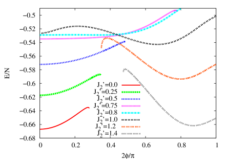
Figure 2: (Color online) Ground-state energy per spin of the spin-1/2 $J_{1}$–$J_{2}^{\prime}$ Hamiltonian of Eq. (1) with $J_{1}=1$, using the LSUB6 approximation of the CCM with the spiral model state, versus the spiral angle $\phi$, for some illustrative values of $J_{2}^{\prime}$ in the range $0\leq J_{2}^{\prime}\leq 1.4$. For $J_{2}^{\prime}\lesssim 0.788$ the minimum is at $\phi=0$ (Néel order), whereas for $J_{2}^{\prime}\gtrsim 0.788$ the minimum occurs at $\phi=\phi_{{\rm LSUB}6}\neq 0$, indicating a phase transition at $J_{2}^{\prime}\approx 0.788$ in this approximation.

show that the Néel model state ($\phi=0$) gives the minimum gs energy for all values of $\kappa<\kappa_{c_{1}}$ where $\kappa_{c_{1}}$ is also dependent on the level of LSUB$n$ approximation, as we also see below in Fig. 3.

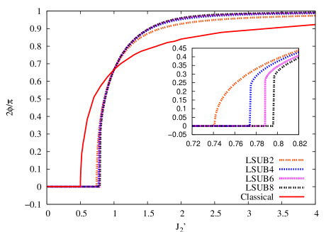
Figure 3: (Color online) The angle $\phi_{{\rm LSUB}n}$ that minimizes the energy $E_{{\rm LSUB}n}(\phi)$ of the spin-1/2 $J_{1}$–$J_{2}^{\prime}$ Hamiltonian Eq. (1) with $J_{1}=1$, in the LSUB$n$ approximations with $n=\{2,4,6,8\}$, using the spiral model state, versus $J_{2}^{\prime}$. The corresponding classical result $\phi_{{\rm cl}}$ is shown for comparison. We find in the LSUB$n$ quantum case with $n>2$ a seemingly first-order phase transition (e.g., for LSUB8 at $J_{2}^{\prime}\approx 0.796$ where $\phi_{{\rm LSUB}8}$ jumps abruptly from zero to about $0.14\pi$), although also see the text for a broader discussion of the nature of the quantum phase transition. By contrast, in the classical case there is a second-order phase transition at $J_{2}^{\prime}=0.5$.

By contrast, for $\kappa>\kappa_{c_{1}}$ the minimum in the energy is found to occur at a value $\phi\neq 0$. If we consider the pitch angle $\phi$ itself as an order parameter (i.e., $\phi=0$ for Néel order and $\phi\neq 0$ for spiral order) a typical scenario for a first-order phase transition would be the appearance of a two-minimum structure for the ground-state energy as a function of $\phi$, exactly as shown in Fig. 2 for the LSUB6 approximation. Very similar curves occur for other LSUB$n$ approximations. If we therefore admit such a scenario, in the typical case one would expect various special points in the transition region, namely the phase transition point $\kappa_{c_{1}}$ itself where the two minima have equal depth, plus one or two instability points $\kappa_{i_{1}}$ and $\kappa_{i_{2}}$ where one or other of the minima (at $\phi=0$ and $\phi\neq 0$ respectively) disappears. In the present case, it is interesting to note that the two points $\kappa_{c_{1}}$ and $\kappa_{i_{2}}$ either coincide exactly or are indistinguishable within the accuracy of our calculations, thereby indicating that the transition at $\kappa_{c_{1}}$ is rather subtle, and perhaps even of second-order rather than first-order type. A close inspection of curves such as those shown in Fig. 2 for the LSUB6 case shows that what happens at this level of approximation is that for $\kappa\lesssim 0.788$ the only minimum in the ground-state energy is at $\phi=0$ (Néel order). As this value is approached asymptotically from below the LSUB6 energy curves become extremely flat near $\phi\neq 0$, indicating the disappearance at $\phi=0$ of the second derivative $d^{2}E/d\phi^{2}$ (and possibly also of one or more of the higher derivatives $d^{n}E/d\phi^{n}$ with $n\geq 3$), as well as of the first derivative $dE/d\phi$. Then, for all values $\kappa\gtrsim 0.788$ the LSUB6 curves develop a secondary minimum at a value $\phi\neq 0$ which is also the global minimum.

The state for $\phi\neq 0$ is believed to be the quantum analog of the classical spiral phase. The fact that Néel order survives beyond the classically stable region is an example of the promotion of collinear order by quantum fluctuations, a phenomenon that has been observed in many other systems (see, e.g., Refs. [Kr:2000, ; Ko:1996, ]). Thus, this collinear ordered state survives for the quantum case into a region where classically it is already unstable. Indeed, one can view this behavior more broadly as another example of the more general phenomenon of order by disorder Vi:1977 that we have briefly alluded to above, in which quantum fluctuations act to select and stabilize an appropriate type of order (that is typically collinear) in the face of classical degeneracy or near-degeneracy.

It is also particularly interesting to note that the crossover from one minimum ($\phi=0$, Néel) solution to the other ($\phi\neq 0$, spiral) appears (except for the LSUB$2$ case) to be quite abrupt (for all other LSUB$n$ cases with even $n>2$) at this point (and see Figs. 2 and 3). Thus, for example, for the LSUB6 case the spiral pitch angle $\phi$ appears to jump discontinuously from a zero value on the Néel side ($\kappa\lesssim 0.788$) to a value of about $0.13\pi$ as the transition point into the spiral phase is crossed. This behavior is a clear first indication of a phase transition. Based on this evidence alone it would also appear that this transition is first-order, by contrast with the second-order nature of its classical counterpart. Such a situation where the quantum fluctuations change the nature of a phase transition qualitatively from a classical second-order type to a quantum first-order type has also been seen previously in the comparable spin-1/2 HAF model that interpolates continuously between the square and honeycomb lattices. Kr:2000 However, due to the extreme insensitivity of the energy to the pitch angle near the phase transition, as discussed above, we cannot rule out a continuous but very steep rise in pitch angle as the transition from the Néel phase into the spiral phase is transversed. All of the available evidence to date indicates that the transition at $\kappa_{c_{1}}$ is subtle and may actually be second-order. Further evidence for the position $\kappa_{c_{1}}$ and nature of the Néel–spiral quantum phase transition also comes from the behavior of the on-site magnetization that we discuss below.

Before doing so, however, we wish to make some further observations on Figs. 2 and 3. We note first from Fig. 3 that in the case $\kappa=1$ ($J_{1}=1,J_{2}^{\prime}=1$), corresponding to the spin-1/2 HAF on the triangular lattice, all of the CCM LSUB$n$ approximations give precisely the classical value $\phi=\frac{\pi}{3}$ for the spiral angle, which corresponds to the correct 120^∘ three-sublattice ordering. The fact that all LSUB$n$ approximations give exactly this value is a consequence of us defining the LSUB$n$ configurations on the triangular lattice (rather than the square lattice), and is a reflection of the exact triangular symmetry that is thereby preserved by our approximations. It is also interesting to note that for values of $\kappa>1$ the quantum spiral angle $\phi$ approaches the asymptotic ($\kappa\rightarrow\infty$) value of $\frac{\pi}{2}$ much faster than does the classical angle. This is a first indication again, in this limit, of quantum fluctuations favoring collinear order (along the weakly coupled chains in this limit).

We note from Fig. 2 that for certain values of $J_{2}^{\prime}$ (or, equivalently, $\kappa$) CCM solutions at a given LSUB$n$ level of approximation (viz., LSUB$6$ in Fig. 2) exist only for certain ranges of spiral angle $\phi$. For example, for the pure square-lattice HAF ($\kappa=0$) the CCM LSUB$6$ solution based on a spiral model state only exists for $0\leq\phi\lesssim 0.14\pi$. In this case, where the Néel solution is the stable ground state, if we attempt to move too far away from Néel collinearity the CCM equations themselves become “unstable” and simply do not have a real solution. Similarly, we see from Fig. 2 that for $\kappa=1.4$ the CCM LSUB$6$ solution exists only for $0.24\pi\lesssim\phi\leq 0.5\pi$. In this case the stable ground state is a spiral phase, and now if we attempt to move too close to Néel collinearity the real solution terminates.

Such terminations of CCM solutions are very common and are very well documented.Fa:2004 In all such cases a termination point always arises due to the solution of the CCM equations becoming complex at this point, beyond which there exist two branches of entirely unphysical complex conjugate solutions.Fa:2004 In the region where the solution reflecting the true physical solution is real there actually also exists another (unstable) real solution. However, only the (shown) upper branch of these two solutions reflects the true (stable) physicsl ground state, whereas the lower branch does not. The physical branch is usually easily identified in practice as the one which becomes exact in some known (e.g., perturbative) limit. This physical branch then meets the corresponding unphysical branch at some termination point (with infinite slope on Fig. 2) beyond which no real solutions exist. The LSUB$n$ termination points are themselves also reflections of the quantum phase transitions in the real system, and may be used to estimate the position of the phase boundary,Fa:2004 although we do not do so for this first critical point since we have more accurate criteria discussed below.

Thus, in Figs. 4 and 5 we show the CCM results for the gs energy and gs on-site magnetization, respectively, where the helical state has been used as the model state and the angle $\phi$ chosen as described above.

Figure 4: (Color online) Ground-state energy per spin versus $J_{2}^{\prime}$ for the Néel and spiral phases of the spin-1/2 $J_{1}$–$J_{2}^{\prime}$ Hamiltonian of Eq. (1) with $J_{1}=1$. The CCM results using the spiral model state are shown for various LSUB$n$ approximations ($n=\{2,4,6,8\}$) with the spiral angle $\phi=\phi_{{\rm LSUB}n}$ that minimizes $E_{{\rm LSUB}n}(\phi)$. We also show the $n\rightarrow\infty$ extrapolated result from using Eq. (2).

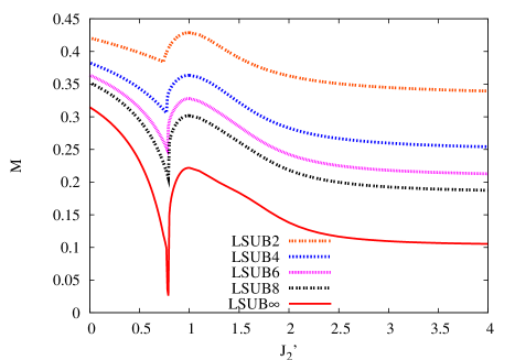
Figure 5: (Color online) Ground-state magnetic order parameter (i.e., the on-site magnetization) versus $J_{2}^{\prime}$ for the Néel and spiral phases of the spin-1/2 $J_{1}$–$J_{2}^{\prime}$ Hamiltonian of Eq. (1) with $J_{1}=1$. The CCM results using the spiral model state are shown for various LSUB$n$ approximations ($n=\{2,4,6,8\}$) with the spiral angle $\phi=\phi_{{\rm LSUB}n}$ that minimizes $E_{{\rm LSUB}n}(\phi)$. We also show the $n\rightarrow\infty$ extrapolated result from using Eq. (3).

For both quantities we show the raw LSUB$n$ data for $n=\{2,4,6,8\}$ and the extrapolated (LSUB$\infty$) results obtained from them by using Eqs. (2) and (3) respectively. Firstly, the gs energy (in Fig. 4) shows signs of a (weak) discontinuity in slope at the critical values $\kappa_{c_{1}}$ discussed above. These values for $\kappa_{c_{1}}$ themselves depend weakly on the approximation level.

Secondly, the gs magnetic order parameter in Fig. 5 shows much stronger and much clearer evidence of a phase transition at the corresponding $\kappa_{c_{1}}$ values previously observed in Fig. 3. The extrapolated value of $M$ shows clearly its steep drop towards a value very close to zero at $\kappa_{c_{1}}=0.80\pm 0.01$, which is hence our best estimate of the phase transition point. From the Néel side ($\kappa<\kappa_{c_{1}}$) the magnetization seems to approach continuously a value $M=0.025\pm 0.025$, whereas from the spiral side ($\kappa>\kappa_{c_{1}}$) there appears to be a discontinuous jump in the magnetization as $\kappa\rightarrow\kappa_{c_{1}}$. The transition at $\kappa=\kappa_{c_{1}}$ thus appears to be (very) weakly first-order but we cannot exclude it being second-order, since we cannot rule out the possibility of a continuous but very steep drop to zero of the on-site magnetization as $\kappa\rightarrow\kappa_{c_{1}}$ from the spiral side of the transition, for the same reasons as enunciated above in connection with our discussion of Fig. 2 and 3. We find no evidence at all for any intermediate phase between the quasiclassical Néel and spiral phases. These results may be compared with those for the same model of Weihong et al.We:1999 who used a linked-cluster series expansion technique. They found that while a nonzero value of the Néel staggered magnetization exists for $0\leq\kappa\lesssim 0.7$, the region $0.7\lesssim\kappa\lesssim 0.9$ has zero on-site magnetization, and for $\kappa\gtrsim 0.9$ they found evidence of spiral order. Nevertheless, their results came with relatively large errors, especially for the spiral phase, and we believe that our own results are probably intrinsically more accurate than theirs.

As a further indication of the accuracy of our results we show in Table 2

Table 2: Ground-state energy per spin and magnetic order parameter (i.e., the on-site magnetization) for the spin-1/2 HAF on the square and triangular lattices. We show CCM results obtained for the $J_{1}$–$J_{2}^{\prime}$ model with $J_{1}>0$, using the spiral model state in various LSUB$n$ approximations defined on the triangular lattice geometry, for the two cases $\kappa\equiv J_{2}^{\prime}/J_{1}=0$ (square lattice HAF, $\phi=0$) and $\kappa=1$ (triangular lattice HAF, $\phi=\frac{\pi}{3}$). We compare our extrapolated ($n\rightarrow\infty$) results using Eqs. (2) and (3) and various sets of LSUB$n$ data with other calculations.

Method	$E/N$	$M$		$E/N$	$M$
	square ($\kappa=0$)			triangular ($\kappa=1$   )
LSUB$2$	-0.64833	0.4207		-0.50290	0.4289
LSUB$3$	-0.64931	0.4182		-0.51911	0.4023
LSUB$4$	-0.66356	0.3827		-0.53427	0.3637
LSUB$5$	-0.66345	0.3827		-0.53869	0.3479
LSUB$6$	-0.66695	0.3638		-0.54290	0.3280
LSUB$7$	-0.66696	0.3635		-0.54502	0.3152
LSUB$8$	-0.66816	0.3524		-0.54679	0.3018
Extrapolations
LSUB$\infty$ a	-0.66978	0.3148		-0.55113	0.2219
LSUB$\infty$ b	-0.66974	0.3099		-0.55244	0.1893
LSUB$\infty$ c	-0.67045	0.3048		-0.55205	0.2085
QMC d,e	-0.669437(5)	0.3070(3)		-0.5458(1)	0.205(10)
SE f,g	-0.6693(1)	0.307(1)		-0.5502(4)	0.19(2)

^a Based on $n=\{2,4,6,8\}$

^b Based on $n=\{4,6,8\}$

^c Based on $n=\{3,5,7\}$

^d QMC (Quantum Monte Carlo) for square latticeSa:1997

^e QMC for triangular latticeCa:1999

^f SE (Series Expansion) for square latticeZh:1991

^g SE for triangular latticeZh:2006

data for the two cases of the spin-1/2 HAF on the square lattice ($\kappa=0$) and on the triangular lattice ($\kappa=1$). For both cases we present our CCM results in various LSUB$n$ approximations (with $2\leq n\leq 8$) based on the triangular lattice geometry using the spiral model state, with $\phi=0$ for the square lattice and $\phi=\frac{\pi}{3}$ for the triangular lattice. Results are given for the gs energy per spin $E/N$, and the magnetic order parameter $M$. We also display our extrapolated ($n\rightarrow\infty$) results using the schemes of Eqs. (2) and (3) with the three data sets $n=\{2,4,6,8\}$, $n=\{4,6,8\}$ and $n=\{3,5,7\}$. The results are seen to be very robust and consistent. For comparison we also show the results obtained for the two lattices using quantum Monte Carlo (QMC) methodsSa:1997 ; Ca:1999 and linked-cluster series expansions.Zh:2006 ; Zh:1991 For the square lattice there is no dynamic frustration and the Marshall-Peierls sign ruleMa:1955 applies, so that the QMC “minus-sign problem” may be circumvented. In this case the QMC resultsSa:1997 are extremely accurate, and indeed represent the best available for the spin-1/2 square-lattice HAF. Our own extrapolated results are in complete agreement with these QMC benchmark results, as found previously (see, e.g., Ref. [Fa:2008, ] and references cited therein), even though the LSUB$n$ configurations are defined here on the triangular lattice geometry. Thus, we note that whereas the individual LSUB$n$ results for the spin-1/2 square-lattice HAF do not coincide with previous results for this model (see, e.g., Ref. [Fa:2008, ]) because previous results have been based on defining the fundamental LSUB$n$ configurations on a square-lattice geometry rather than on the triangular-lattice geometry used here, the corresponding LSUB$\infty$ extrapolations in the two geometries are in complete agreement with each other.

By contrast, the nodal structure of the gs wave function is not exactly known for the spin-1/2 triangular-lattice HAF, and the QMC minus-sign problem cannot now be avoided for such frustrated spin systems. The QMC results shownCa:1999 for the triangular lattice in Table 2 were performed using a Green’s function Monte Carlo method with a fixed-node approximation that was then relaxed in a controlled but approximate way using a stochastic reconfiguration technique. For the triangular lattice case we also show results in Table 2 from a large-scale calculation using a linked-cluster series expansion.Zh:2006 For such frustrated systems this method, along with our CCM, is probably among the most accurate available. We see that in this case our results for the gs energy are in good agreement with the series expansion results, whereas the QMC estimate for the energy is almost certainly too high, and its quoted error hence erroneous. Our best estimate for the sublattice magnetization in this case, $M=0.20\pm 0.02$, is in complete agreement with the best available by all other methods.

The good agreement, both with respect to internal consistency checks using different extrapolations and with respect to other methods, for the gs properties of both the above models, gives us considerable confidence in our results for the spin-1/2 $J_{1}$–$J_{2}^{\prime}$ model for all values of $\kappa\equiv J_{2}^{\prime}/J_{1}$.

We also comment on the $\kappa\rightarrow\infty$ (decoupled spin-1/2 1D HAF chains) limits of Figs. 4 and 5. Firstly, Fig. 4 shows that at large $J_{2}^{\prime}$ the extrapolated energy per spin approaches the value $E/N=-0.4431J_{2}^{\prime}$ which is the same as the exact resultHu:1938 from the Bethe ansatz solution.Be:1931 By contrast, the extrapolated magnetic order parameter at large $J_{2}^{\prime}$ seems to approach a constant value $M\approx 0.10$, by contrast with the exact value of zeroBe:1931 ; Hu:1938 in this limit. We note that the 1D anisotropic $XXZ$ chain with anisotropy parameter $\Delta$ has an essential singularity for $M\rightarrow 0$ at the isotropic point $\Delta\rightarrow 0$ and this is extremely difficult to mimic in any truncated numerical calculation. We note, however, that in the regime $1\lesssim\kappa\lesssim 2$ the order parameter $M$ decreases almost linearly, and if this linear decrease were to be extended $M$ would become zero at a value $\kappa\approx 3.5$.

We turn finally to our CCM results based on the stripe state as CCM gs model state $|\Phi\rangle$. The LSUB$n$ configurations are again defined with respect to the triangular lattice geometry, exactly as before. Results for the gs energy and magnetic order parameter are shown in Figs. 6 and 7 respectively for the collinear stripe phase.

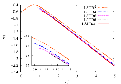
Figure 6: (Color online) Ground-state energy per spin versus $J_{2}^{\prime}$ for the stripe-ordered phase of the spin-1/2 $J_{1}$–$J_{2}^{\prime}$ Hamiltonian of Eq. (1) with $J_{1}=1$. The CCM results using the stripe model state are shown for various LSUB$n$ approximations ($n=\{2,4,6,8\}$). We also show the $n\rightarrow\infty$ extrapolated result from using Eq. (2).

Figure 7: (Color online) Ground-state magnetic order parameter (i.e., the on-site magnetization) versus $J_{2}^{\prime}$ for the stripe-ordered phase of the spin-1/2 $J_{1}$–$J_{2}^{\prime}$ Hamiltonian of Eq. (1) with $J_{1}=1$. The CCM results using the stripe model state are shown for various LSUB$n$ approximations ($n=\{2,4,6,8\}$). We also show the $n\rightarrow\infty$ extrapolated result from using Eq. (3).

They are the precise analogs of Figs. 4 and 5 for the (Néel and) spiral phases. We see from Fig. 6 that some of the LSUB$n$ solutions based on the stripe state show a clear termination point $\kappa_{t}$ of the sort discussed previously, such that for $\kappa<\kappa_{t}$ no real solution for the stripe phase exists. In particular the LSUB$6$ and LSUB$8$ solutions terminate at the values shown in Table 3.

Table 3: The parameters $\kappa_{e}$ (the crossing point of the energy curves for the stripe and spiral phases) and $\kappa_{t}$ (the termination point of the stripe state solution) in various LSUB$n$ approximations defined on the triangular lattice geometry, for the spin-1/2 $J_{1}$–$J_{2}^{\prime}$ model, with $\kappa\equiv J_{2}^{\prime}/J_{1}$, $J_{1}>0$. The “LSUB$\infty$” extrapolations are explained in the text.

LSUB$n$	$J_{2}^{\prime}$
	$\kappa_{e}$	$\kappa_{t}$
LSUB2	$\infty$	-
LSUB4	4.555	(0.880)
LSUB6	3.593	0.970
LSUB8	3.125	1.150
“LSUB$\infty$”	$1.69\pm 0.03$	1.69

As is often the case the LSUB$2$ solution does not terminate, while the LSUB$4$ solution shows a marked change in character around the value $\kappa\approx 0.880$ that is not exactly a termination point (but, probably, rather reflects a crossing with another unphysical solution). In any event, the LSUB$4$ data are not shown below this value in Figs. 6 and 7.

The large $\kappa$ limit of the energy per spin results of Fig. 6 again agrees with the exact 1D chain result of $E/N=-0.4431J_{2}^{\prime}$, just as in Fig. 4 for the spiral phase. However, the most important observation is that for all LSUB$n$ approximations with $n>2$ the curves for the energy per spin of the stripe phase cross with the corresponding curves (i.e., for the same value of $n$) for the energy per spin of the spiral phase at a value that we denote as $\kappa_{e}$. Thus, for $\kappa<\kappa_{e}$ the spiral phase is predicted to be the stable phase (i.e., lies lowest in energy), whereas for $\kappa>\kappa_{e}$ the stripe phase is predicted to be the stable ground state. We thus have a clear first indication of another (first-order) quantum phase transition in the spin-1/2 $J_{1}$–$J_{2}^{\prime}$ model at a value $\kappa=\kappa_{c_{2}}$. Figure 8

Figure 8: (Color online) Difference between the ground-state energies per spin ($e\equiv E/N$) of the spiral and stripe phases ($\Delta e\equiv e^{{\rm spiral}}-e^{{\rm stripe}}$) versus $J_{2}^{\prime}$ for the spin-1/2 $J_{1}$–$J_{2}^{\prime}$ Hamiltonian of Eq. (1) with $J_{1}=1$. The CCM results for the energy difference using the stripe and spiral model states for various LSUB$n$ approximations (n$=\{4,6,8\}$) are shown. We also show the $n\rightarrow\infty$ extrapolated result from using Eq. (2) for the two phases separately.

shows the energy difference between the stripe and spiral states for various LSUB$n$ calculations, and some indicative values near the crossing values $\kappa_{e}$ are also shown in Table 3.

As we remarked in Sec. II, the stripe phase is never the stable classical ground state since it always lies higher in energy than the spiral phase. Indeed, it is easy to show that the classical gs energy per spin, written as $e\equiv E(Ns^{2}J_{2}^{\prime})^{-1}$, has the value $e^{{\rm stripe}}_{{\rm cl}}=-1$ (independent of $J_{1}$) for the stripe phase, and $e^{{\rm spiral}}_{{\rm cl}}=-1-\frac{1}{2}\kappa^{-2}$ for the spiral phase in the regime $\kappa\geq\frac{1}{2}$ where the spiral phase exists classically. Thus, the difference in energy between the two phases classically is $e^{{\rm spiral}}_{{\rm cl}}-e^{{\rm stripe}}_{{\rm cl}}\equiv\Delta e_{{\rm cl}}=-\frac{1}{2}\kappa^{-2}<0$. By contrast, what we have shown at the quantum level is that quantum fluctuations can change the sign of $\Delta e$ at some critical value $\kappa=\kappa_{c_{2}}$ such that the collinear stripe phase becomes stabilized for all $\kappa>\kappa_{c_{2}}$. However, the energy differences $\Delta e$ in this regime are found to be extremely small, as may be seen from Fig. 8,

Table 4: Comparision of the gs energy per spin of the stripe and spiral phases of the spin-$1/2$ $J_{1}$–$J_{2}^{\prime}$ model in various LSUB$n$ approximations ($n=\{2,4,6,8\}$) at some illustrative values of $J_{2}^{\prime}$ (with $J_{1}=1$).

LSUB$n$	$J_{2}^{\prime}$	$E/N$
		stripe	spiral
2	10	-4.167865	-4.168525
4	4.4	-1.927326	-1.927337
4	4.6	-2.014224	-2.014219
4	4.8	-2.101154	-2.101136
6	3.4	-1.508386	-1.508406
6	3.6	-1.595632	-1.595632
6	3.8	-1.682968	-1.682952
8	2.9	-1.295557	-1.295584
8	3.1	-1.382665	-1.382667
8	3.3	-1.469937	-1.469924

and hence the stripe phase is predicted to be very fragile against small perturbations or thermal fluctuations, for example. Nevertheless, we should stress that the LSUB$n$ energy differences displayed in Fig. 8 are well within (by several orders of magnitude) the margins of error in our individual calculations.

Clearly, the LSUB$n$ energy crossing points $\kappa_{e}(n)$ at which $\Delta e_{{\rm LSUB}n}=0$ provide a measure of $\kappa_{c_{2}}$. In the past we have found that a simple linear extrapolation, $\kappa=c_{0}+c_{1}n^{-1}$, yields a good fit to such critical points, and this seems to be the case here too. The corresponding “LSUB$\infty$” estimate from the $\kappa_{e}$ LSUB$n$ data of Table 3 with $n=\{4,6,8\}$ gives an estimate $\kappa_{c_{2}}\approx 1.69\pm 0.03$, where the error is the standard deviation in the fit. A similar linear extrapolation on the LSUB$n$ stripe-phase termination points $\kappa_{t}$ with $n=\{6,8\}$ gives a second estimate $\kappa_{c_{2}}\approx 1.69$, in remarkably good agreement with the first estimate. We note too that we can, of course, also obtain another estimate of $\kappa_{e}$ from the crossing point of the two extrapolated (LSUB$\infty$) gs energy curves for the spiral and stripe-ordered phases (i.e., using Eq. (2) in each case), shown in Figs. 4 and 6 respectively, and it is this LSUB$\infty$ result that is displayed in Fig. 8. Since the two curves cross at such a very shallow angle, and since both curves are extrapolated completely independently of one another, we expect that this estimate for $\kappa_{e}$ is perhaps intrinsically less accurate than the one discussed above. Nevertheless, it is very gratifying that the value so obtained for the crossing point of the two extrapolated (LSUB$\infty$) gs energy curves, namely $\kappa_{e}\approx 2.19$, is rather close to the previous value, considering that the two curves are almost parallel to one another in the crossing region. The difference in the two estimates for $\kappa_{e}$ of about 1.7 and 2.2 is itself an indication of the error in these estimates in this incredibly difficult regime where the two phases lie so close in energy to one another. Nevertheless, we reiterate that the CCM retains sufficient accuracy for both the spiral and stripe phases individually (both in the raw LSUB$n$ data and in the extrapolated LSUB$\infty$ results for each phase) to ensure that, even though the corresponding estimates for the energy difference $\Delta e$ are small in the crossing regime and for values of $\kappa>\kappa_{c}$, they are still sufficiently large to be well within our limits of accuracy.

Finally, from Fig. 7 we see the corresponding results for the magnetic order parameter of the stripe phase. The large-$\kappa$ limit of uncoupled 1D spin-1/2 chains is identical to that for the spiral phase, and hence suffers from the same (known) problem of not giving the correct $M=0$ result in this limit. However at smaller values of $\kappa$ the order parameter decreases and becomes zero at some critical value $\kappa_{m}(n)$ that depends on the LSUB$n$ approximation. The extrapolated ($n\rightarrow\infty$) result obtained in the usual way from Eq. (3) is also shown in Fig. 7 and is seen to become zero at a value $\kappa_{m}\approx 1.43$. Since the phase transition at $\kappa=\kappa_{c_{2}}$ is clearly of first-order type from the energy data, the magnetization data provide us only with an inequality $\kappa_{c_{2}}\geq\kappa_{m}$.

In summary, although it is difficult to put firm error bars on our results for our predicted second critical point, our best current estimate, based on all the above results, is $\kappa_{c_{2}}=1.8\pm 0.4$.

V Discussion and Conclusions

In this paper we have used the CCM to study the influence of quantum fluctuations on the zero-temperature gs phase diagram of a spin-half Heisenberg antiferromagnet, the $J_{1}$–$J_{2}^{\prime}$ model, defined on an anisotropic 2D lattice. We have studied the case where the NN $J_{1}$ bonds are antiferromagnetic ($J_{1}>0$) and the competing $J_{2}^{\prime}\equiv\kappa J_{1}$ bonds have a strength $\kappa$ that varies from $\kappa=0$ (corresponding to the spin-half HAF on the square lattice) to $\kappa\rightarrow\infty$ (corresponding to a set of decoupled spin-half 1D HAF chains), with the spin-half HAF on the triangular lattice as the special case $\kappa=1$ in between the two extremes.

Whereas at the classical level the model has only two stable gs phases, one with Néel order for $\kappa<\kappa_{{\rm cl}}=0.5$ and another with spiral order for $\kappa>\kappa_{{\rm cl}}$, the quantum fluctuations for the spin-half model can stabilize a third non-classical phase with collinear stripe ordering at sufficiently high values of $\kappa$. Thus, we find two quantum phase transitions, both seemingly first-order. The first at $\kappa_{{\rm cl}}=0.80\pm 0.01$ separates a phase with classical Néel ordering for $\kappa<\kappa_{c_{1}}$ from a phase with helical ordering for $\kappa>\kappa_{c_{1}}$. This latter phase includes the case $\kappa=1$ of the spin-half triangular-lattice HAF with the standard 120^∘ three-sublattice quasiclassical ordering. By contrast with the classical second-order transition at $\kappa_{{\rm cl}}=0.5$, the quantum phase transition at $\kappa_{c_{1}}\approx 0.80$ appears to be weakly first-order in nature, although we cannot exclude it from being second-order. The Néel order thus survives into a region $0.5<\kappa<\kappa_{c_{1}}$ where it is classically unstable. This is an example, among many others, of the widely observed phenomenon that quantum fluctuations tend to favor collinear ordering.

A second quantum phase transition is predicted by our calculations to occur at $\kappa_{c_{2}}=1.8\pm 0.4$. It separates the helical phase for $\kappa<\kappa_{c_{2}}$ from a phase with collinear stripe ordering at $\kappa>\kappa_{c_{2}}$. However in this latter region, $\kappa>\kappa_{c_{2}}$, the stripe and spiral phases are extremely close in energy, and hence the stripe phase may be very fragile against external perturbations or thermal fluctuations, for example. The existence of the collinear stripe phase seems to rely again on the fact that quantum fluctuations favor collinear ordering. An alternative, but essentially equivalent, explanation starts by looking at the large-$\kappa$ limit of uncoupled 1D HAF chains, for which all states with spins on different chains orienting randomly with respect to each other are degenerate in energy in the $\kappa\rightarrow\infty$ limit. Then, as the interchain coupling $J_{1}=J_{2}^{\prime}/\kappa$ is slowly increased from zero, what seems to occur is that the relative orientations are locked into collinearity by the familiar phenomenon of order by disorder.Vi:1977 As a somewhat technical aside at this point we note, however, that while the present $J_{1}$–$J_{2}^{\prime}$ model attains (collinear) order from an otherwise disordered set of spin chains, the order by disorder phenomenon seemingly responsible here differs in an important respect from its archetypal realization in the $J_{1}$–$J_{2}$ model. In this latter case each of the inter-penetrating sublattices is characterized by a classical magnetization vector, and the classical disorder emanates from the independence of the energy on the mutual orientation of the magnetization vectors for the two sublattices. By contrast, for the present $J_{1}$–$J_{2}^{\prime}$ model, the corresponding phenomenon is more subtle since the spin chains that now order (collinearly) are themselves quantum-critical. Hence, what is established now is not only that the relative orientations of the magnetizations on different chains become locked into collinear order, but also the very fact that such a classical notion is actually appropriate.

We note that our own calculations are weakest precisely in the $\kappa\rightarrow\infty$ limit where, although our result for the gs energy of the chains is excellent, the subtle quantum-critical ordering of the Bethe ansatz solution that results in the value $M=0$ for the staggered magnetization,Hu:1938 is not exactly reproduced. Nevertheless, with the single exception of our inability to reproduce exactly this very singular and non-analytic result for the on-site magnetization,Hu:1938 the CCM calculations are remarkably robust and accurate over the rest of the parameter space. Thus, our results for the gs energy and on-site magnetization have provided a set of independent checks that lead us to believe that we have a self-consistent and coherent description of this interesting model.

Before concluding we compare our results with those from previous calculations on the same model. The simplest such studies have utilized lowest-order (or linear) spin-wave theory (LSWT)Tr:1999 ; Me:1999 and Schwinger boson mean-field theory (SBMFT).Ga:1993 The independent LSWT calculations of TrumperTr:1999 and Merino et al.Me:1999 both found a continuous second-order phase transition from a Néel-ordered to a spiral-ordered phase at precisely the classical value $\kappa_{c_{1}}=0.5$, at which the magnetization order parameter approaches zero continuously from both sides. Although LSWT is known to give a reasonable description of the spin-1/2 Heisenberg antiferromagnet on both the square lattice ($\kappa=0$) and the triangular lattice ($\kappa=1$), it is clearly unable to model the intermediate regime accurately. This is particularly true around the point of maximum classical frustration at $\kappa=1/2$, for which one fully expects, as mentioned previously, that Néel order is preserved to higher values of $\kappa$ than pertain classically, as found both by earlier more accurate studies, such as those using series expansion (SE) techniques,We:1999 and by us in the present paper.

Similar shortcomings of spin-wave theory (SWT) have been noted by IgarashiIg:1993 in the context of the related spin-1/2 $J_{1}$–$J_{2}$ model on the square lattice, discussed briefly in Sec. I. He showed that whereas its lowest-order version (LSWT) works well when $J_{2}=0$, it consistently overestimates the quantum fluctuations as the frustration $J_{2}/J_{1}$ increases. In particular he showed by going to higher orders in SWT in powers of $1/s$ where $s$ is the spin quantum number and LSWT is the leading order, that the expansion converges reasonably well for $J_{2}/J_{1}\lesssim 0.35$, but for larger values of $J_{2}/J_{1}$, including the point $J_{2}/J_{1}=0.5$ of maximum classical frustration, the series loses stability. He also showed that the higher-order corrections to LSWT for $J_{2}/J_{1}\lesssim 0.4$ make the Néel-ordered phase more stable than predicted by LSWT. He concluded that any predictions from SWT for the spin-1/2 $J_{1}$–$J_{2}$ model on the square lattice are likely to be unreliable for values $J_{2}/J_{1}\gtrsim 0.4$. It is likely that a similar analysis of the SWT results for the present spin-1/2 $J_{1}$–$J_{2}^{\prime}$ model on the square lattice would reveal similar shortcomings of LSWT as the frustration parameter $\kappa\equiv J_{2}^{\prime}/J_{1}$ is increased.

By contrast with the above LSWT results for the spin-1/2 $J_{1}$–$J_{2}^{\prime}$ model on the square lattice, a SBMFT analysisGa:1993 shows a continuous transition from a collinear Néel phase to a spiral phase at a value $\kappa_{c_{1}}\approx 0.6$, but with a non-varnishing magnetization, $M\approx 0.175$, at the critical point. The discrepancy with our own results (viz., $\kappa_{c_{1}}\approx 0.80$ with either a vanishing or very small magnetization, $M\approx 0.025\pm 0.025$, at the critical point) is almost certainly again due to the lowest-order nature of the mean-field approach, and particularly the complete neglect at the SBMFT level of Gaussian fluctuations.

Turning to the second phase transition we note that LSWT predicts that the magnetization in the spiral phase of the present spin-1/2 $J_{1}$–$J_{2}^{\prime}$ model vanishes at a value $\kappa\approx 3.70$. The authors of these resultsTr:1999 ; Me:1999 took that to indicate the possible existence of a disordered phase for $\kappa\gtrsim 3.70$. Even ignoring the probably unreliable nature of LSWT results for such high values of $\kappa$, as noted above, the safer conclusion based on them is that the spiral phase simply becomes unstable for $\kappa\gtrsim 3.70$. Indeed, SWT results are always based on a particular choice of phase, usually based on a classical ($s\rightarrow\infty$) analog, just as are our own CCM calculations. In both cases the vanishing of an order parameter only signals a phase transition to another state, but in the absence of another calculation based on another (classical) hypothesized phase, no conclusion about the adjacent phase can be drawn. It is precisely such an additional calculation based on a stripe-ordered phase that has been done in the present work, which has shown the onset of this phase (at a lower-energy than the spiral phase) for $\kappa>\kappa_{c_{2}}\approx 1.8\pm 0.4$. No such calcultions were attempted in either the LSWTTr:1999 ; Me:1999 or the SBMFTGa:1993 cases, and hence no direct comparison can be drawn with own results for this second phase transition, except to say that the LSWT result with its expected uncertainties discussed above is not incompatible with our own conclusions.

As has been noted elsewhere,Bi:2008_JPCM high-order CCM results of the sort presented here are believed to be among the best available for such highly frustrated spin-lattice models. Many previous applications of the CCM to unfrustrated spin models have given excellent quantitative agreement with other numerical methods (including exact diagonalization (ED) of small lattices, quantum Monte Carlo (QMC), and series expansion techniques). A typical example is the spin-half HAF on the square lattice, which is the $\kappa=0$ limit of the present model (and see Table 2). It is interesting to compare for this $\kappa=0$ case, where comparison can be made with QMC results, the present CCM extrapolations of the LSUB$n$ data for the infinite lattice to the $n\rightarrow\infty$ limit and the corresponding QMC or ED extrapolations for the results obtained for finite lattices containing $N$ spins that have to be carried out to give the $N\rightarrow\infty$ limit. Thus, for the spin-1/2 HAF on the square lattice the “distance” between the CCM results for the ground-state energy per spinFa:2008 at the LSUB8 (LSUB10) level and the extrapolated LSUB$\infty$ value is approximately the same as the distance of the corresponding QMC resultRu:1992 for a lattice of size $N=12\times 12$ ($N=16\times 16$) from its $N\rightarrow\infty$ limit. The corresponding comparison for the magnetic order parameter $M$ is even more striking. Thus even the CCM LSUB6 result for $M$ is closer to the LSUB$\infty$ limit than any of the QMC results for $M$ for lattices of $N$ spins are to their $N\rightarrow\infty$ limit for all lattices up to size $N=16\times 16$, the largest for which calculations were undertaken.Ru:1992 Such comparisons show, for example, that even though the “distance” between our LSUB$n$ data points for $M$ and the extrapolated ($n\rightarrow\infty$) LSUB$\infty$ result shown in Fig. 5 may, at first sight, appear to be large, they are completely comparable to or smaller than those in alternative methods (where they can be applied). Furthermore, where such alternative methods can be applied, as for the spin-1/2 HAF on the square lattice, the CCM results are in complete agreement with them.

By contrast, for frustrated spin-lattice models in two dimensions both the QMC and ED techniques face formidable difficulties. These arise in the former case due to the “minus-sign problem” present for frustrated systems when the nodal structure of the gs wave function is unknown, and in the latter case due to the practical restriction to relatively small lattices imposed by computational limits. The latter problem is exacerbated for incommensurate phases, and is compounded due to the large (and essentially uncontrolled) variation of the results with respect to the different possible shapes of clusters of a given size.

Thus, for highly frustrated spin-lattice models like the present $J_{1}$–$J_{2}^{\prime}$ model, the best alternative numerical method to the CCM is the linked-cluster series expansion (SE) technique.We:1999 ; Pa:2008 ; He:1990 ; Ge:1990 ; Ge:1996 The SE technique has also been applied to the present model.We:1999 ; Pa:2008 The earlier studyWe:1999 mainly dealt with the Néel and spiral phases. Unlike in that work we find no evidence at all for an intermediate (dimerized) phase between the Néel and spiral phases in the parameter regime $0.7\lesssim\kappa\lesssim 0.9$. The very recent SE studyPa:2008 was motivated by the prediction of Starykh and BalentsSt:2007 for the existence of a stable collinear stripe-ordered gs phase for values of $\kappa$ above some critical value that they did not calculate. The SE study showed that although the collinear stripe phase was stabilized for large values of $\kappa$ relative to the classical result, nevertheless in their calculations the non-collinear helical phase was still always lower in energy. Hence, they could not confirm the existence of the stripe-ordered phase. They concluded by suggesting that further unbiased ways of studying the competition between the spiral and stripe phases would be useful. We believe that the present CCM calculations provide exactly such unbiased results, which now do indeed appear to confirm the prediction of Starykh and Balents.

We end by remarking that it would also be of interest to repeat the present study for the case of the spin-one $J_{1}$–$J_{2}^{\prime}$ model. The calculations for this case are more demanding due to an increase at a given LSUB$n$ level of approximation in the number of fundamental configurations retained in the CCM correlation operators. Nevertheless, we hope to be able to report results for this system in the future.

References

- (1) S. Sachdev, in Low Dimensional Quantum Field Theories for Condensed Matter Physicists, edited by Y. Lu, S. Lundqvist, and G. Morandi (World Scientific, Singapore 1995).
- (2) J. Richter, J. Schulenburg, and A. Honecker, in Quantum Magnetism, Lecture Notes in Physics Vol. 645, edited by U. Schollwöck, J. Richter, D.J.J. Farnell, and R.F. Bishop, (Springer-Verlag, Berlin, 2004), p.85.
- (3) G. Misguich and C. Lhuillier, in Frustrated Spin Systems, edited by H.T. Diep (World Scientific, Singapore, 2005), p.229.
- (4) R. F. Bishop, P. H. Y. Li, R. Darradi, and J. Richter, J. Phys.: Condens. Matter 20, 255251 (2008).
- (5) R. F. Bishop, P. H. Y. Li, R. Darradi, J. Schulenburg, and J. Richter, Phys. Rev. B 78, 054412 (2008).
- (6) C. J. Gazza and H. A. Ceccatto, J. Phys.: Condens. Matter 5, L135 (1993).
- (7) A. E. Trumper, Phys. Rev. B 60, 2987 (1999).
- (8) J. Merino, R. H. McKenzie, J. B. Marston, and C. H. Chung, J. Phys.: Condens. Matter 11, 2965 (1999).
- (9) Zheng Weihong, R. H. McKenzie, and R. R. P. Singh, Phys. Rev. B 59, 14367 (1999).
- (10) O. A. Starykh and L. Balents, Phys. Rev. Lett. 98, 077205 (2007).
- (11) T. Pardini and R. R. P. Singh, Phys. Rev. B 77, 214433 (2008).
- (12) D. J. J. Farnell, R. F. Bishop, and K. A. Gernoth, Phys. Rev. B 63, 220402(R) (2001).
- (13) S. E. Krüger, J. Richter, J. Schulenburg, D. J. J. Farnell, and R. F. Bishop, Phys. Rev. B 61, 14607 (2000).
- (14) D. Schmalfusz, R. Darradi, J. Richter, J. Schulenburg, and D. Ihle, Phys. Rev. Lett. 97, 157201 (2006).
- (15) H. Kino and H. Fukuyama, J. Phys. Soc. Japan 65, 2158 (1996); R. H. McKenzie, Comments Condens. Matter Phys. 18, 309 (1998).
- (16) R. Coldea, D. A. Tennant, R. A. Cowley, D. F. McMorrow, B. Dorner, and Z. Tylczynski, Phys. Rev. Lett. 79, 151 (1997).
- (17) H. A. Bethe, Z. Phys. 71, 205 (1931).
- (18) J. Villain, J. Phys. (Paris) 38, 385 (1977); J. Villain, R. Bidaux, J. P. Carton, and R. Conte, ibid. 41, 1263 (1980); E. Shender, Sov. Phys. JETP 56, 178 (1982).
- (19) R. F. Bishop, Theor. Chim. Acta 80, 95 (1991).
- (20) R. F. Bishop, in Microscopic Quantum Many-Body Theories and Their Applications, edited by J. Navarro and A. Polls, Lecture Notes in Physics 510 (Springer-Verlag, Berlin, 1998), p.1.
- (21) D. J. J. Farnell and R. F. Bishop, in Quantum Magnetism, edited by U. Schollwöck, J. Richter, D. J. J. Farnell, and R. F. Bishop, Lecture Notes in Physics 645 (Springer-Verlag, Berlin, 2004), p.307.
- (22) C. Zeng, D. J. J. Farnell, and R. F. Bishop, J. Stat. Phys. 90, 327 (1998).
- (23) R. Darradi, J. Richter, and D. J. J. Farnell, Phys. Rev. B 72, 104425 (2005).
- (24) We use the program package “Crystallographic Coupled Cluster Method” (CCCM) of D. J. J. Farnell and J. Schulenburg, see http://www-e.uni-magdeburg.de/jschulen/ccm/index.html.
- (25) D. J. J. Farnell and R. F. Bishop, Int. J. Mod. Phys. B 22, 3369 (2008).
- (26) P. M. Morse and H. Feshbach, Methods of Theoretical Physics, Part II (McGraw-Hill, New York, 1953).
- (27) H. Kontani, M. E. Zhitomirsky, and K. Ueda, J. Phys. Soc. Jpn. 65, 1566 (1996).
- (28) A. W. Sandvik, Phys. Rev. B 56, 11678 (1997).
- (29) L. Capriotti, A. E. Trumper, and S. Sorella, Phys. Rev. Lett. 82, 3899 (1999).
- (30) Zheng Weihong, J. Oitmaa, and C. J. Hamer, Phy. Rev. B 43, 8321 (1991).
- (31) W. Zheng, J. O. Fjaerestad, R. R. P. Singh, R. H. McKenzie, and R. Coldea, Phys. Rev. B 74, 224420 (2006).
- (32) W. Marshall, Proc. R. Soc. London, Ser. A 232, 48 (1955).
- (33) L. Hulthén, Ark. Mat. Astron. Fys. A 26 (No. 11), 1 (1938); R. Orbach, Phys. Rev. 112, 309 (1958); C. N. Yang and C. P. Yang, Phys. Rev. 150, 321 (1966); 150, 327 (1966); R. J. Baxter, J. Stat. Phys. 9, 145 (1973).
- (34) J. Igarashi, J. Phys. Soc. Jpn. 62, 4449 (1993).
- (35) K. J. Runge, Phys. Rev. B 45, 7229 (1992); 12292 (1992).
- (36) H. X. He, C. J. Hamer, and J. Oitmaa, J. Phys. A 23, 1775 (1990).
- (37) M. P. Gelfand, R. R. P. Singh, and D. A. Huse, J. Stat. Phys. 59, 1093 (1990).
- (38) M. P. Gelfand, Solid State Commun. 98, 11 (1996).