Effective Field Theories and Matching for Codimension-2 Branes

Abstract:

It is generic for the bulk fields sourced by branes having codimension two and higher to diverge at the brane position, much as does the Coulomb potential at the position of its source charge. This complicates finding the relation between brane properties and the bulk geometries they source. (These complications do not arise for codimension-1 sources, such as in RS geometries, because of the special properties unique to codimension one.) Understanding these relations is a prerequisite for phenomenological applications involving higher-codimension branes. Using codimension-2 branes in extra-dimensional scalar-tensor theories as an example, we identify the classical matching conditions that relate the near-brane asymptotic behaviour of bulk fields to the low-energy effective actions describing how space-filling codimension-2 branes interact with the surrounding extra-dimensional bulk. We do so by carefully regulating the near-brane divergences, and show how these may be renormalized in a general way. Among the interesting consequences is a constraint relating the on-brane curvature to its action, that is the codimension-2 generalization of the well-known modification of the Friedmann equation for codimension-1 branes. We argue that its interpretation within an effective field theory framework in this case is as a relation $4\pi{U_{2}}\simeq\kappa^{2}\left({{T_{2}}}^{\prime}\right)^{2}$ between the codimension-2 brane tension, ${T_{2}}(\phi)$, and its contribution to the low-energy on-brane effective potential, ${U_{2}}(\phi)$. This relation implies that any dynamics that minimizes a brane contribution to the on-brane curvature automatically also minimizes its couplings to the extra-dimensional scalar.

1 Introduction

The study of codimension-1 branes is very well developed, largely due to the recognition [1] that the warping induced by branes can provide new ways to generate hierarchies. Much less is known about the interactions of higher codimension branes with their environments. But systems with only one codimension are not representative of those having more, and the absence of such studies is likely to strongly bias our understanding of the kinds of physics to which branes can lead [2].

There is a good reason why such studies have not been done. The problem is that (unlike codimension one) for generic codimension the fields sourced by a brane typically diverge at the brane position [3] — indeed the Coulomb potential outside a point charge in 3 spatial dimensions provides a familiar case in point. Such divergences complicate the extraction of useful consequences of brane-bulk interactions, because these often require knowing how the properties of the bulk fields are related to the choices made about the brane-localized physics. Examples of questions that hinge on this kind of connection arise in brane cosmology [4], where one wishes to know how a given energy density and pressure on the brane interacts with the time-dependent extra-dimensional cosmological spacetime, or in particle phenomenology [5]. The connection is also crucial for attempts to use extra dimensions to address the cosmological constant problem [6, 7, 8, 9, 10], since these hinge on understanding the connection between bulk curvatures and radiative corrections on the brane.

In this paper our goal is to develop tools to remedy this situation, adapted for studying the fields sourced by $d$-dimensional space-filling branes sitting within a ($D=d+2$)-dimensional spacetime. Such codimension-2 branes provide the simplest possible laboratory to study the problem of how branes generically interact with their surrounding bulk, and are likely much more representative of the generic higher-codimension situation than are the codimension-1 systems presently being studied. Of special interest is the case where $d=4$, which describes 3-branes sitting within a 6-dimensional spacetime.

We attain this goal by identifying which features of the bulk fields are directly dictated by the branes, and showing precisely how these features depend on the brane action. What we find resembles what one would expect based on the electrodynamics of charge distributions situated within an extra-dimensional bulk: the field behaviour very near a branes is directly governed by that brane’s properties, while overall issues like equilibrium or stability depend on the global properties of all of the branes taken together.

More precisely, the success of our analysis relies on there being a large hierarchy between the small size, $r_{b}$, of the source distribution, compared with the large size, $L$, over which the external field of interest varies. In the electrostatic analogy it is the existence of distances $r$ satisfying $r_{b}\ll r\ll L$ that allows the use of a multipole expansion to relate powers of $r_{b}/r$ to various moments of the source distribution at distances much smaller than the scale, $L$. We assume a similar hierarchy exists in the case of gravitating codimension-2 branes, where $r_{b}$ is of order whatever physics governs the branes’ microscopic structure, while $L$ is more characteristic of the curvature or volume of the geometry transverse to the branes.

Mathematically, we identify the matching conditions that relate the action of the effective field theory governing the low-energy properties of the brane with the asymptotic near-brane properties of the bulk fields they source. These provide the analogue for higher codimension of the well-known Israel junction conditions [11] that determine the matching of codimension-1 branes to their adjacent bulk geometries. We derive these conditions by regularizing the codimension-2 brane by replacing it with an infinitesimal codimension-1 brane that encircles the position of the codimension-2 object of interest. This allows the connection between brane and bulk to be obtained explicitly using standard jump conditions at this codimension-1 position. We then show how the dimensionally reduced codimension-2 action obtained from this regularized brane is related to the derivatives of the bulk fields in the near-brane limit. Finally, we show how to define a renormalized brane action that gives finite results as the size of the regularizing codimension-1 brane shrinks to zero. We derive RG equations for this action and show that they agree with those obtained in special cases by earlier authors using graphical methods.

Along the way we derive a constraint that directly relates the on-brane curvature to the brane action, that generalized to higher codimension the well-known modifications to the Friedmann equation for codimension-1 branes. However we argue that in the limit of a very small brane this equation is better understood as a condition that dynamically determines the size of the regulating codimension-1 brane as a function of the observable fields in the problem, rather than as a direct constraint on the on-brane curvature (since its curvature dependence arises to subleading order in the low-energy expansion).

For codimension-2 branes the main consequence of this constraint is instead to directly relate the codimension-2 brane tension, ${T_{2}}(\phi)$, to the brane contribution, ${U_{2}}(\phi)$, to the effective potential that governs its contribution to the on-brane curvature. Working perturbatively in the bulk gravitational coupling, $\kappa^{2}$, the relation becomes $4\pi{U_{2}}\simeq\kappa^{2}\left({{T_{2}}}^{\prime}\right)^{2}$. A remarkable consequence of this line or argument is the observation that any dynamics that allows the bulk scalar field, $\phi$, to adjust its value at the brane position to minimize its contribution to the on-brane curvature automatically also minimizes its coupling to the codimension-2 brane tension (and vice versa).

We organize our presentation as follows. First, in §2, we review the action and field equations for scalar-tensor theory in $D=d+2$ dimensions. We also summarize the most general solutions to these equations in the limit that the bulk scalar potential vanishes, which typically govern the near-brane asymptotics of the bulk configurations. This allows us to display the singularities these solutions have as they approach these sources. §3 then describes the codimension-1 regularization procedure for dealing with these singularities, together with the implications of the Israel junction conditions. §4 then defines the codimension-2 effective actions for this system, and how they relate to the asymptotic near-brane behaviour of the bulk fields. Finally, §5 shows how to renormalize the near-brane divergences. Our conclusions are summarized in §6.

2 The Bulk

We illustrate the logic of our construction using a simple higher-dimensional scalar-tensor theory, whose properties we now briefly describe.

2.1 Field equations

Consider therefore the following bulk action, describing the couplings between the extra-dimensional Einstein-frame metric, $g_{{\scriptscriptstyle M}{\scriptscriptstyle N}}$, and a real scalar field, $\phi$, in $D=d+2$ spacetime dimensions:

$$S_{B}=-\int\mathrm{d}^{D}x\sqrt{-g}\;\left\{\frac{1}{2\kappa^{2}}\,g^{{\scriptscriptstyle M}{\scriptscriptstyle N}}\Bigl{(}{\cal R}_{{\scriptscriptstyle M}{\scriptscriptstyle N}}+\partial_{\scriptscriptstyle M}\phi\,\partial_{\scriptscriptstyle N}\phi\Bigr{)}+V(\phi)\right\}\,,$$ (1)

where ${\cal R}_{{\scriptscriptstyle M}{\scriptscriptstyle N}}$ denotes the Ricci tensor built from $g_{{\scriptscriptstyle M}{\scriptscriptstyle N}}$. The bulk field equations obtained from this action are

$$\Box\phi-\kappa^{2}\,V^{\prime}(\phi) = 0$$

$${\cal R}_{{\scriptscriptstyle M}{\scriptscriptstyle N}}+\partial_{\scriptscriptstyle M}\phi\,\partial_{\scriptscriptstyle N}\phi+\frac{2\kappa^{2}}{d}\,V\,g_{{\scriptscriptstyle M}{\scriptscriptstyle N}} = 0\,.$$ (2)

Assume, for simplicity, a metric of the form

$$\mathrm{d}s^{2} = \mathrm{d}\rho^{2}+\hat{g}_{mn}\,\mathrm{d}x^{m}\,\mathrm{d}x^{n}$$

$$= \mathrm{d}\rho^{2}+e^{2B}\,\mathrm{d}\theta^{2}+\check{g}_{\mu\nu}\,\mathrm{d}x^{\mu}\,\mathrm{d}x^{\nu}$$

$$= \mathrm{d}\rho^{2}+e^{2B}\,\mathrm{d}\theta^{2}+e^{2W}g_{\mu\nu}\,\mathrm{d}x^{\mu}\,\mathrm{d}x^{\nu}\,,$$

where $\theta\simeq\theta+2\pi$ is an angular coordinate, $B$ and $W$ are functions of $\rho$ only, and $g_{\mu\nu}$ is a maximally symmetric Minkowski-signature metric depending only on $x^{\mu}$. The bulk Ricci tensor then becomes

$${\cal R}_{\mu\nu} = \left\{\frac{\check{R}}{d}+W^{\prime\prime}+d\,(W^{\prime})^{2}+W^{\prime}B^{\prime}\right\}\,\check{g}_{\mu\nu}$$

$${\cal R}_{\theta\theta} = \Bigl{\{}B^{\prime\prime}+(B^{\prime})^{2}+d\,W^{\prime}B^{\prime}\Bigr{\}}\,\check{g}_{\theta\theta}$$ (4)

$${\cal R}_{\rho\rho} = d\,\Bigl{\{}W^{\prime\prime}+(W^{\prime})^{2}\Bigr{\}}+B^{\prime\prime}+(B^{\prime})^{2}\,.$$

so if $\phi=\phi(\rho)$ we obtain the following bulk field equations:

$$\phi^{\prime\prime}+\Bigl{\{}d\,W^{\prime}+B^{\prime}\Bigr{\}}\phi^{\prime}-\kappa^{2}V^{\prime} = 0\quad\hbox{($\phi$)}$$

$$\frac{\check{R}}{d}+W^{\prime\prime}+d\,(W^{\prime})^{2}+W^{\prime}B^{\prime}+\frac{2\kappa^{2}V}{d} = 0\quad\hbox{($\mu\nu$)}$$

$$B^{\prime\prime}+(B^{\prime})^{2}+d\,W^{\prime}B^{\prime}+\frac{2\kappa^{2}V}{d} = 0\quad\hbox{($\theta\theta$)}$$

$$d\,\Bigl{\{}W^{\prime\prime}+(W^{\prime})^{2}\Bigr{\}}+B^{\prime\prime}+(B^{\prime})^{2}+(\phi^{\prime})^{2}+\frac{2\kappa^{2}V}{d} = 0\quad\hbox{($\rho\rho$)}\,.$$ (5)

In these equations primes indicate differentiation with respect to the natural argument (i.e. $\mathrm{d}/\mathrm{d}\phi$ for $V(\phi)$, but $\mathrm{d}/\mathrm{d}\rho$ for $W(\rho)$, etc.).

The special case $V=0$

The case $V=0$ is of special interest for several reasons. First, as we see explicitly below, the field equations may in this case be explicitly integrated for the axially symmetric ansatz given above. Second, these $V=0$ solutions often capture the near-brane behaviour of the bulk fields even when $V$ is nonzero, since in this limit the potential term is often subdominant to others in the field equations.

Two classical symmetries of the field equations also emerge when $V=0$. The first of these is the axion symmetry, for which the action is unchanged under the replacement

$$\phi\to\phi+\zeta\,,$$ (6)

where $\zeta$ is an arbitrary constant and $g_{{\scriptscriptstyle M}{\scriptscriptstyle N}}$ is held fixed. The second follows from the action’s scaling property $S_{\scriptscriptstyle B}\to\lambda^{d}S_{\scriptscriptstyle B}$ under the replacement

$$g_{{\scriptscriptstyle M}{\scriptscriptstyle N}}\to\lambda^{2}g_{{\scriptscriptstyle M}{\scriptscriptstyle N}}\,,$$ (7)

with constant $\lambda$ and $\phi$ held fixed. Both of these symmetries take solutions of the classical field equations into distinct new solutions of the same equations.

2.2 Axisymmetric bulk solutions

The bulk field equation can be integrated to obtain the general solution in the special case $V=0$, and we collect these solutions in this section. As discussed above, these solutions are also relevant when $V\neq 0$, since even in this case they can capture the asymptotic behavior of bulk solutions very near the branes which source them.

When $V=0$ (or when $V$ is minimized at $V=0$) a trivial solution is $\phi^{\prime}=W^{\prime}=0$ and $g_{\mu\nu}=\eta_{\mu\nu}$, but $e^{B}=\alpha\rho$. The constant $\alpha$ can be absorbed by re-scaling it into the coordinate $\theta$, but only at the expense of changing its periodicity to $\theta\simeq\theta+2\pi\alpha$, showing that this solution corresponds to flat space (in cylindrical coordinates) when $\alpha=1$, or a cone (with conical singularity at $\rho=0$ and defect angle $2\pi\delta$, with $\delta=1-\alpha$) if $\alpha\neq 1$.

The general solution to the dilaton and Einstein equations (see Appendix A for details) when $V=0$ is

$$e^{\phi}=e^{\phi_{0}}\left(\frac{r}{r_{0}}\right)^{p_{\phi}}\,,\quad e^{B}=e^{B_{0}}\left(\frac{r}{r_{0}}\right)^{p_{\scriptscriptstyle B}}\,,$$ (8)

and

$$e^{(d-1)W}=\frac{(r_{0}/l_{\scriptscriptstyle W})^{\Omega}+(l_{\scriptscriptstyle W}/r_{0})^{\Omega}}{(r/l_{\scriptscriptstyle W})^{\Omega}+(l_{\scriptscriptstyle W}/r)^{\Omega}}\left(\frac{r_{0}}{r}\right)^{p_{\scriptscriptstyle B}}\,e^{(d-1)W_{0}}\,,$$ (9)

where

$$\Omega^{2}=p_{\scriptscriptstyle B}^{2}+p_{\phi}^{2}\left(\frac{d-1}{d}\right)\,,$$ (10)

and we may take the positive root without loss of generality. The freedom to re-scale $x^{\mu}$ allows us to shift $W_{0}$ arbitrarily, and re-scalings of $r$ allow any value to be chosen for $r_{0}$, leaving five quantities $l_{\scriptscriptstyle W}/r_{0}$, $\phi_{0}$, $B_{0}$, $p_{\phi}$ and $p_{\scriptscriptstyle B}$ as the remaining integration constants. The radial coordinate, $r$, used to solve the equations is related to the radial proper distance, $\rho$, by

$$\frac{\mathrm{d}r}{r}=\xi\,e^{-B-d\,W}\,\mathrm{d}\rho\,,$$ (11)

for arbitrary constant $\xi$.

The curvature scalar in the brane directions is given in terms of the above constants by

$$R=\frac{4d\xi^{2}\Omega^{2}}{(d-1)\,r_{0}^{2}}\;\left[\left(\frac{r_{0}}{l_{\scriptscriptstyle W}}\right)^{\Omega}+\left(\frac{l_{\scriptscriptstyle W}}{r_{0}}\right)^{\Omega}\right]^{-2}e^{-2(d-1)W_{0}}\geq 0\,.$$ (12)

Notice that the curvature obtained is strictly non-negative (corresponding in our conventions to flat or anti-de Sitter geometries), in agreement with general no-go arguments for finding de Sitter solutions in higher-dimensional supergravity.

A key feature of these solutions is the singularities they generically display as $r\to 0$ and $r\to\infty$, which we interpret as being due to the presence there of source branes having dimension $d=D-2$. This divergent near-brane behaviour is an important departure from the codimension-one case. Furthermore, even though these asymptotic near-brane forms are derived using $V=0$, the singular behaviour given above often provides a good approximation in the near-brane limit even for nonzero $V$. To see why, consider the example of a potential of the form $V(\phi)=V_{0}\,e^{\lambda\phi}$. Evaluated at the solution of eq. (17), this gives the following contributions to the field equations

$$\kappa^{2}V^{\prime}\propto\lambda\kappa^{2}V\propto\lambda r^{\lambda p_{\phi}}\propto\lambda\rho^{\zeta}\,,$$ (13)

for calculable $\zeta$. The main point is that this often represents a subdominant contribution to equations eqs. (2.1) as $\rho\to 0$ near the brane, provided $\zeta>-2$, since the other terms in these equations vary like $\partial_{\rho}^{2}\phi\propto 1/\rho^{2}$.

Special Cases

There are a number of special cases that are of particular interest in what follows.

Conical Singularity:

If we wish to avoid a curvature singularity at $r=0$ we must take $p_{\phi}=0$ and so $p_{\scriptscriptstyle B}=\Omega:=p$, in which case $\phi=\phi_{0}$ and $e^{B}=e^{B_{0}}(r/r_{0})^{p}$. The warp factor then becomes

$$e^{(d-1)W}=\left(\frac{r_{0}^{2p}+l_{\scriptscriptstyle W}^{2p}}{r^{2p}+l_{\scriptscriptstyle W}^{2p}}\right)e^{(d-1)W_{0}}\,,$$ (14)

where $r_{0}$ is an arbitrary point where the metric functions are assumed known: $B(r_{0})=B_{0}$ and $W(r_{0})=W_{0}$. The proper distance, $\rho$, is then related to $r$ by

$$\xi\,{\hbox{d}}\rho=e^{B_{0}+dW_{0}}\left(\frac{r}{r_{0}}\right)^{p}\left(\frac{r_{0}^{2p}+l_{\scriptscriptstyle W}^{2p}}{r^{2p}+l_{\scriptscriptstyle W}^{2p}}\right)^{d/(d-1)}\frac{{\hbox{d}}r}{r}\,,$$ (15)

which shows that $p\,\xi\rho=e^{B_{0}+dW_{0}}\left[1+(r_{0}/l_{\scriptscriptstyle W})^{2p}\right]^{d/(d-1)}(r/r_{0})^{p}+{\cal O}\left(r^{3p}\right)$ near $r=0$, and so $e^{B}=\alpha\rho+{\cal O}(\rho^{3})$ with $\alpha=p\,\xi e^{-dW_{0}}\left[1+(r_{0}/l_{\scriptscriptstyle W})^{2p}\right]^{-d/(d-1)}$.

The curvature similarly reduces to

$$R = \frac{4d\,p^{2}\xi^{2}}{(d-1)\,r_{0}^{2}}\,\left(\frac{r_{0}}{l_{\scriptscriptstyle W}}\right)^{2p}\left[1+\left(\frac{r_{0}}{l_{\scriptscriptstyle W}}\right)^{2p}\right]^{-2}e^{-2(d-1)W_{0}}$$ (16)

$$= \frac{4d\,\alpha^{2}}{(d-1)\,r_{0}^{2}}\,\left(\frac{r_{0}}{l_{\scriptscriptstyle W}}\right)^{2p}\left[1+\left(\frac{r_{0}}{l_{\scriptscriptstyle W}}\right)^{2p}\right]^{2/(d-1)}e^{2W_{0}}\,.$$

In general, this geometry has a conical singularity at $\rho=0$, whose defect angle is $2\pi\delta=2\pi(1-\alpha)$. When $\alpha=1$ it is instead purely a coordinate singularity, which requires $p\,\xi=e^{dW_{0}}\left[1+\left(r_{0}/l_{\scriptscriptstyle W}\right)^{2p}\right]^{d/(d-1)}$.

Flat Brane Geometries:

As shown in more detail in Appendix A when the induced brane geometry is flat ($R=0$), the solutions have a simple form when written in terms of $\rho$:

$$e^{\phi}=e^{\phi_{0}}\left(\frac{\rho}{\rho_{0}}\right)^{\gamma}\,,\quad e^{B}=\alpha\,\rho_{0}\left(\frac{\rho}{\rho_{0}}\right)^{\beta}\quad\hbox{and}\quad e^{W}=e^{W_{0}}\left(\frac{\rho}{\rho_{0}}\right)^{\omega}\,,$$ (17)

where the powers satisfy

$$d\,\omega^{2}+\beta^{2}+\gamma^{2}=d\,\omega+\beta=1\,.$$ (18)

In terms of these constants, the trivial solution given above corresponds to the choices $\omega=\gamma=0$ and $\beta=1$. For more general powers the bulk geometry potentially has singularities at $\rho=0$ and at $\rho\to\infty$, which we interpret as being due to the presence there of codimension-2 branes. Several special subcases are worth identifying.

• Conical singularity: The singularity of the bulk geometry at $\rho=0$ is a conical singularity (as opposed to a curvature singularity), if and only if $\beta=1$. In this case eqs. (18) imply $\omega=\gamma=0$, implying $\phi$ and $W$ are constant and $e^{B}=\alpha\,\rho$. This corresponds to the limit $l_{\scriptscriptstyle W}\to\infty$ of the previous example, and as before the conical defect angle, $2\pi\delta$, satisfies $\delta=1-\alpha$.

• Constant dilaton: The scalar $\phi$ does not vary across the extra dimensions if and only if $\gamma=0$, in which case eqs. (18) admit two solutions for $\omega$ and $\beta$: ($i$) the conical solution just discussed, $\omega=0$ and $\beta=1$; or ($ii$) the curved geometry with $\omega=2/(d+1)$ and $\beta=-(d-1)/(d+1)$. Notice that negative $\beta$ implies the circumferences of circles in the extra dimensions having radius $\rho$ decreases with increasing $\rho$ rather than increasing.

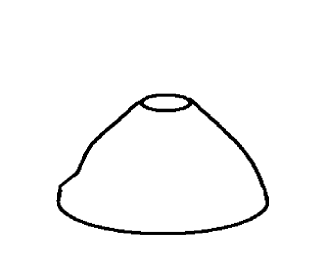
Figure 1: A cartoon of the near-brane cap geometry.

3 The Codimension-One Crutch

We turn now to the problem of establishing how the asymptotic features of the singular near-brane bulk fields are related to the properties of the effective codimension-2 brane which does the sourcing. Experience with the related problem of finding the electrostatic field sourced by a localized charge distribution, we expect to find the near-brane power-law behaviour of the bulk field to be related to the physical properties of the brane.

A trick for finding this connection between a small source brane and the bulk field to which it gives rise involves resolving the codimension-2 singularity in terms of a codimension-1 brane having a very small proper circumference [16, 17]. For instance for the singularity near $\rho=0$, we replace the geometry for $\rho<\rho_{b}$ with a new smooth geometry (see Fig. 1). The boundary between these two geometries represents the codimension-1 brane, whose properties can be related to the inner and outer geometries using standard junction conditions. In making this model we expect to derive connections between the bulk and codimension-2 brane that are more robust than the details of this particular codimension-1 realization.

The rest of this section collects the results of such a junction-condition analysis. The first step is to more specifically identify the exterior (‘bulk’) and interior (‘cap’) geometries, and then to choose a codimension-1 brane action whose structure is sufficiently rich to allow independent contributions to the two independent stress-energy components, $T_{\mu\nu}$ and $T_{\theta\theta}$, that the matching between the two geometries requires. How these two stress-energies show up physically in the low-energy codimension-2 brane effective action is then identified in a subsequent section, §4.

3.1 Bulk Properties

We start with a discussion of the relevant geometries.

Interior geometry

Inside the circular brane we assume a nonsingular configuration that matches properly to the exterior solution. When $V=0$ this solution may be obtained explicitly from the conical solution described in the previous section, with $x^{\mu}$ re-scaled to ensure $W(0)=0$. That is, we take $W_{0}=r_{0}=p_{\phi}=0$ and $\xi=p_{\scriptscriptstyle B}=1$, and so

$$\phi_{i}=\phi_{b}\,,\quad e^{B_{i}}=r\qquad\hbox{and}\qquad e^{(d-1)W_{i}}=\frac{l_{{\scriptscriptstyle W}i}^{2}}{r^{2}+l_{{\scriptscriptstyle W}i}^{2}}\qquad\hbox{for $0<r<r_{b}$}\,,$$ (19)

for constants $\phi_{b}$, $l_{{\scriptscriptstyle W}i}$ and $r_{b}$. The coordinate $r$ is connected to proper distance, $\rho$, by the relation

$${\hbox{d}}\ln{r}=e^{-B_{i}-dW_{i}}\,{\hbox{d}}\rho\hskip 14.22636pt\hbox{and so}\hskip 14.22636pt\rho=\int_{0}^{r}{\hbox{d}}\hat{r}\;e^{dW_{i}(\hat{r})}\,.$$ (20)

At the codimension-1 brane position we have $\phi=\phi_{b}$, $e^{B(r_{b})}=r_{b}$ and $e^{(d-1)W_{i}(r_{b})}=l_{{\scriptscriptstyle W}i}^{2}/(r_{b}^{2}+l_{{\scriptscriptstyle W}i}^{2})$. The derivatives relevant to the junction conditions (more about which later) are

$$r\partial_{r}\phi_{i}=0\,,\quad r\partial_{r}B_{i}=1\quad\hbox{and}\quad r\partial_{r}W_{i}=-\left(\frac{2}{d-1}\right)\frac{r^{2}}{r^{2}+l_{{\scriptscriptstyle W}i}^{2}}\,.$$ (21)

Finally, the scalar curvature of the $d$ directions parallel to the brane is related to the constant $l_{{\scriptscriptstyle W}i}$ by

$$R=\frac{4d}{(d-1)\,l_{{\scriptscriptstyle W}i}^{2}}\,,$$ (22)

so we can trade the integration constant $l_{{\scriptscriptstyle W}i}$ for the on-brane spatial curvature, $R\geq 0$. Notice that since $l_{{\scriptscriptstyle W}i}$ is of order the radius of curvature of $R$, while $r_{b}$ is microscopic, our interest is in the regime $r_{b}\ll l_{{\scriptscriptstyle W}i}$. In this limit the warp factor never strays far from unity, $e^{-(d-1)W_{i}(r_{b})}=1+r_{b}^{2}/l_{{\scriptscriptstyle W}i}^{2}$, and so

$$\rho_{b}=\int_{0}^{r_{b}}{\hbox{d}}r\;e^{dW_{i}}=r_{b}\left[1-\frac{d}{3(d-1)}\left(\frac{r_{b}}{l_{{\scriptscriptstyle W}i}}\right)^{2}+\cdots\right]=r_{b}\left[1-\frac{1}{12}\,r_{b}^{2}R+\cdots\right]\,.$$ (23)

Exterior geometry

Outside the brane we take the exterior configuration to be a general geometry described by functions $\phi_{e}$, $W_{e}$ and $B_{e}$, which we only assume solves the bulk field equations. In particular these equations could include the bulk potential $V$. Although much of what follows does not require knowing the explicit form of the solution in detail, for concreteness’ sake it is also worth keeping some explicit external solutions in mind. When this is useful we use the $V=0$ solutions described above, assuming the contribution of $V$ can be ignored very close to the brane.

To describe the exterior solutions we extend both the proper distance, $\rho$, and coordinate $r$ outside the brane. However, unlike for the interior solutions, for the exterior solutions the requirement that the brane position be located at $r=r_{b}$ removes the freedom to place the potential singularity at $r=0$. In this case, repeating the arguments of appendix A, suggests defining $r$ in the exterior region by the relation

$$\xi\,{\hbox{d}}\rho=e^{B_{e}+dW_{e}}\,{\hbox{d}}\ln(r-l)\,,$$ (24)

where the choice $\xi=r_{b}/(r_{b}-l)$ ensures ${\hbox{d}}\rho/{\hbox{d}}r$ remains continuous across $r=r_{b}$.

This leads to the solutions

$$e^{\phi_{e}}=e^{\phi_{b}}\left(\frac{r-l}{r_{b}-l}\right)^{p_{\phi}}\,,\quad e^{B_{e}}=r_{b}\left(\frac{r-l}{r_{b}-l}\right)^{p_{\scriptscriptstyle B}}\,,$$ (25)

and

$$e^{(d-1)W_{e}}=\frac{[(r_{b}-l)/l_{\scriptscriptstyle W}]^{\Omega}+[l_{\scriptscriptstyle W}/(r_{b}-l)]^{\Omega}}{[(r-l)/l_{\scriptscriptstyle W}]^{\Omega}+[l_{\scriptscriptstyle W}/(r-l)]^{\Omega}}\left(\frac{r_{b}-l}{r-l}\right)^{p_{\scriptscriptstyle B}}\frac{l_{{\scriptscriptstyle W}i}^{2}}{r_{b}^{2}+l_{{\scriptscriptstyle W}i}^{2}}\,,$$ (26)

with $\Omega$ given by eq. (10) as before. In writing these we use three of the integration constants to ensure that these functions are continuous with the interior solution across the brane at $r=r_{b}$. All expressions are nonsingular provided $r_{b}>l$ (where $l$ can be negative) because they apply only for $r>r_{b}$.

Of particular interest in what follows is the regime where $r$, $l_{{\scriptscriptstyle W}i}$ and $l_{\scriptscriptstyle W}$ are all much greater than $r_{b}$ and $|l|$, in which case — keeping in mind $\Omega\geq 0$, and $\Omega=0$ if and only if $p_{\scriptscriptstyle B}=p_{\phi}=0$ — the expression for $W_{e}$ simplifies to

$$e^{(d-1)W_{e}}\simeq\frac{(l_{\scriptscriptstyle W}/r_{b})^{\Omega}}{(r/l_{\scriptscriptstyle W})^{\Omega}+(l_{\scriptscriptstyle W}/r)^{\Omega}}\left(\frac{r_{b}}{r}\right)^{p_{{\scriptscriptstyle B}}}\,.$$ (27)

A final continuity condition comes from the requirement that the external geometry reproduce the value for $R$ given by the cap, which requires $l_{\scriptscriptstyle W}$ (say) to be chosen to satisfy

$$\frac{(d-1)R}{4\,d}=\frac{1}{l_{{\scriptscriptstyle W}i}^{2}} = \frac{\xi^{2}\Omega^{2}/(r_{b}-l)^{2}}{\left\{\left[{(r_{b}-l)}/{l_{\scriptscriptstyle W}}\right]^{\Omega}+\left[{l_{\scriptscriptstyle W}}/{(r_{b}-l)}\right]^{\Omega}\right\}^{2}}\left(\frac{r_{b}^{2}+l_{{\scriptscriptstyle W}i}^{2}}{l_{{\scriptscriptstyle W}i}^{2}}\right)^{2}$$ (28)

$$\simeq \frac{\xi^{2}\Omega^{2}}{(r_{b}-l)^{2}}\left(\frac{r_{b}-l}{l_{\scriptscriptstyle W}}\right)^{2\Omega}\,,$$

and so $(r_{b}-l)/l_{{\scriptscriptstyle W}i}\simeq\xi\Omega[(r_{b}-l)/l_{\scriptscriptstyle W}]^{\Omega}$. Here the final approximate equality assumes $r_{b}\ll l_{{\scriptscriptstyle W}i}$ and $r_{b}-l\ll l_{\scriptscriptstyle W}$.

For later purposes, the relevant derivatives are

$$\frac{1}{\xi}\,e^{B_{e}+dW_{e}}\partial_{\rho}\phi_{e}=\frac{\partial\,\phi_{e}}{\partial\ln(r-l)}=p_{\phi}\,,\quad\frac{1}{\xi}\,e^{B_{e}+dW_{e}}\partial_{\rho}B_{e}=\frac{\partial\,B_{e}}{\partial\ln{(r-l)}}=p_{B}\,,$$ (29)

and

$$\frac{(d-1)}{\xi}\,e^{B_{e}+dW_{e}}\partial_{\rho}W_{e}=(d-1)\frac{\partial\,W_{e}}{\partial\ln(r-l)}=-\left\{p_{\scriptscriptstyle B}+\,\Omega\left[\frac{(r-l)^{2\Omega}-l_{\scriptscriptstyle W}^{2\Omega}}{(r-l)^{2\Omega}+l_{\scriptscriptstyle W}^{2\Omega}}\right]\right\}\,.$$ (30)

These derivatives are not continuous when matched to the interior solutions at $r=r_{b}$, and the resulting discontinuity is related by the junction conditions to the properties of the codimension-1 brane located at this position.

Flat Branes

Of special importance is the special case of flat induced brane geometries, $R=0$, as obtained by taking $l_{{\scriptscriptstyle W}i}\to\infty$, since these include many of the best-studied examples. In this case the warping in the cap becomes a constant, $W_{i}=0$, and because the metric matching condition, eq. (28), also implies $l_{\scriptscriptstyle W}\to\infty$, the exterior solutions reduce to

$$e^{\phi_{e}}=e^{\phi_{b}}\left(\frac{r-l}{r_{b}-l}\right)^{p_{\phi}}\,,\quad e^{B_{e}}=r_{b}\,\left(\frac{r-l}{r_{b}-l}\right)^{p_{\scriptscriptstyle B}}\quad\hbox{and}\quad e^{(d-1)W_{e}}=\left(\frac{r-l}{r_{b}-l}\right)^{\Omega-p_{\scriptscriptstyle B}}\,.$$ (31)

Keeping in mind $\xi=r_{b}/(r_{b}-l)$, the proper distance in this case satisfies

$${\hbox{d}}\rho=(r_{b}-l)\left(\frac{r-l}{r_{b}-l}\right)^{(-p_{\scriptscriptstyle B}+d\Omega)/(d-1)}{\hbox{d}}\ln(r-l)\,,$$ (32)

and so $\rho-\ell\propto(r-l)^{(-p_{\scriptscriptstyle B}+d\Omega)/(d-1)}$, where the integration constant $\ell$ is defined so that $\rho$ would approach $\ell$ in the limit $r\to l$ if their relation were defined by the exterior solution for all $r$. Notice that $\ell$ can be negative. In terms of $\rho$ the solutions become

$$e^{\phi_{e}}=e^{\phi_{b}}\left(\frac{\rho-\ell}{\rho_{b}-\ell}\right)^{\gamma}\,,\quad e^{B_{e}}=\rho_{b}\,\left(\frac{\rho-\ell}{\rho_{b}-\ell}\right)^{\beta}\quad\hbox{and}\quad e^{W_{e}}=\left(\frac{\rho-\ell}{\rho_{b}-\ell}\right)^{\omega}\,,$$ (33)

where we use $r_{b}=\rho_{b}$ when $R=0$ in evaluating $B_{e}(\rho_{b})$, and as before the powers $\gamma$, $\beta$ and $\omega$ satisfy eqs. (18).

In the even more special case where $\omega=\gamma=0$ and $\beta=1$, we have $p_{\phi}=0$ and $p_{\scriptscriptstyle B}=\Omega=1$, and so ${\hbox{d}}\rho={\hbox{d}}(r-l)$, implying $\ell=l$. In this case the exterior solution becomes a conical space, whose metric can be written as

$${\hbox{d}}s^{2}_{e} = \eta_{\mu\nu}\,{\hbox{d}}x^{\mu}{\hbox{d}}x^{\nu}+{\hbox{d}}\rho^{2}+e^{2B_{e}}\,{\hbox{d}}\theta^{2}$$ (34)

$$= \eta_{\mu\nu}\,{\hbox{d}}x^{\mu}{\hbox{d}}x^{\nu}+{\hbox{d}}\varrho^{2}+\alpha^{2}\,\varrho^{2}{\hbox{d}}\theta^{2}\,,$$

where $\varrho=\rho-\ell$, revealing the defect angle $2\pi\delta=2\pi(1-\alpha)$, with

$$\alpha=\frac{\rho_{b}}{\rho_{b}-\ell}>0\quad\hbox{and so}\quad\delta=-\frac{\ell}{\rho_{b}-\ell}\,.$$ (35)

Evidently $\alpha<1$ and $\delta>0$ if $\ell<0$ while $\alpha>1$ and $\delta<0$ if $\ell>0$. Notice that because $\rho_{b}=r_{b}$ when $R=0$ it follows that $\alpha=\xi$, in agreement with the discussion of the $R=0$ conical solution just below eq. (15). Since $\alpha$ is a simply measured parameter characterizing the exterior geometry, it is convenient to regard the above relation as defining the quantity $l$ (or $\ell$) in terms of $r_{b}$ and $\alpha$.

Extrinsic curvatures

The extrinsic curvature of the surfaces of constant $\rho$ in the metric of eq. (2.1) is $K_{mn}=\frac{1}{2}\,\partial_{\rho}\hat{g}_{mn}$, whose components are

$$K_{\mu\nu} = W^{\prime}\check{g}_{\mu\nu}=W^{\prime}e^{2W}g_{\mu\nu}$$

$$K_{\theta\theta} = B^{\prime}g_{\theta\theta}=B^{\prime}e^{2B}\,,$$ (36)

and whose trace, $K=\hat{g}^{mn}K_{mn}=\check{g}^{\mu\nu}K_{\mu\nu}+g^{\theta\theta}K_{\theta\theta}$, is

$$K=d\,W^{\prime}+B^{\prime}\,.$$ (37)

As before, primes denote derivatives with respect to $\rho$, and we reserve overdots to denote differentiation with respect to $r$: $\phi^{\prime}:=\partial_{\rho}\phi$ and $\dot{\phi}:=\partial_{r}\phi$.

The Gauss-Codazzi equations give the $D=(d+2)$–dimensional Riemann tensor in terms of the $(d+1)$ dimensional Riemann tensor and the extrinsic curvature, which for the metric (2.1) becomes

$${\cal R}_{\mu\nu} = \check{R}_{\mu\nu}+\partial_{\rho}K_{\mu\nu}-2K_{\mu\lambda}{K^{\lambda}}_{\nu}+K\,K_{\mu\nu}$$

$$= \check{R}_{\mu\nu}+\Bigl{\{}W^{\prime\prime}+d\,(W^{\prime})^{2}+W^{\prime}B^{\prime}\Bigr{\}}\,\check{g}_{\mu\nu}$$

$${\cal R}_{\theta\theta} = \partial_{\rho}K_{\theta\theta}-2g^{\theta\theta}(K_{\theta\theta})^{2}+K\,K_{\theta\theta}$$

$$= \Bigl{\{}B^{\prime\prime}+(B^{\prime})^{2}+d\,W^{\prime}B^{\prime}\Bigr{\}}\,\check{g}_{\theta\theta}$$

$${\cal R}_{\rho\rho} = \partial_{\rho}K+K_{\mu\nu}K^{\mu\nu}+K_{\theta\theta}K^{\theta\theta}$$ (38)

$$= d\,\Bigl{[}W^{\prime\prime}+(W^{\prime})^{2}\Bigr{]}+B^{\prime\prime}+(B^{\prime})^{2}\,,$$

in agreement with eqs. (2.1).

3.2 Junction Conditions

The equations of motion at the codimension-1 brane consist of the requirements of continuity for $g_{{\scriptscriptstyle M}{\scriptscriptstyle N}}$ and $\phi$, as well as a set of ‘jump’ conditions relating the functional derivatives of the brane action, $S_{b}$, with discontinuities in the radial derivatives of the bulk fields (see Appendix B for details).

Metric jump conditions

In terms of the brane stress energy,

$$t^{mn}\equiv\frac{2}{\sqrt{-\hat{g}}}\;\frac{\delta S_{b}}{\delta\hat{g}_{mn}}\,,$$ (39)

the metric discontinuity condition is given by the Israel junction condition

$$\Bigl{[}K_{mn}-K\,\hat{g}_{mn}\Bigr{]}_{b}+\kappa^{2}\,t_{mn}=0\,,$$ (40)

where we define $[A]_{b}:=A(\rho_{b}+\epsilon)-A(\rho_{b}-\epsilon)$, with $\epsilon\to 0$. Using the metric of eq. (2.1), this leads to

$$\Bigl{[}(d-1)W^{\prime}+B^{\prime}\Bigr{]}_{b}\check{g}_{\mu\nu} = \kappa^{2}t_{\mu\nu}$$

$$\Bigl{[}d\,W^{\prime}\Bigr{]}_{b}g_{\theta\theta} = \kappa^{2}t_{\theta\theta}\,,$$ (41)

which in particular implies

$$\Bigl{[}W^{\prime}-B^{\prime}\Bigr{]}_{b}=\kappa^{2}\left(g^{\theta\theta}t_{\theta\theta}-\frac{1}{d}\,\check{g}^{\mu\nu}t_{\mu\nu}\right)\,.$$ (42)

This last equation shows that $\Bigl{[}W^{\prime}-B^{\prime}\Bigr{]}_{b}=0$ across a brane for which the codimension-1 stress energy is pure tension: $t_{\mu\nu}=T\check{g}_{\mu\nu}$ and $t_{\theta\theta}=Tg_{\theta\theta}$.

Scalar jump condition

For the scalar field the corresponding jump condition relates the $\phi$-dependence of the brane action to the jump of $\phi^{\prime}$ across the brane. That is

$$\Bigl{[}\phi^{\prime}\Bigr{]}_{b}+\frac{\kappa^{2}}{\sqrt{-\hat{g}}}\,\frac{\delta S_{b}}{\delta\phi}=0\,.$$ (43)

In what follows it proves to be of interest to consider variations for which the induced metric at the brane position varies as $\phi$ does. Eq. (43) also applies in this case, provided the $\phi$-variation of the induced metrics that are implicit in $S_{b}$ are also included when computing the variational derivative on its right-hand side (see Appendix B).

3.3 The codimension-1 brane action

To make the discussion explicit we use a codimension-1 brane action which includes a massless brane scalar degree of freedom, $\sigma$, that couples to the bulk fields through the action

$$S_{1}=-\int\mathrm{d}^{d+1}x\sqrt{-\hat{g}}\;\left\{{T_{1}}(\phi)+\frac{1}{2}\,{Z_{1}}(\phi)\,\hat{g}^{mn}\partial_{m}\sigma\partial_{n}\sigma\right\}\,.$$ (44)

Notice that this brane action generically breaks both of the symmetries (discussed in §2 above) that the bulk equations acquire when $V=0$. In particular, eq. (6) is broken if and only if either ${T_{1}}$ or ${Z_{1}}$ depends on $\phi$, while the scaling symmetry, eq. (7), is broken by any (even a constant) nonzero ${T_{1}}$ or ${Z_{1}}$. A ‘diagonal’ combination of these two does survive the inclusion of the brane action in the special case ${T_{1}}(\phi)=A\,(\phi)=A\,e^{a\phi}$ and ${Z_{1}}(\phi)=B\,e^{b\phi}$, since these choices preserve the combination $g_{{\scriptscriptstyle M}{\scriptscriptstyle N}}\to\lambda^{2}g_{{\scriptscriptstyle M}{\scriptscriptstyle N}}$ and $\phi\to\phi+\zeta$ provided $b=-a$ and $e^{b\zeta}=\lambda$.

We use the brane scalar field, $\sigma$, as a trick to generate an independent stress energy, $t_{\theta\theta}$, in the $\theta$ direction, in order to distinguish its low-energy implications from those of the on-brane stress energy, $t_{\mu\nu}$. This can be done if $\sigma$ takes values on a circle, $\sigma\simeq\sigma+2\pi$, since we can solve the $\sigma$ equation of motion

$$\hat{\nabla}_{m}\Bigl{[}{Z_{1}}(\phi)\,\hat{g}^{mn}\hat{\nabla}_{n}\sigma\Bigr{]}=0\,,$$ (45)

in a sector where it winds nontrivially around the brane:

$$\sigma=n\,\theta\,,$$ (46)

where $n$ is an integer.

The stress energy produced by this action is

$$t^{mn}\equiv\frac{2}{\sqrt{-\hat{g}}}\;\frac{\delta S_{b}}{\delta\hat{g}_{mn}}=-\hat{g}^{mn}\left\{\,{T_{1}}(\phi)+\frac{1}{2}\,{Z_{1}}(\phi)\,\partial_{p}\sigma\partial^{p}\sigma\right\}+{Z_{1}}(\phi)\,\partial^{m}\sigma\partial^{n}\sigma\,,$$ (47)

which, when evaluated with $\partial_{\theta}\sigma=n$ leads to

$$t_{\mu\nu} = -\left\{{T_{1}}+\frac{n^{2}}{2}\,e^{-2B}\,{Z_{1}}\right\}\,\check{g}_{\mu\nu}=-\left\{{T_{1}}+\frac{n^{2}}{2r_{b}^{2}}\,{Z_{1}}\right\}\,\check{g}_{\mu\nu}$$

$$t_{\theta\theta} = -\left\{{T_{1}}-\frac{n^{2}}{2}\,e^{-2B}\,{Z_{1}}\right\}\,g_{\theta\theta}=-\left\{{T_{1}}-\frac{n^{2}}{2r_{b}^{2}}\,{Z_{1}}\right\}\,g_{\theta\theta}\,.$$ (48)

In each case the second equality uses continuity of the metric at the brane position,

$$e^{-(d-1)W(r_{b})}=1+\frac{d-1}{4d}\,r_{b}^{2}R\quad\hbox{and}\quad e^{B(r_{b})}=r_{b}=\rho_{b}\left[1+\frac{1}{12}\,\rho_{b}^{2}R+\cdots\right]\,,$$ (49)

showing that we can replace $r_{b}$ by $\rho_{b}$ provided we neglect subdominant ${\cal O}(r_{b}^{2}R)$ terms.

In what follows an important role is played by the dimensional reduction of these two quantities on the small circle at $r=r_{b}$, defined by:

$${T_{2}}=2\pi\,e^{B_{b}+dW_{b}}\left\{{T_{1}}+\frac{n^{2}}{2}\,e^{-2B_{b}}\,{Z_{1}}\right\} = 2\pi r_{b}\,\left[1+\frac{d-1}{4d}\,r_{b}^{2}R\right]^{-d/(d-1)}\left\{{T_{1}}+\frac{n^{2}}{2r_{b}^{2}}\,{Z_{1}}\right\}$$ (50)

$$\simeq 2\pi\rho_{b}\left\{{T_{1}}+\frac{n^{2}}{2\rho_{b}^{2}}\,{Z_{1}}\right\}\,,$$

and

$${U_{2}}=-2\pi\,e^{B_{b}+dW_{b}}\left\{{T_{1}}-\frac{n^{2}}{2}\,e^{-2B_{b}}\,{Z_{1}}\right\} = -2\pi r_{b}\,\left[1+\frac{d-1}{4d}\,r_{b}^{2}R\right]^{-d/(d-1)}\left\{{T_{1}}-\frac{n^{2}}{2r_{b}^{2}}\,{Z_{1}}\right\}$$ (51)

$$\simeq -2\pi\rho_{b}\left\{{T_{1}}-\frac{n^{2}}{2\rho_{b}^{2}}\,{Z_{1}}\right\}\,,$$

with the approximate inequalities again using $e^{B}\simeq\rho_{b}$ and $W\simeq 0$. Perhaps not surprisingly, ${T_{2}}$ will turn out to play the role of the leading approximation to the effective codimension-2 brane tension that is appropriate to bulk physics on scales that are large compared to $\rho_{b}$, the size of the codimension one crutch. As is shown below, ${U_{2}}$ has a similarly clean physical interpretation, being (when $V=0$) the leading approximation to the brane contribution to the low-energy potential governing the physics below the KK scale, after all of the bulk physics has been integrated out.

Matching conditions

We next specialize the general matching conditions to the assumed axisymmetric bulk geometries and the above codimension-1 brane action (for details see Appendix A). Using the metric ansatz, eq. (2.1), we wish to track how the functions $B$, $W$ and $\phi$ change as we cross the brane position. In what follows we use the explicit form of the nonsingular interior geometry, eq. (19): $\phi_{i}=\phi_{b}$, $e^{(d-1)W_{i}}=l_{{\scriptscriptstyle W}i}^{2}/(r^{2}+l_{{\scriptscriptstyle W}i}^{2})$ and $e^{B_{i}}=r$, but for most purposes do not require the details of the corresponding external solution, eqs. (25).

The three exterior functions are subject to 6 conditions at $r=r_{b}$. Three of these conditions express the continuity of $\phi$, $W$ and $B$,

$$\phi_{e}(r_{b})=\phi_{b}\,,\qquad e^{-(d-1)W_{e}(r_{b})}=1+\frac{1}{4d}\,r_{b}^{2}R\qquad\hbox{and}\qquad e^{B_{e}(r_{b})}=r_{b}\,,$$ (52)

and have already been used in the explicit expressions for the exterior solutions in eqs. (25). Continuity also demands the induced brane metric, $g_{\mu\nu}$, must also agree on both sides of the brane, as must therefore its curvature scalar, $R$.

There are three independent jump conditions for the geometries of interest, one each for $\partial_{\rho}\phi$, $\partial_{\rho}W$ and $\partial_{\rho}B$. Evaluating these with the geometry of interest leads to the following relations

$$\Bigl{[}\partial_{\rho}\phi\Bigr{]}_{b} \simeq \frac{\kappa^{2}}{\rho_{b}}\left\{\rho_{b}{T_{1}}(\phi_{b})+\frac{n^{2}}{2\rho_{b}}\,{Z_{1}}(\phi_{b})\right\}^{\prime}$$ (53)

$$\Bigl{[}(d-1)\partial_{\rho}W+\partial_{\rho}B\Bigr{]}_{b} \simeq -\kappa^{2}\,\left\{{T_{1}}+\frac{n^{2}}{2\rho_{b}^{2}}\,{Z_{1}}\right\}$$ (54)

$$\Bigl{[}d\,\partial_{\rho}W\Bigr{]}_{b} \simeq -\kappa^{2}\,\left\{{T_{1}}-\frac{n^{2}}{2\rho_{b}^{2}}\,{Z_{1}}\right\}\,,$$ (55)

where the approximate equality indicates neglect of powers of $r_{b}^{2}R$, and the prime in the first line denotes differentiation with respect to $\phi_{b}=\phi(\phi_{b})$. This derivative is not taken inside the parenthesis to allow for the possibility that quantities like $\rho_{b}$ might acquire a dependence on $\phi_{b}$ through the solving of the junction conditions.

The explicit exterior solutions, (25), nominally depend on six independent parameters: $\phi_{b}$, $p_{\phi}$, $p_{\scriptscriptstyle B}$, $l$, $l_{\scriptscriptstyle W}$ and $r_{b}$, in terms of which all of the remaining parameters (like $\ell$, $\rho_{b}$, $R$, etc.) can be expressed. These six are subject to the three junction conditions, eqs. (53) through (55). Assuming the functions ${T_{1}}(\phi_{b})$ and ${Z_{1}}(\phi_{b})$ are specified, we therefore generically expect a three-parameter family of solutions, corresponding to the freedom to choose the radius, $\rho_{b}$, where we place the codimension-1 brane; the on-brane curvature scalar, $R$; as well as the quantity $\alpha=r_{b}/(r_{b}-l)$.

The Brane at Infinity

A similar story also applies as $r\to\infty$, whose singularity can also be replaced by an appropriate codimension-1 brane and cap. The resulting brane therefore turns out to have properties that are predictable, once one specifies the functions ${T_{1}}$ and ${Z_{1}}$ that define the properties of the codimension-1 brane; its precise position; as well as the induced brane curvature scalar, $R$ and $\alpha$ that characterize the bulk geometry [16, 17]. That this is true may be seen from the above connection between brane properties and derivatives of the bulk fields at the brane positions, together with our ability to integrate the bulk field equations in the $r$ direction. These imply that the brane at $r=0$ provides a set of ‘initial’ conditions at $r=r_{b}$ whose values uniquely determine those at all $r>r_{b}$. In particular they fix the bulk fields and their derivatives at the other brane, and thereby dictate the properties this brane must have to allow the geometry to be properly completed.

Since our focus here is on formulation of the matching between the bulk and the effective codimension-2 brane, we do not follow in detail the properties of this second brane. We instead regard it as being always adjusted as required if we desire to change the properties of the $r=0$ brane in a particular way.

4 Codimension-2 Actions and Matching

In this section we use the $(d+1)$-dimensional codimension-1 brane defined on the ‘cylinder’, $\rho=\rho_{b}$, to define two kinds of $d$-dimensional low-energy actions: the codimension-2 brane action, $S_{2}$, appropriate to the description of the brane source when the extra-dimensional bulk fields vary over scales much larger than $\rho_{b}$; and the effective action, $S_{\rm eff}$, describing brane physics at still-longer wavelengths, larger than the size of the extra dimensions themselves.

Once these actions are defined, this section then recasts the junction conditions to only refer to the codimension-2 quantities, and to the properties of the bulk fields exterior to the brane. This allows us to cast off the codimension-1 crutch by providing a direct connection between the bulk configurations and the properties of the effective codimension-2 objects which source them.

4.1 Low-energy interpretations for $t_{\mu\nu}$ and $t_{\theta\theta}$

We start by defining the regularized codimension-2 action, $S_{2}$, and the very-low-energy action, $S_{\rm eff}$, and show how these are well approximated by the dimensionally reduced stress energies, ${T_{2}}$ and ${U_{2}}$, defined in eqs. (50) and (51).

The codimension-2 brane action

In the limit that a codimension-1 cylindrical brane has a very small radius, it should admit an effective description as a codimension-2 object. We define the action for this object by dimensionally reducing the codimension-1 brane on its very small circular direction. One of the results of this section is to show that the codimension-1 junction conditions ensure that such a definition correctly reproduces the proper scalar field properties near the brane.

In practice, for branes having small proper radius, this dimensional reduction is well-approximated by a dimensional truncation of the codimension-1 action’s $\theta$ direction. Writing $S_{2}=\int\mathrm{d}^{d}x\;{\cal L}_{2}$ and $S_{1}=\int\mathrm{d}^{d+1}x\;{\cal L}_{1}$, we then find:

$$\mathcal{L}_{2}=\int\mathrm{d}\theta\,\mathcal{L}_{1}=-\int\mathrm{d}\theta\sqrt{g_{\theta\theta}}\;\sqrt{-\check{g}}\left\{{T_{1}}(\phi)+\frac{n^{2}}{2}\,{Z_{1}}(\phi)\;g^{\theta\theta}\right\}+\cdots\,,$$ (56)

where the ellipses denote corrections to the truncation approximation. Using as before a trivial geometry for the interior cap — $e^{B(\rho_{b})}=r_{b}$ and $W(\rho_{b})=W_{b}$, where $e^{-(d-1)W_{b}}=1+[(d-1)/4d]r_{b}^{2}R$ — then leads to

$$\mathcal{L}_{2}=-\sqrt{-g}\;{T_{2}}(\phi)\,,$$ (57)

with the codimension-2 tension, ${T_{2}}$, as defined in eq. (50) and (51). In terms of the useful dimensionless quantities,

$${\cal T}=\kappa^{2}r_{b}e^{dW_{b}}\,{T_{1}}\quad\hbox{and}\quad{\cal Z}=\frac{\kappa^{2}n^{2}e^{dW_{b}}{Z_{1}}}{2r_{b}}\,,$$ (58)

we have ${T_{2}}=2\pi({\cal T}+{\cal Z})/\kappa^{2}$.

Integrating out the bulk

A second important low-energy quantity is the action, $S_{\rm eff}$, relevant at energies below the KK scale, obtained by completely integrating out all of the bulk degrees of freedom. It is this action which is relevant to describing the physics seen by brane-bound observers, including potential ‘low-energy’ applications to particle physics and cosmology. We here evaluate this action at the classical level, where it is found by eliminating the bulk fields from the microscopic action by evaluating them at their classical solutions, regarded as functions of the light fields, $\varphi^{a}$, that appear in the low-energy theory: $\phi^{\rm cl}=\phi^{\rm cl}(\rho;\varphi)$.

When evaluated at the solution to Einstein’s equations, the bulk action becomes

$$S_{EH}\left(\phi^{\rm cl},g_{{\scriptscriptstyle M}{\scriptscriptstyle N}}^{\rm cl}\right) = -\frac{1}{2\kappa^{2}}\int\mathrm{d}^{D}x\,\sqrt{-g^{\rm cl}}\;\Bigl{[}g_{\rm cl}^{{\scriptscriptstyle M}{\scriptscriptstyle N}}\Bigl{(}\check{R}^{\rm cl}_{{\scriptscriptstyle M}{\scriptscriptstyle N}}+\partial_{\scriptscriptstyle M}\phi^{\rm cl}\,\partial_{\scriptscriptstyle N}\phi^{\rm cl}\Bigr{)}+2\kappa^{2}V\Bigr{]}$$ (59)

$$= \frac{2}{d}\int\mathrm{d}^{D}x\,\sqrt{-g^{\rm cl}}\;V(\phi^{\rm cl})\,,$$

and so vanishes completely for any solution if $V=0$. Consequently, the total result for $S_{\rm eff}$ in the case of vanishing $V$ involves only fields evaluated at the brane positions:

$$S_{\rm eff}(\varphi) = \left.S_{EH}+\sum_{b}(S_{b}+S_{GH})\right|_{\phi^{\rm cl}(\varphi),g^{\rm cl}_{{\scriptscriptstyle M}{\scriptscriptstyle N}}(\varphi)}$$ (60)

$$= \frac{2}{d}\int\mathrm{d}^{D}x\,\sqrt{-g^{\rm cl}}\;V(\phi^{\rm cl})+\sum_{b}\left\{S_{b}-\frac{1}{\kappa^{2}}\int\mathrm{d}^{d+1}x\,\sqrt{-\hat{g}}\;\Bigl{[}K\Bigr{]}_{b}\right\}$$

$$= \frac{2}{d}\int\mathrm{d}^{D}x\,\sqrt{-g^{\rm cl}}\;V(\phi^{\rm cl})+\sum_{b}\left\{S_{b}-\frac{1}{d}\int\mathrm{d}^{d+1}x\,\sqrt{-\hat{g}}\;\hat{g}_{mn}t^{mn}\right\}\,,$$

where $S_{b}$ denotes the appropriate codimension-1 brane action, and the sum is over all of the branes present in the geometry. Here $S_{GH}$ denotes the standard Gibbons-Hawking action [14] that is required for any codimension-1 brane that bounds a bulk region, and the two terms in the ‘jump’ form, $[K]_{b}$, respectively arise from the bulk and the cap geometry interior to each codimension-1 brane. The last equality follows from use of the Israel junction conditions, eq. (40).

Once this result is dimensionally reduced in the angular directions, we obtain an effective lagrangian density, $\mathcal{L}_{\rm eff}$, defined by $S_{\rm eff}\equiv\int\mathrm{d}^{d}x\,\mathcal{L}_{\rm eff}$, given as

$$\mathcal{L}_{\rm eff}(\varphi) = \frac{2}{d}\int\mathrm{d}^{2}x\,\sqrt{-g^{\rm cl}}\;V(\phi^{\rm cl})+\sum_{b}\int\mathrm{d}\theta\,\left\{\mathcal{L}_{1b}-\frac{2}{d}\;\hat{g}_{mn}\frac{\partial\mathcal{L}_{1b}}{\partial\hat{g}_{mn}}\right\}\,.$$ (61)

(The subscript ‘1’ in this expression is meant to emphasize that it is the codimension-1 brane action which is to be used.) In particular, using

$$S_{1}=-\int\mathrm{d}^{d+1}x\,\sqrt{-\hat{g}}\,\left\{{T_{1}}+\frac{1}{2}\,{Z_{1}}\,\partial_{m}\sigma\,\partial^{m}\sigma\right\}\,,$$ (62)

for each brane, and specializing to $V=0$ in the bulk, we find $\mathcal{L}_{\rm eff}=-\sqrt{-g}\;U_{\rm eff}$, with

$$U_{\rm eff}=\frac{2\pi}{d}\sum_{b}\left\{\frac{{\cal Z}-{\cal T}}{\kappa^{2}}\right\}_{b}=\sum_{b}\left(\frac{{U_{2}}}{d}\right)_{b}\,.$$ (63)

Notice in particular that this last result shows that the low-energy potential below the KK scale is governed by the dimensionally reduced angular stress energy, ${U_{2}}$, rather than to the codimension-2 energy density, ${T_{2}}$, consistent with the known existence of bulk solutions sourced by flat branes having nonzero tension.

When many branes are present, the low-energy action derived above arises as a sum of functions of the dilaton, evaluated at the position of a specific brane, $U_{{\rm eff}\,b}=U_{{\rm eff}\,b}(\phi_{b})=U_{{\rm eff}\,b}(\phi^{\rm cl}(\rho_{b}))$. Consequently, each term in the sum has a different argument. These all become related to one another through the bulk equations of motion, however, and to understand the dynamics we are to express each of these terms in terms of the light zero modes, $\varphi$, which survive into the low-energy, $d$-dimensional, on-brane theory (such as the constant mode of $\phi$, or the breathing mode controlling the size of the extra dimensions). In principle, because the symmetries that keep these modes light are broken by the brane action, both can appear in $U_{\rm eff}$, and this provides part of the dynamics which stabilizes their relative motion (or allows them to run away from one another).

The interpretation of $U_{2}/d$ as a contribution to the on-brane effective potential also provides useful information about the relative sizes of the dimensionless quantities $r_{b}^{2}R$, $\kappa^{2}{T_{2}}$ and $\kappa^{2}{U_{2}}$, in the regime of interest. It does so because the 4D Einstein equation ensures $R\sim\kappa^{2}_{d}{U_{2}}$, with the on-brane, $d$-dimensional effective gravitational coupling given by $\kappa_{d}^{2}\sim\kappa^{2}/L^{2}$ where $L^{2}$ is a measure of the volume of the geometry transverse to the branes. It follows from this that

$$r_{b}^{2}R\sim\frac{r_{b}^{2}}{L^{2}}\,\kappa^{2}U_{\rm eff}\ll\kappa^{2}U_{\rm eff}\,,$$ (64)

and so generically our interest is for $r_{b}^{2}R\ll\kappa^{2}{U_{2}}$, $\kappa^{2}{T_{2}}$. Furthermore, validity of the semiclassical techniques we use also requires both $\kappa^{2}{U_{2}}$ and $\kappa^{2}{T_{2}}$ be small compared to unity.

4.2 Matching and the codimension-2 action

Recall that our goal is to relate the integration constants that appear in the bulk classical solutions directly to the properties of the codimension-2 brane. Junction conditions like eqs. (53) through (55) are unsatisfying in this regard, since they instead relate the bulk to the properties of the codimension-1 brane action and to the geometry of the capped interior. We extend these jump conditions to directly involve codimension-2 quantities in the present section.

Codimension-2 Action and Bulk Derivatives

The first step is accomplished by multiplying the jump conditions through by $e^{B+dW}$. For the dilaton condition, using $\left[e^{B+dW}\partial_{\rho}\right]_{b}=\left[\xi(r-l)\partial_{r}\right]_{b}=\left[r\partial_{r}\right]_{b}$ — where the last equality is only true at $r=r_{b}$ — gives

$$\Bigl{[}r\,\partial_{r}\phi\Bigr{]}_{b}=\Bigl{[}e^{B+dW}\,\partial_{\rho}\phi\Bigr{]}_{b}=\frac{\kappa^{2}{T_{2}}^{\prime}}{2\pi}\,,$$ (65)

where ${T_{2}}^{\prime}=\partial{T_{2}}/\partial\phi_{b}$. The $(\mu\nu)$ and $(\theta\theta)$ Israel junction conditions similarly become

$$\Bigl{[}(d-1)r\,\partial_{r}W+r\,\partial_{r}B\Bigr{]}_{b} = \Bigl{[}e^{B+dW}\,\Bigl{(}(d-1)\partial_{\rho}W+\partial_{\rho}B\Bigr{)}\Bigr{]}_{b}=-\frac{\kappa^{2}{T_{2}}}{2\pi}$$ (66)

$$\hbox{and}\qquad\Bigl{[}d\,r\,\partial_{r}W\Bigr{]}_{b} = \Bigl{[}de^{B+dW}\,\partial_{\rho}W\Bigr{]}_{b}=\frac{\kappa^{2}{U_{2}}}{2\pi}\,.$$ (67)

Next we remove all reference to the interior geometry by using its explicit properties, and so it is at this point that we assume that $V$ may be neglected inside the cap (and so, by continuity, also for the external solution nearby the brane). We then find: $r\partial_{r}\phi_{i}=0$, $(d-1)r\partial_{r}W_{i}=-2\,r^{2}/(r^{2}+l_{{\scriptscriptstyle W}i}^{2})$ and $r\partial_{r}B_{i}=1$, with $(d-1)l_{{\scriptscriptstyle W}i}^{2}=4d/R$. This leads to the results

$$\Bigl{(}e^{B_{e}+dW_{e}}\partial_{\rho}\phi_{e}\Bigr{)}_{\rho\to\rho_{b}} = \frac{\kappa^{2}{T_{2}}^{\prime}(\phi_{b})}{2\pi}$$ (68)

$$\Bigl{(}e^{B_{e}+dW_{e}}\partial_{\rho}W_{e}\Bigr{)}_{\rho\to\rho_{b}} = -\frac{2r_{b}^{2}}{(d-1)(r_{b}^{2}+l_{{\scriptscriptstyle W}i}^{2})}+\frac{\kappa^{2}{U_{2}}(\phi_{b})}{2\pi d}$$

$$= -\frac{2\,r_{b}^{2}R}{(d-1)\,r_{b}^{2}R+4d}+\frac{\kappa^{2}{U_{2}}(\phi_{b})}{2\pi d}$$

$$\simeq \frac{\kappa^{2}{U_{2}}(\phi_{b})}{2\pi d}$$

$$\Bigl{(}e^{B_{e}+dW_{e}}\partial_{\rho}B_{e}\Bigr{)}_{\rho\to\rho_{b}} = 1-\frac{\kappa^{2}}{2\pi}\left[{T_{2}}(\phi_{b})+\left(\frac{d-1}{d}\right){U_{2}}(\phi_{b})\right]\,,$$ (70)

which provides the desired relation between the codimension-2 brane action and the radial near-brane derivatives of bulk fields in the exterior geometry. Notice in particular that the first of these equations shows how it is the derivative of ${T_{2}}$ that governs the radial gradient of the dilaton, in precisely the way one would naively expect for a $\delta$-function localized codimension-2 source.

Matching of Bulk Integration Constants

In principle, these last equations allow the determination of some of the bulk integration constants in terms of source brane properties. For instance, if the exterior bulk geometry near a specific brane has the form of the exact solutions given in eqs. (25), then the left hand sides may be explicitly evaluated using eqs. (29) and (30),

$$\xi p_{\phi}=\frac{\kappa^{2}{T_{2}}^{\prime}}{2\pi}\,,\qquad\xi p_{\scriptscriptstyle B}=1-\frac{\kappa^{2}}{2\pi}\left[{T_{2}}+\left(\frac{d-1}{d}\right){U_{2}}\right]\,,$$

and

$$-\frac{\xi}{d-1}\left\{p_{\scriptscriptstyle B}+\Omega\,\left[\frac{(r_{b}-l)^{2\Omega}-l_{\scriptscriptstyle W}^{2\Omega}}{(r_{b}-l)^{2\Omega}+l_{\scriptscriptstyle W}^{2\Omega}}\right]\right\}=-\frac{2\,r_{b}^{2}R}{(d-1)\,r_{b}^{2}R+4d}+\frac{\kappa^{2}{U_{2}}}{2\pi d}\,.$$ (71)

Neglecting, to first approximation, $r_{b}^{2}R$ relative to $\kappa^{2}{T_{2}}$ and $\kappa^{2}{U_{2}}$, this last condition simplifies to

$$\xi(\Omega-p_{\scriptscriptstyle B})\simeq\frac{\kappa^{2}}{2\pi}\left(\frac{d-1}{d}\right){U_{2}}\,.$$ (72)

We imagine solving these constraints for three of the as-yet unchosen parameters $p_{\phi}$, $p_{\scriptscriptstyle B}$, $r_{b}$ and $\phi_{b}$, given assumptions for the underlying brane coupling functions ${T_{2}}(\phi_{b},r_{b})$ and ${U_{2}}(\phi_{b},r_{b})$. For instance, eqs. (4.2) directly give $p_{\phi}$ and $p_{\scriptscriptstyle B}$ as functions of $\phi_{b}$ and $r_{b}$. Using these in eq. (71) or (72) then gives a condition relating $\phi_{b}$ to $r_{b}$.

This last condition is conceptually important, because it allows the variable $r_{b}$ to be eliminated from the codimension-2 tension and potential, thereby allowing these to be expressed purely in terms of $\phi_{b}$ (and, possibly, geometric quantities like $R$ that characterize the bulk). That is, it allows us to trade the functions of two variables, ${T_{2}}(\phi_{b},r_{b})$ and ${U_{2}}(\phi_{b},r_{b})$, given by eqs. (50) and (51), with

$${T_{2}}(\phi_{b}):={T_{2}}(\phi_{b},r_{b}(\phi_{b}))\qquad\hbox{and}\qquad{U_{2}}(\phi_{b}):={U_{2}}(\phi_{b},r_{b}(\phi_{b}))\,.$$ (73)

The explicit calculation of $r_{b}(\phi_{b})$ using eq. (72) simplifies considerably once we use the weak-gravity limits $\kappa^{2}{T_{2}}/2\pi\ll 1$ and $\kappa^{2}{U_{2}}/2\pi\ll 1$, that underlie our entire semiclassical analysis. The simplification comes because these imply $p_{\phi}$ and $\delta p_{\scriptscriptstyle B}=p_{\scriptscriptstyle B}-1$ are both small, in which case $\Omega\simeq p_{\scriptscriptstyle B}+\frac{1}{2d}(d-1)(p_{\phi}^{2}/p_{\scriptscriptstyle B})+{\cal O}(p_{\phi}^{4})$.

Because of its conceptual importance, rather than directly exploring its solution immediately, we first pause to re-derive eq. (72) in a way which does not rely on the explicit form of specific solutions to the bulk field equations, and so which also includes the situation where the bulk potential, $V$, does not vanish. Once re-derived in this way we explore its consequences for in an explicit example.

Curvature Constraint

The relation we seek can be identified very robustly because it expresses the ‘Hamiltonian’ constraint for integrating the field equations in the $\rho$ direction. As such it can be regarded as a restriction on the form of the brane action that must be satisfied in order for there to be maximally symmetric and axially symmetric solutions having a given brane curvature, $R$.

To derive this constraint we first eliminate the second derivatives, $W^{\prime\prime}$ and $B^{\prime\prime}$, from the bulk Einstein equations by taking the combination [$d(\mu\nu)-(\rho\rho)+(\theta\theta)$], and then use $\xi(r-l)\partial_{r}=e^{B+dW}\partial_{\rho}$, with the result

$$d[(r-l)\partial_{r}W]\Bigl{\{}(d-1)[(r-l)\partial_{r}W]+2[(r-l)\partial_{r}B]\Bigr{\}}-[(r-l)\partial_{r}\phi]^{2}+\frac{1}{\xi^{2}}e^{2[B+dW]}\Bigl{(}\check{R}+2\kappa^{2}V\Bigr{)}=0\,.$$ (74)

Next, take the limit of this equation as $r\to r_{b}$, approaching from the exterior side, and use $\xi(r-l)\partial_{r}\to r_{b}\partial_{r}$ as well as eqs. (68) to evaluate the derivatives of $W_{e}$, $B_{e}$ and $\phi_{e}$ in this limit. Finally, using $e^{B_{b}}=r_{b}$ and $\check{R}=Re^{-2W}$, a bit of algebra gives the following brane constraint

$$2d\,\psi_{b}\,{\cal T}_{2}+{\cal U}_{2}\left\{2-2\,{\cal T}_{2}-\left(\frac{d-1}{d}\right){\cal U}_{2}\right\}-\left({\cal T}_{2}^{\prime}\right)^{2}$$

$$\qquad\qquad\qquad+d\psi_{b}\Bigl{[}(d-1)\psi_{b}-2\Bigr{]}+r_{b}^{2}e^{2dW_{b}}\Bigl{(}Re^{-2W_{b}}+2\kappa^{2}V_{b}\Bigr{)}=0\,,$$ (75)

where $V_{b}=V(\phi_{b})=V(\phi(\rho_{b}))$, while ${\cal T}_{2}:=\kappa^{2}{T_{2}}/2\pi={\cal T}+{\cal Z}$ and ${\cal U}_{2}:=\kappa^{2}{U_{2}}/2\pi={\cal Z}-{\cal T}$ are convenient dimensionless measures of the codimension-2 brane actions. The quantity $e^{W_{b}}=e^{W_{e}(r_{b})}$ is given, as above, by

$$e^{W_{b}}=\left(\frac{l_{{\scriptscriptstyle W}i}^{2}}{r_{b}^{2}+l_{{\scriptscriptstyle W}i}^{2}}\right)^{1/(d-1)}=\left(1+\frac{d-1}{4d}\,r_{b}^{2}R\right)^{-1/(d-1)}\,,$$ (76)

while $\psi_{b}$ is defined as the combination

$$\psi_{b}=\frac{2\,r_{b}^{2}R}{(d-1)\,r_{b}^{2}R+4d}=\frac{1}{2d}\,e^{(d-1)W_{b}}\,r_{b}^{2}R\,.$$ (77)

Equation (4.2) directly relates the brane curvature to the amount of matter on the brane, and when written in terms of the Hubble scale, $R\propto H^{2}$, for an FRW foliation of a de Sitter or anti-de Sitter geometry, it provides a generalization to codimension-2 branes of the much-studied codimension-1 brane-world modification to Hubble’s law.

However, in the small-brane regime we may neglect the small quantities $r_{b}^{2}R$ and $r_{b}^{2}\kappa^{2}V_{b}$ in eq. (4.2), leading to the following expression:

$${\cal U}_{2}\left\{2-2\,{\cal T}_{2}-\left(\frac{d-1}{d}\right){\cal U}_{2}\right\}-\left({{\cal T}_{2}}^{\prime}\right)^{2}\simeq 0\,,$$ (78)

which clearly can be used to learn ${U_{2}}$ from ${T_{2}}$ or vice versa. Eq. (78) provides the desired generalization of eq. (72) to the case where $V\neq 0$, and so where the explicit form of the bulk solutions is not known.

The solutions for $r_{b}(\phi_{b})$ obtained by solving eq. (78) can be found explicitly by expanding in powers of the small quantities ${\cal U}_{2}=\kappa^{2}{U_{2}}/2\pi$ and ${\cal T}_{2}=\kappa^{2}{T_{2}}/2\pi$. Writing $r_{b}=r_{b0}+\delta r$, we see that the leading contribution satisfies ${{U_{2}}}_{0}(\phi):={U_{2}}(\phi,r_{b0})\simeq 0$, and so gives $r_{b0}(\phi_{b})$ as

$$r_{b0}(\phi)=|n|\sqrt{\frac{{Z_{1}}(\phi)}{2\,{T_{1}}(\phi)}}\,.$$ (79)

This makes the leading form for the tension become

$${{T_{2}}}_{0}(\phi)\simeq{T_{2}}(\phi,r_{b0}(\phi))=2\pi|n|\sqrt{2\,{T_{1}}{Z_{1}}}\,.$$ (80)

Working to next order gives the following, leading condition for $\delta r$:

$$2\left(\frac{\partial{\cal U}_{2}}{\partial r_{b}}\right)_{0}\delta r-\left({{{\cal T}_{2}}_{0}}^{\prime}\right)^{2}\simeq 0\,,$$ (81)

where $({\partial{\cal U}_{2}/\partial r_{b}})_{0}=-2\kappa^{2}T_{1}$ and ${{{\cal T}_{2}}_{0}}^{\prime}=|n|\kappa^{2}(Z_{1}T_{1})^{\prime}/\sqrt{2\,T_{1}Z_{1}}=\kappa^{2}[r_{b0}T_{1}^{\prime}+(n^{2}/2r_{b0})Z_{1}^{\prime}]$. Consequently

$$\delta r\simeq-\frac{n^{2}\kappa^{2}[(T_{1}Z_{1})^{\prime}]^{2}}{8T_{1}^{2}Z_{1}}=-\frac{r_{b0}^{2}\kappa^{2}[(T_{1}Z_{1})^{\prime}]^{2}}{4T_{1}Z_{1}^{2}}\,,$$ (82)

and so the leading contribution to the on-brane potential becomes

$${U_{2}}(\phi)\simeq\left(\frac{\partial{U_{2}}}{\partial r_{b}}\right)_{0}\delta r=\frac{\kappa^{2}}{4\pi}\left({{{T_{2}}}_{0}}^{\prime}\right)^{2}=\left(\frac{\pi\kappa^{2}n^{2}}{2}\right)\frac{[(T_{1}Z_{1})^{\prime}]^{2}}{T_{1}Z_{1}}\,.$$ (83)

4.3 An Example

To make all this perfectly concrete consider a brane for which

$${T_{1}}(\phi_{b})=A_{\scriptscriptstyle T}e^{-t\phi_{b}}\qquad\hbox{and}\qquad{Z_{1}}(\phi_{b})=A_{\scriptscriptstyle Z}e^{-z\phi_{b}}\,,$$ (84)

and so

$${T_{2}}(\phi_{b},r_{b})\simeq 2\pi\left[r_{b}A_{\scriptscriptstyle T}e^{-t\phi_{b}}+\left(\frac{n^{2}A_{\scriptscriptstyle Z}}{2r_{b}}\right)e^{-z\phi_{b}}\right]\,,$$ (85)

and

$${U_{2}}(\phi_{b},r_{b})\simeq-2\pi\left[r_{b}A_{\scriptscriptstyle T}e^{-t\phi_{b}}-\left(\frac{n^{2}A_{\scriptscriptstyle Z}}{2r_{b}}\right)e^{-z\phi_{b}}\right]\,.$$ (86)

In this case the zeroth-order brane size is

$$r_{b0}=|n|\sqrt{\frac{A_{\scriptscriptstyle Z}}{2A_{\scriptscriptstyle T}}}\,e^{-(z-t)\phi_{b}/2}\,,$$ (87)

with ${\cal O}(\kappa^{2})$ correction

$$\delta r\simeq-\frac{n^{2}\kappa^{2}[(T_{1}Z_{1})^{\prime}]^{2}}{8T_{1}^{2}Z_{1}}=-\frac{1}{8}\,n^{2}(t+z)^{2}\kappa^{2}A_{\scriptscriptstyle Z}e^{-z\phi_{b}}\,.$$ (88)

Using these the leading contribution to the codimension-2 brane tension and on-brane potential then become

$${T_{2}}(\phi_{b})\simeq{{T_{2}}}_{0}(\phi_{b})=2\pi|n|\sqrt{2A_{\scriptscriptstyle T}A_{\scriptscriptstyle Z}}\,e^{-(t+z)\phi_{b}/2}\,,$$ (89)

and

$${U_{2}}(\phi_{b})\simeq\frac{\kappa^{2}}{4\pi}\left({{{T_{2}}}_{0}}^{\prime}\right)^{2}=\frac{\pi}{2}\,n^{2}(t+z)^{2}\kappa^{2}A_{\scriptscriptstyle T}A_{\scriptscriptstyle Z}e^{-(t+z)\phi_{b}}\,.$$ (90)

The powers $p_{\phi}$ and $p_{\scriptscriptstyle B}$ then are

$$\xi p_{\phi} = -\frac{|n|}{2}\,(t+z)\kappa^{2}\sqrt{2A_{\scriptscriptstyle T}A_{\scriptscriptstyle Z}}\;e^{-(t+z)\phi_{b}/2}\,,$$

$$\xi p_{\scriptscriptstyle B} = 1-|n|\kappa^{2}\sqrt{2A_{\scriptscriptstyle T}A_{\scriptscriptstyle Z}}\;e^{-(t+z)\phi_{b}/2}+{\cal O}(\kappa^{4})\,.$$ (91)

Clearly these expressions show that special things happen when $t+z=0$, as should be expected given that this is the choice that preserves one combination of the symmetries — eqs. (6) and (7) — that the bulk equations enjoy when $V=0$.

5 Renormalized Brane Actions

In many ways the previous section solves the problem of relating bulk properties to those of the codimension-2 branes that source them, by giving an explicit connection between asymptotic near-brane derivatives of bulk fields and the codimension-2 brane action, ${T_{2}}$, and on-brane potential, ${U_{2}}$. An important drawback is its explicit dependence on fields (like $\phi_{b}$) evaluated at the microscopic scale, $r_{b}$, which characterizes the size of the codimension-1 crutch. This is a drawback inasmuch as one would like to take microscopic quantities like $r_{b}$ and $l$ to zero when describing macroscopic physics on much larger scales, and the bulk fields generically diverge in this limit. For instance, relative to $\phi_{0}=\phi(r_{0})$ evaluated in the bulk, we have $\phi_{b}=\phi_{0}+p_{\phi}\ln\left[(r_{b}-l)/(r_{0}-l)\right]$, which diverges logarithmically (when $p_{\phi}\neq 0$) as $r_{b},l\to 0$. This makes the limit of a microscopic codimension-2 brane slightly more subtle than is generally encountered in codimension-1 applications.

This section shows how to address this limit, and the idea is simple: we express the matching conditions in terms of a ‘renormalized’ codimension-2 brane action whose brane couplings are independent of the value of ‘regularization’ scale, $r_{b}$, ensuring that the limit $r_{b}\to 0$ does not introduce divergences. Such a classical renormalization of effective codimension-2 brane couplings has already been applied elsewhere [19, 20], although earlier authors typically rely on graphical methods near flat space. Our aim here is to show that these results for the classical renormalizations can be extended to include nontrivial bulk fields by a very simple modification of the junction conditions discussed above, together with simple geometrical considerations. Our formalism reproduces in appropriate limits earlier calculations of the running of classically renormalized couplings, without the need for graphical calculations.

The idea is to define a ‘renormalized’ codimension-2 brane action, $\overline{S}_{2}$, in a way that is formally very similar to the ‘regularized’ action, $S_{2}$, used heretofore. However, rather than defining this action in terms of a regularizing codimension-1 brane at $r=r_{b}$ as in previous sections, we instead similarly define $\overline{S}_{2}$ at a much larger, floating, radius $r=\bar{r}$, at which a fictitious codimension-1 brane is imagined to be located. We define the action of this brane to be whatever is required to source precisely the same bulk fields as are produced by the much smaller regularized brane, described by $S_{2}$. We shall find that $\overline{S}_{2}$ defined in this way makes no reference to the microscopic scale, $r_{b}$, and so remains well-defined if $r_{b}$ is taken to zero. Furthermore, since the scale, $\bar{r}$, at which the renormalized action is defined is completely arbitrary, nothing physical can depend on it. This condition allows the derivation of renormalization-group (RG) conditions for the action $\overline{S}_{2}$, that we show reduce to those derived by earlier workers in the appropriate limits.

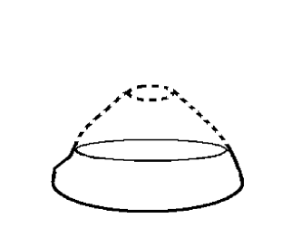
Figure 2: A cartoon of the exterior geometry cut off by a larger ‘floating’ brane.

5.1 Floating Branes

To this end, consider the bulk fields sourced by a codimension-2 brane, which we imagine is regularized by a codimension-1 brane situated at $r=r_{b}$, as before. Now, imagine drawing a large, fictitious circle at a much larger radius $\bar{r}\gg r_{b}$, but which is nevertheless much smaller than the typical scale (such as $l_{\scriptscriptstyle W}$) defined by the bulk geometry. We place a fictitious codimension-1 ‘floating’ brane (and, by dimensional reduction, an implicit effective codimension-2 brane) at $\bar{r}$, and replace the full geometry for $r<\bar{r}$ by a nonsingular cap geometry. As before, we ask this interior geometry to match continuously to the exterior solution at $r=\bar{r}$, but with the important difference that this time we use these conditions to fix integration constants in the interior solution, with the exterior geometry regarded as given (rather than the other way around, as before).

When $V$ is negligible near the brane we use precisely the same exterior solution as before, eqs. (25) and (26), and so find the following values at $r=\bar{r}$:

$$e^{\bar{\phi}}=e^{\phi_{b}}\left(\frac{\bar{r}-l}{r_{b}-l}\right)^{p_{\phi}},\qquad e^{\bar{B}}=r_{b}\left(\frac{\bar{r}-l}{r_{b}-l}\right)^{p_{\scriptscriptstyle B}}\,,$$ (92)

and

$$e^{(d-1)\overline{W}}=\frac{\left[(r_{b}-l)/l_{\scriptscriptstyle W}\right]^{\Omega}+\left[l_{\scriptscriptstyle W}/(r_{b}-l)\right]^{\Omega}}{\left[(\bar{r}-l)/l_{\scriptscriptstyle W}\right]^{\Omega}+\left[l_{\scriptscriptstyle W}/(\bar{r}-l)\right]^{\Omega}}\left(\frac{r_{b}-l}{\bar{r}-l}\right)^{p_{\scriptscriptstyle B}}e^{(d-1)W_{b}}\,.$$ (93)

The goal is to repeat the arguments of the previous sections to express the near-brane derivatives in terms of an action defined at $\bar{r}$ rather than $r_{b}$. This is useful because in any limit where $r_{b}$ and $l$ are taken to zero, the quantities $\bar{\phi}$, $\bar{B}$ and $\overline{W}$ will be held constant.

Continuity and regularity at the potential singularity at $r=0$ require the interior ‘floating’ solution (for negligible $V$) to become

$$\phi_{f}=\bar{\phi}\,,\quad e^{B_{f}}=\left(\frac{r}{\bar{r}}\right)^{p}e^{\bar{B}}\quad\hbox{and}\quad e^{(d-1)W_{f}}=\left[\frac{\bar{r}^{2p}+l_{{\scriptscriptstyle W}f}^{2p}}{r^{2p}+l_{{\scriptscriptstyle W}f}^{2p}}\right]\,e^{(d-1)\overline{W}}\,,$$ (94)

where $p$ is chosen to ensure the geometry has no conical defects. To determine what this requires we write the proper distance within the cap (see appendix A) as

$${\hbox{d}}\rho=e^{B_{f}+dW_{f}}\,{\hbox{d}}\ln r=e^{\bar{B}+d\overline{W}}\,\left(\frac{r}{\bar{r}}\right)^{p}\left[\frac{\bar{r}^{2p}+l_{{\scriptscriptstyle W}f}^{2p}}{r^{2p}+l_{{\scriptscriptstyle W}f}^{2p}}\right]^{d/(d-1)}\frac{{\hbox{d}}r}{r}\,,$$ (95)

where $\xi_{f}=1$ is chosen to ensure continuity of ${\hbox{d}}\rho/{\hbox{d}}r$ at $r=\bar{r}$. In terms of $\rho$ we have $e^{B_{f}}=\alpha_{f}\,\rho+{\cal O}(\rho^{3})$, with

$$\alpha_{f}=p\,e^{-d\overline{W}}\,\left[1+\left(\frac{\bar{r}}{l_{{\scriptscriptstyle W}f}}\right)^{2p}\right]^{-d/(d-1)}\,,$$ (96)

and so to avoid a conical singularity we choose

$$p=e^{d\overline{W}}\left[1+\left(\frac{\bar{r}^{2}}{l_{{\scriptscriptstyle W}f}}\right)^{2p}\right]^{d/(d-1)}>0\,.$$ (97)

Notice that, unlike for the regularized brane, $W_{f}$ and $e^{B_{f}}$ need not vanish at the same place. As before, the constant $l_{{\scriptscriptstyle W}f}$ is set by continuity of the on-brane curvature, with

$$R=\frac{4d\,p^{2}}{(d-1)\bar{r}^{2}}\left(\frac{\bar{r}}{l_{{\scriptscriptstyle W}f}}\right)^{2p}\left[1+\left(\frac{\bar{r}}{l_{{\scriptscriptstyle W}f}}\right)^{2p}\right]^{-2}e^{-2(d-1)\overline{W}}=\frac{4d\,p^{2/d}}{(d-1)\bar{r}^{2}}\left(\frac{\bar{r}}{l_{{\scriptscriptstyle W}f}}\right)^{2p}\,.$$ (98)

Turning to the jump conditions across $r=\bar{r}$, we come to the main point: we define the brane action at $\bar{r}$ by the condition that it produce the required discontinuity in the bulk field derivatives. That is, we now regard eqs. (68) – (70) (reproduced again here)

$$\frac{\kappa^{2}{\overline{T}_{2}}^{\prime}(\overline{\phi})}{2\pi} = \left(e^{\overline{B}_{e}+d\overline{W}_{e}}\partial_{\rho}\phi_{e}\right)_{\rho=\overline{\rho}}$$ (99)

$$\frac{\kappa^{2}\overline{T}_{2}(\overline{\phi})}{2\pi} \simeq 1-\left(e^{\overline{B}_{e}+d\overline{W}_{e}}\,\Bigl{[}(d-1)\partial_{\rho}W_{e}+\partial_{\rho}B_{e}\Bigr{]}\right)_{\rho=\overline{\rho}}$$ (100)

$$\frac{\kappa^{2}\overline{U}_{2}(\overline{\phi})}{2\pi} \simeq \left(d\,e^{\overline{B}_{e}+d\overline{W}_{e}}\partial_{\rho}W_{e}\right)_{\rho=\overline{\rho}}$$ (101)

as being solved for the effective actions, $\overline{T}_{2}$ and $\overline{U}_{2}$, given the known external bulk profiles sourced by the underlying regularized brane defined at $r=r_{b}$ (together with the singularity-free internal profiles they match across to at $r=\overline{r}$). The approximate equalities in these equations indicate the neglect of $\bar{r}^{2}R\propto(\bar{r}/l_{{\scriptscriptstyle W}f})^{2p}$, as was also done in earlier sections when neglecting $r_{b}^{2}R$ in eqs. (68) to (70).

One might worry that the three conditions, eqs. (99) through (101), might overdetermine the two functions $\overline{T}_{2}$ and $\overline{U}_{2}$, however this does not happen ultimately because these equations are related to one another by the bulk field equations and Bianchi identities. In fact, since any solution is required to satisfy the curvature constraint — c.f. eq. (78),

$$\overline{\cal U}_{2}\left\{2-2\,\overline{\cal T}_{2}-\left(\frac{d-1}{d}\right)\overline{\cal U}_{2}\right\}-\left({\overline{\cal T}_{2}}^{\prime}\right)^{2}\simeq 0\,,$$ (102)

this provides the most efficient means for finding $\overline{U}_{2}$ given $\overline{T}_{2}$, and vice versa, where $\overline{\cal T}_{2}=\kappa^{2}\overline{T}_{2}/2\pi$ and $\overline{\cal U}_{2}=\kappa^{2}\overline{U}_{2}/2\pi$.

Renormalized actions and near-brane asymptotics

Once the renormalized action is constructed in this way, it can be related to the integration constants of the bulk solutions. For instance, if we assume solutions are given by eqs. (92) and (93), then the constants $\xi$, $p_{\phi}$ and $p_{\scriptscriptstyle B}$ are directly related to the renormalized action by

$$\xi p_{\phi}=\frac{\kappa^{2}\overline{T}_{2}^{\prime}}{2\pi}\quad\hbox{and}\quad\xi p_{\scriptscriptstyle B}=1-\frac{\kappa^{2}}{2\pi}\left[\overline{T}_{2}+\left(\frac{d-1}{d}\right)\overline{U}_{2}\right]\,.$$ (103)

The main difference between these and earlier formulae comes from the observation that their right-hand sides remain finite as $r_{b},l\to 0$ with $\bar{r}$ and $\xi=[1-(l/r_{b})]^{-1}$ fixed. We may accordingly use in them $l_{\scriptscriptstyle W}\gg\bar{r}\gg|l|$, while we earlier had $l_{\scriptscriptstyle W}\gg r_{b}\simeq|l|$.

5.2 Codimension-2 RG Flow

Rather than directly solving the above equations, it is often simpler instead to obtain the renormalized action by solving an appropriate renormalization group (RG) equation. In this section we derive such an equation for the floating brane action, using the bulk field equations and brane junction conditions. We then examine in detail their form for a special case already studied in the literature [19] using perturbative methods, reproducing the previous results and extending them taking into account the coupling with gravity.

Derivation of the RG equations

Since the position of the floating brane, $\overline{r}$, is completely arbitrary, physical quantities do not depend on it. This is true in particular for the bulk field profiles themselves, since the floating brane tension, $\overline{T}_{2}$, and on-brane potential, $\overline{U}_{2}$, are defined to vary with $\bar{r}$ in precisely the way required to leave bulk field profiles unchanged. This observation provides an alternative way to derive these renormalized quantities: by setting up and solving the differential conditions that express the independence of the bulk fields to changes in $\bar{r}$. The resulting equations are RG equations inasmuch as they express the independence of quantities under changes to $\bar{r}$, in much the same way as more traditional RG equations express the independence of physical quantities to the arbitrary renormalization point, $\mu$.

Since the relationship between the brane action and the bulk fields is dictated by the field equations themselves, we derive the floating equations by using the junction conditions after directly applying the differential operator

$${\cal D}=e^{\overline{B}+d\overline{W}}\frac{\partial}{\partial\overline{\rho}}\,,$$ (104)

to the renormalized actions, where it is understood that all the integration constants in the external bulk fields are held fixed when doing so. This means that ${\cal D}$ agrees with $e^{B_{e}+dW_{e}}\partial_{\rho}=\xi(r-l)\partial_{r}$ when applied to external bulk fields, with $r$ then taken to $\bar{r}$. The same need not be true for the interior solutions, since — c.f. eqs. (94) — these have integration constants that depend explicitly on $\bar{r}$ (and so on $\bar{\rho}$). To derive the RG equation we therefore apply ${\cal D}$ to the junction conditions, eqs. (65) through (67), and simplify the result using the bulk field equations.

For example, applying ${\cal D}$ to eq. (65) gives

$${\cal D}\;\frac{\kappa^{2}{\overline{T}_{2}}^{\prime}}{2\pi} = \left(e^{B_{e}+dW_{e}}\partial_{\rho}\Bigl{[}e^{B_{e}+dW_{e}}\partial_{\rho}\phi_{e}\Bigr{]}\right)_{\rho=\overline{\rho}}-\left(e^{\bar{B}+d\overline{W}}\partial_{\bar{\rho}}\Bigl{[}e^{B_{f}+dW_{f}}\partial_{\rho}\phi_{f}\Bigr{]}_{\rho=\overline{\rho}}\right)$$ (105)

$$= \Bigl{[}e^{B+dW}\partial_{\rho}\Bigl{(}e^{B+dW}\partial_{\rho}\phi\Bigr{)}\Bigr{]}_{b}-\left(e^{\bar{B}+d\overline{W}}\partial_{\bar{\rho}}\alpha^{a}\right)\left[\frac{\partial}{\partial\alpha^{a}}\left(e^{B_{f}+dW_{f}}\partial_{\rho}\phi_{f}\right)\right]_{\rho=\bar{\rho}}$$

$$= -\left(e^{B_{f}+dW_{f}}\partial_{\bar{\rho}}\alpha^{a}\right)\left[\frac{\partial}{\partial\alpha^{a}}\left(e^{B_{f}+dW_{f}}\partial_{\rho}\phi_{f}\right)\right]_{\rho=\bar{\rho}}\,,$$

where, as before, $\Bigl{[}X\Bigr{]}_{b}$ denotes the jump of the quantity $X$ across $\rho=\bar{\rho}$, and the $\alpha^{a}$ collectively denote the integration constants of the interior solution. The last equality then uses the dilaton field equation, eq. (2.1), to write the discontinuity as $\Bigl{[}e^{2(B+dW)}\kappa^{2}V^{\prime}\Bigr{]}_{b}$, which vanishes because of the continuity of $\phi$ and $V$ across the brane. When $V$ is negligible in the near-brane limit, the right-hand-side of the last equality in eq. (105) can be evaluated explicitly using the known cap solutions, giving

$${\cal D}\;\frac{\kappa^{2}{\overline{T}_{2}}^{\prime}}{2\pi}=0\,,$$ (106)

because $\partial_{\rho}\phi_{f}=0$.

Similarly, applying ${\cal D}$ to eq. (67) and using the $(\mu\nu)$ Einstein equation of eq. (2.1) gives

$${\cal D}\;\frac{\kappa^{2}{\overline{U}_{2}}}{2\pi} = \Bigl{[}e^{B+dW}\partial_{\rho}\Bigl{(}e^{B+dW}\partial_{\rho}W\Bigr{)}\Bigr{]}_{b}-\left(e^{\bar{B}+d\overline{W}}\partial_{\bar{\rho}}\alpha^{a}\right)\left[\frac{\partial}{\partial\alpha^{a}}\left(e^{B_{f}+dW_{f}}\partial_{\rho}W_{f}\right)\right]_{\rho=\bar{\rho}}$$ (107)

$$= -\left(e^{\bar{B}+d\overline{W}}\partial_{\bar{\rho}}\alpha^{a}\right)\left[\frac{\partial}{\partial\alpha^{a}}\left(e^{B_{f}+dW_{f}}\partial_{\rho}W_{f}\right)\right]_{\rho=\bar{\rho}}\,,$$

which uses the continuity of $e^{2(B+dW)}[\check{R}+2\kappa^{2}V]$ across $r=\bar{r}$. Finally, applying ${\cal D}$ to eq. (66) and using the $(\mu\nu)$ and $(\theta\theta)$ equations of (2.1) implies

$${\cal D}\;\frac{\kappa^{2}{\overline{T}_{2}}}{2\pi}=\left(e^{\bar{B}+d\overline{W}}\partial_{\bar{\rho}}\alpha^{a}\right)\left[\frac{\partial}{\partial\alpha^{a}}\left(e^{B_{f}+dW_{f}}\partial_{\rho}\Bigl{[}(d-1)W_{f}+B_{f}\Bigr{]}\right)\right]_{\rho=\overline{\rho}}\,,$$ (108)

which uses continuity of $e^{2(B+dW_{e})}\left[\left({(d-1)}/{d}\right)\check{R}+2\kappa^{2}V\right]$.

When $V$ is negligible near the brane (and so also inside the cap) we can evaluate the relevant derivatives explicitly, using $e^{B_{f}+dW_{f}}\partial_{\rho}X_{f}=r\partial_{r}X_{f}$ with

$$r\partial_{r}B_{f}=p\quad\hbox{and}\quad r\partial_{r}W_{f}=-\frac{2p}{d-1}\left(\frac{r^{2p}}{r^{2p}+l_{{\scriptscriptstyle W}f}^{2p}}\right)\,,$$ (109)

and so

$$\left(e^{\bar{B}+d\overline{W}}\partial_{\bar{\rho}}\alpha^{a}\right)\left[\frac{\partial}{\partial\alpha^{a}}\left(e^{B_{f}+dW_{f}}\partial_{\rho}B_{f}\Bigr{]}\right)\right]_{\rho=\overline{\rho}}=\bar{r}\partial_{\bar{r}}p\,,$$ (110)

and

$$\left(e^{\bar{B}+d\overline{W}}\partial_{\bar{\rho}}\alpha^{a}\right)\left[\frac{\partial}{\partial\alpha^{a}}\left(e^{B_{f}+dW_{f}}\partial_{\rho}W_{f}\Bigr{]}\right)\right]_{\rho=\overline{\rho}}$$ (111)

$$\qquad\qquad\qquad\qquad=\left\{\left[\bar{r}\partial_{\bar{r}}p\left(\frac{\partial}{\partial p}\right)+\bar{r}\partial_{\bar{r}}l_{{\scriptscriptstyle W}f}\left(\frac{\partial}{\partial l_{{\scriptscriptstyle W}f}}\right)\right]\left[-\frac{2p}{d-1}\left(\frac{r^{2p}}{r^{2p}+l_{{\scriptscriptstyle W}f}^{2p}}\right)\right]\right\}_{r=\bar{r}}\,.$$

Rather than using these expressions, however, it is much more convenient to use (106) to determine $\overline{T}_{2}$, and then directly use the constraint, eq. (102), to find $\overline{U}_{2}$. We now illustrate how this works in more detail by considering a simple example.

An example

To better understand the RG equation’s implications, we follow [19] and expand the $\phi$-dependence of the codimension-2 tension in a complete basis,

$${\cal T}_{2}(\phi)=\sum_{n=0}^{\infty}\,\lambda_{2n}\,\frac{\phi^{2n}}{(2n)!}\,,$$ (112)

where the constants $\lambda_{2n}$ are effective coupling constants that control the coupling of the bulk scalar to the brane, that are $\phi$-independent by definition. Since $\phi=\phi(\bar{r})$ depends explicitly on $\bar{r}$ (through the bulk scalar profile) while ${\cal T}_{2}^{\prime}$ does not, the renormalized couplings $\lambda_{2n}$ must depend implicitly on $\bar{r}$. Our goal is to use the RG equations to extract this dependence explicitly.

To this end we insert the form (112) in equation (106), obtaining

$$0={\cal D}{\cal T}_{2}^{\prime} = \sum_{n=1}^{\infty}\left[{\cal D}\lambda_{2n}\,\frac{\phi^{2n-1}}{(2n-1)!}+\lambda_{2n}\frac{\phi^{2n-2}}{(2n-2)!}\,{\cal D}\phi\right]$$ (113)

$$= \sum_{n=1}^{\infty}\left[{\cal D}\lambda_{2n}\,\frac{\phi^{2n-1}}{(2n-1)!}+\lambda_{2n}\frac{\phi^{2n-2}}{(2n-2)!}\left(\sum_{p=1}^{\infty}\,\lambda_{2p}\frac{\phi^{2p-1}}{(2p-1)!}\right)\right]$$

$$= \sum_{n=1}^{\infty}\,c_{2n}\,\frac{\phi^{2n-1}}{(2n-1)!}$$

where to pass from the first to the second line we use the dilaton junction condition (99), ${\cal D}\phi={{\cal T}_{2}}^{\prime}$, and the last line re-orders the sums to define

$$c_{2n}\equiv{\cal D}\lambda_{2n}+\sum_{k=1}^{n}\,\left({\begin{array}[]{*{20}c}2n-1\\ 2k-1\\ \end{array}}\right)\,\lambda_{2k}\,\lambda_{2n-2k+2}\,.$$ (114)

Crucially, the condition ${\cal D}{{\cal T}_{2}}^{\prime}=0$ applies as an identity for all values of the integration constants characterizing the bulk fields — like $\phi_{b}$, $\xi$, $R$ etc. — provided these are held fixed when $\bar{r}$ is varied. In particular, although the couplings $\lambda_{2n}$ can also depend on some of these parameters, they contain enough freedom to vary $\phi$ with the $\lambda_{2n}$’s held fixed. This implies that eq. (113) holds as an identity for all $\phi$, and so all the quantities $c_{2n}$ must separately vanish. In this way, we obtain the following renormalization group equations for the couplings $\lambda_{2n}$, for $n\geq 1$,

$${\cal D}\lambda_{2n}=\xi\hat{r}\,\frac{\partial\lambda_{2n}}{\partial\hat{r}}=-\sum_{k=1}^{n}\,\left({\begin{array}[]{*{20}c}2n-1\\ 2k-1\\ \end{array}}\right)\,\lambda_{2k}\,\lambda_{2n-2k+2}\,,$$ (115)

where $\hat{r}=\bar{r}-l$. Restricting to flat geometries having conical singularities, and keeping in mind that $\xi=\alpha$ for such geometries, these RG equations become those obtained in [19] by means of graphical methods. Our formalism, then, easily captures the RG evolution of the brane couplings, without the need of going through the perturbative calculations used in the previous literature.

Similar steps can be used to derive RG equations for the analogous couplings in ${\cal U}_{2}$,

$${\cal U}_{2}(\phi)=\sum_{n=0}^{\infty}\,\gamma_{2n}\,\frac{\phi^{2n}}{(2n)!}\,,$$ (116)

but a simpler procedure to find the $\gamma_{2n}$’s is to directly use the curvature constraint to relate them to the $\lambda_{2n}$’s. Working to leading order in $\kappa^{2}$ implies ${\cal U}_{2}\simeq\frac{1}{2}\left({{\cal T}_{2}}^{\prime}\right)^{2}$ and so

$$\gamma_{2n}\simeq\frac{1}{2}\sum_{k=1}^{n}\left({\begin{array}[]{*{20}c}2n\\ 2k-1\\ \end{array}}\right)\lambda_{2k}\lambda_{2n-2k+2}\,.$$ (117)

Notice that none of these expressions provide the renormalization group equation for the coupling $\lambda_{0}$. To obtain this we turn to the third RG equation, (108). Direct application of ${\cal D}$ to eq. (112) implies

$${\cal D}\,{\cal T}_{2}={\cal D}\lambda_{0}+\sum_{n=1}^{\infty}\,\left[{\cal D}\lambda_{2n}+\sum_{k=1}^{n}\,\left({\begin{array}[]{*{20}c}2n\\ 2k-1\\ \end{array}}\right)\,\lambda_{2k}\,\lambda_{2n-2k+2}\right]\,\frac{\phi^{2n}}{(2n)!}\,.$$ (118)

Evaluating ${\cal D}\lambda_{2n}$ with eq. (115), and using the identity

$$\left({\begin{array}[]{*{20}c}2n\\ 2k-1\\ \end{array}}\right)=\left({\begin{array}[]{*{20}c}2n-1\\ 2k-1\\ \end{array}}\right)+\left({\begin{array}[]{*{20}c}2n-1\\ 2k-2\\ \end{array}}\right)\,,$$ (119)

we find

$$0={\cal D}\lambda_{0}+\sum_{n=1}^{\infty}\,\sum_{k=1}^{n}\,\left({\begin{array}[]{*{20}c}2n-1\\ 2k-2\\ \end{array}}\right)\,\lambda_{2k}\,\lambda_{2n-2k+2}\,\left[\frac{\phi^{2n}}{(2n)!}\right]\,.$$ (120)

This expression simplifies with the following manipulations:

$$\sum_{n=1}^{\infty}\,\sum_{k=1}^{n}\,\left({\begin{array}[]{*{20}c}2n-1\\ 2k-2\\ \end{array}}\right)\,\lambda_{2k}\,\lambda_{2n-2k+2}\,\left[\frac{\phi^{2n}}{(2n)!}\right] = \frac{1}{2}\,\left(\sum_{n=1}^{\infty}\lambda_{2n}\,\frac{\phi^{2n-1}}{(2n-1)!}\right)^{2}$$ (123)

$$= \frac{1}{2}\left({{\cal T}_{2}}^{\prime}\right)^{2}=\frac{{\xi}^{2}\,p_{\phi}^{2}}{2}\,,$$ (124)

where the last equality uses the dilaton junction condition, (99).

The evolution equation for $\lambda_{0}$ then becomes

$${\cal D}\lambda_{0}+\frac{{\xi}^{2}\,p_{\phi}^{2}}{2}=\left\{\left(\bar{r}\partial_{\bar{r}}p\,\frac{\partial}{\partial p}+\bar{r}\partial_{\bar{r}}l_{{\scriptscriptstyle W}f}\,\frac{\partial}{\partial l_{{\scriptscriptstyle W}f}}\right)\left[p\left(\frac{l_{{\scriptscriptstyle W}f}^{2p}-r^{2p}}{l_{{\scriptscriptstyle W}f}^{2p}+r^{2p}}\right)\right]\right\}_{r=\bar{r}}\simeq\bar{r}\partial_{\bar{r}}p\,,$$ (125)

where the approximate equality neglects $\bar{r}^{2}R\propto(\bar{r}/l_{{\scriptscriptstyle W}f})^{2p}$ (c.f. eq. (98)). Using $r_{b}/l=\xi/(\xi-1)$ we find that neglect of $\bar{r}^{2}R$ allows eqs. (93) and (97) to simplify to

$$p \simeq e^{d\overline{W}}=\left[\left(\xi-1\right)\,\left(\frac{\bar{r}-l}{l}\right)\right]^{d(\Omega-p_{\scriptscriptstyle B})/(d-1)}$$ (126)

$$\simeq 1+\frac{p_{\phi}^{2}}{2p_{\scriptscriptstyle B}}\ln\left[(\xi-1)\left(\frac{\bar{r}-l}{l}\right)\right]+\cdots\,,$$

which uses $d(\Omega-p_{\scriptscriptstyle B})/(d-1)\simeq p_{\phi}^{2}/(2p_{\scriptscriptstyle B})\simeq\kappa^{2}{U_{2}}/(2\pi\xi)\ll 1$ in the weak-gravity limit, using eq. (72). Notice that $p\to 1$ as $\bar{r}\to r_{b}$, and because $\Omega\geq p_{\scriptscriptstyle B}$ (with $\Omega=p_{\scriptscriptstyle B}$ only when $p_{\phi}=0$) $p$ diverges as $l\to 0$.

Writing $\bar{r}\partial_{\bar{r}}p={\cal D}p$ we see that ${\cal D}(\lambda_{0}-p)+\frac{1}{2}\,\xi^{2}p_{\phi}^{2}\simeq 0$, which admits the simple solution

$$\lambda_{0}=\lambda_{0b}-1+\left[\left(\xi-1\right)\,\left(\frac{\bar{r}-l}{l}\right)\right]^{d(\Omega-p_{\scriptscriptstyle B})/(d-1)}-\frac{\xi\,p^{2}_{\phi}}{2}\,\ln\left[(\xi-1)\left(\frac{\bar{r}-l}{l}\right)\right]\,.$$ (127)

Using the weak-gravity limit — i.e. the second line of eq. (126) and the leading approximation, $\xi p_{B}\,\simeq\,1$, to eq. (4.2) — allows this solution to be rewritten

$$\lambda_{0}\simeq\lambda_{0b}+\frac{\xi\,p^{2}_{\phi}}{2\,\xi\,p_{b}}\,\ln\left[(\xi-1)\left(\frac{\bar{r}-l}{l}\right)\right]-\frac{\xi\,p^{2}_{\phi}}{2}\,\ln\left[(\xi-1)\left(\frac{\bar{r}-l}{l}\right)\right]\simeq\lambda_{0b}\,,$$ (128)

which shows that $\lambda_{0}$ does not renormalize up to ${\cal O}(\kappa^{2})$. This holds in particular for the special case of pure tension branes, for which $p_{\phi}=0$, and so $\Omega=p_{\scriptscriptstyle B}$.

In general, we see from this section how to define a complete set of RG equations for the brane-$\phi$ couplings contained in the brane action, ${\cal T}_{2}$, and on-brane potential, ${\cal U}_{2}$, generalizing earlier discussions to more general bulk configurations.

6 Conclusions

In summary, this paper uses the example of a scalar-tensor theory in $D=d+2$ dimensions to examine the detailed connection between the properties of a $d$-dimensional, codimension-2 brane and the bulk fields which it supports. The brane in question can be fundamental (e.g. a D-brane in string theory) or a low-energy artifact (like a string defect in a gauge theory), provided the length scale associated with any brane structure is much smaller than the scales associated with the fields to which it gives rise.

Our strategy for identifying this connection is to temporarily adopt a codimension-1 crutch. That is, we first regulate the codimension-2 brane as a very small codimension-1 object. The codimension-2 action is connected by dimensional reduction to the codimension-1 one, which is in turn related to the bulk properties by standard junction conditions. Once the connection between bulk and codimension-2 properties is made we kick the crutch away, confident that its details are not important for the purposes of describing only the leading low-energy behaviour.

We find the following results

• In codimension two the bulk fields generically diverge as one approaches the brane sources, and this divergence is not restricted to a purely conical defect. Typically the appearance of curvature singularities at the brane position signals a nontrivial coupling between the brane and the bulk scalar.

• There are two quantities that characterize the properties of codimension-2 branes at low energies: the effective brane tension, ${T_{2}}(\phi)$, and the brane contribution to the effective on-brane scalar potential, ${U_{2}}(\phi)$. From the point of view of the codimension-1 regulating brane these two quantities respectively correspond to the on-brane and ‘angular’ stress-energies, $T_{\mu\nu}$ and $T_{\theta\theta}$, dimensionally reduced in the angular direction.

• The codimension-2 brane tension sources the bulk scalar field in the way one would naively expect for a $\delta$-function source, with its derivative, ${{T_{2}}}^{\prime}$, controlling the appropriately-defined near-brane radial derivative of the scalar field, $\partial_{r}\phi$. The on-brane potential, ${U_{2}}$, similarly contributes in the usual way to the low-energy dynamics of any light KK zero modes, including the curvature of the low-energy metric through the low-energy Einstein equations.

• The field equation impose a general constraint relating these quantities to the on-brane curvature, that provides the generalization of the codimension-1 brane modification to the Friedmann equation. We argue that for codimension-2 branes its proper interpretation within a low-energy framework is as a constraint that relates ${U_{2}}$ to ${T_{2}}$: $4\pi{U_{2}}\simeq\kappa^{2}\left({{T_{2}}}^{\prime}\right)^{2}$. This relation shows that any dynamics that causes $\phi$ to make ${U_{2}}$ small (and so minimize the brane’s contribution to the low energy on-brane curvature), also minimizes its coupling to the codimension-2 brane tension.

All of these results are prerequisites for the exploration of the utility of codimension-2 branes for addressing low-energy problems in particle physics and cosmology, a direction of research we hope this paper encourages.

Appendix A General Axial Solutions to the Field Equations when $V=0$

This appendix provides details of how the bulk field equations in $D$ spacetime dimensions are integrated for geometries in the case $V=0$, subject to the symmetry ansatz of axial symmetry in the transverse two dimensions spanned by $(\rho,\theta)$ and maximal symmetry in the $d=D-2$ dimensions spanned by $x^{\mu}$.

Bulk Equations

The field equations to be solved when $V=0$ are

$$\phi^{\prime\prime}+\Bigl{\{}d\,W^{\prime}+B^{\prime}\Bigr{\}}\phi^{\prime} = 0\quad\hbox{($\phi$)}$$

$$\frac{\check{R}}{d}+W^{\prime\prime}+d\,(W^{\prime})^{2}+W^{\prime}B^{\prime} = 0\quad\hbox{($\mu\nu$)}$$

$$B^{\prime\prime}+(B^{\prime})^{2}+d\,W^{\prime}B^{\prime} = 0\quad\hbox{($\theta\theta$)}$$

$$d\,\Bigl{\{}W^{\prime\prime}+(W^{\prime})^{2}\Bigr{\}}+B^{\prime\prime}+(B^{\prime})^{2}+(\phi^{\prime})^{2} = 0\quad\hbox{($\rho\rho$)}\,.$$ (129)

where we use the conventions defined in the main text. The general solution to these may be written down in closed form as follows. A first integral of the dilaton and ($\theta\theta$) Einstein equations can be done by inspection to give

$$e^{B+d\,W}\phi^{\prime}=\hat{p}_{\phi}\qquad\hbox{and}\qquad e^{B+d\,W}B^{\prime}=\hat{p}_{\scriptscriptstyle B}\,,$$ (130)

for $\hat{p}_{\phi}$ and $\hat{p}_{\scriptscriptstyle B}$ arbitrary constants. These may both be integrated a second time by conveniently redefining a new radial coordinate $r$ as

$$\frac{\mathrm{d}r}{r}:=\xi\,e^{-B-dW}\mathrm{d}\rho\,,$$ (131)

in terms of which $e^{B+dW}\partial_{\rho}=\xi\,r\,\partial_{r}$. This leads to the solutions

$$e^{\phi}=e^{\phi_{0}}\left(\frac{r}{l}\right)^{p_{\phi}}\qquad\hbox{and}\qquad e^{B}=l\left(\frac{r}{l}\right)^{p_{\scriptscriptstyle B}}\,,$$ (132)

with $p_{\phi}=\hat{p}_{\phi}/\xi$ and $p_{\scriptscriptstyle B}=\hat{p}_{\scriptscriptstyle B}/\xi$, and new integration constants $\phi_{0}$ and $l$.

Similarly the combination $(\rho\rho)-(\theta\theta)$ of Einstein equations gives

$$d\Bigl{\{}W^{\prime\prime}+(W^{\prime})^{2}-W^{\prime}B^{\prime}\Bigr{\}}+(\phi^{\prime})^{2}=0\,.$$ (133)

Multiplying this through by $e^{2(B+dW)}$, and changing variables from $\rho$ to $r$, using

$$\xi^{2}(r\,\partial_{r})^{2}W = e^{B+dW}\Bigl{(}e^{B+dW}W^{\prime}\Bigr{)}^{\prime}$$ (134)

$$= e^{2[B+dW]}W^{\prime\prime}+\xi^{2}\Bigl{[}(r\,\partial_{r}B)(r\,\partial_{r}W)+d(r\,\partial_{r}W)^{2}\Bigr{]}\,,$$

then gives

$$\ddot{W}-(d-1)(\dot{W})^{2}-2\dot{B}\dot{W}+\frac{(\dot{\phi})^{2}}{d}=0\,.$$ (135)

Here over-dots denoting differentiation with respect to $\ln r$. Using eqs. (132) for $\phi$ and $B$, leads to a differential equation involving only $W$

$$\ddot{W}-2p_{\scriptscriptstyle B}\dot{W}-(d-1)(\dot{W})^{2}+\frac{p_{\phi}^{2}}{d}=0\,.$$ (136)

This equation can be regarded as a first-order equation for $\dot{W}$, and so may be directly integrated twice, leading to the following general solution

$$(d-1)W = (d-1)W_{0}-p_{\scriptscriptstyle B}\ln\left(\frac{r}{l}\right)-\ln\cosh X$$

$$\hbox{with}\quad X = \Omega\,\ln\left(\frac{r}{l_{\scriptscriptstyle W}}\right)$$

$$\hbox{and}\quad\Omega = \sqrt{p_{\scriptscriptstyle B}^{2}+\left(\frac{d-1}{d}\right)p_{\phi}^{2}}\,,$$ (137)

where $W_{0}$ and $l_{\scriptscriptstyle W}$ are the two new integration constants. We find a total of six integration constants — $\phi_{0}$, $W_{0}$, $l$, $l_{\scriptscriptstyle W}$, $p_{\phi}$ and $p_{\scriptscriptstyle B}$ — of which one ($W_{0}$) can be changed simply by re-scaling $x^{\mu}$.

Finally, the on-brane induced curvature scalar, $R$, may be obtained using the ($\mu\nu$) Einstein equation, which states

$$\xi^{2}\ddot{W}=e^{B+dW}\Bigl{(}e^{B+dW}W^{\prime}\Bigr{)}^{\prime}=-\frac{e^{2[B+dW]}\check{R}}{d}=-\frac{e^{2[B+(d-1)W]}R}{d}\,.$$ (138)

Using the explicit form just found for the solution,

$$e^{B+(d-1)W}=\frac{l\,e^{(d-1)W_{0}}}{\cosh X}=\frac{2\,l\,e^{(d-1)W_{0}}}{(r/\ell_{\scriptscriptstyle W})^{\Omega}+(\ell_{\scriptscriptstyle W}/r)^{\Omega}}\,,$$ (139)

as well as

$$\ddot{W}=-\left(\frac{\Omega^{2}}{d-1}\right)\frac{1}{\cosh^{2}X}\,,$$ (140)

we find in this way

$$R=-d\,\xi^{2}\,\ddot{W}\,e^{-2[B+(d-1)W]}=\left[\frac{d\,\xi^{2}\,\Omega^{2}}{(d-1)\,l^{2}}\right]\,e^{-2(d-1)W_{0}}\,.$$ (141)

Given these explicit functions for $B$ and $W$, we may compute the relation between $r$ and proper distance, $\rho$, by integrating

$$\xi\,\mathrm{d}\rho = e^{B+dW}\,\frac{\mathrm{d}r}{r}$$ (142)

$$= l\,e^{dW_{0}}\left(\frac{l}{r}\right)^{p_{\scriptscriptstyle B}/(d-1)}\left[\frac{2}{(r/l_{\scriptscriptstyle W})^{\Omega}+(l_{\scriptscriptstyle W}/r)^{\Omega}}\right]^{d/(d-1)}\frac{\mathrm{d}r}{r}\,,$$

which implies $\rho\propto r^{[-p_{\scriptscriptstyle B}-d\Omega]/(d-1)}$ in the limit $r\gg l_{\scriptscriptstyle W}$ while $\rho\propto r^{[-p_{\scriptscriptstyle B}+d\Omega]/(d-1)}$ when $r\ll l_{\scriptscriptstyle W}$.

The flat limit

The special case of the flat limit, $R\to 0$, can be seen to correspond to the choice $W_{0}\to\infty$ and $l_{\scriptscriptstyle W}\to\infty$, with the ratio $e^{(d-1)W_{0}}/l_{\scriptscriptstyle W}^{\Omega}\equiv\frac{1}{2}\,e^{(d-1)w_{0}}l^{-\Omega}$ fixed, since in this case the above expressions for $\phi$ and $B$ are unchanged, while

$$e^{(d-1)W}=\frac{2e^{(d-1)W_{0}}}{(r/l_{\scriptscriptstyle W})^{\Omega}+(l_{\scriptscriptstyle W}/r)^{\Omega}}\left(\frac{l}{r}\right)^{p_{\scriptscriptstyle B}}\to e^{(d-1)w_{0}}\left(\frac{r}{l}\right)^{\Omega-p_{\scriptscriptstyle B}}\,,$$ (143)

so the resulting solution is

$$e^{\phi}=e^{\phi_{0}}\left(\frac{r}{l}\right)^{p_{\phi}}\,,\quad e^{B}=l\left(\frac{r}{l}\right)^{p_{\scriptscriptstyle B}}\quad\hbox{and}\quad e^{(d-1)W}=e^{(d-1)w_{0}}\left(\frac{r}{l}\right)^{\Omega-p_{\scriptscriptstyle B}}\,.$$ (144)

It is useful to re-express these solutions in terms of the proper distance

$$\xi\,\rho=\left[\frac{l\,(d-1)}{-p_{\scriptscriptstyle B}+d\Omega}\right]\,e^{dw_{0}}\left(\frac{r}{l}\right)^{[-p_{\scriptscriptstyle B}+d\Omega]/(d-1)}\,,$$ (145)

giving the convenient form

$$e^{\phi}=e^{\phi_{0}}\left(\frac{\rho}{\ell}\right)^{\gamma}\,,\quad e^{B}=\ell\left(\frac{\rho}{\ell}\right)^{\beta}\quad\hbox{and}\quad e^{W}=e^{w_{0}}\left(\frac{\rho}{\ell}\right)^{\omega}\,,$$ (146)

where $\ell$ is a constant in principle calculable in terms of $l$, $\xi$, $p_{\scriptscriptstyle B}$ etc., and the powers satisfy

$$d\,\omega^{2}+\beta^{2}+\gamma^{2}=d\,\omega+\beta=1\,.$$ (147)

In terms of these the derivatives appearing in the jump conditions are

$$\partial_{\rho}\phi=\frac{\gamma}{\rho}\,,\quad\partial_{\rho}B=\frac{\beta}{\rho}\quad\hbox{and}\quad\partial_{\rho}W=\frac{\omega}{\rho}\,.$$ (148)

Appendix B Derivation of the Codimension-1 Matching Conditions

Here derive the matching conditions in detail

Gauss-Codazzi Equations

Consider a $D$-dimensional geometry which in some region is foliated into a series of surfaces, $\Sigma$. The Gauss-Codazzi equations express the Riemann tensor of the full space in terms of the intrinsic and extrinsic curvatures on these surfaces. To derive these expressions, choose coordinates in the region of interest so that the surfaces are surfaces of constant coordinate, $\rho$, and for which the metric is

$$\mathrm{d}s^{2}=\mathrm{d}\rho^{2}+\hat{g}_{mn}\,\mathrm{d}x^{m}\,\mathrm{d}x^{n}\,.$$ (149)

$\rho$ clearly measures the proper distance between the surfaces. In these coordinates $\hat{g}_{mn}=\hat{g}_{mn}(\rho,x)$ defines the intrinsic geometry on the surfaces $\Sigma$. The intrinsic curvature tensor, ${{\hat{R}^{m}}}_{\;\;{nrs}}$, is defined in the usual way from the Christoffel symbols, $\hat{\Gamma}^{m}_{nr}=\frac{1}{2}\,\hat{g}^{ms}(\partial_{n}\hat{g}_{rs}+\partial_{r}\hat{g}_{ns}-\partial_{s}\hat{g}_{nr})$, by

$${{\hat{R}^{m}}}_{\;\;{nrs}}=\partial_{s}\hat{\Gamma}^{m}_{nr}+\hat{\Gamma}^{m}_{sq}\hat{\Gamma}^{q}_{nr}-(r\leftrightarrow s)\,.$$ (150)

The extrinsic curvature, $K_{mn}$, is similarly defined in terms of the unit normal, $N_{\scriptscriptstyle M}\mathrm{d}x^{\scriptscriptstyle M}={\hbox{d}}\rho$, of $\Sigma$, by

$$K_{{\scriptscriptstyle M}{\scriptscriptstyle N}}={P_{\scriptscriptstyle M}}^{\scriptscriptstyle P}{P_{\scriptscriptstyle N}}^{\scriptscriptstyle R}\nabla_{\scriptscriptstyle P}N_{\scriptscriptstyle R}$$ (151)

where ${P_{\scriptscriptstyle M}}^{\scriptscriptstyle N}=\delta_{\scriptscriptstyle M}^{\scriptscriptstyle N}-N_{\scriptscriptstyle M}N^{\scriptscriptstyle N}$ is the projector onto $\Sigma$, and so in the given coordinates we have

$$K_{mn}=\partial_{m}N_{n}-\Gamma^{\scriptscriptstyle M}_{mn}N_{\scriptscriptstyle M}=-\Gamma^{\rho}_{mn}=\frac{1}{2}\,\partial_{\rho}\hat{g}_{mn}\,,$$ (152)

which uses the following expressions for the Christoffel symbols for the full, bulk metric:

$$\Gamma^{m}_{nr}=\hat{\Gamma}^{m}_{nr}\,,\qquad\Gamma^{\rho}_{mn}=-\frac{1}{2}\,\partial_{\rho}\hat{g}_{mn}=-K_{mn}\quad\hbox{and}\quad\Gamma^{m}_{\rho n}=+\frac{1}{2}\hat{g}^{mr}\partial_{\rho}\hat{g}_{rn}={K^{m}}_{n}\,,$$ (153)

and $\Gamma^{\rho}_{\rho m}=\Gamma^{m}_{\rho\rho}=\Gamma^{\rho}_{\rho\rho}=0$.

Direct use of the definitions gives the components of the full bulk Riemann tensor as

$$R_{{mnrs}} = \hat{R}_{{mnrs}}-K_{ms}K_{nr}+K_{mr}K_{ns}$$

$$R_{{\rho mnr}} = \hat{\nabla}_{n}K_{mr}-\hat{\nabla}_{r}K_{mn}$$

$$R_{{\rho m\rho n}} = \partial_{\rho}K_{mn}-K_{ms}{K^{s}}_{n}=\nabla_{\rho}K_{mn}+K_{ms}{K^{s}}_{n}\,,$$ (154)

with any component not related to these by the symmetries of the Riemann tensor vanishing. The last line defines the quantity

$$\nabla_{\rho}K_{mn} = \partial_{\rho}K_{mn}-\Gamma^{s}_{\rho m}K_{sn}-\Gamma^{s}_{\rho n}K_{sm}$$ (155)

$$= \partial_{\rho}K_{mn}-2K_{ms}{K^{s}}_{n}\,.$$

The components of the Ricci tensor, $R_{{{\scriptscriptstyle M}{\scriptscriptstyle N}}}={{R^{{\scriptscriptstyle P}}}}_{{{\scriptscriptstyle M}{\scriptscriptstyle P}{\scriptscriptstyle N}}}$, then become

$$R_{{mn}} = \hat{R}_{{mn}}+\partial_{\rho}K_{mn}-2K_{ms}{K^{s}}_{n}+K\,K_{mn}$$

$$= \hat{R}_{{mn}}+\nabla_{\rho}K_{mn}+K\,K_{mn}$$

$$R_{{\rho m}} = \partial_{m}K-\hat{\nabla}^{n}K_{nm}$$

$$R_{{\rho\rho}} = \partial_{\rho}K+K_{mn}K^{mn}\,,$$ (156)

where $K=\hat{g}^{mn}K_{mn}={K^{m}}_{m}$. The scalar curvature is similarly given by

$$R=\hat{R}+2\,\partial_{\rho}K+K_{mn}K^{mn}+K^{2}\,.$$ (157)

Notice that

$$\partial_{\rho}\Bigl{(}\sqrt{-g}\Bigr{)}=\frac{1}{2}\sqrt{-g}\;\hat{g}^{mn}\partial_{\rho}\hat{g}_{mn}=\sqrt{-g}\;K\,,$$ (158)

which also implies the following identity

$$\partial_{\rho}\Bigl{(}\sqrt{-g}\;F\Bigr{)}=\sqrt{-g}\;\Bigl{(}\partial_{\rho}F+KF\Bigr{)}\,,$$ (159)

when $F$ is any scalar quantity. Applied to the Einstein-Hilbert action this implies

$$\sqrt{-g}\;R = \sqrt{-\hat{g}}\;\Bigl{(}\hat{R}+2\,\partial_{\rho}K+K_{mn}K^{mn}+K^{2}\Bigr{)}$$ (160)

$$= \partial_{\rho}\Bigl{(}2\,\sqrt{-g}\;K\Bigr{)}+\sqrt{-g}\;\Bigl{(}\hat{R}+K_{mn}K^{mn}-K^{2}\Bigr{)}\,.$$

Finally, the components of the full Einstein tensor, $G_{{\scriptscriptstyle M}{\scriptscriptstyle N}}=R_{{\scriptscriptstyle M}{\scriptscriptstyle N}}-\frac{1}{2}\,R\,g_{{\scriptscriptstyle M}{\scriptscriptstyle N}}$, are given by

$$G_{mn} = \hat{G}_{mn}+\nabla_{\rho}\Bigl{(}K_{mn}-K\,\hat{g}_{mn}\Bigr{)}+KK_{mn}-\frac{1}{2}\Bigl{(}K_{rs}K^{rs}+K^{2}\Bigr{)}$$

$$G_{\rho m} = \partial_{m}K-\hat{\nabla}^{n}K_{nm}$$

$$G_{\rho\rho} = \frac{1}{2}\Bigl{(}K_{mn}K^{mn}-K^{2}-\hat{R}\Bigr{)}\,.$$ (161)

Notice in particular how the second derivatives of the form $\partial_{\rho}^{2}\hat{g}_{mn}$ drop out of the expressions for $G_{\rho m}$ and $G_{\rho\rho}$, making these constraints for the purposes of integrating the equations in the $\rho$ direction from given ‘intial’ data at $\rho=\rho_{0}$.

Actions

We next turn to how these expressions are to be used to find the bulk solutions given the properties of a codimension-1 brane. This starts with the specification of a bulk and brane action, which can be specified in one of two equivalent ways. First, one can work within a bulk region, $M$, without boundaries (say), with the brane contributions explicitly inserted as delta function sources. That is, write $S=\int_{M}\mathrm{d}^{D}x\;\mathcal{L}$, with

$$\mathcal{L}=\mathcal{L}_{\scriptscriptstyle B}(\phi,A_{\scriptscriptstyle M},g_{{\scriptscriptstyle M}{\scriptscriptstyle N}})+\delta(\rho-\rho_{b})L_{b}(\phi,A_{\scriptscriptstyle M},g_{{\scriptscriptstyle M}{\scriptscriptstyle N}})\,,$$ (162)

so $S=S_{B}+S_{b}$, with $S_{B}=\int_{M}\mathrm{d}^{D}x\;\mathcal{L}_{B}$ and $S_{b}=\int_{\Sigma}\mathrm{d}^{D-1}x\;\mathcal{L}_{b}$. In this case the delta-function source in the equations of motion gives rise to step discontinuities in the $\rho$-derivatives of the bulk fields, as can be schematically inferred by integrating the field equations over a narrow region $\rho_{b}-\epsilon<\rho<\rho_{b}+\epsilon$ in a particular coordinate system (like the one used above).

Alternatively, we can divide $M$ into the two parts, $M_{\pm}$, lying on either side of $\Sigma$, with $M_{+}$ defining the region $\rho>\rho_{b}$ and $M_{-}$ denoting $\rho<\rho_{b}$. In this case we define the bulk action in the regions $M_{\pm}$ including their boundaries at $\rho=\rho_{b}$, and define the brane action only at $\rho=\rho_{b}$. In either case the goal is to identify how the brane action governs the discontinuities of the bulk fields at the brane position.

The Gibbons-Hawking Action

Because the second approach explicitly involves boundaries it is necessary to be careful about boundary contributions to actions in general, and to the gravitational action in particular. The usual gravitational action is the sum of a bulk (Einstein-Hilbert) and a boundary (Gibbons-Hawking) part, $S_{g}=S_{EH}+S_{GH}$, where

$$S_{EH}(M)=-\frac{1}{2\kappa^{2}}\int_{M}\mathrm{d}^{D}x\;\sqrt{-g}\;R\,,$$ (163)

with $\kappa^{2}=8\pi G$ related to the $D$-dimensional Newton constant.

But eq. (157) shows that this action contains terms like $\partial_{\rho}^{2}\,\hat{g}_{mn}$, and so on variation contains boundary terms of the form $\partial_{\rho}\delta\hat{g}_{mn}$. Since these derivatives can be varied independently from $\delta\hat{g}_{mn}$ on the boundary, the result is an over-constrained problem with excessively constrained boundary information. This fact does not normally cause problems when formulating solutions to Einstein’s equations without boundaries, because eq. (160) shows that these terms enter in a total derivative. When boundaries are present, the second derivative terms must be explicitly subtracted by supplementing the action by the appropriate boundary term:

$$S_{GH} = +\frac{1}{\kappa^{2}}\int_{\partial M}\mathrm{d}^{D-1}x\;\sqrt{-\hat{g}}\;K$$ (164)

$$= \frac{1}{\kappa^{2}}\int_{\Sigma(\rho_{\rm max})}\mathrm{d}^{D-1}x\;\sqrt{-\hat{g}}\;K-\frac{1}{\kappa^{2}}\int_{\Sigma(\rho_{\rm min})}\mathrm{d}^{D-1}x\;\sqrt{-\hat{g}}\;K\,.$$

With this choice the total gravitational action decomposes as follows

$$S_{g}=S_{EH}+S_{GH}=-\frac{1}{2\kappa^{2}}\int_{M}\mathrm{d}^{D}x\;\sqrt{-g}\;\Bigl{(}\hat{R}+K_{mn}K^{mn}-K^{2}\Bigr{)}\,.$$ (165)

Jump Conditions

The next step is to derive the coupling between brane and bulk in the field equations.

Israel Junction Condition

Once the surface action has been added to the gravitational kinetic term, it is possible to keep track of how its variation depends on the variation of the metric on the boundaries. Keeping track only of the boundary terms in the variation of eq. (165) leads to

$$\delta S_{g}=-\frac{1}{2\kappa^{2}}\int_{\partial M}\mathrm{d}^{D-1}x\;\sqrt{-\hat{g}}\;\Bigl{(}K^{mn}-K\hat{g}^{mn}\Bigr{)}\delta\hat{g}_{mn}+\cdots\,,$$ (166)

For a brane spanning the surface $\Sigma$ at $\rho=\rho_{b}$ lying between the two regions $M_{\pm}$ the total contribution to the equations of motion coming from variations of the boundary metric then is

$$\frac{1}{2\kappa^{2}}\Bigl{[}\sqrt{-\hat{g}}\;\Bigl{(}K^{mn}-K\hat{g}^{mn}\Bigr{)}\Bigr{]}_{\rho_{b}}+\frac{\delta S_{b}}{\delta\hat{g}_{mn}}=0\,,$$ (167)

where the notation $[F]_{\rho_{b}}$ for a bulk quantity denotes the jump

$$\Bigl{[}F\Bigr{]}_{\rho_{b}}=\lim_{\epsilon\to 0}\Bigl{[}F(\rho_{b}+\epsilon)-F(\rho_{b}-\epsilon)\Bigr{]}\,.$$ (168)

Denoting the stress energy for the bulk and brane by

$$T^{{\scriptscriptstyle M}{\scriptscriptstyle N}}=\frac{2}{\sqrt{-g}}\,\frac{\delta S_{B}}{\delta g_{{\scriptscriptstyle M}{\scriptscriptstyle N}}}\qquad\hbox{and}\qquad t^{mn}=\frac{2}{\sqrt{-\hat{g}}}\,\frac{\delta S_{b}}{\delta\hat{g}_{mn}}\,,$$ (169)

the Israel jump condition becomes

$$\Bigl{[}K_{mn}-K\hat{g}_{mn}\Bigr{]}_{\rho_{b}}+\kappa^{2}\,t_{mn}=0\,.$$ (170)

Notice that this condition could equivalently be derived in the delta-function formulation of the action, by isolating the delta-function contribution to the LHS and RHS of the $(mn)$ Einstein equation:

$$0 = \lim_{\epsilon\to 0}\int_{\rho_{b}-\epsilon}^{\rho_{b}+\epsilon}\mathrm{d}\rho\;\Bigl{\{}\Bigl{[}G_{mn}+\kappa^{2}\,T_{mn}\Bigr{]}+\delta(\rho-\rho_{b})\;\kappa^{2}\,t_{mn}\Bigr{\}}$$ (171)

$$= \Bigl{[}K_{mn}-K\,\hat{g}_{mn}\Bigr{]}_{\rho_{b}}+\kappa^{2}\,t_{mn}\,,$$

because the step discontinuity in $K_{mn}\propto\partial_{\rho}\hat{g}_{mn}$ across the brane implies a delta-function discontinuity in the contributions of $\partial_{\rho}K_{mn}$ to the Einstein tensor (see eq. (B)).

Notice also that if the brane represents a physical boundary to spacetime (rather than being a surface embedded into it), then the same arguments show that variation of the metric on the boundary leads to the boundary condition

$$\pm\frac{1}{2\kappa^{2}}\sqrt{-\hat{g}}\;\Bigl{(}K^{mn}-K\hat{g}^{mn}\Bigr{)}+\frac{\delta S_{b}}{\delta\hat{g}_{mn}}=0\,,$$ (172)

where the $+$ sign applies at the boundary at $\rho=\rho_{\rm max}$ and the $-$ sign applies at $\rho=\rho_{\rm min}$.

The Constraints

To the extent that the brane action does not support any off-brane components to stress energy, $t_{\rho m}=t_{\rho\rho}=0$, there is no discontinuity in the remaining components of the bulk Einstein equations, which then are

$$\partial_{m}K-\hat{\nabla}^{n}K_{nm}+\kappa^{2}\,T_{\rho m}=0\,,$$ (173)

expressing no net energy exchange with the brane, and

$$\frac{1}{2}\Bigl{(}K_{mn}K^{mn}-K^{2}-\hat{R}\Bigr{)}+\kappa^{2}\,T_{\rho\rho}=0\,,$$ (174)

which can be solved to give the induced curvature scalar in terms of the asymptotic forms for the bulk fields, giving

$$\hat{R}=K_{mn}K^{mn}-K^{2}-2\,\kappa^{2}\,T_{\rho\rho}\,.$$ (175)

Scalar Jump Condition

We derive the scalar jump condition in two ways: using an explicit boundary and thinking of the brane as a delta-function source.

We start with the traditional derivation. If the scalar field kinetic term has the form

$$S_{\phi}(M)=-\frac{1}{2\kappa^{2}}\int_{M}\mathrm{d}^{D}x\;\sqrt{-g}\,g^{{\scriptscriptstyle M}{\scriptscriptstyle N}}\partial_{\scriptscriptstyle M}\phi\,\partial_{\scriptscriptstyle N}\phi\,,$$ (176)

then these same arguments can be repeated to read off how the brane action gives rise to derivative discontinuities in $\phi$ at the brane positions. Since the boundary variation of eq. (176) is

$$\delta S_{\phi}=-\frac{1}{\kappa^{2}}\int_{\partial M}\mathrm{d}^{D-1}x\;\sqrt{-\hat{g}}\;N^{\scriptscriptstyle M}\partial_{\scriptscriptstyle M}\phi\,\delta\phi\,,$$ (177)

where $N_{\scriptscriptstyle M}$ is the outward-pointing normal. Combining the contributions of regions $M_{\pm}$ to that of the brane action, and keeping in mind that $N_{\scriptscriptstyle M}\mathrm{d}x^{\scriptscriptstyle M}=\mp\mathrm{d}\rho$ for the boundary between these two regions, gives

$$\frac{1}{\kappa^{2}}\Bigl{[}\sqrt{-\hat{g}}\,\partial_{\rho}\phi\Bigr{]}_{\rho_{b}}+\frac{\delta S_{b}}{\delta\phi}=0\,.$$ (178)

Alternatively, let us re-derive the jump condition by regarding the brane to be a delta-function source to the scalar field equation. Writing $S_{b}=\int\mathrm{d}^{D}x\mathcal{L}_{b}=\int\mathrm{d}^{D-1}x\,\mathrm{d}\rho\,\mathcal{L}_{b}\,\delta(\rho-\rho_{b})$, we have:

$$\sqrt{-\hat{g}}\,\Box\phi+\kappa^{2}\,\left(\frac{\partial\mathcal{L}_{b}}{\partial\phi}\right)\delta(\rho-\rho_{b})=0\,.$$ (179)

We next integrate this equation over the disk having radius $\rho=\rho_{b}+\epsilon$ and take $\epsilon\to 0^{+}$. This gives

$$\int_{0}^{\rho_{b}+\epsilon}\mathrm{d}\rho\,\partial_{\rho}\Bigl{(}\sqrt{-\hat{g}}\,\hat{g}^{\rho\rho}\partial_{\rho}\phi\Bigr{)}=\sqrt{-\hat{g}}\,\phi^{\prime}(\rho_{b}+\epsilon)=-\kappa^{2}\,\left(\frac{\partial\mathcal{L}_{b}}{\partial\phi}\right)\,.$$ (180)

In either case we have the same result:

$$\partial_{\rho}\phi(\rho\to\rho_{b}^{+})=-\frac{\kappa^{2}}{\sqrt{-\hat{g}}}\frac{\delta S_{b}}{\delta\phi}=-\frac{\kappa^{2}}{\sqrt{-\hat{g}}}\frac{\mathrm{d}}{\mathrm{d}\phi}\Bigl{(}\sqrt{-\hat{g}}\;L_{b}\Bigr{)}\,,$$ (181)

where we write $\mathcal{L}_{b}=\sqrt{-\hat{g}}\;L_{b}$. For future applications it is worth noticing that when the brane position depends on $\phi$ – i.e. $\rho_{b}=\rho_{b}(\phi)$ – the measure $\sqrt{-\hat{g}}$ does as well, and so cannot be pulled out of the derivative $\mathrm{d}/\mathrm{d}\phi$ to cancel the denominator in the prefactor.

Appendix C Matching with Derivative Corrections

For pure tension branes the junction conditions imply that the discontinuity in the combination $[W^{\prime}-B^{\prime}]$ vanishes. However this discontinuity becomes nonzero once derivative terms are included in the brane action. In this section we compute this correction.

Working to two-derivative order in the brane action we instead have

$$S_{b}=\int\mathrm{d}^{D-1}x\,\mathcal{L}_{1}=-\int\mathrm{d}^{D-1}x\sqrt{-\hat{g}}\;\left\{{T_{1}}(\phi)+\frac{1}{2}\,\hat{g}^{mn}\Bigl{(}X_{1}(\phi)\,\partial_{m}\phi\,\partial_{n}\phi+Y_{1}(\phi)\,\hat{R}_{mn}\Bigr{)}\right\}\,.$$ (182)

We imagine working with canonical kinetic terms in the bulk and so are not free to redefine the metric and scalar to remove the functions $X_{1}$ and $Y_{1}$. Given this action the brane stress energy becomes

$$t^{mn}=-\hat{g}^{mn}\,\left\{{T_{1}}+\frac{1}{2}\,\Bigl{(}X_{1}\partial_{s}\phi\,\partial^{s}\phi+Y_{1}\hat{R}\Bigr{)}+\hat{\Box}Y_{1}\right\}+X_{1}\partial^{m}\phi\,\partial^{n}\phi+Y_{1}\hat{R}^{mn}+\hat{\nabla}^{m}\hat{\nabla}^{n}Y_{1}\,.$$ (183)

Using this in the Israel junction condition

$$\Bigl{[}K_{mn}-K\,\hat{g}_{mn}\Bigr{]}+\kappa^{2}\,t_{mn}=0\,,$$ (184)

now gives

$$\Bigl{[}(D-3)W^{\prime}+B^{\prime}\Bigr{]}\check{g}_{\mu\nu} = -\check{g}_{\mu\nu}\,\kappa^{2}\left\{{T_{1}}+\frac{1}{2}\,\Bigl{(}X_{1}\partial_{s}\phi\,\partial^{s}\phi+Y_{1}\hat{R}\Bigr{)}+\hat{\Box}Y_{1}\right\}$$

$$\qquad\qquad+\kappa^{2}\Bigl{(}X_{1}\partial_{\mu}\phi\,\partial_{\nu}\phi+Y_{1}\hat{R}_{\mu\nu}+\hat{\nabla}_{\mu}\hat{\nabla}_{\nu}Y_{1}\Bigr{)}$$

$$\Bigl{[}(D-2)\,W^{\prime}\Bigr{]}g_{\theta\theta} = -g_{\theta\theta}\,\kappa^{2}\left\{{T_{1}}+\frac{1}{2}\,\Bigl{(}X_{1}\partial_{s}\phi\,\partial^{s}\phi+Y_{1}\hat{R}\Bigr{)}+\hat{\Box}Y_{1}\right\}$$ (185)

$$\qquad\qquad+\kappa^{2}\Bigl{(}X_{1}\partial_{\theta}\phi\,\partial_{\theta}\phi+Y_{1}\hat{R}_{\theta\theta}+\hat{\nabla}_{\theta}\hat{\nabla}_{\theta}Y_{1}\Bigr{)}\,,$$

or, equivalently,

$$\Bigl{(}X_{1}\partial_{\mu}\phi\,\partial_{\nu}\phi+Y_{1}\hat{R}_{\mu\nu}+\hat{\nabla}_{\mu}\hat{\nabla}_{\nu}Y_{1}\Bigr{)} = \frac{1}{D-2}\,\check{g}_{\mu\nu}\,\check{g}^{\lambda\sigma}\Bigl{(}X_{1}\partial_{\lambda}\phi\,\partial_{\sigma}\phi+Y_{1}\hat{R}_{\lambda\sigma}+\hat{\nabla}_{\lambda}\hat{\nabla}_{\sigma}Y_{1}\Bigr{)}$$

$$\Bigl{[}(D-3)W^{\prime}+B^{\prime}\Bigr{]} = -\kappa^{2}\left\{{T_{1}}+\frac{1}{2}\,\Bigl{(}X_{1}\partial_{s}\phi\,\partial^{s}\phi+Y_{1}\hat{R}\Bigr{)}+\hat{\Box}Y_{1}\right\}$$

$$\qquad\qquad+\frac{\kappa^{2}}{D-2}\,\check{g}^{\mu\nu}\Bigl{(}X_{1}\partial_{\mu}\phi\,\partial_{\nu}\phi+Y_{1}\hat{R}_{\mu\nu}+\hat{\nabla}_{\mu}\hat{\nabla}_{\nu}Y_{1}\Bigr{)}$$

$$\Bigl{[}(D-2)W^{\prime}\Bigr{]} = -\kappa^{2}\left\{{T_{1}}+\frac{1}{2}\,\Bigl{(}X_{1}\partial_{s}\phi\,\partial^{s}\phi+Y_{1}\hat{R}\Bigr{)}+\hat{\Box}Y_{1}\right\}$$

$$\qquad\qquad+\kappa^{2}g^{\theta\theta}\Bigl{(}X_{1}\partial_{\theta}\phi\,\partial_{\theta}\phi+Y_{1}\hat{R}_{\theta\theta}+\hat{\nabla}_{\theta}\hat{\nabla}_{\theta}Y_{1}\Bigr{)}\,,$$

Now the difference of the last two conditions gives

$$\Bigl{[}W^{\prime}-B^{\prime}\Bigr{]}=\kappa^{2}g^{\theta\theta}\Bigl{(}X_{1}\partial_{\theta}\phi\,\partial_{\theta}\phi+Y_{1}\hat{R}_{\theta\theta}+\hat{\nabla}_{\theta}\hat{\nabla}_{\theta}Y_{1}\Bigr{)}-\frac{\kappa^{2}}{D-2}\,\check{g}^{\mu\nu}\Bigl{(}X_{1}\partial_{\mu}\phi\,\partial_{\nu}\phi+Y_{1}\hat{R}_{\mu\nu}+\hat{\nabla}_{\mu}\hat{\nabla}_{\nu}Y_{1}\Bigr{)}\,.$$ (187)

Specializing these jump conditions to the case where all quantities are independent of $\theta$ and the $x^{\mu}$ directions are maximally symmetric then reduces them to

$$\Bigl{[}(D-3)W^{\prime}+B^{\prime}\Bigr{]} = -\kappa^{2}\left({T_{1}}+\frac{D-4}{2\,(D-2)}\;Y_{1}\check{R}\right)$$

$$\Bigl{[}(D-2)W^{\prime}\Bigr{]} = -\kappa^{2}\left({T_{1}}+\frac{1}{2}\,Y_{1}\check{R}\right)\,,$$ (188)

and so

$$\Bigl{[}W^{\prime}-B^{\prime}\Bigr{]}=-\frac{\kappa^{2}}{D-2}\,Y_{1}\check{R}\,.$$ (189)

In the general case the scalar jump condition generalizes to

$$\Bigl{[}\phi^{\prime}\Bigr{]}+\frac{\kappa^{2}}{\sqrt{-\hat{g}}}\,\frac{\delta S_{b}}{\delta\phi}=\Bigl{[}\phi^{\prime}\Bigr{]}-\frac{\kappa^{2}}{\sqrt{-\hat{g}}}\,\left\{\sqrt{-\hat{g}}\left[{T_{1}}+\frac{1}{2}\,\Bigl{(}X_{1}\partial_{s}\phi\,\partial^{s}\phi+Y_{1}\hat{R}\Bigr{)}\right]\right\}^{\prime}=0\,,$$ (190)

and for maximal symmetry in the $x^{\mu}$ directions and a symmetry under shifts in $\theta$ this simplifies to

$$\Bigl{[}\phi^{\prime}\Bigr{]}+\frac{\kappa^{2}}{\sqrt{-\hat{g}}}\,\frac{\delta S_{b}}{\delta\phi}=\Bigl{[}\phi^{\prime}\Bigr{]}-\frac{\kappa^{2}}{\sqrt{-\hat{g}}}\left\{\sqrt{-\hat{g}}\left[{T_{1}}+\frac{1}{2}\,Y_{1}\check{R}\right]\right\}^{\prime}=0\,,$$ (191)

Appendix D Explicit Solution to the jump conditions when $R=0$

We next explicitly solve the junction conditions in $D$ spacetime dimensions for the special case of the flat, $R=0$, solutions given in the main text, using only lowest-derivative terms in the brane action. We therefore take the interior solution to be the trivial one: constants $W_{i}=0$ and $\phi_{i}=\phi_{b}$, and $e^{B_{i}}=\rho$. The exterior solution by contrast is given by

$$e^{\phi_{e}}=e^{\phi_{b}}\left(\frac{\rho+\ell}{\rho_{b}+\ell}\right)^{\gamma}\,,\qquad e^{W_{e}}=\left(\frac{\rho+\ell}{\rho_{b}+\ell}\right)^{\omega}\qquad\hbox{and}\qquad e^{B_{e}}=\rho_{b}\left(\frac{\rho+\ell}{\rho_{b}+\ell}\right)^{\beta}\,,$$ (192)

where $\rho_{b}>-\ell$ and continuity of $\phi$, $W$ and $B$ from the cap geometry to the exterior bulk have been used. The bulk field equations imply the powers $\omega$, $\beta$ and $\gamma$ satisfy eq. (18): $(D-2)\omega+\beta=(D-2)\omega^{2}+\beta^{2}+\gamma^{2}=1$.

The derivative discontinuities at the brane are

$$\Bigl{[}\partial_{\rho}\phi\Bigr{]}_{b}=\frac{\gamma}{\rho_{b}+\ell}\,,\quad\Bigl{[}\partial_{\rho}W\Bigr{]}_{b}=\frac{\omega}{\rho_{b}+\ell}\quad\hbox{and}\quad\Bigl{[}\partial_{\rho}B\Bigr{]}_{b}=\frac{\beta}{\rho_{b}+\ell}-\frac{1}{\rho_{b}}=\frac{(\beta-1)\rho_{b}-\ell}{\rho_{b}(\rho_{b}+\ell)}\,,$$ (193)

so the jump conditions become

$$\Bigl{[}\phi^{\prime}\Bigr{]}_{b} = \frac{\gamma}{\rho_{b}+\ell}=\frac{\kappa^{2}}{\rho_{b}}\left\{\rho_{b}{T_{1}}(\phi_{b})+\frac{n^{2}}{2\rho_{b}}\,{Z_{1}}(\phi_{b})\right\}^{\prime}$$

$$\Bigl{[}W^{\prime}-B^{\prime}\Bigr{]}_{b} = \frac{\omega-\beta}{\rho_{b}+\ell}+\frac{1}{\rho_{b}}=\frac{(\omega-\beta+1)\rho_{b}+\ell}{\rho_{b}(\rho_{b}+\ell)}=\frac{n^{2}\kappa^{2}{Z_{1}}}{\rho_{b}^{2}}$$

$$\Bigl{[}W^{\prime}\Bigr{]}_{b} = \frac{\omega}{\rho_{b}+\ell}=-\frac{\kappa^{2}}{D-2}\,\left\{{T_{1}}-\frac{n^{2}}{2\rho_{b}^{2}}\,{Z_{1}}\right\}\,.$$ (194)

We first solve for $\omega$, $\beta$ and $\gamma$, using the $W^{\prime}$ jump condition together with eqs. (18). Defining

$$\mathcal{X}=(\rho_{b}+\ell)\kappa^{2}\left\{{T_{1}}-\frac{n^{2}}{2\rho_{b}^{2}}\,{Z_{1}}\right\}\,,$$ (195)

we find

$$\omega=-\frac{\mathcal{X}}{D-2}\,,\quad\beta=1+\mathcal{X}\quad\hbox{and}\quad\gamma^{2}=-\mathcal{X}\left(2+\frac{D-1}{D-2}\,\mathcal{X}\right)\,.$$ (196)

As before, the condition $\gamma^{2}\geq 0$ implies

$$-\frac{D-2}{D-1}\leq\frac{\mathcal{X}}{2}\leq 0\,,$$ (197)

and so the condition $\rho_{b}>-\ell$ only allows solutions in the right range to exist if ${T_{1}}<n^{2}{Z_{1}}/(2\rho_{b}^{2})$. This range for $\mathcal{X}$ also implies

$$0\leq\omega\leq\frac{2}{D-1}\,,\quad-\frac{D-3}{D-1}\leq\beta\leq 1\quad\hbox{and}\quad 0\leq\gamma^{2}\leq\frac{D-2}{D-1}\,.$$ (198)

To eliminate $\ell$ use the $\phi^{\prime}$ junction condition, $\gamma/(\rho_{b}+\ell)=(\kappa^{2}/\rho_{b})\Bigl{\{}\rho_{b}{T_{1}}+n^{2}{Z_{1}}^{\prime}/(2\rho_{b})\Bigr{\}}^{\prime}$, to write

$$\mathcal{X}=(\rho_{b}+\ell)\kappa^{2}\left\{{T_{1}}-\frac{n^{2}}{2\rho_{b}^{2}}\,{Z_{1}}\right\}=\frac{\gamma[\rho_{b}{T_{1}}-n^{2}{Z_{1}}/(2\rho_{b})]}{[\rho_{b}{T_{1}}+n^{2}{Z_{1}}/(2\rho_{b})]^{\prime}}=\frac{\gamma({\cal T}-{\cal Z})}{{\cal T}^{\prime}+{\cal Z}^{\prime}}\,,$$ (199)

where the dimensionless quantities ${\cal T}=\rho_{b}\kappa^{2}{T_{1}}$ and ${\cal Z}={n^{2}\kappa^{2}{Z_{1}}}/({2\rho_{b}})$ are as defined in the main text. Using eq. (199) in the solution, eq. (196), allows $\gamma$ to be solved completely in terms of $\rho_{b}$, ${T_{1}}$ and its derivatives. This leads to the expressions

$$\omega=\frac{2\,\chi^{2}}{(D-2)+(D-1)\chi^{2}}\,,\quad\beta=\frac{(D-2)-(D-3)\chi^{2}}{(D-2)+(D-1)\chi^{2}}\quad\hbox{and}\quad\gamma=-\frac{2(D-2)\chi}{(D-2)+(D-1)\chi^{2}}\,,$$ (200)

where now

$$\frac{1}{\chi}=\frac{[\rho_{b}{T_{1}}+n^{2}{Z_{1}}/(2\rho_{b})]^{\prime}}{\rho_{b}{T_{1}}-n^{2}{Z_{1}}/(2\rho_{b})}=\frac{{\cal T}^{\prime}+{\cal Z}^{\prime}}{{\cal T}-{\cal Z}}\,.$$ (201)

Notice that these satisfy the inequalities, eqs. (198), for all $\chi$, with the additional information that the signs of $\gamma$ and $\chi$ are opposite.

We solve for the ratio $\ell/\rho_{b}$ using the $[W^{\prime}-B^{\prime}]$ junction condition, in the form

$$\omega-\beta+1+\frac{\ell}{\rho_{b}}=+\frac{(\rho_{b}+\ell)n^{2}\kappa^{2}{Z_{1}}}{\rho_{b}^{2}}=\left(1+\frac{\ell}{\rho_{b}}\right)2\,{\cal Z}\,,$$ (202)

and find

$$\frac{\ell}{\rho_{b}}=\frac{2\,{\cal Z}-(D-1)\omega}{1-2\,{\cal Z}}=\frac{1}{1-2\,{\cal Z}}\left\{2\,{\cal Z}-\frac{2(D-1)\,\chi^{2}}{(D-2)+(D-1)\chi^{2}}\right\}\,.$$ (203)

Notice that $\rho_{b}>-\ell$ implies $\ell/\rho_{b}>-1$. Alternatively, we may solve for $\rho_{b}$ by instead using the expression for $\omega$ as a function of $\mathcal{X}$, to get

$$(D-1)\omega=-\frac{D-1}{D-2}\,\mathcal{X}=-\frac{D-1}{D-2}\left(\frac{\ell}{\rho_{b}}+1\right)\kappa^{2}\left\{\rho_{b}{T_{1}}-\frac{n^{2}{Z_{1}}}{2\rho_{b}}\right\}=\frac{D-1}{D-2}\left(\frac{\ell}{\rho_{b}}+1\right)\Bigl{(}{\cal Z}-{\cal T}\Bigr{)}\,,$$ (204)

so

$$\frac{\ell}{\rho_{b}}+1=\frac{(D-2)\omega}{{\cal Z}-{\cal T}}\,.$$ (205)

Eliminating $\ell$, by combining eqs. (203) and (205), gives an expression involving only $\omega$, ${\cal T}$ and ${\cal Z}$ (or, equivalently, only $\chi$, ${\cal T}$ and ${\cal Z}$):

$$\frac{(D-1)\,\omega-1}{1-2\,{\cal Z}}=\frac{(D-2)\omega}{{\cal T}-{\cal Z}}\,.$$ (206)

To get the final relation relating $\rho_{b}$ to $\phi_{b}$, eliminate $\omega$ in terms of $\chi$ and use eq. (201) to remove $\chi$, as in

$$\frac{1}{\omega} = \frac{(D-1)\,{\cal T}+(D-3){\cal Z}-(D-2)}{{\cal T}-{\cal Z}}$$ (207)

$$= \frac{D-1}{2}+\left(\frac{D-2}{2}\right)\frac{1}{\chi^{2}}=\frac{D-2}{2}+\frac{D-2}{2}\left[\frac{({\cal T}^{\prime}+{\cal Z}^{\prime})}{{\cal T}-{\cal Z}}\right]^{2}\,,$$

where the first line follows from eq. (206) and the second line uses eqs. (200) and (201). This can be rewritten somewhat to give the constraint

$$(D-2)({\cal T}^{\prime}+{\cal Z}^{\prime})^{2}+(D-1)({\cal T}-{\cal Z})^{2}+2({\cal T}-{\cal Z})\Bigl{[}(D-2)-(D-1)\,{\cal T}-(D-3){\cal Z}\Bigr{]}=0\,.$$ (208)

Notice that this agrees with the appropriate specialization of eq. (4.2): to $R=W_{b}=V=0$.

Conical bulk solution

The special case where the external geometry is a cone corresponds to the choices $\omega=\gamma=0$ and $\beta=1$. As the $W^{\prime}$ junction condition shows, this is only possible (given a flat cap geometry) if $t_{\theta\theta}=0$, and so

$$\rho_{b}{T_{1}}=\frac{n^{2}{Z_{1}}}{2\rho_{b}}\quad\hbox{or}\quad{\cal T}={\cal Z}\,.$$ (209)

Used in the above formulae this implies $\chi=0$, which ensures the vanishing of both $\omega$ and $\gamma$, as claimed. Eq. (209), implies $\rho_{b}$ is given by

$$\rho_{b}^{2}=\frac{n^{2}{Z_{1}}}{2{T_{1}}}\,,$$ (210)

which when used in the definition of ${\cal T}$ implies

$${\cal T}=\kappa^{2}\rho_{b}{T_{1}}=\kappa^{2}\sqrt{\frac{n^{2}{T_{1}}{Z_{1}}}{2}}\,.$$ (211)

Consequently,

$$\frac{\ell}{\rho_{b}}=\frac{2\,{\cal Z}}{1-2\,{\cal Z}}\,.$$ (212)

Finally, the condition that $\phi^{\prime}$ must vanish at the brane (recall $\gamma=0$) requires ${\cal T}+{\cal Z}=2{\cal T}$ to be $\phi$-independent, but this is only consistent with eq. (211) if the product ${T_{1}}{Z_{1}}$ is independent of $\phi$.

If, for example, we take ${T_{1}}(\phi)=U_{0}\,e^{u\phi}$ and ${Z_{1}}(\phi)=V_{0}\,e^{v\phi}$, then we may specialize the above conical-limit equations to

$$\rho_{b}=\sqrt{\frac{n^{2}V_{0}}{2U_{0}}}\;e^{(v-u)\phi_{b}/2}\quad\hbox{and}\quad{\cal T}={\cal Z}=\kappa^{2}\rho_{b}{T_{1}}=\kappa^{2}\sqrt{\frac{n^{2}U_{0}V_{0}}{2}}\;e^{(v+u)\phi_{b}/2}\,,$$ (213)

which show that ${\cal T}$ is only $\phi$-independent if $u=-v$. Notice that this includes in particular the case $u=-v=2/(D-2)$ which encodes scale invariance in the bulk field equations. Notice also that the choice $u=-v$ also implies $\rho_{b}\propto e^{v\phi_{b}}$, and so is $\phi_{b}$-dependent unless $u=v=0$.

References

- [1] L. Randall, R. Sundrum, Phys. Rev. Lett. 83 (1999) 3370 [hep-ph/9905221], Phys. Rev. Lett. 83 (1999) 4690 [hep-th/9906064].
- [2] For some preliminary examples of how codimension-2 backreaction can differ from codimension-1 see: E. Dudas, C. Papineau and V. A. Rubakov, JHEP 0603 (2006) 085 [arXiv:hep-th/0512276]; E. Dudas and C. Papineau, JHEP 0611 (2006) 010 [arXiv:hep-th/0608054]; C. P. Burgess, C. de Rham and L. van Nierop, JHEP 0808, 061 (2008) [arXiv:0802.4221 [hep-ph]].
-
[3]
G. W. Gibbons, R. Guven and C. N. Pope,
Phys. Lett. B 595 (2004) 498
[hep-th/0307238];
Y. Aghababaie et al.,
JHEP 0309 (2003) 037
[hep-th/0308064];
P. Bostock, R. Gregory, I. Navarro and J. Santiago,
Phys. Rev. Lett. 92 (2004) 221601
[hep-th/0311074];
C. P. Burgess, F. Quevedo, G. Tasinato and I. Zavala,
JHEP 0411 (2004) 069
[hep-th/0408109];
J. Vinet and J. M. Cline,
Phys. Rev. D 71 (2005) 064011
[hep-th/0501098].
- [4] J. M. Cline, J. Descheneau, M. Giovannini and J. Vinet, JHEP 0306 (2003) 048 [arXiv:hep-th/0304147]; E. Papantonopoulos, A. Papazoglou and V. Zamarias, Nucl. Phys. B 797 (2008) 520 [arXiv:0707.1396 [hep-th]]; T. Kobayashi and M. Minamitsuji, JCAP 0707 (2007) 016 [arXiv:0705.3500 [hep-th]]; F. Chen, J. M. Cline and S. Kanno, Phys. Rev. D 77 (2008) 063531 [arXiv:0801.0226 [hep-th]].
- [5] L. J. Hall, Y. Nomura and D. R. Smith, Nucl. Phys. B 639 (2002) 307 [hep-ph/0107331]; I. Gogoladze, Y. Mimura and S. Nandi, Phys. Lett. B 562 (2003) 307 [hep-ph/0302176]; C. A. Scrucca, M. Serone, L. Silvestrini and A. Wulzer, JHEP 0402 (2004) 049 [hep-th/0312267]; C. Biggio and M. Quiros, Nucl. Phys. B 703 (2004) 199 [hep-ph/0407348]; Y. Hosotani, S. Noda and K. Takenaga, Phys. Lett. B 607 (2005) 276 [hep-ph/0410193]; D. Hernandez, S. Rigolin and M. Salvatori, [arXiv:0712:1980].
- [6] S. M. Carroll and M. M. Guica, [hep-th/0302067];
- [7] Y. Aghababaie, C. P. Burgess, S. L. Parameswaran and F. Quevedo, Nucl. Phys. B 680 (2004) 389 [hep-th/0304256].
- [8] I. Navarro, Class. Quant. Grav. 20 (2003) 3603 [arXiv:hep-th/0305014]; H. P. Nilles, A. Papazoglou and G. Tasinato, Nucl. Phys. B 677 (2004) 405 [arXiv:hep-th/0309042]; H. M. Lee, Phys. Lett. B 587 (2004) 117 [arXiv:hep-th/0309050].
- [9] C. P. Burgess and D. Hoover, Nucl. Phys. B 772 (2007) 175 [arXiv:hep-th/0504004]; C. P. Burgess, J. Matias and F. Quevedo, Nucl. Phys. B 706 (2005) 71 [arXiv:hep-ph/0404135]; C. P. Burgess, Annals Phys. 313 (2004) 283 [arXiv:hep-th/0402200]; AIP Conf. Proc. 743 (2005) 417 [arXiv:hep-th/0411140]; arXiv:0708.0911 [hep-ph].
- [10] J. Vinet and J. M. Cline, Phys. Rev. D 70 (2004) 083514 [hep-th/0406141]; Phys. Rev. D 71 (2005) 064011 [arXiv:hep-th/0501098]; J. Garriga and M. Porrati, JHEP 0408 (2004) 028 [arXiv:hep-th/0406158].
- [11] K. Lanczos, Phys. Z. 23 (1922) 239–543; Ann. Phys. 74 (1924) 518–540; C.W. Misner and D.H. Sharp, Phys. Rev. 136 (1964) 571–576; W. Israel, Nuov. Cim. 44B (1966) 1–14; errata Nuov. Cim. 48B 463.
- [12] S. Weinberg, Gravitation and Cosmology: Principles and Applications of the General Theory of Relativity, Wiley 1972.
- [13] C. Misner, K. Thorne and J. Wheeler, Gravitation, Freeman and Company 1970.
- [14] G.W. Gibbons and S.W. Hawking, Phys. Rev. D15 (1977) 2752.
- [15] I. Navarro and J. Santiago, JHEP 0502 (2005) 007 [arXiv:hep-th/0411250].
- [16] M. Peloso, L. Sorbo and G. Tasinato, Phys. Rev. D 73 (2006) 104025 [hep-th/0603026]; E. Papantonopoulos, A. Papazoglou and V. Zamarias, JHEP 0703 (2007) 002 [hep-th/0611311]; B. Himmetoglu and M. Peloso, Nucl. Phys. B 773 (2007) 84 [hep-th/0612140]; D. Yamauchi and M. Sasaki, Prog. Theor. Phys. 118 (2007) 245 [arXiv:0705.2443 [gr-qc]]; N. Kaloper and D. Kiley, JHEP 0705 (2007) 045 [hep-th/0703190]; M. Minamitsuji and D. Langlois, Phys. Rev. D 76 (2007) 084031 [arXiv:0707.1426 [hep-th]]; S. A. Appleby and R. A. Battye, Phys. Rev. D 76 (2007) 124009 [arXiv:0707.4238 [hep-ph]]; F. Arroja, T. Kobayashi, K. Koyama and T. Shiromizu, JCAP 0712 (2007) 006 [arXiv:0710.2539 [hep-th]]; C. Bogdanos, A. Kehagias and K. Tamvakis, Phys. Lett. B 656 (2007) 112 [arXiv:0709.0873 [hep-th]].
- [17] C. P. Burgess, D. Hoover and G. Tasinato, JHEP 0709 (2007) 124 [arXiv:0705.3212 [hep-th]]; C. P. Burgess, F. Quevedo, G. Tasinato and I. Zavala, JHEP 0411 (2004) 069 [arXiv:hep-th/0408109].
- [18] A. Vilenkin, Phys. Rev. D23 (1981) 852; R. Gregory and C. Santos, Phys. Rev. D 56, 1194 (1997) [gr-qc/9701014].
- [19] W. D. Goldberger and M. B. Wise, Phys. Rev. D 65 (2002) 025011 [arXiv:hep-th/0104170].
- [20] C. de Rham, JHEP 0801 (2008) 060 [arXiv:0707.0884 [hep-th]].
- [21] J. de Boer, E. P. Verlinde and H. L. Verlinde, JHEP 0008 (2000) 003 [arXiv:hep-th/9912012]; E. P. Verlinde and H. L. Verlinde, JHEP 0005 (2000) 034 [arXiv:hep-th/9912018]; E. P. Verlinde, Class. Quant. Grav. 17 (2000) 1277 [arXiv:hep-th/9912058].