Search for Lepton Flavour Violating Decays with the BABAR Experiment
B. Aubert
M. Bona
Y. Karyotakis
J. P. Lees
V. Poireau
E. Prencipe
X. Prudent
V. Tisserand
Laboratoire de Physique des Particules, IN2P3/CNRS et Université de Savoie, F-74941 Annecy-Le-Vieux, France
J. Garra Tico
E. Grauges
Universitat de Barcelona, Facultat de Fisica, Departament ECM, E-08028 Barcelona, Spain
L. LopezabA. PalanoabM. PappagalloabINFN Sezione di Baria; Dipartmento di Fisica, Università di Barib, I-70126 Bari, Italy
G. Eigen
B. Stugu
L. Sun
University of Bergen, Institute of Physics, N-5007 Bergen, Norway
G. S. Abrams
M. Battaglia
D. N. Brown
R. N. Cahn
R. G. Jacobsen
L. T. Kerth
Yu. G. Kolomensky
G. Lynch
I. L. Osipenkov
M. T. Ronan
K. Tackmann
T. Tanabe
Lawrence Berkeley National Laboratory and University of California, Berkeley, California 94720, USA
C. M. Hawkes
N. Soni
A. T. Watson
University of Birmingham, Birmingham, B15 2TT, United Kingdom
H. Koch
T. Schroeder
Ruhr Universität Bochum, Institut für Experimentalphysik 1, D-44780 Bochum, Germany
D. Walker
University of Bristol, Bristol BS8 1TL, United Kingdom
D. J. Asgeirsson
B. G. Fulsom
C. Hearty
T. S. Mattison
J. A. McKenna
University of British Columbia, Vancouver, British Columbia, Canada V6T 1Z1
M. Barrett
A. Khan
Brunel University, Uxbridge, Middlesex UB8 3PH, United Kingdom
V. E. Blinov
A. D. Bukin
A. R. Buzykaev
V. P. Druzhinin
V. B. Golubev
A. P. Onuchin
S. I. Serednyakov
Yu. I. Skovpen
E. P. Solodov
K. Yu. Todyshev
Budker Institute of Nuclear Physics, Novosibirsk 630090, Russia
M. Bondioli
S. Curry
I. Eschrich
D. Kirkby
A. J. Lankford
P. Lund
M. Mandelkern
E. C. Martin
D. P. Stoker
University of California at Irvine, Irvine, California 92697, USA
S. Abachi
C. Buchanan
University of California at Los Angeles, Los Angeles, California 90024, USA
J. W. Gary
F. Liu
O. Long
G. M. Vitug
Z. Yasin
L. Zhang
University of California at Riverside, Riverside, California 92521, USA
V. Sharma
University of California at San Diego, La Jolla, California 92093, USA
C. Campagnari
T. M. Hong
D. Kovalskyi
M. A. Mazur
J. D. Richman
University of California at Santa Barbara, Santa Barbara, California 93106, USA
T. W. Beck
A. M. Eisner
C. J. Flacco
C. A. Heusch
J. Kroseberg
W. S. Lockman
A. J. Martinez
T. Schalk
B. A. Schumm
A. Seiden
M. G. Wilson
L. O. Winstrom
University of California at Santa Cruz, Institute for Particle Physics, Santa Cruz, California 95064, USA
C. H. Cheng
D. A. Doll
B. Echenard
F. Fang
D. G. Hitlin
I. Narsky
T. Piatenko
F. C. Porter
California Institute of Technology, Pasadena, California 91125, USA
R. Andreassen
G. Mancinelli
B. T. Meadows
K. Mishra
M. D. Sokoloff
University of Cincinnati, Cincinnati, Ohio 45221, USA
P. C. Bloom
W. T. Ford
A. Gaz
J. F. Hirschauer
M. Nagel
U. Nauenberg
J. G. Smith
K. A. Ulmer
S. R. Wagner
University of Colorado, Boulder, Colorado 80309, USA
R. Ayad
Now at Temple University, Philadelphia, Pennsylvania 19122, USA
A. Soffer
Now at Tel Aviv University, Tel Aviv, 69978, Israel
W. H. Toki
R. J. Wilson
Colorado State University, Fort Collins, Colorado 80523, USA
E. Feltresi
A. Hauke
H. Jasper
M. Karbach
J. Merkel
A. Petzold
B. Spaan
K. Wacker
Technische Universität Dortmund, Fakultät Physik, D-44221 Dortmund, Germany
M. J. Kobel
R. Nogowski
K. R. Schubert
R. Schwierz
A. Volk
Technische Universität Dresden, Institut für Kern- und Teilchenphysik, D-01062 Dresden, Germany
D. Bernard
G. R. Bonneaud
E. Latour
M. Verderi
Laboratoire Leprince-Ringuet, CNRS/IN2P3, Ecole Polytechnique, F-91128 Palaiseau, France
P. J. Clark
S. Playfer
J. E. Watson
University of Edinburgh, Edinburgh EH9 3JZ, United Kingdom
M. AndreottiabD. BettoniaC. BozziaR. CalabreseabA. CecchiabG. CibinettoabP. FranchiniabE. LuppiabM. NegriniabA. PetrellaabL. PiemonteseaV. SantoroabINFN Sezione di Ferraraa; Dipartimento di Fisica, Università di Ferrarab, I-44100 Ferrara, Italy
R. Baldini-Ferroli
A. Calcaterra
R. de Sangro
G. Finocchiaro
S. Pacetti
P. Patteri
I. M. Peruzzi
Also with Università di Perugia, Dipartimento di Fisica, Perugia, Italy
M. Piccolo
M. Rama
A. Zallo
INFN Laboratori Nazionali di Frascati, I-00044 Frascati, Italy
A. BuzzoaR. ContriabM. Lo VetereabM. M. MacriaM. R. MongeabS. PassaggioaC. PatrignaniabE. RobuttiaA. SantroniabS. TosiabINFN Sezione di Genovaa; Dipartimento di Fisica, Università di Genovab, I-16146 Genova, Italy
K. S. Chaisanguanthum
M. Morii
Harvard University, Cambridge, Massachusetts 02138, USA
A. Adametz
J. Marks
S. Schenk
U. Uwer
Universität Heidelberg, Physikalisches Institut, Philosophenweg 12, D-69120 Heidelberg, Germany
V. Klose
H. M. Lacker
Humboldt-Universität zu Berlin, Institut für Physik, Newtonstr. 15, D-12489 Berlin, Germany
D. J. Bard
P. D. Dauncey
J. A. Nash
M. Tibbetts
Imperial College London, London, SW7 2AZ, United Kingdom
P. K. Behera
X. Chai
M. J. Charles
U. Mallik
University of Iowa, Iowa City, Iowa 52242, USA
J. Cochran
H. B. Crawley
L. Dong
W. T. Meyer
S. Prell
E. I. Rosenberg
A. E. Rubin
Iowa State University, Ames, Iowa 50011-3160, USA
Y. Y. Gao
A. V. Gritsan
Z. J. Guo
C. K. Lae
Johns Hopkins University, Baltimore, Maryland 21218, USA
N. Arnaud
J. Béquilleux
A. D’Orazio
M. Davier
J. Firmino da Costa
G. Grosdidier
A. Höcker
F. Le Diberder
V. Lepeltier
A. M. Lutz
S. Pruvot
P. Roudeau
M. H. Schune
J. Serrano
V. Sordini
Also with Università di Roma La Sapienza, I-00185 Roma, Italy
A. Stocchi
G. Wormser
Laboratoire de l’Accélérateur Linéaire, IN2P3/CNRS et Université Paris-Sud 11, Centre Scientifique d’Orsay, B. P. 34, F-91898 Orsay Cedex, France
D. J. Lange
D. M. Wright
Lawrence Livermore National Laboratory, Livermore, California 94550, USA
I. Bingham
J. P. Burke
C. A. Chavez
J. R. Fry
E. Gabathuler
R. Gamet
D. E. Hutchcroft
D. J. Payne
C. Touramanis
University of Liverpool, Liverpool L69 7ZE, United Kingdom
A. J. Bevan
C. K. Clarke
K. A. George
F. Di Lodovico
R. Sacco
M. Sigamani
Queen Mary, University of London, London, E1 4NS, United Kingdom
G. Cowan
H. U. Flaecher
D. A. Hopkins
S. Paramesvaran
F. Salvatore
A. C. Wren
University of London, Royal Holloway and Bedford New College, Egham, Surrey TW20 0EX, United Kingdom
D. N. Brown
C. L. Davis
University of Louisville, Louisville, Kentucky 40292, USA
A. G. Denig
M. Fritsch
W. Gradl
G. Schott
Johannes Gutenberg-Universität Mainz, Institut für Kernphysik, D-55099 Mainz, Germany
K. E. Alwyn
D. Bailey
R. J. Barlow
Y. M. Chia
C. L. Edgar
G. Jackson
G. D. Lafferty
T. J. West
J. I. Yi
University of Manchester, Manchester M13 9PL, United Kingdom
J. Anderson
C. Chen
A. Jawahery
D. A. Roberts
G. Simi
J. M. Tuggle
University of Maryland, College Park, Maryland 20742, USA
C. Dallapiccola
X. Li
E. Salvati
S. Saremi
University of Massachusetts, Amherst, Massachusetts 01003, USA
R. Cowan
D. Dujmic
P. H. Fisher
S. W. Henderson
G. Sciolla
M. Spitznagel
F. Taylor
R. K. Yamamoto
M. Zhao
Massachusetts Institute of Technology, Laboratory for Nuclear Science, Cambridge, Massachusetts 02139, USA
P. M. Patel
S. H. Robertson
McGill University, Montréal, Québec, Canada H3A 2T8
A. LazzaroabV. LombardoaF. PalomboabINFN Sezione di Milanoa; Dipartimento di Fisica, Università di Milanob, I-20133 Milano, Italy
J. M. Bauer
L. Cremaldi
R. Godang
Now at University of South Alabama, Mobile, Alabama 36688, USA
R. Kroeger
D. A. Sanders
D. J. Summers
H. W. Zhao
University of Mississippi, University, Mississippi 38677, USA
M. Simard
P. Taras
F. B. Viaud
Université de Montréal, Physique des Particules, Montréal, Québec, Canada H3C 3J7
H. Nicholson
Mount Holyoke College, South Hadley, Massachusetts 01075, USA
G. De NardoabL. ListaaD. MonorchioabG. OnoratoabC. SciaccaabINFN Sezione di Napolia; Dipartimento di Scienze Fisiche, Università di Napoli Federico IIb, I-80126 Napoli, Italy
G. Raven
H. L. Snoek
NIKHEF, National Institute for Nuclear Physics and High Energy Physics, NL-1009 DB Amsterdam, The Netherlands
C. P. Jessop
K. J. Knoepfel
J. M. LoSecco
W. F. Wang
University of Notre Dame, Notre Dame, Indiana 46556, USA
G. Benelli
L. A. Corwin
K. Honscheid
H. Kagan
R. Kass
J. P. Morris
A. M. Rahimi
J. J. Regensburger
S. J. Sekula
Q. K. Wong
Ohio State University, Columbus, Ohio 43210, USA
N. L. Blount
J. Brau
R. Frey
O. Igonkina
J. A. Kolb
M. Lu
R. Rahmat
N. B. Sinev
D. Strom
J. Strube
E. Torrence
University of Oregon, Eugene, Oregon 97403, USA
G. CastelliabN. GagliardiabM. MargoniabM. MorandinaM. PosoccoaM. RotondoaF. SimonettoabR. StroiliabC. VociabINFN Sezione di Padovaa; Dipartimento di Fisica, Università di Padovab, I-35131 Padova, Italy
P. del Amo Sanchez
E. Ben-Haim
H. Briand
G. Calderini
J. Chauveau
P. David
L. Del Buono
O. Hamon
Ph. Leruste
J. Ocariz
A. Perez
J. Prendki
S. Sitt
Laboratoire de Physique Nucléaire et de Hautes Energies, IN2P3/CNRS, Université Pierre et Marie Curie-Paris6, Université Denis Diderot-Paris7, F-75252 Paris, France
L. Gladney
University of Pennsylvania, Philadelphia, Pennsylvania 19104, USA
M. BiasiniabR. CovarelliabE. ManoniabINFN Sezione di Perugiaa; Dipartimento di Fisica, Università di Perugiab, I-06100 Perugia, Italy
C. AngeliniabG. BatignaniabS. BettariniabM. CarpinelliabAlso with Università di Sassari, Sassari, Italy
A. CervelliabF. FortiabM. A. GiorgiabA. LusianiacG. MarchioriabM. MorgantiabN. NeriabE. PaoloniabG. RizzoabJ. J. WalshaINFN Sezione di Pisaa; Dipartimento di Fisica, Università di Pisab; Scuola Normale Superiore di Pisac, I-56127 Pisa, Italy
D. Lopes Pegna
C. Lu
J. Olsen
A. J. S. Smith
A. V. Telnov
Princeton University, Princeton, New Jersey 08544, USA
F. AnulliaE. BaracchiniabG. CavotoaD. del ReabE. Di MarcoabR. FacciniabF. FerrarottoaF. FerroniabM. GasperoabP. D. JacksonaL. Li GioiaM. A. MazzoniaS. MorgantiaG. PireddaaF. PolciabF. RengaabC. VoenaaINFN Sezione di Romaa; Dipartimento di Fisica, Università di Roma La Sapienzab, I-00185 Roma, Italy
M. Ebert
T. Hartmann
H. Schröder
R. Waldi
Universität Rostock, D-18051 Rostock, Germany
T. Adye
B. Franek
E. O. Olaiya
F. F. Wilson
Rutherford Appleton Laboratory, Chilton, Didcot, Oxon, OX11 0QX, United Kingdom
S. Emery
M. Escalier
L. Esteve
S. F. Ganzhur
G. Hamel de Monchenault
W. Kozanecki
G. Vasseur
Ch. Yèche
M. Zito
CEA, Irfu, SPP, Centre de Saclay, F-91191 Gif-sur-Yvette, France
X. R. Chen
H. Liu
W. Park
M. V. Purohit
R. M. White
J. R. Wilson
University of South Carolina, Columbia, South Carolina 29208, USA
M. T. Allen
D. Aston
R. Bartoldus
P. Bechtle
J. F. Benitez
R. Cenci
J. P. Coleman
M. R. Convery
J. C. Dingfelder
J. Dorfan
G. P. Dubois-Felsmann
W. Dunwoodie
R. C. Field
A. M. Gabareen
S. J. Gowdy
M. T. Graham
P. Grenier
C. Hast
W. R. Innes
J. Kaminski
M. H. Kelsey
H. Kim
P. Kim
M. L. Kocian
D. W. G. S. Leith
S. Li
B. Lindquist
S. Luitz
V. Luth
H. L. Lynch
D. B. MacFarlane
H. Marsiske
R. Messner
D. R. Muller
H. Neal
S. Nelson
C. P. O’Grady
I. Ofte
A. Perazzo
M. Perl
B. N. Ratcliff
A. Roodman
A. A. Salnikov
R. H. Schindler
J. Schwiening
A. Snyder
D. Su
M. K. Sullivan
K. Suzuki
S. K. Swain
J. M. Thompson
J. Va’vra
A. P. Wagner
M. Weaver
C. A. West
W. J. Wisniewski
M. Wittgen
D. H. Wright
H. W. Wulsin
A. K. Yarritu
K. Yi
C. C. Young
V. Ziegler
Stanford Linear Accelerator Center, Stanford, California 94309, USA
P. R. Burchat
A. J. Edwards
S. A. Majewski
T. S. Miyashita
B. A. Petersen
L. Wilden
Stanford University, Stanford, California 94305-4060, USA
S. Ahmed
M. S. Alam
J. A. Ernst
B. Pan
M. A. Saeed
S. B. Zain
State University of New York, Albany, New York 12222, USA
S. M. Spanier
B. J. Wogsland
University of Tennessee, Knoxville, Tennessee 37996, USA
R. Eckmann
J. L. Ritchie
A. M. Ruland
C. J. Schilling
R. F. Schwitters
University of Texas at Austin, Austin, Texas 78712, USA
B. W. Drummond
J. M. Izen
X. C. Lou
University of Texas at Dallas, Richardson, Texas 75083, USA
F. BianchiabD. GambaabM. PelliccioniabINFN Sezione di Torinoa; Dipartimento di Fisica Sperimentale, Università di Torinob, I-10125 Torino, Italy
M. BombenabL. BosisioabC. CartaroabG. Della RiccaabL. LanceriabL. VitaleabINFN Sezione di Triestea; Dipartimento di Fisica, Università di Triesteb, I-34127 Trieste, Italy
V. Azzolini
N. Lopez-March
F. Martinez-Vidal
D. A. Milanes
A. Oyanguren
IFIC, Universitat de Valencia-CSIC, E-46071 Valencia, Spain
J. Albert
Sw. Banerjee
B. Bhuyan
H. H. F. Choi
K. Hamano
R. Kowalewski
M. J. Lewczuk
I. M. Nugent
J. M. Roney
R. J. Sobie
University of Victoria, Victoria, British Columbia, Canada V8W 3P6
T. J. Gershon
P. F. Harrison
J. Ilic
T. E. Latham
G. B. Mohanty
Department of Physics, University of Warwick, Coventry CV4 7AL, United Kingdom
H. R. Band
X. Chen
S. Dasu
K. T. Flood
Y. Pan
M. Pierini
R. Prepost
C. O. Vuosalo
S. L. Wu
University of Wisconsin, Madison, Wisconsin 53706, USA
Abstract
A search for the lepton flavour violating decays ( or ) has been performed
using a data sample corresponding to an integrated luminosity of ,
collected with the BABAR detector at the SLAC PEP-II asymmetric energy collider.
No statistically significant signal has been observed in either channel and
the estimated upper limits on branching fractions are and at 90% confidence level.
pacs:
11.30.Fs; 13.35.Dx; 14.60.Fg.
††preprint: BABAR-PUB-08/044††preprint: SLAC-PUB-13487††preprint: xx
In the Standard Model (SM), lepton-flavor-violating (LFV) decays of charged
leptons are forbidden or highly suppressed even if neutrino mixing is taken
into account Marciano and Sanda (1977); Lee and Shrock (1977); Cheng and Li (1977).
Any occurrences of LFV decays with measurable branching fractions (BFs)
would be a clear sign of new physics.
No signal has been found in extensive searches for LFV in and decays (e.g. Brooks et al. (1999), Aubert et al. (2005, 2006); Hayasaka et al. (2008)).
However, within the bounds set by searches, some physics models that
extend the SM include new sizable LFV processes.
For a review, see Ref. Raidal et al. (2008).
In this paper a search for decays is presented ftn .
The BF has been estimated in SM
extensions with heavy singlet Dirac neutrinos Ilakovac (2000)
and in -parity violating supersymmetric models Saha and Kundu (2002). In
the first case, heavy neutrinos with large mass and large mixing with
SM leptons are introduced. Because of the large number of independent
angles and phases in the enlarged mixing matrix, the LFV amplitude cannot be
precisely evaluated.
In the large-mass limit of heavy neutrinos and keeping only the
leading terms, theoretical upper bound estimations are of the order
and are thus out of experimental reach.
In the second case, couplings of SM leptons to new particles are
described using an -parity violating superpotential.
With many new complex couplings, the phenomenology is immensely richer, but at the
same time less predictive. While -parity conserving couplings can affect
low-energy processes only through loops, -parity violating contributions can
appear as tree-level slepton or squark mediated processes, competing
with SM contributions.
So, while LFV decays are highly suppressed in the SM, they
can be significantly enhanced in -parity violating supersymmetry.
The previous best experimental upper limits (ULs) for decay branching ratios were
measured by the Belle Collaboration using a 281
data sample: and at 90% confidence level Miyazaki et al. (2006).
The measurement described in this paper is performed using data collected by the
BABAR detector at the PEP-II asymmetric energy storage ring. Charged particles are
detected and their momenta measured by a combination of a silicon
vertex tracker (SVT), consisting of 5 layers of double-sided
detectors, and a 40-layer central drift chamber (DCH), both operating
in a 1.5 T axial magnetic field. Charged particle identification (PID) is
provided by the energy loss in the tracking devices and by the
measured Cherenkov angle from an internally reflecting ring-imaging
Cherenkov detector (DIRC) covering the central region. Photons are
measured, and electrons detected, by a CsI(Tl) electromagnetic calorimeter (EMC).
The EMC is surrounded by an instrumented flux return (IFR).
The detector is described in detail elsewhere Aubert et al. (2002); Menges (2006).
The analyzed data sample corresponds to an integrated luminosity of collected from collisions, at
the resonance and at center-of-mass (CM)
energy 10.54.
The total number of produced pairs is ,
calculated using the average cross section of estimated with
KK2f Banerjee et al. (2008).
The Monte Carlo (MC) simulated samples of leptons
are produced using the KK2f generator Jadach et al. (2000); Ward et al. (2003)
and Tauola decay library Jadach et al. (1993); Barberio and Was (1994).
Decays of mesons are simulated with the EvtGen generator Lange (2001), while events, where quarks
(referred to as events) or quark, are simulated with the JETSET generator Sjostrand et al. (2006). The BABAR detector is
modeled in detail using the GEANT4 simulation package Agostinelli et al. (2003).
Radiative corrections for signal and background processes are simulated using
Photos Golonka et al. (2006). In the following, the simulated signal and
background samples will be referred to as signal MC and background MC samples, respectively.
For this analysis, two different stages of selection are used. In the
first, which we call the loose selection stage, we retain enough data to
estimate background distribution shapes. The second, which we refer to
as the tight selection, uses criteria that have been chosen to optimize
the sensitivity. The sensitivity, or expected UL, is defined as the UL
value obtained using the background expected from MC:
we choose selection criteria that give the smallest expected UL.
We use loose and tight electron and muon PID selectors for the two stages of selection.
The selectors are based on combinations of measurements from the various subdetectors.
The average efficiency for the loose electron (muon) selector is
98% (92%) for a laboratory momentum
, whereas the misidentification
rate is less than 10% (6%).
The average identification efficiency for the tight electron (muon)
selector with a likelihood based algorithm is 93% (80%) for
the same momentum range, whereas the misidentification rate is less than
0.1% (2%).
All selection criteria are applied to both channels and
quantities are defined in the CM system, unless stated otherwise.
Events are first selected using global event properties in order to reject , and background events with high multiplicity.
All tracks (photons) are required to be reconstructed within a
fiducial region defined by radians, where
is the polar angle in the laboratory system
with respect to the axis direction Aubert et al. (2002).
The overall event charge must be zero.
Furthermore, the event must include a candidate
with an invariant mass within 25 of the nominal mass Yao et al. (2006),
reconstructed from two oppositely charged tracks, assuming the pion mass for both.
The highest momentum track in the CM frame has to have a momentum between 1.5
and 4.8 for both modes.
For the electron channel events, the total EMC energy associated
with tracks in the laboratory frame has to be less than 9.
The thrust Brandt et al. (1964) is calculated using tracks and calorimeter energy
deposits without an associated charged particle track.
The thrust magnitude has to be between 0.85 (0.88) and 0.98 (0.97) for the
electron (muon) channel.
For each event, two hemispheres are defined in the
CM frame using the plane perpendicular to the thrust axis.
The hemisphere that contains the reconstructed candidate, defined below,
is referred to as the signal side and the other
hemisphere as the tag side.
Candidate pair events are required to have three reconstructed
charged particle tracks on the signal side.
On the tag side, one track only is required for the muon channel, while for
the electron channel, events with one or three reconstructed tracks are retained.
The signal candidates are reconstructed by combining
one candidate with the third track of the signal hemisphere,
to which mass is assigned according to the considered decay mode.
The lepton track is required to be identified as an electron
or muon by the loose PID selector.
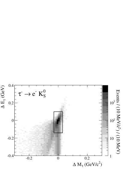
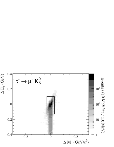
The signal candidates are then examined in the two
dimensional distribution of vs. , where
is defined as the difference between the invariant mass of the
reconstructed and the world average value Yao et al. (2006), and is
defined as the difference between the energy of the reconstructed and the expected energy, half the CM total energy.
Only candidates with a value within and a value within are retained.
The whole decay tree is then fitted requiring that,
within reconstruction uncertainties,
the decay products form a vertex,
the mass is constrained to the nominal value,
and the track and the trajectory form a vertex close to the
beam interaction region.
To improve the energy resolution, a bremsstrahlung recovery procedure is applied for the
decay mode only: before the fit, the track candidate is combined
with up to three photons with an energy
larger than 30 and contained in a cone around the track
direction of ,
where is the polar angle and the azimuthal angle in
the laboratory system.
The constrained fit must have a probability
larger than 1%. If more than one candidate is found
(which occurs in less than 1% of the events), only that with
the largest probability is retained.
After the above selection is applied, backgrounds remain, mainly from
Bhabha events for the electron channel and from non-lepton events for
the muon channel due to the larger pion to muon misidentification. To
improve the background rejection, further requirements are imposed on the candidates. For the muon channel, the laboratory momentum must be
greater than 1.0. For the electron channel, in order to remove
events with a photon conversion faking a , the invariant mass of the
daughters, calculated using the momentum from the fit and assigning
them the electron mass, is required to be greater than 0.10. The
flight length significance is computed as the three-dimensional
distance in the laboratory system between the vertex and the vertex, divided by its error, and we select events with a flight length
significance greater than 3.0. Finally, the reconstructed mass is
required to be between 0.482 and 0.514. The last two criteria are
included in the loose selection for the electron channel while, for the
muon channel, they are applied at a later stage in order to maintain
sufficient statistics in the loose selection sample.
The amount of background events due to dimuon and Bhabha processes
is negligible after the loose selection has been applied and
most of the surviving events come from charm decays,
such as and , and from
combinations in the events of a true and a fake lepton.
To avoid bias from adapting selection requirements to the data,
the tight selection has been optimized in a blind way, without looking at the data
in the rectangular region (blinded box) shown in Fig. 1,
corresponding to more than times the resolution for signal events
on and , respectively.
Figure 1: Candidate distributions for signal MC samples (top)
and (bottom) in the (, )
plane after the loose selection. The rectangle corresponds to the blinded box.
The -axis scale is logarithmic.
As discussed above, selection criteria have been chosen to optimize the sensitivity on the upper limit.
Therefore, for the tight selection the tighter PID selectors
plus the following requirements are applied.
The event’s missing momentum is computed by subtracting from the momentum all track candidates and all unmatched calorimeter energy deposits.
To reject events with tracks and photons lost out of the acceptance,
the missing momentum is required to have a transverse
component greater than 0.1 (0.2) for the electron (muon) channel
and the cosine of its polar angle in the laboratory system must be smaller than 0.95.
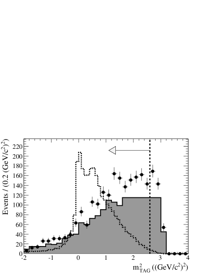
In a pair event, when neglecting radiation, the tag-side has
the same momentum as the signal-side but the opposite direction.
In addition, assuming that the tag decays to a one neutrino (hadronic) mode,
the event’s missing momentum corresponds to the neutrino momentum.
These two assumptions determine the tag 4-momentum , and
the neutrino 4-momentum , respectively, and we define the
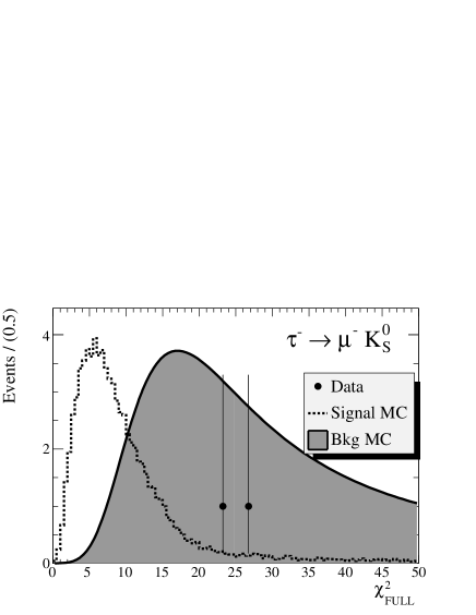
squared invariant mass as .
As shown in Fig. 2, peaks at small values
for signal events
and extends to higher values for background events.
Figure 2: Distributions of after the loose selection
for the channel.
The data distribution is shown by solid circles with error bars, background MC
with a filled histogram
and signal MC with a dashed line.
The signal MC distribution is normalized arbitrarily, while the background MC is normalized
to the data luminosity. The vertical dashed line and the arrow indicate the applied requirement.
The tail on the right for the signal sample is due to tag decays
to (leptonic) modes with two neutrinos, while the tail
on the left for the background sample is due
to events with missing energy from lost photons or tracks.
The variable is required to be smaller than 2.6 for both channels.
Shapes for data and MC agree within error but a discrepancy is observed in the normalization.
This does not affect the results because the final number of background events
is obtained using the data sample.
The background events are further reduced by requiring less than six photons on the tag side.
Signal events have missing momentum due only to
the undetected neutrino(s) from the tagging decay.
Therefore, only for the channel,
the cosine of the angle between the missing momentum and the signal candidate is required to be negative,
to further reject non-leptonic backgrounds and improve the sensitivity.
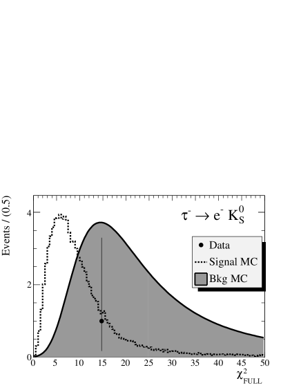
For the final step of analysis, we define another discriminating variable,
, as the of the geometrical and kinematical fit for
the whole decay tree, with additional constraints of and equal to 0.
Most signal events have values in the range 0-50,
and we consider this range in the following.
In Fig. 3 we show the distributions of for data and
signal MC inside the blinded box after the tight selection.
An analytic curve describing the background, as detailed in the following, is also
presented.
Figure 3: Distributions of after the tight selection
for the (top) and (bottom) channel.
The data events are shown by solid circles with error bars.
The signal MC distributions are shown by dashed lines, while
the background shapes are shown with filled histograms.
The signal and background MC distributions are normalized arbitrarily.
The overall efficiency in this range of ,
after the tight selection, and inside the blinded box
is for the mode and for the mode.
The total signal efficiency is estimated by dividing the number of
selected signal MC events by the total number of generated decays
and includes the BF.
We estimate the number of background events in the signal region using
the number of MC background events in the range 0-50 of after
the loose selection multiplied by the ratio of numbers of MC background
events after tight and loose selections in the full range of .
We apply a 10% correction to normalize the MC to the levels
of background seen in data outside the blinded box after the tight selection.
Total backgrounds of and events are expected for and respectively.
Finally the signal region is unblinded and and events
are found for electron and muon modes, respectively, as already shown
in Fig. 3.
Since no excess above the expected background level is found,
90% confidence level limits have been determined
according to the modified frequentist analysis (or method) Junk (1999); Jam (2000).
This method is more powerful than a simple UL estimation based on numbers of observed and expected events
as it takes into account the different distributions of one or more discriminating variables
between signal and background.
The discriminating variable used in this analysis is .
The signal distribution is simply provided by the MC sample as already shown
in Fig. 3, but this cannot be done for the background as too
few events survive the tight selection, but also the loose one.
Therefore we obtain smooth background shapes by fitting the product
of a Landau function and a straight line to the MC background
distributions after the loose selection.
Any distortions on the shapes that could be introduced by the tight selection
are negligible compared to the uncertainties of the shapes themselves.
The resulting curves are presented in Fig. 3.
The adopted test-statistic is the likelihood ratio
, where and
are, respectively, the likelihood to find the
observed events in the hypothesis of background only and of background plus
a given amount of signal. The latter, and consequently ,
are functions of the hypothesized signal BF.
The confidence level is defined as the ratio ,
where and are estimated using an ensemble of simulated
datasets, generated from signal plus background or background only.
The generation is iterated with a varying hypothetical value of the
number of signal events, depending on the BF. and are then
the probabilities that the test-statistic would be less than the
values observed in data, under the respective hypothesis.
Signal hypotheses corresponding to are rejected
at the confidence level.
This method
avoids that a negative fluctuation of the background is translated
into a large improvement of the exclusion limit and allows to include
uncertainties directly on signal and background distributions.
The ULs on BFs at 90% confidence level are calculated as
(1)
where is the limit for the signal yield at 90% confidence level, and
and are already defined above.
The dominant systematic uncertainties on the signal efficiency for the electron (muon)
channel come from possible data/MC differences in the efficiency of the PID requirements,
0.4% (5.1%) and of the tracking reconstruction, 1.7% (1.6%).
Other sources of systematic uncertainty for the efficiency are:
data/MC differences in reconstruction efficiency (1.0%),
the beam energy scale and the energy spread (less than 0.2%).
The efficiency errors from MC statistics are negligible compared with the systematics ones.
The uncertainty for the total number of pairs comes from
the error on the luminosity and on the cross section values (0.7%).
We assume these uncertainties are uncorrelated and combine them
in quadrature to give a total signal uncertainty of
2.1% and 5.5% respectively for the electron and muon channels.
For each bin of the signal distribution, we consider the total
uncertainties on the signal yield, and for the background distributions the
uncertainties on the expected background levels.
The uncertainties are treated as fully correlated between the bins as they are mainly
due to normalization uncertainties.
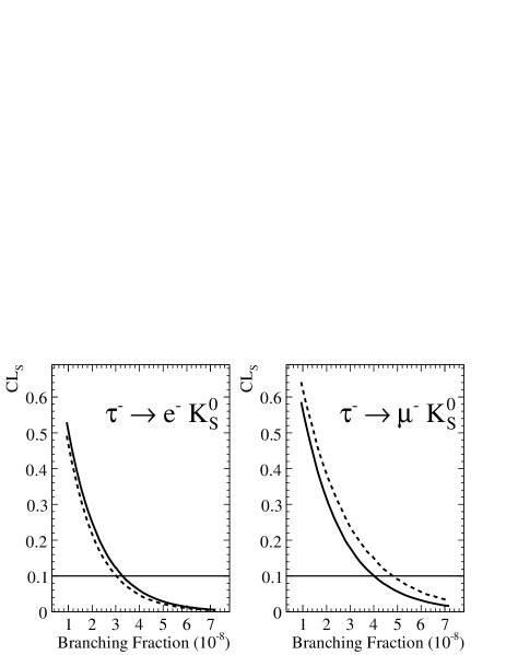
The analysis results are summarized in Fig. 4 presenting
for the observed events versus the BFs,
with the horizontal line defining the UL at 90% confidence level.
Figure 4: Observed (full line) and expected (dashed line) as a function
of the BFs () for the decays and .
From Fig. 4, the ULs on the BFs
at 90% confidence level are determined to be:
and .
The obtained using the number of expected background MC events, instead
of data, are shown in the same figure and the BF values at 90% confidence level
can be regarded as the sensitivities:
for the electron channel and for the muon one.
ULs are also determined by exploiting another technique that
gives a similar but worse sensitivity for the UL, so it is used only as cross-check.
For this method, selection criteria on the same quantities
were slightly tightened to reduce the background
as much as possible, and
signal candidates are counted inside the elliptical
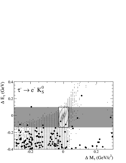
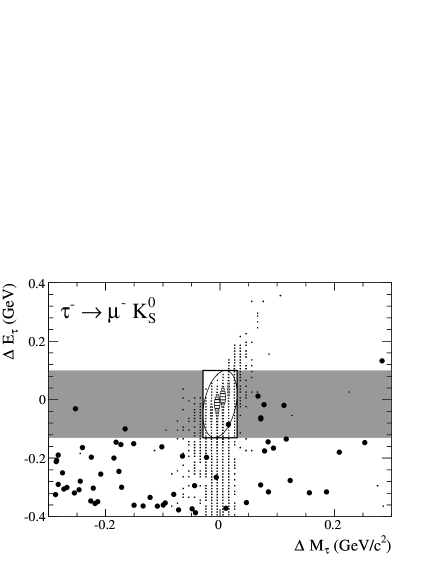
region shown in Fig. 5.
Figure 5: Candidate distribution in the (, ) plane after all
selections for cross-check method ( on the top, on the
bottom). Data candidates are indicated by solid circles.
The boxes show the signal MC distribution with arbitrary normalization.
The blinded box, used for both methods, corresponds to the rectangle.
The gray bands and the ellipse
indicate the sidebands used for extrapolating the background and the signal region
for the cross-check measurement.
The -axis scale is linear.
The final signal efficiencies with these selections are
for the mode and for the mode.
The level of background in the signal ellipse is estimated by
extrapolating the event densities found in two sideband regions of ,
as defined in Fig. 5.
The background distribution is modeled as a linear function
plus a Gaussian function to account for the peak related
to the decay mode . This is fitted
at the loose selection stage, where there are
sufficient statistics in the sidebands to estimate the shape.
Then the fitted background distribution is normalized according to the
number of data events in the sidebands after the tight selection.
The final estimated number of background events in the signal region is
and for the electron and muon channels respectively, where the last number is the
systematic uncertainty accounting for the observed differences between
estimated and real MC sample events inside the signal region
at the loose selection stage.
When the signal region is unblinded, we find inside the elliptical
signal region only one event for each channel.
Using the signal efficiencies, the estimated residual backgrounds,
and the number of observed events
ULs on the BFs at 90% confidence level for this cross-check
are calculated with the POLE program Conrad et al. (2003).
Uncertainties are included assuming that efficiency and
background values have a Gaussian distribution, and that they are not correlated.
The resulting ULs are and .
In conclusion, a search for the lepton flavour violating decays has been
performed using a data sample of collected with the BABAR detector
at the SLAC PEP-II electron-positron storage rings.
No statistically significant excess of events is observed in either channel and
the resulting ULs are and at 90% confidence level.
These results are the most restrictive ULs on the BFs
of these decay modes, and can be used to constrain parts of
the theoretical phase space in several models of physics beyond the
Standard Model.
We are grateful for the
extraordinary contributions of our PEP-II colleagues in
achieving the excellent luminosity and machine conditions
that have made this work possible.
The success of this project also relies critically on the
expertise and dedication of the computing organizations that
support BABAR.
The collaborating institutions wish to thank
SLAC for its support and the kind hospitality extended to them.
This work is supported by the
US Department of Energy
and National Science Foundation, the
Natural Sciences and Engineering Research Council (Canada),
the Commissariat à l’Energie Atomique and
Institut National de Physique Nucléaire et de Physique des Particules
(France), the
Bundesministerium für Bildung und Forschung and
Deutsche Forschungsgemeinschaft
(Germany), the
Istituto Nazionale di Fisica Nucleare (Italy),
the Foundation for Fundamental Research on Matter (The Netherlands),
the Research Council of Norway, the
Ministry of Education and Science of the Russian Federation,
Ministerio de Educación y Ciencia (Spain), and the
Science and Technology Facilities Council (United Kingdom).
Individuals have received support from
the Marie-Curie IEF program (European Union) and
the A. P. Sloan Foundation.
References
Marciano and Sanda (1977)
W. J. Marciano and
A. I. Sanda,
Phys. Lett. B 67,
303 (1977).
Lee and Shrock (1977)
B. W. Lee and
R. E. Shrock,
Phys. Rev. D 16,
1444 (1977).
Cheng and Li (1977)
T.-P. Cheng and
L.-F. Li,
Phys. Rev. D 16,
1425 (1977).
Brooks et al. (1999)
M. L. Brooks
et al. (MEGA Collaboration),
Phys. Rev. Lett. 83,
1521 (1999).
Aubert et al. (2005)
B. Aubert et al.
(BABAR Collaboration), Phys. Rev.
Lett. 95, 041802
(2005).
Aubert et al. (2006)
B. Aubert et al.
(BABAR Collaboration), Phys. Rev.
Lett. 96, 041801
(2006).
Hayasaka et al. (2008)
K. Hayasaka et al.
(Belle Collaboration), Phys. Lett.
B 666, 16
(2008).
Raidal et al. (2008)
M. Raidal et al.
(2008), eprint hep-ph/0801.1826.
(9)
eprint Charge conjugate decays are implicitly included.
Ilakovac (2000)
A. Ilakovac,
Phys. Rev. D 62,
036010 (2000).
Saha and Kundu (2002)
J. P. Saha and
A. Kundu,
Phys. Rev. D 66,
054021 (2002).
Miyazaki et al. (2006)
Y. Miyazaki et al.
(Belle Collaboration), Phys. Lett.
B 639, 159
(2006).
Aubert et al. (2002)
B. Aubert et al.
(BABAR Collaboration), Nucl.
Instrum. Meth. A 479, 1
(2002).