TUM-HEP-704/08

MPP-2008-152

Rare $K$ and $B$ Decays in a
Warped Extra Dimension with Custodial Protection

Monika Blanke^a,b, Andrzej J. Buras^a,c, Björn Duling^a,
Katrin Gemmler^a and Stefania Gori^a,b

^aPhysik Department, Technische Universität München, D-85748 Garching, Germany

^bMax-Planck-Institut für Physik (Werner-Heisenberg-Institut),
D-80805 München, Germany

^cTUM Institute for Advanced Study, Technische Universität München,
D-80333 München, Germany

We present a complete study of rare $K$ and $B$ meson decays in a warped extra dimensional model with a custodial protection of (both diagonal and non-diagonal) $Zd_{L}^{i}\bar{d}_{L}^{j}$ couplings, including $K^{+}\to\pi^{+}\nu\bar{\nu}$, $K_{L}\to\pi^{0}\nu\bar{\nu}$, $K_{L}\to\pi^{0}\ell^{+}\ell^{-}$, $K_{L}\to\mu^{+}\mu^{-}$, $B_{s,d}\to\mu^{+}\mu^{-}$, $B\to K\nu\bar{\nu}$, $B\to K^{*}\nu\bar{\nu}$ and $B\to X_{s,d}\nu\bar{\nu}$. In this model in addition to Standard Model one loop contributions these processes receive tree level contributions from the $Z$ boson and the new heavy electroweak gauge bosons. We analyse all these contributions that turn out to be dominated by tree level $Z$ boson exchanges governed by right-handed couplings to down-type quarks. Imposing all existing constraints from $\Delta F=2$ transitions analysed by us recently and fitting all quark masses and CKM mixing parameters we find that a number of branching ratios for rare $K$ decays can differ significantly from the SM predictions, while the corresponding effects in rare $B$ decays are modest, dominantly due to the custodial protection being more effective in $B$ decays than in $K$ decays. In order to reduce the parameter dependence we study correlations between various observables within the $K$ system, within the $B$ system and in particular between $K$ and $B$ systems, and also between $\Delta F=2$ and $\Delta F=1$ observables. These correlations allow for a clear distinction between this new physics scenario and models with minimal flavour violation or the Littlest Higgs Model with T-parity, and could give an opportunity to future experiments to confirm or rule out the model. We show how our results would change if the custodial protection of $Zd_{L}^{i}\bar{d}^{j}_{L}$ couplings was absent. In the case of rare $B$ decays the modifications are spectacular.

1 Introduction

In a recent paper [1] we have presented a complete study of $\Delta S=2$ and $\Delta B=2$ processes in a Randall-Sundrum (RS) [2] model with an extended gauge group and the custodial $P_{LR}$ symmetry that has been constructed to protect the $T$ parameter and the coupling $Zb_{L}\bar{b}_{L}$ from new physics (NP) tree level contributions [3, 4, 5]. In this context we have pointed out [1] that this custodial symmetry automatically protects flavour violating $Zd_{L}^{i}\bar{d}_{L}^{j}$ couplings so that tree level $Z$ contributions to all processes in which the flavour changes appear in the down quark sector are dominantly represented by $Zd_{R}^{i}\bar{d}_{R}^{j}$ couplings.

Additional NP contributions to the decays in question in the RS model considered arise from tree level heavy electroweak gauge bosons $Z_{H}$ and $Z^{\prime}$ and KK photon $A^{(1)}$ exchanges. However the $Z^{\prime}d_{L}^{i}\bar{d}_{L}^{j}$ couplings are suppressed, similarly to $Zd_{L}^{i}\bar{d}_{L}^{j}$ couplings, by the custodial symmetry, and $A^{(1)}$ contributions are suppressed by the electromagnetic coupling constant $e^{\text{4D}}$ and the electric charge $Q=-1/3$ of down-type quarks. Consequently only $Z_{H}$ contributions are really relevant. They played a prominent role in $\Delta B=2$ observables considered in [1] but had to compete there with the KK gluon exchanges. The latter contributions are absent at tree level in $\Delta F=1$ decays with leptons in the final state and consequently at first sight one would expect that rare $K$ and $B$ decays are governed by the physics of the $Z_{H}$ gauge boson. However, in $\Delta F=1$ processes tree level $Z$ contributions are of the same order in $v^{2}/M_{\text{KK}}^{2}$ as the contribution from $Z_{H}$, and moreover $Z$ boson couplings to leptons are ${\cal O}(1)$, whereas the ones of $Z_{H}$ and $Z^{\prime}$ are suppressed. Consequently, $Z_{H}$ has to compete this time with tree level $Z$ contributions, and as we will see below $Z$ generally wins this competition in spite of the custodial protection of its left-handed couplings to the down-type quarks. All these new effects bring in new flavour violating interactions beyond those governed by the CKM matrix and one should expect an interesting pattern of deviations from the SM and minimal flavour violation (MFV) [6, 7, 8, 9, 10] expectations.

The goal of the present paper is to extend our analysis of $\Delta F=2$ processes in [1] to rare decays of $K$ and $B_{d,s}$ mesons. In particular we will present for the first time the formulae for the branching ratios of $K^{+}\to\pi^{+}\nu\bar{\nu}$, $K_{L}\to\pi^{0}\nu\bar{\nu}$, $K_{L}\to\pi^{0}\ell^{+}\ell^{-}$, $K_{L}\to\mu^{+}\mu^{-}$, $B_{s,d}\to\mu^{+}\mu^{-}$, $B\to K\nu\bar{\nu}$, $B\to K^{*}\nu\bar{\nu}$ and $B_{s,d}\to X_{s,d}\nu\bar{\nu}$ in the warped extra dimensional model with a protective custodial symmetry. A partial study of these decays in a model without custodial protection has been done in [11, 12, 13, 14] and a more detailed analysis in the latter case is in progress [15].

Two comments should be made already at the beginning of our paper:

• It is known that the model in question cannot easily satisfy the $\varepsilon_{K}$ constraint for KK scales of order ${\cal O}(1\,{\rm TeV})$ [16]. Yet as we have demonstrated in [1] there exist regions in parameter space with only modest fine-tuning in the 5D Yukawa couplings involved, which allows to obtain a satisfactory description of the quark masses and CKM parameters and to satisfy all existing $\Delta F=2$ (in particular $\varepsilon_{K}$) and electroweak precision constraints for scales $M_{\text{KK}}\simeq 3\,{\rm TeV}$ in the reach of the LHC. In the present paper we will perform our numerical analysis for these regions of parameter space only.

• In view of many free parameters in the model in question we will search for correlations between various observables with the hope that these correlations will be less parameter dependent than the individual observables themselves. Such correlations can originate from the fact that the quark shape functions enter various processes universally.

Our paper is organised as follows. In Section 2 we summarise briefly those ingredients of the model in question that we will need in our analysis. A very detailed presentation of the model is presented in [18]. In Section 3 we derive the formulae for the effective Hamiltonians governing $s\to d\nu\bar{\nu}$, $b\to q\nu\bar{\nu}$, $s\to d\ell^{+}\ell^{-}$ and $b\to q\ell^{+}\ell^{-}$ ($q=d,s$) transitions. In Section 4 we calculate the most interesting exclusive rare decay branching ratios in the $K$ and $B$ meson systems, including those for the processes $K^{+}\rightarrow\pi^{+}\nu\bar{\nu}$, $K_{L}\rightarrow\pi^{0}\nu\bar{\nu}$, $B\to K^{(*)}\nu\bar{\nu}$, $B_{s,d}\to\mu^{+}\mu^{-}$, $K_{L}\to\mu^{+}\mu^{-}$ and $K_{L}\to\pi^{0}\ell^{+}\ell^{-}$. Section 5 is dedicated to the inclusive decays $B\to X_{s,d}\nu\bar{\nu}$. In Section 6 we outline the strategy for the study of a number of correlations between various observables within the $K$ system, within the $B$ system and in particular between $K$ and $B$ systems. Sections 3–6 give formulae that are sufficiently general to be applied to every model with tree level flavour violating contributions in which heavy neutral gauge bosons have arbitrary masses and arbitrary left-handed and right-handed couplings. Moreover several ideas, in particular related to correlations between various observables are applicable to all extensions of the SM. In Section 7, before entering the numerical analysis, we present the anatomy of NP contributions in the model in question that reveals a particular pattern of deviations from the SM. In Section 8 a detailed numerical analysis of these branching ratios is presented. In particular we study the correlations not only between various $\Delta F=1$ observables but also between $\Delta F=1$ and $\Delta F=2$ observables. Of interest is the question whether the large values of $A_{\text{CP}}(B_{s}\to\psi\phi)$ and $A^{s}_{\text{SL}}$ found in [1] can still be found simultaneously with large effects in rare decay branching ratios. We summarise our results in Section 9. Few technicalities are relegated to appendices.

2 The Model

2.1 Preliminaries

The aim of this section is to briefly review the most important ingredients of the model under consideration. A detailed theoretical discussion is presented in [18].

The starting point is the Randall-Sundrum (RS) geometric background, i. e. a 5D spacetime, where the extra dimension is restricted to the interval $0\leq y\leq L$, with a warped metric given by [2]

$$ds^{2}=e^{-2ky}\eta_{\mu\nu}dx^{\mu}dx^{\nu}-dy^{2}\,.$$ (2.1)

Here the curvature scale $k$ is assumed to be $k\sim{\cal O}(M_{\text{Pl}})$. Due to the exponential warp factor $e^{-ky}$, the effective energy scales depend on the position $y$ along the extra dimension, so that with $e^{kL}=10^{16}$ the gauge hierarchy problem can be solved. In what follows we will therefore treat

$$f=ke^{-kL}\sim{\cal O}(\text{TeV})$$ (2.2)

as the only free parameter coming from space-time geometry. In our numerical analysis we will use $f=1\,{\rm TeV}$.

In order to avoid stringent constraints from electroweak precision observables, all gauge and matter fields are assumed to live in the 5D bulk [19, 20, 21], while the Higgs boson is confined to the IR brane at $y=L$.

2.2 Electroweak Gauge Sector

The minimal RS model with bulk fields and the SM gauge group in the bulk turns out to be severely constrained by EW precision data and in particular by the $T$ parameter, so that the first KK excitations have to be as heavy as $M_{\text{KK}}\sim{\cal O}(10\,{\rm TeV})$ and would consequently be beyond the reach of the LHC [3, 22].

However such dangerous contribution to the $T$ parameter and also to the $Zb_{L}\bar{b}_{L}$ coupling can be avoided by enlarging the bulk symmetry to [3, 4, 5]

$$G_{\text{bulk}}=SU(3)_{c}\times SU(2)_{L}\times SU(2)_{R}\times U(1)_{X}\times P_{LR}\,.$$ (2.3)

Here the discrete exchange symmetry

$$P_{LR}:SU(2)_{L}\leftrightarrow SU(2)_{R}$$ (2.4)

has been introduced in order to suppress the non-universal corrections to the $Zb_{L}\bar{b}_{L}$ vertex. Details on particular fermion embeddings respecting that symmetry can be found e. g. in [5, 23, 24, 18].

From the enlarged gauge group and the first excited KK modes of the SM electroweak gauge bosons that we include in our analysis there arise three new neutral electroweak gauge bosons,

$$Z_{H}\,,\qquad Z^{\prime}\,,\qquad A^{(1)}$$ (2.5)

in addition to the SM $Z$ boson and photon, where the first two are linear combinations of the gauge eigenstates $Z^{(1)}$ and $Z_{X}^{(1)}$ [18]. Neglecting small $SU(2)_{R}$ breaking effects on the UV brane ($y=0$) and corrections due to EW symmetry breaking, one finds

$$M_{Z_{H}}=M_{Z^{\prime}}=M_{A^{(1)}}\equiv M_{\text{KK}}\simeq 2.45f\,.$$ (2.6)

All KK gauge bosons are localised close to the IR brane, inducing tree level FCNCs, as discussed in more detail in Section 2.3.3.

The RS model with custodial protection of  $T$ and $Zb_{L}\bar{b}_{L}$ as described above and mildly constrained quark shape functions then turns out to be consistent with EW precision observables for KK scales as low as $M_{\text{KK}}\simeq(2-3)\,{\rm TeV}$ [25, 26].

2.3 Fermion Sector

2.3.1 Zero Mode Localisation

Bulk fermions in the RS background offer a natural explanation of the observed hierarchies in fermion masses and mixings [21, 19, 27]. At the same time a powerful suppression mechanism for flavour changing neutral current (FCNC) interactions, the so-called RS-GIM mechanism, is provided [13].

The bulk profile of a fermionic zero mode depends strongly on its bulk mass parameter $c_{\Psi}$. In case of a left-handed zero mode $\Psi_{L}^{(0)}$ it is given by

$$f^{(0)}_{L}(y,c_{\Psi})=\sqrt{\frac{(1-2c_{\Psi})kL}{e^{(1-2c_{\Psi})kL}-1}}e^{-c_{\Psi}ky}$$ (2.7)

with respect to the warped metric. Therefore, for $c_{\Psi}>1/2$ the fermion $\Psi_{L}^{(0)}$ is localised towards the UV brane and exponentially suppressed on the IR brane, while for $c_{\Psi}<1/2$ it is localised towards the IR brane. The bulk profile for a right-handed zero mode $\Psi_{R}^{(0)}$ can be obtained from

$$f^{(0)}_{R}(y,c_{\Psi})=f^{(0)}_{L}(y,-c_{\Psi})\,,$$ (2.8)

so that its localisation depends on whether $c_{\Psi}<-1/2$ or $c_{\Psi}>-1/2$. Note that as in the SM the left- and right-handed zero modes present in the spectrum necessarily belong to different 5D multiplets, so that generally $c_{\Psi_{L}}\neq c_{\Psi_{R}}$.

In order to preserve the discrete $P_{LR}$ symmetry, we embed the left handed SM quarks into bidoublets of $SU(2)_{L}\times SU(2)_{R}$, while the right handed up and down quarks belong to $(\mathbf{1},\mathbf{1})$ and $(\mathbf{1},\mathbf{3})\oplus(\mathbf{3},\mathbf{1})$ representations, respectively [23, 18]. Their bulk mass parameters are denoted by $c_{Q}^{i}$, $c_{u}^{i}$ and $c_{d}^{i}$, respectively.

2.3.2 Higgs Field and Yukawa Couplings

As the Higgs boson in our model is localised on the IR brane, the effective 4D Yukawa couplings, relevant for the SM fermion masses and mixings, read

$$Y^{u,d}_{ij}=\lambda^{u,d}_{ij}\,\frac{e^{kL}}{kL}f^{(0)}_{L}(y=L,c_{Q}^{i})f^{(0)}_{R}(y=L,c_{u,d}^{j})\equiv\lambda^{u,d}_{ij}\,\frac{e^{kL}}{kL}f^{Q}_{i}f^{u,d}_{j}\,,$$ (2.9)

where $\lambda^{u,d}$ are the fundamental 5D Yukawa coupling matrices. In order to preserve perturbativity of the model, we require as usual $|\lambda^{u,d}_{ij}|\leq 3$. Here and in the following we work in the special basis in which the bulk mass matrices are taken to be real and diagonal. Such a basis can always be reached by appropriate unitary transformations in the $Q_{i}$, $u_{i}$ and $d_{i}$ sectors.

Note that the strong hierarchies of quark masses and mixings can be traced back to ${\cal O}(1)$ bulk mass parameters and anarchic 5D Yukawa couplings $\lambda^{u,d}$ due to the exponential dependence of $Y^{u,d}$ on the bulk mass parameters $c_{Q,u,d}$. The flavour structure then resembles the one of models with a Froggatt-Nielsen symmetry [28], so that with the help of the latter paper analytic formulae for quark masses and flavour mixing matrices $\mathcal{U}_{L},\mathcal{U}_{R},\mathcal{D}_{L},\mathcal{D}_{R}$ and the CKM matrix

$$V_{\text{CKM}}=\mathcal{U}_{L}^{\dagger}\mathcal{D}_{L}$$ (2.10)

can be obtained [1, 22].

Due to the mixing with heavy KK fermions flavour violating Higgs couplings are induced already at tree level. However it can straightforwardly be shown [1] that these couplings receive a strong chirality suppression in addition to the usual RS-GIM suppression and are therefore negligibly small.

2.3.3 Flavour Violation by Neutral Electroweak Gauge Bosons

As a consequence of the exponential localisation of the gauge KK modes towards the IR brane, their couplings to zero mode fermions are not flavour universal, but depend strongly on the relevant bulk mass parameter $c_{Q,u,d}^{i}$. After rotation to the fermion mass eigenbasis then FCNC couplings of the heavy gauge bosons $Z_{H}$, $Z^{\prime}$ and $A^{(1)}$ are induced. They can be parameterised by the coupling matrices $\hat{\Delta}_{L}(V)$ and $\hat{\Delta}_{R}(V)$ ($V=Z_{H},Z^{\prime},A^{(1)}$), that have been evaluated in [1] and are collected for completeness in Appendix A.

Moreover, due to the mixing of the SM $Z$ boson with the heavy KK modes $Z^{(1)}$ and $Z^{(1)}_{X}$, also the $Z$ boson couplings become flavour violating already at the tree level. An additional contribution arises from the mixing of the zero mode fermions with their heavy KK partners.

On the other hand, it has been observed in [1] that the custodial protection symmetry $P_{LR}$, originally introduced to protect the $Zb_{L}\bar{b}_{L}$ coupling, removes not only the non-universal contributions to that coupling, but at the same time efficiently protects all tree level $Zd^{i}_{L}\bar{d}^{j}_{L}$ couplings, so that at the tree level the $Z$ boson couplings to left-handed down type quarks are strongly suppressed. We note that the protective $P_{LR}$ symmetry is at work not only for the interplay of $Z^{(1)}$ and $Z^{(1)}_{X}$ contributions to the $Z$ and $Z^{\prime}$ couplings, but also for the KK fermion contributions. This is because the fermion sector has been constructed in a $P_{LR}$-invariant manner as well and the left-handed down-type quarks transform as $P_{LR}$-eigenstates. The protective symmetry is however not active for right-handed quarks, so that flavour violating $Zd^{i}_{R}\bar{d}^{j}_{R}$ couplings are important already at the tree level.

While $Z$ boson contributions to $\Delta F=1$ decays are parametrically enhanced with respect to the contributions of $Z_{H}$, $Z^{\prime}$ and $A^{(1)}$ by a factor $kL\sim 35$ [13, 22], they are suppressed by the fact that flavour violation is generally weaker in the right-handed sector. In spite of this we will see in Sections 7 and 8 that $Z$ boson contributions are larger than the contributions of $Z_{H},Z^{\prime}$ and $A^{(1)}$.

We note that the strength of RS flavour violation depends on the presence of possible brane kinetic terms which alter the matching relation between 5D and 4D gauge couplings, see [16, 29, 1] for details. In order not to complicate the present analysis we assume the simple intermediate scenario in which the tree level matching condition $g^{\text{4D}}=g^{\text{5D}}/\sqrt{L}$ holds. A generalisation of our analysis to include deviations from this ansatz is straightforward.

3 Basic Formulae for Effective Hamiltonians

3.1 Preliminaries

The goal of the present section is to give formulae for the effective Hamiltonians relevant for rare $K$ and $B$ decays that in addition to SM one-loop contributions include tree level contributions from the SM $Z$ gauge boson and the heavy gauge bosons $Z_{H}$, $Z^{\prime}$ and $A^{(1)}$. It will be useful to first keep our presentation as general as possible so that the formulae given below could be applied to all other models with tree level flavour violating contributions in which the heavy neutral gauge bosons have arbitrary masses and arbitrary left-handed and right-handed couplings. Subsequently, we will apply these formulae to our model in which at leading order the three new heavy electroweak gauge bosons are degenerate in mass and certain simplifications occur.

Our presentation includes the contributions from all operators originating only from tree level exchanges of electroweak gauge bosons. Consequently we do not discuss the dipole operators that enter effective Hamiltonians first at the one-loop level. We will return to them in the context of the model in question in a separate publication. This implies that the effective Hamiltonians for $b\to d\ell^{+}\ell^{-}$ and $b\to s\ell^{+}\ell^{-}$ transitions given below are incomplete and we cannot perform yet the phenomenology of decays like $B\to K^{*}\ell^{+}\ell^{-}$, $B\to X_{s,d}\ell^{+}\ell^{-}$ and $B\to X_{s,d}\gamma$ that is left for the future.

3.2 Effective Hamiltonian for $s\to d\nu\bar{\nu}$

The effective Hamiltonian for $s\rightarrow d\nu\bar{\nu}$ transitions is given in the SM as follows

$$\left[{\cal H}_{\text{eff}}^{\nu\bar{\nu}}\right]^{K}_{\text{SM}}=g_{\text{SM}}^{2}\sum_{\ell=e,\mu,\tau}{\left[\lambda_{c}^{(K)}{X_{\text{NNL}}^{\ell}(x_{c})}+\lambda_{t}^{(K)}X(x_{t})\right]}(\bar{s}d)_{V-A}(\bar{\nu}_{\ell}\nu_{\ell})_{V-A}+h.c.\,,$$ (3.1)

where $x_{i}=m_{i}^{2}/M_{W}^{2}$, $\lambda_{i}^{(K)}=V_{is}^{*}V_{id}$ and $V_{ij}$ are the elements of the CKM matrix. $X_{\text{NNL}}^{\ell}(x_{c})$ and $X(x_{t})$ comprise internal charm and top quark contributions, respectively. They are known to high accuracy including QCD corrections [30, 31, 32]. For convenience we have introduced

$$g_{\text{SM}}^{2}=\frac{G_{F}}{\sqrt{2}}\frac{\alpha}{2\pi\sin^{2}\theta_{W}}\,.$$ (3.2)

In the RS model considered, $\left[{\cal H}_{\text{eff}}^{\nu\bar{\nu}}\right]^{K}$ receives tree-level contributions from $Z$ and from the heavy neutral gauge bosons $Z_{H}$ and $Z^{\prime}$ which contain new flavour violating interactions.

We begin with the FCNC Lagrangian for $Z$

$$\mathcal{L}_{\text{FCNC}}(Z)=-\left[\mathcal{L}_{L}(Z)+\mathcal{L}_{R}(Z)\right]\,,$$ (3.3)

where

$$\mathcal{L}_{L}(Z) = \Delta_{L}^{sd}(Z)\left(\bar{s}_{L}\gamma_{\mu}d_{L}\right)Z^{\mu}\,,$$ (3.4)

$$\mathcal{L}_{R}(Z) = \Delta_{R}^{sd}(Z)\left(\bar{s}_{R}\gamma_{\mu}d_{R}\right)Z^{\mu}\,,$$ (3.5)

with explicit expressions for $\Delta_{L}^{sd}(Z)$ and $\Delta_{R}^{sd}(Z)$ given in Appendix A.

For the $Z\nu\bar{\nu}$ coupling we analogously write

$$\mathcal{L}_{\nu\bar{\nu}}(Z)=-\Delta_{L}^{\nu\nu}(Z)(\bar{\nu}_{L}\gamma_{\mu}\nu_{L})Z^{\mu}$$ (3.6)

where $\Delta_{L}^{\nu\nu}(Z)$ is given in Appendix A.

Figure 1: Tree level contributions of $Z$, $Z^{\prime}$ and $Z_{H}$ to the $s\to d\nu\bar{\nu}$ effective Hamiltonian.

A straightforward calculation of the diagram in Fig. 1 results in a new contribution to $\left[{\cal H}_{\text{eff}}^{\nu\bar{\nu}}\right]^{K}$

$$\left[{\cal H}_{\text{eff}}^{\nu\bar{\nu}}\right]_{Z}^{K}=\frac{\Delta_{L}^{\nu\nu}(Z)}{M_{Z}^{2}}\left[\Delta_{L}^{sd}(Z)(\bar{s}_{L}\gamma^{\mu}d_{L})+\Delta_{R}^{sd}(Z)(\bar{s}_{R}\gamma^{\mu}d_{R})\right]\left(\bar{\nu}_{L}\gamma_{\mu}\nu_{L}\right)+h.c.\,.$$ (3.7)

The contribution of $Z^{\prime}$ and $Z_{H}$ to $\left[{\cal H}_{\text{eff}}^{\nu\bar{\nu}}\right]^{K}$ can then be obtained from (3.7) by simply replacing $Z$ by $Z^{\prime}$ and $Z_{H}$ respectively. Explicit expressions for $\Delta_{L,R}^{sd}(Z^{\prime})$, $\Delta_{L}^{\nu\nu}(Z^{\prime})$ and $\Delta_{L,R}^{sd}(Z_{H})$, $\Delta_{L}^{\nu\nu}(Z_{H})$ can be found in Appendix A.

Combining then the contributions of $Z,Z^{\prime},Z_{H}$ in (3.7) with the SM contribution in (3.1),

$$\left[{\cal H}_{\text{eff}}^{\nu\bar{\nu}}\right]^{K}=\left[{\cal H}_{\text{eff}}^{\nu\bar{\nu}}\right]^{K}_{\text{SM}}+\left[{\cal H}_{\text{eff}}^{\nu\bar{\nu}}\right]_{Z}^{K}+\left[{\cal H}_{\text{eff}}^{\nu\bar{\nu}}\right]_{Z^{\prime}}^{K}+\left[{\cal H}_{\text{eff}}^{\nu\bar{\nu}}\right]_{Z_{H}}^{K}\,,$$ (3.8)

we finally find

$$\left[{\cal H}_{\text{eff}}^{\nu\bar{\nu}}\right]^{K} = g_{\text{SM}}^{2}\sum_{\ell=e,\mu,\tau}{\left[\lambda_{c}^{(K)}{X_{\text{NNL}}^{\ell}(x_{c})}+\lambda_{t}^{(K)}X_{K}^{V-A}\right]}(\bar{s}d)_{V-A}(\bar{\nu}_{\ell}\nu_{\ell})_{V-A}$$ (3.9)

$${}+g_{\text{SM}}^{2}\sum_{\ell=e,\mu,\tau}{\left[\lambda_{t}^{(K)}X_{K}^{V}\right]}(\bar{s}d)_{V}(\bar{\nu}_{\ell}\nu_{\ell})_{V-A}+h.c.\,.$$

Here we have introduced the functions $X_{K}^{V-A}$ and $X_{K}^{V}$, generalising the structure encountered in the Littlest Higgs model with T-parity (LHT) in [33],

$$X_{K}^{V-A} = X(x_{t})+\sum_{i=Z,Z^{\prime},Z_{H}}(X_{i}^{K})^{V-A}\,,$$ (3.10)

$$X_{K}^{V} = \sum_{i=Z,Z^{\prime},Z_{H}}(X_{i}^{K})^{V}\,,$$ (3.11)

that will turn out to be useful later on. The $Z$ contributions are given as follows

$$(X_{Z}^{K})^{V-A} = \frac{1}{\lambda_{t}^{(K)}}\frac{\Delta_{L}^{\nu\nu}(Z)}{4M_{Z}^{2}g_{\text{SM}}^{2}}\left[\Delta_{L}^{sd}(Z)-\Delta_{R}^{sd}(Z)\right]\,,$$ (3.12)

$$(X_{Z}^{K})^{V} = \frac{1}{\lambda_{t}^{(K)}}\frac{\Delta_{L}^{\nu\nu}(Z)}{2M_{Z}^{2}g_{\text{SM}}^{2}}\Delta_{R}^{sd}(Z)\,,$$ (3.13)

and the $Z^{\prime}$, $Z_{H}$ contributions can be obtained from (3.12) and (3.13) by simply replacing $Z$ by $Z^{\prime}$ and $Z_{H}$ respectively.

Some comments are in order:

• In the SM only a single operator $(\bar{s}d)_{V-A}(\bar{\nu}\nu)_{V-A}$ is present. This is due to the purely left-handed structure of $SU(2)_{L}$ gauge couplings and therefore of FCNC transitions.

• In the RS model in question also the operator $(\bar{s}d)_{V}(\bar{\nu}\nu)_{V-A}$ is present, as both the $\hat{\Delta}_{L}$ and $\hat{\Delta}_{R}$ coupling matrices have non-diagonal entries. Indeed it will turn out that in most cases $\Delta_{R}^{sd}(Z)$ yields the dominant contribution.

• On the other hand in the RS model under consideration the gauge couplings of the neutrino zero modes are purely left-handed, as the right-handed neutrinos are introduced as gauge singlets [18].

• As all NP contributions have been collected in the term proportional to $\lambda_{t}^{(K)}$, $X_{\text{NNL}}^{\ell}(x_{c})$ contains only the SM contributions that are known including QCD corrections at the NNLO level [31, 32].

3.3 Effective Hamiltonian for $b\to d\nu\bar{\nu}$ and $b\to s\nu\bar{\nu}$

Let us now generalise the result obtained in the previous section to the case of $b\to d\nu\bar{\nu}$ and $b\to s\nu\bar{\nu}$ transitions. Basically only two steps have to be performed:

1. All flavour indices have to be adjusted appropriately.

2. The charm quark contribution can be safely neglected in $B$ physics, so that only

   $$\lambda_{t}^{(d)}=V_{tb}^{*}V_{td},\qquad\lambda_{t}^{(s)}=V_{tb}^{*}V_{ts}$$ (3.14)

   enter the expressions below.

The effective Hamiltonian for $b\to q\nu\bar{\nu}$ ($q=d,s$) is then given as follows:

$$\left[{\cal H}_{\text{eff}}^{\nu\bar{\nu}}\right]^{B_{q}} = g_{\text{SM}}^{2}\sum_{\ell=e,\mu,\tau}{\left[\lambda_{t}^{(q)}X_{q}^{V-A}\right]}(\bar{b}q)_{V-A}(\bar{\nu}_{\ell}\nu_{\ell})_{V-A}$$ (3.15)

$$+g_{\text{SM}}^{2}\sum_{\ell=e,\mu,\tau}{\left[\lambda_{t}^{(q)}X_{q}^{V}\right]}(\bar{b}q)_{V}(\bar{\nu}_{\ell}\nu_{\ell})_{V-A}+h.c.\,,$$

with

$$X_{q}^{V-A} = X(x_{t})+\sum_{i=Z,Z^{\prime},Z_{H}}(X_{i}^{q})^{V-A}\,,$$ (3.16)

$$X_{q}^{V} = \sum_{i=Z,Z^{\prime},Z_{H}}(X_{i}^{q})^{V}$$ (3.17)

and

$$(X_{Z}^{q})^{V-A} = \frac{1}{\lambda_{t}^{(q)}}\frac{\Delta_{L}^{\nu\nu}(Z)}{4M_{Z}^{2}g_{\text{SM}}^{2}}\left[\Delta_{L}^{bq}(Z)-\Delta_{R}^{bq}(Z)\right]\,,$$ (3.18)

$$(X_{Z}^{q})^{V} = \frac{1}{\lambda_{t}^{(q)}}\frac{\Delta_{L}^{\nu\nu}(Z)}{2M_{Z}^{2}g_{\text{SM}}^{2}}\Delta_{R}^{bq}(Z)\,.$$ (3.19)

The $Z^{\prime}$ and $Z_{H}$ contributions can be obtained from (3.18) and (3.19) by simply replacing $Z$ by $Z^{\prime}$ and $Z_{H}$ respectively. Again all relevant $\Delta_{L,R}^{bq}$ entries can be found in Appendix A.

Note that the functions $X_{K,d,s}^{V-A,V}$ depend on the quark flavours involved, through the flavour indices in the $\Delta_{L,R}^{ij}$ $(i,j=s,d,b)$ couplings and through the $1/\lambda_{t}^{(q)}$ ($q=K,d,s$) factor in front of the new RS contributions. This should be contrasted with the case of the SM where $K$, $B_{d}$ and $B_{s}$ systems are governed by a flavour-universal loop function $X(x_{t})$ and the only flavour dependence enters through the CKM factors $\lambda_{t}^{(q)}$.

3.4 Effective Hamiltonian for $s\to d\ell^{+}\ell^{-}$

Let us recall that in the SM neglecting QCD corrections the top quark contribution to the effective Hamiltonian for $s\to d\ell^{+}\ell^{-}$ reads

$$\left[\mathcal{H}_{\text{eff}}^{\ell\bar{\ell}}\right]^{K}_{\text{SM}} = -g_{\text{SM}}^{2}\left[\lambda_{t}^{(K)}Y(x_{t})\right](\bar{s}d)_{V-A}(\bar{\ell}\ell)_{V-A}$$ (3.20)

$$+4g_{\text{SM}}^{2}\sin^{2}\theta_{W}\left[\lambda_{t}^{(K)}Z(x_{t})\right](\bar{s}d)_{V-A}(\bar{\ell}\ell)_{V}+h.c.$$

Here $Y(x_{t})$ and $Z(x_{t})$ are one-loop functions, analogous to $X(x_{t})$, that result from various penguin and box diagrams. The charm contributions and QCD corrections are irrelevant for the discussion presented below and will be included only in the numerical analysis later on. We also remark that in principle also dipole operators could be included here, but that in $K$ decays, as discussed in [34], they can be fully neglected. Finally, the operator basis chosen in (3.20) differs from the one used to study QCD corrections [34] but is very suitable for the discussion of modifications of the functions $Y(x_{t})$ and $Z(x_{t})$ due to NP contributions which we will discuss next.

Also in this case, $\left[\mathcal{H}_{\text{eff}}^{\ell\bar{\ell}}\right]^{K}$ receives tree level contributions of the gauge bosons $Z$, $Z^{\prime}$ and $Z_{H}$, and as now charged leptons appear in the final state, also the KK photon $A^{(1)}$ contributes.

Figure 2: Tree level contributions of $Z,Z^{\prime},Z_{H}$ and $A^{(1)}$ to the $s\to d\ell^{+}\ell^{-}$ effective Hamiltonian.

The relevant Feynman diagrams, shown in Fig. 2, contain on the l. h. s. the same vertices which we already encountered in the case of the $s\to d\nu\bar{\nu}$ decay. The relevant FCNC Lagrangian for $Z\bar{s}d$ couplings has been given in (3.3). For the $\ell^{+}\ell^{-}$ vertex we write in analogy to (3.6)

$$\mathcal{L}_{\ell\bar{\ell}}(Z)=-\left[\Delta_{L}^{\ell\ell}(Z)(\bar{\ell}_{L}\gamma_{\mu}\ell_{L})+\Delta_{R}^{\ell\ell}(Z)(\bar{\ell}_{R}\gamma_{\mu}\ell_{R})\right]Z^{\mu}\,.$$ (3.21)

The relevant entries have been collected in Appendix A.

The evaluation of the $Z$-exchange in Fig. 2 gives then

$$\left[{\cal H}_{\text{eff}}^{\ell\bar{\ell}}\right]_{Z}^{K} = \frac{1}{M_{Z}^{2}}\left[\Delta_{L}^{bs}(Z)(\bar{s}_{L}\gamma^{\mu}d_{L})+\Delta_{R}^{bs}(Z)(\bar{s}_{R}\gamma^{\mu}d_{R})\right]$$ (3.22)

$$\hskip 42.67912pt\cdot\left[\Delta_{L}^{\ell\ell}(Z)(\bar{\ell}_{L}\gamma_{\mu}\ell_{L})+\Delta_{R}^{\ell\ell}(Z)(\bar{\ell}_{R}\gamma_{\mu}\ell_{R})\right]+h.c.\,,$$

which contains additional operators relative to (3.20). The exchange of $Z^{\prime}$, $Z_{H}$ and $A^{(1)}$ gauge bosons yields analogous contributions that can simply be obtained from (3.22) by replacing $Z$ by $Z^{\prime}$, $Z_{H}$ and $A^{(1)}$, respectively.

Following the previous discussion, we find that the effective Hamiltonian governing $s\to d\ell^{+}\ell^{-}$ transitions can be written in the compact form

$$\left[\mathcal{H}_{\text{eff}}^{\ell\bar{\ell}}\right]^{K} = -g_{\text{SM}}^{2}\left[\lambda_{t}^{(K)}Y_{K}^{V-A}\right](\bar{s}d)_{V-A}(\bar{\ell}\ell)_{V-A}$$ (3.23)

$$+4g_{\text{SM}}^{2}\sin^{2}\theta_{W}\left[\lambda_{t}^{(K)}Z_{K}^{V-A}\right](\bar{s}d)_{V-A}(\bar{\ell}\ell)_{V}$$

$$-g_{\text{SM}}^{2}\left[\lambda_{t}^{(K)}Y_{K}^{V}\right](\bar{s}d)_{V}(\bar{\ell}\ell)_{V-A}$$

$$+4g_{\text{SM}}^{2}\sin^{2}\theta_{W}\left[\lambda_{t}^{(K)}Z_{K}^{V}\right](\bar{s}d)_{V}(\bar{\ell}\ell)_{V}+h.c.\,,$$

where we have introduced the functions $Y_{K}^{V-A,V}$ and $Z_{K}^{V-A,V}$ defined as:

$$Y_{K}^{V-A} = Y(x_{t})+\sum_{i=Z,Z^{\prime},Z_{H},A^{(1)}}(Y_{i}^{K})^{V-A}\,,$$ (3.24)

$$Z_{K}^{V-A} = Z(x_{t})+\sum_{i=Z,Z^{\prime},Z_{H},A^{(1)}}(Z_{i}^{K})^{V-A}\,,$$ (3.25)

$$Y_{K}^{V} = \sum_{i=Z,Z^{\prime},Z_{H},A^{(1)}}(Y_{i}^{K})^{V}\,,$$ (3.26)

$$Z_{K}^{V} = \sum_{i=Z,Z^{\prime},Z_{H},A^{(1)}}(Z_{i}^{K})^{V}\,,$$ (3.27)

where

$$(Y_{Z}^{K})^{V-A} = -\frac{1}{\lambda_{t}^{(K)}}\frac{\left[\Delta_{L}^{\ell\ell}(Z)-\Delta_{R}^{\ell\ell}(Z)\right]}{4M_{Z}^{2}g_{\text{SM}}^{2}}\left[\Delta_{L}^{sd}(Z)-\Delta_{R}^{sd}(Z)\right]\,,\qquad$$ (3.28)

$$(Z_{Z}^{K})^{V-A} = \frac{1}{\lambda_{t}^{(K)}}\frac{\Delta_{R}^{\ell\ell}(Z)}{8M_{Z}^{2}g_{\text{SM}}^{2}\sin^{2}\theta_{W}}\left[\Delta_{L}^{sd}(Z)-\Delta_{R}^{sd}(Z)\right]\,,$$ (3.29)

$$(Y_{Z}^{K})^{V} = -\frac{1}{\lambda_{t}^{(K)}}\frac{\left[\Delta_{L}^{\ell\ell}(Z)-\Delta_{R}^{\ell\ell}(Z)\right]}{2M_{Z}^{2}g_{\text{SM}}^{2}}\Delta_{R}^{sd}(Z)\,,$$ (3.30)

$$(Z_{Z}^{K})^{V} = \frac{1}{\lambda_{t}^{(K)}}\frac{\Delta_{R}^{\ell\ell}(Z)}{4M_{Z}^{2}g_{\text{SM}}^{2}\sin^{2}\theta_{W}}\Delta_{R}^{sd}(Z)\,.$$ (3.31)

The $Z^{\prime}$, $Z_{H}$ and $A^{(1)}$ contributions can be straightforwardly obtained from (3.28)–(3.31) by simply replacing $Z$ by $Z^{\prime}$, $Z_{H}$ and $A^{(1)}$, respectively.

3.5 Effective Hamiltonian for $b\to d\ell^{+}\ell^{-}$ and $b\to s\ell^{+}\ell^{-}$

Also in this case the effective Hamiltonian for $b\to q\ell^{+}\ell^{-}$ ($q=d,s$) can straightforwardly be obtained from (3.23) by properly adjusting all flavour indices. In addition, in contrast to the $s\to d\ell^{+}\ell^{-}$ transition, now also the dipole operator contributions mediating the decay $b\to s\gamma$ become relevant. The new RS contributions to the corresponding operators $\mathcal{Q}_{7\gamma}$ and $\mathcal{Q}_{8G}$ appear first at the one-loop level and consequently as already stated above are beyond the scope of this paper. Explicit formulae for these contributions will be presented elsewhere. In the following we will denote the total contribution of the dipole operators to the effective Hamiltonian in question simply by ${\cal H}_{\text{eff}}(b\to s\gamma)$.

Adapting then the formula in (3.23) to the present case, we find ($q=d,s$)

$$\left[\mathcal{H}_{\text{eff}}^{\ell\bar{\ell}}\right]^{B_{q}} = {\cal H}_{\text{eff}}(b\to s\gamma)-g_{\text{SM}}^{2}\left[\lambda_{t}^{(q)}Y_{q}^{V-A}\right](\bar{b}q)_{V-A}(\bar{\ell}\ell)_{V-A}-g_{\text{SM}}^{2}\left[\lambda_{t}^{(q)}Y_{q}^{V}\right](\bar{b}q)_{V}(\bar{\ell}\ell)_{V-A}$$ (3.32)

$$+4g_{\text{SM}}^{2}\sin^{2}\theta_{W}\left[\lambda_{t}^{(q)}Z_{q}^{V-A}\right](\bar{b}q)_{V-A}(\bar{\ell}\ell)_{V}+4g_{\text{SM}}^{2}\sin^{2}\theta_{W}\left[\lambda_{t}^{(q)}Z_{q}^{V}\right](\bar{b}q)_{V}(\bar{\ell}\ell)_{V}$$

$$+h.c.\,.$$

In analogy to $Y_{K}^{V-A,V},Z_{K}^{V-A,V}$ in (3.24)–(3.31), the relevant functions can be obtained from the latter formulae by replacing $K$ by $q$. The same comment applies for the contributions of $Z^{\prime}$, $Z_{H}$ and $A^{(1)}$.

4 Exclusive Rare Decays

4.1 $K^{+}\rightarrow\pi^{+}\nu\bar{\nu}$ and $K_{L}\rightarrow\pi^{0}\nu\bar{\nu}$

Having at hand the effective Hamiltonian for $s\to d\nu\bar{\nu}$ transitions derived in Section 3.2 it is now straightforward to obtain explicit expressions for the branching ratios $Br(K^{+}\rightarrow\pi^{+}\nu\bar{\nu})$ and $Br(K_{L}\rightarrow\pi^{0}\nu\bar{\nu})$. Reviews of these two decays can be found in [35, 36, 37].

As mentioned already in Section 3.2, now in addition to the usual SM operator $(\bar{s}d)_{V-A}(\bar{\nu}\nu)_{V-A}$ also the operator $(\bar{s}d)_{V}(\bar{\nu}\nu)_{V-A}$ is present. Therefore both matrix elements $\left<\pi^{+}|(\bar{s}d)_{V-A}|K^{+}\right>$ and $\left<\pi^{+}|(\bar{s}d)_{V}|K^{+}\right>$ have to be evaluated. Fortunately, as both $K^{+}$ and $\pi^{+}$ are pseudoscalar mesons, only the vector current part contributes and we simply have

$$\left<\pi^{+}|(\bar{s}d)_{V-A}|K^{+}\right>=\left<\pi^{+}|(\bar{s}d)_{V}|K^{+}\right>\,.$$ (4.1)

This means that effectively, as in the LHT model, the effects of new physics contributions can be collected in a single function that generalises the SM one $X(x_{t})$. Denoting this function as in [33] by

$$X_{K}\equiv X_{K}^{V-A}+X_{K}^{V}\equiv|X_{K}|e^{i\,\theta_{X}^{K}}\,,$$ (4.2)

we can make use of the formulae of Section 3.3 in [33] to analyse the impact of new contributions on the branching ratios for $K^{+}\rightarrow\pi^{+}\nu\bar{\nu}$ and $K_{L}\rightarrow\pi^{0}\nu\bar{\nu}$. In particular we have

$$Br(K_{L}\rightarrow\pi^{0}\nu\bar{\nu})=r_{1}(\sin\beta^{K}_{X})^{2}|X_{K}|^{2},$$ (4.3)

where

$$r_{1}=\kappa_{L}\left[\frac{|V_{ts}||V_{td}|}{\lambda^{5}}\right]^{2},\qquad\beta^{K}_{X}=\beta-\beta_{s}-\theta_{X}^{K}\,,$$ (4.4)

with [38]

$$\kappa_{L}=(2.31\pm 0.01)\cdot 10^{-10}\,,$$ (4.5)

and $\beta$ and $\beta_{s}$ defined through

$$V_{td}=|V_{td}|e^{-i\beta},\qquad V_{ts}=-|V_{ts}|e^{-i\beta_{s}}\,.$$ (4.6)

Note that, in contrast to the real function $X(x_{t})$, the new function $X_{K}$ is complex implying new CP-violating effects that can be best tested in the very clean decay $K_{L}\to\pi^{0}\nu\bar{\nu}$. In this context the ratio

$$\frac{Br(K_{L}\to\pi^{0}\nu\bar{\nu})}{Br(K_{L}\to\pi^{0}\nu\bar{\nu})_{\text{SM}}}=\left|\frac{X_{K}}{X_{\text{SM}}}\right|^{2}\left[\frac{\sin\beta_{X}^{K}}{\sin{(\beta-\beta_{s})}}\right]^{2}$$ (4.7)

is very useful, as it is very sensitive to $\theta_{X}^{K}$ and is theoretically very clean.

The numerical analysis of both decays is presented in Section 8. In this context the most recent value $\kappa_{+}$ entering $Br(K^{+}\rightarrow\pi^{+}\nu\bar{\nu})$ is given for $\lambda=0.226$ by [38]

$$\kappa_{+}=(5.36\pm 0.026)\cdot 10^{-11}.$$ (4.8)

The formulae for $Br(K^{+}\rightarrow\pi^{+}\nu\bar{\nu})$ can be found in [33].

4.2 $B\to K\nu\bar{\nu}$ and $B\to K^{*}\nu\bar{\nu}$

Since also the $B$ mesons are pseudoscalars, following the arguments that led to (4.2) we easily find

$$\frac{Br(B^{+}\to K^{+}\nu\bar{\nu})}{Br(B^{+}\to K^{+}\nu\bar{\nu})_{\rm SM}}=\frac{|X_{s}|^{2}}{X(x_{t})^{2}}\,,$$ (4.9)

where

$$X_{s}\equiv X_{s}^{V-A}+X_{s}^{V}\equiv|X_{s}|e^{i\,\theta_{X}^{s}}\,.$$ (4.10)

The dilepton spectrum, sensitive only to $|X_{s}|$, can be found in equation (35) of [39]. Neglecting isospin breaking effects and $\Delta S=2$ CP-violating effects, one has

$$Br(B^{+}\to K^{+}\nu\bar{\nu})=2Br(B_{d}^{0}\to K_{L,S}\nu\bar{\nu})\,.$$ (4.11)

The dilepton invariant mass spectrum of $B\to K^{*}\nu\bar{\nu}$ depends on two combinations of the relevant one loop functions so that two ratios are of interest here:

$$R_{1}=\frac{|X_{s}^{V-A}+X_{s}^{V}|^{2}}{X(x_{t})^{2}},\qquad R_{2}=\frac{|X_{s}^{V-A}|^{2}}{X(x_{t})^{2}}.$$ (4.12)

The formula for the dilepton mass spectrum and the corresponding branching ratio in terms of these two ratios can be found in equations (40)-(42) of [39]. Unfortunately, the presence of three form factors introduces some hadronic uncertainties. Therefore we will only present numerical results for the ratio in (4.9) and $R_{i}$.

4.3 $B_{d,s}\to\mu^{+}\mu^{-}$

We will next consider the decays $B_{d,s}\to\mu^{+}\mu^{-}$ that suffer from helicity suppression in the SM. This suppression cannot be removed through the exchanges of the gauge bosons in question but in principle could be removed through tree level exchanges of the Higgs boson. However the flavour conserving $H\mu\bar{\mu}$ vertex is proportional to the muon mass and in contrast to SUSY and general two Higgs doublet models this suppression cannot be cancelled by a large $\tan\beta$ enhancement. In addition, flavour changing Higgs couplings receive a strong chirality suppression in addition to the usual RS-GIM suppression and are therefore negligibly small [1]. In case of a bulk Higgs boson, also the Higgs KK modes would contribute to $B_{d,s}\to\mu^{+}\mu^{-}$, however also in this latter case the $m_{\mu}$ suppression is effective. Therefore in what follows we restrict our attention to the contributions of the SM $Z$ boson and heavy KK gauge bosons, calculated in Section 3.5.

When evaluating the amplitudes for $B_{d,s}\to\mu^{+}\mu^{-}$ by means of (3.32) two simplifications occur. First when evaluating the matrix elements $\langle 0|(\bar{b}q)_{V-A}|B_{q}\rangle$ and $\langle 0|(\bar{b}q)_{V}|B_{q}\rangle$ only the $\gamma_{\mu}\gamma_{5}$ part contributes as $B_{q}$ is pseudoscalar, so that

$$\langle 0|(\bar{b}q)_{V}|B_{q}\rangle=0\,.$$ (4.13)

Then, due to the conserved vector current the vector component of the $\mu\bar{\mu}$-vertex drops out as well and as in the SM only the $\gamma_{\mu}\gamma_{5}$ component of the $\mu\bar{\mu}$-vertex is relevant. Therefore, since the dipole operator in $\mathcal{H}_{\text{eff}}(b\rightarrow s\gamma)$ does not contribute to this decay, the only operator contributing to $B_{d,s}\to\mu^{+}\mu^{-}$ is the SM $(V-A)\otimes(V-A)$ one, and the formulae of Section 3.4 of [33] can be applied here with $Y_{q}$ replaced by $Y_{q}^{V-A}$ ($q=d,s$), where $Y_{q}^{V-A}$ can be obtained from (3.24) by replacing “$K$” by “$q$”. In particular

$$\frac{Br(B_{q}\to\mu^{+}\mu^{-})}{Br(B_{q}\to\mu^{+}\mu^{-})_{\rm SM}}=\frac{|Y_{q}^{V-A}|^{2}}{Y(x_{t})^{2}}.$$ (4.14)

This completes the analytic analysis of the $B_{s,d}\to\mu^{+}\mu^{-}$ decays. The numerical results are discussed in Section 8.

4.4 $K_{L}\to\mu^{+}\mu^{-}$

The discussion of the NP contributions to this decay is analogous to $B_{d,s}\to\mu^{+}\mu^{-}$. Again only the SM operator $(V-A)\otimes(V-A)$ contributes and the real function $Y(x_{t})$ is replaced by the complex function $Y_{K}^{V-A}\equiv|Y_{K}^{V-A}|e^{i\bar{\theta}_{Y}^{K}}$ defined in (3.24).

In contrast to the decays discussed until now, the short distance (SD) contribution calculated here is only a part of a dispersive contribution to $K_{L}\to\mu^{+}\mu^{-}$ that is by far dominated by the absorptive contribution with two internal photon exchanges. Consequently the SD contribution constitutes only a small fraction of the branching ratio. Moreover, because of long distance contributions to the dispersive part of $K_{L}\to\mu^{+}\mu^{-}$, the extraction of the short distance part from the data is subject to considerable uncertainties. The most recent estimate gives [40]

$$Br(K_{L}\to\mu^{+}\mu^{-})_{\rm SD}\leq 2.5\cdot 10^{-9}\,,$$ (4.15)

to be compared with $(0.8\pm 0.1)\cdot 10^{-9}$ in the SM [41]. In the model in question following [42] we have ($\lambda=0.226$)

$$Br(K_{L}\to\mu^{+}\mu^{-})_{\rm SD}=2.08\cdot 10^{-9}\left[\bar{P}_{c}\left(Y_{K}\right)+A^{2}R_{t}\left|{Y^{V-A}_{K}}\right|\cos\bar{\beta}_{Y}^{K}\right]^{2}\,,$$ (4.16)

where we have defined:

$$\bar{\beta}_{Y}^{K}\equiv\beta-\beta_{s}-\bar{\theta}^{K}_{Y}\,,\qquad|V_{td}|=A\lambda^{3}R_{t}\,,$$ (4.17)

$$\bar{P}_{c}\left(Y_{K}\right)\equiv\left(1-\frac{\lambda^{2}}{2}\right)P_{c}\left(Y_{K}\right)\,,$$ (4.18)

with $P_{c}\left(Y_{K}\right)=0.113\pm 0.017$ [41]. Here $\beta$ and $\beta_{s}$ are the phases of $V_{td}$ and $V_{ts}$ defined in (4.6). The numerical results are discussed in Section 8.

4.5 $K_{L}\to\pi^{0}\ell^{+}\ell^{-}$

The rare decays $K_{L}\to\pi^{0}e^{+}e^{-}$ and $K_{L}\to\pi^{0}\mu^{+}\mu^{-}$ are dominated by CP-violating contributions. The dominant indirect CP-violating contributions are practically determined by the measured decays $K_{S}\to\pi^{0}\ell^{+}\ell^{-}$ and the parameter $\varepsilon_{K}$. Consequently these decays are not as sensitive as $K_{L}\to\pi^{0}\nu\bar{\nu}$ to NP contributions that are present here only in the subleading directly CP-violating contributions. Yet in models like the LHT model with new sources of CP-violation enhancements of the branching ratios by a factor of 1.5 can be found [33, 43]. In this type of models, where only the two SM operators in (3.20) contribute, the effects of NP can be compactly summarised by generalisation of the real functions $Y(x_{t})$ and $Z(x_{t})$ to two complex functions $Y_{K}$ and $Z_{K}$, respectively.

In the model discussed here two new operators enter the game. Yet using the same arguments as in the case of $K\to\pi\nu\bar{\nu}$ decays, we find that also here the two functions

$$Y_{K}=Y_{K}^{V-A}+Y_{K}^{V}\,,\qquad Z_{K}=Z_{K}^{V-A}+Z_{K}^{V}$$ (4.19)

are sufficient to describe jointly the SM and NP contributions. Consequently the formulae (8.1)–(8.8) of [33] with $Y_{K}$ and $Z_{K}$ given in (4.19) can be used to study these decays in the model in question. The original papers behind these formulae can be found in [44, 45, 46, 47, 34].

Note that the presence of new operators is signalled by the additional contributions $Y_{K}^{V}$ and $Z_{K}^{V}$ to $Y_{K}$ and $Z_{K}$, respectively. Consequently, as no new operators enter the decay $K_{L}\to\mu^{+}\mu^{-}$, the functions $Y$ in the latter decay and in $K_{L}\to\pi^{0}\ell^{+}\ell^{-}$ differ from each other. This should be contrasted with the SM and the LHT model, where they are equal. The numerical results are discussed in Section 8.

5 Inclusive Decays $B\to X_{d}\nu\bar{\nu}$ and $B\to X_{s}\nu\bar{\nu}$

Because of the right-handed couplings in the $Vq\bar{s}$ ($V=Z,Z_{H},Z^{\prime}$) vertices the formulae (3.23)-(3.25) of [33] for the inclusive decays $B\to X_{d,s}\nu\bar{\nu}$ have to be modified. There is no interference between left-handed and right-handed contributions and we find

$$Br(B\to X_{s}\nu\bar{\nu})=r_{2}\left(\left|X_{s}^{V-A}+\frac{X_{s}^{V}}{2}\right|^{2}+\left|\frac{X_{s}^{V}}{2}\right|^{2}\right),$$ (5.1)

where

$$r_{2}=1.75~{}Br(B\to X_{c}e\bar{\nu})\frac{3\alpha^{2}}{4\pi^{2}\sin^{4}\theta_{W}}\frac{|V_{ts}|^{2}}{|V_{cb}|^{2}}=(1.5\pm 0.2)\cdot 10^{-5},$$ (5.2)

with the factor $1.75$ summarising QCD and phase space corrections.

We find then

$$\frac{Br(B\to X_{s}\nu\bar{\nu})}{Br(B\to X_{s}\nu\bar{\nu})_{\rm SM}}=\frac{\left|X_{s}^{V-A}+\frac{X_{s}^{V}}{2}\right|^{2}+\left|\frac{X_{s}^{V}}{2}\right|^{2}}{X(x_{t})^{2}}.$$ (5.3)

In the LHT model the second term in the numerator, that represents the $(V+A)$ contribution in the decomposition $(V-A)$ and $(V+A)$, is absent.

Of interest is also the ratio

$$\frac{Br(B\to X_{d}\nu\bar{\nu})}{Br(B\to X_{s}\nu\bar{\nu})}=\frac{|V_{td}|^{2}}{|V_{ts}|^{2}}\cdot P$$ (5.4)

where

$$P\equiv\frac{|X_{d}^{V-A}+X_{d}^{V}/2|^{2}+|X_{d}^{V}/2|^{2}}{|X_{s}^{V-A}+X_{s}^{V}/2|^{2}+|X_{s}^{V}/2|^{2}}.$$ (5.5)

In the SM and models with Constrained Minimal Flavour Violation (CMFV) [6, 7, 48], in which all flavour violation is governed by the CKM matrix and only SM operators are relevant, one has $P=1.$ Note that (5.4) with $P=1$ represents one of many correlations in models with CMFV to which we will now turn our attention.

In the SM and in models with CMFV there is also a striking correlation between the branching ratios for $K_{L}\rightarrow\pi^{0}\nu\bar{\nu}$ and $B\to X_{s}\nu\bar{\nu}$ as the same one-loop function $X(x_{t})$ governs the two processes in question [49]. This relation is generally modified in models with non-CMFV interactions. As this modification beyond CMFV has not been discussed in the literature we will present it here. Using (4.3) and (5.1) we find

$$\frac{Br(K_{L}\rightarrow\pi^{0}\nu\bar{\nu})}{Br(B\to X_{s}\nu\bar{\nu})}=\frac{r_{1}}{r_{2}}(\sin\beta^{K}_{X})^{2}\frac{|X_{K}|^{2}}{\left|X_{s}^{V-A}+\frac{X_{s}^{V}}{2}\right|^{2}+\left|\frac{X_{s}^{V}}{2}\right|^{2}}\,,$$ (5.6)

which reduces in CMFV models to

$$\frac{Br(K_{L}\rightarrow\pi^{0}\nu\bar{\nu})}{Br(B\to X_{s}\nu\bar{\nu})}=\frac{r_{1}}{r_{2}}\sin(\beta-\beta_{s})^{2}\,.$$ (5.7)

6 Correlations Between Various Observables

In the SM and in models with CMFV the rare decays analysed in the present paper depend basically on three universal functions $X$, $Y$, $Z$. Consequently, a number of correlations exist between various observables not only within the $K$ and $B$ systems but also between $K$ and $B$ systems. In particular the latter correlations are very interesting as they are characteristic for this class of models. A review of these correlations is given in [7]. As already stressed several times in our paper these correlations are violated in the model considered. Such violations have also been found in the LHT model [33].

In our numerical analysis in Section 8 we will investigate a multitude of correlations, giving there relevant formulae if necessary. One has already been given in (5.6). One can distinguish the following classes of correlations:

Class 1: Correlations implied by the universality of the real function $X$ in CMFV models. They involve rare $K$ and $B$ decays with $\nu\bar{\nu}$ in the final state.

Class 2: Correlations implied by the universality of the real function $Y$ in CMFV models. They involve rare $K$ and $B$ decays with $\mu^{+}\mu^{-}$ in the final state.

Class 3: In models with CMFV NP contributions enter the functions $X$ and $Y$ approximately in the same manner as at least in the Feynman gauge they come dominantly from Z penguin diagrams. This implies correlations between rare decays with $\mu^{+}\mu^{-}$ and $\nu\bar{\nu}$ in the final state. It should be emphasised that this is a separate class as NP can generally have a different impact on decays with $\nu\bar{\nu}$ and $\mu^{+}\mu^{-}$ in the final state.

Class 4: Here we group correlations between $\Delta F=2$ and $\Delta F=1$ transitions in which the one-loop functions $S$ and $(X,Y)$, respectively, cancel out and the correlations follow from the universality of the CKM parameters. The two best known correlations of this type are two golden relations [50, 49, 51] that we will analyse in Section 8.11.

Class 5: Here we group correlations within $\Delta F=2$ transitions. The best known is the one between the asymmetries $S_{\psi\phi}$ and $A^{s}_{\text{SL}}$ [52] analysed by us already in [1].

As we will see in Section 8, some of these correlations, in particular those between $K$ and $B$ decays are strongly violated, others are approximately satisfied. Clearly the full picture is only obtained by looking simultaneously at patterns of violations of the correlations in question in a given NP scenario.

Class	Correlated decays/observables
1	$K_{L}\to\pi^{0}\nu\bar{\nu}$	$\longleftrightarrow$	$K^{+}\to\pi^{+}\nu\bar{\nu}$
	$K_{L}\to\pi^{0}\nu\bar{\nu}$	$\longleftrightarrow$	$B\to X_{s,d}\nu\bar{\nu}$
	$B\to X_{s}\nu\bar{\nu}$	$\longleftrightarrow$	$B\to X_{d}\nu\bar{\nu}$
2	$K_{L}\to\pi^{0}\mu^{+}\mu^{-}$	$\longleftrightarrow$	$K_{L}\to\pi^{0}e^{+}e^{-}$
	$K_{L}\to\mu^{+}\mu^{-}$	$\longleftrightarrow$	$B_{s}\to\mu^{+}\mu^{-}$
	$B_{s}\to\mu^{+}\mu^{-}$	$\longleftrightarrow$	$B_{d}\to\mu^{+}\mu^{-}$
3	$K_{L}\to\pi^{0}\nu\bar{\nu}$	$\longleftrightarrow$	$K_{L}\to\pi^{0}\mu^{+}\mu^{-}\left(e^{+}e^{-}\right)$
	$K^{+}\rightarrow\pi^{+}\nu\bar{\nu}$	$\longleftrightarrow$	$K_{L}\to\mu^{+}\mu^{-}$
	$K_{L}\to\pi^{0}\nu\bar{\nu}$	$\longleftrightarrow$	$B_{s}\to\mu^{+}\mu^{-}$
	$B\to X_{s}\nu\bar{\nu}$	$\longleftrightarrow$	$B_{s}\to\mu^{+}\mu^{-}$
4	$B_{s,d}\to\mu^{+}\mu^{-}$	$\longleftrightarrow$	$\Delta M_{s,d}$
	$K\to\pi\nu\bar{\nu}$	$\longleftrightarrow$	$S_{\psi K_{S}}$
5	$S_{\psi\phi}$	$\longleftrightarrow$	$A^{s}_{\text{SL}}$

Table 1: Examples of the several classes of correlations.

In Table 1 we collect examples of correlations in each class that constitute the most powerful tests of NP. Needles to say the classification of correlations presented here is valid for any extension of the SM.

7 Anatomy of Contributions of $Z$, $Z_{H}$ and $Z^{\prime}$ Gauge Bosons

The discussion of the last four sections was rather general and the formulae given there can easily be adapted to any model with tree level heavy neutral gauge boson exchanges. We will now turn to the specific model considered here, beginning with an anatomy of various contributions.

The NP contributions to the functions $X$, $Y$ and $Z$ given in the previous section are a product of three main components: the coupling of the respective gauge boson to the down-type quarks, its propagator in the low energy limit, and finally the gauge boson’s coupling to leptons. For a given meson system characterised by $(ij)$ there are six distinct contributions from the three gauge bosons $Z$, $Z_{H}$ and $Z^{\prime}$ coupling to left- and right-handed down-type quarks, $\Delta_{L,R}^{ij}(Z)\,,\Delta_{L,R}^{ij}(Z_{H})\,,\Delta_{L,R}^{ij}(Z^{\prime})$. Two of them, the couplings of $Z$ and $Z^{\prime}$ to the left-handed quarks are suppressed by the custodial symmetry. To understand the relative sizes of these six contributions, it is necessary to investigate the hierarchies in the above mentioned building blocks as we will do in the following.

We note that in case of the $Y$ and $Z$ functions also the KK photon $A^{(1)}$ contributes. However its couplings to fermions are suppressed by the smallness of the electromagnetic coupling $e^{\text{4D}}$ and the electric quark charge, so that its contributions turn out to be small (if not absent) in all cases.

7.1 Couplings to Quarks

For the gauge couplings to left-handed quarks the hierarchy is given by the mixing of gauge bosons into mass eigenstates (see (A.15), (A.16), (A.1)) and by the suppression induced by the custodial protection. Numerically, we find

$$\Delta_{L}^{ij}(Z_{H}):\Delta_{L}^{ij}(Z^{\prime}):\Delta_{L}^{ij}(Z)\sim\mathcal{O}(10^{4}):{\mathcal{O}(10^{3})}:1\,.$$ (7.1)

For the couplings to the right-handed quarks, the hierarchy is solely determined by the mixing of gauge bosons into mass eigenstates, and is given by

$$\Delta_{R}^{ij}(Z_{H}):\Delta_{R}^{ij}(Z^{\prime}):\Delta_{R}^{ij}(Z)\sim\mathcal{O}(10^{2}):\mathcal{O}(10^{2}):1\,,$$ (7.2)

where these hierarchies hold for the $K$, $B_{d}$ and $B_{s}$ systems likewise, that is for $ij=sd$, $ij=bd$ and $ij=bs$, respectively.

We note that in the presence of an exact protective $P_{LR}$ symmetry the flavour violating couplings $\Delta_{L}^{ij}(Z)$ and $\Delta_{L}^{ij}(Z^{\prime})$ would vanish identically. In this limit the same linear combination of $Z^{(1)}$ and $Z_{X}^{(1)}$ enters the $Z$ and $Z^{\prime}$ mass eigenstates, so that the same cancellation of contributions is effective. Taking into account the $P_{LR}$-symmetry breaking effects on the UV brane, the custodial protection mechanism is not exact anymore, but still powerful enough to suppress $\Delta_{L}^{ij}(Z)$ by two orders of magnitude. In the case of $Z^{\prime}$, the mixing angles for $Z^{(1)}$ and $Z_{X}^{(1)}$ are modified by roughly 10% when including the violation of the $P_{LR}$ symmetry [18]. Accordingly, the protection is weaker in the case of $Z^{\prime}$ and $\Delta_{L}^{ij}(Z^{\prime})$ is suppressed only by one order of magnitude compared to the case without protection.

As the right-handed down-type quarks are no $P_{LR}$-eigenstates, the custodial protection mechanism is not effective in the case of $\Delta_{R}^{ij}(Z)$ and $\Delta_{R}^{ij}(Z^{\prime})$, which explains the different pattern of hierarchies in the right-handed sector.

This general picture is unaffected by the inclusion of the effects of KK fermion mixing.

7.2 Gauge Boson Propagators

If we assume the additional neutral gauge bosons $Z_{H}$ and $Z^{\prime}$ to be degenerate in mass, as done in (2.6), their contribution to the functions $X$, $Y$ and $Z$ is suppressed by a factor $M_{Z}^{2}/M_{\text{KK}}^{2}\sim\mathcal{O}(10^{-3})$ with respect to the $Z$ contribution.

7.3 Couplings to Leptons

For this comparison, we assume the lepton zero mode localisation to be flavour independent, that is we assume degenerate bulk masses in the lepton sector. Since leptons are significantly lighter than quarks of the same generation, we choose them to be localised towards the UV brane and set the bulk mass parameters to $c=\pm 0.7$ for left- and right-handed leptons, respectively. This assumption is well motivated by the observation that the flavour conserving couplings depend only very weakly on the actual value of $c$, provided $c>0.5$ ($c<-0.5$ for right-handed fermions). Since the couplings of gauge boson mass eigenstates are dominated by the $Z^{(0)}$ and $Z^{(1)}$ contributions, their hierarchy does not depend on the particular handedness or species of leptons involved. In contrast to the $Z_{H}$ and $Z^{\prime}$ coupling, the $Z$ coupling to the lepton sector is not suppressed by an overlap integral of shape functions and hence is expected to be dominant. Numerically,

$$\Delta_{L,R}^{\nu\nu,\ell\ell}(Z_{H}):\Delta_{L,R}^{\nu\nu,\ell\ell}(Z^{\prime}):\Delta_{L,R}^{\nu\nu,\ell\ell}(Z)\sim\mathcal{O}(10^{-1}):\mathcal{O}(10^{-1}):1\,.$$ (7.3)

This hierarchy is obviously the same in $K$, $B_{d}$ and $B_{s}$ systems.

7.4 Putting Together the Building Blocks

The above considerations now can be used to weight the contributions of $Z$, $Z_{H}$ and $Z^{\prime}$ coupling to left- and right-handed quarks. It is obvious that the contributions from the $Z_{H}$ and $Z$ coupling to left-handed quarks are comparable in size, while the corresponding contribution from $Z^{\prime}$ is clearly negligible. The contribution from couplings to right-handed quarks is strictly dominated by the $Z$ gauge boson. To finally determine the dominant overall contribution, we note that due to the custodial protection and the particular structure of the model the $Z$ boson couples much more strongly to right-handed quarks than to left-handed quarks, $\Delta_{R}^{ij}(Z)\gg\Delta_{L}^{ij}(Z)$, which is even more the case if we concentrate on parameter sets that can produce significant modifications to the functions $X$, $Y$ and $Z$.

The main message from our semi-analytic analysis is the following: If the effects in rare $K$ and $B$ decays are significant, they are dominantly caused by the $Z$ boson coupling to right-handed down quarks.

7.5 Comparison of $K$ and $B_{d,s}$ Systems

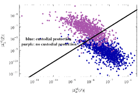
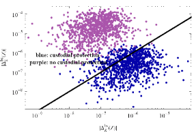
Figure 3: $|\Delta_{L}^{ij}(Z)|$ versus $|\Delta_{R}^{ij}(Z)|$ for $ij=sd$ (left) and $ij=bs$ (right). The blue points are obtained in the custodially protected model after imposing all constraints from $\Delta F=2$ observables [1]. The purple points show the effect of removing the custodial protection, as outlined in Section 7.6. The solid lines display the equality $|\Delta_{L}^{ij}(Z)|=|\Delta_{R}^{ij}(Z)|$.

As the tree level $Z$ contributions turn out to be dominant, from now on we restrict our discussion to these contributions. In Fig. 3 we show the allowed ranges for $\Delta_{L,R}^{sd}(Z)$ and $\Delta_{L,R}^{bs}(Z)$, respectively. The solid thick line corresponds to the equality of left- and right-handed couplings. We observe:

• $\Delta_{R}^{sd}(Z)$ is larger than $\Delta_{L}^{sd}(Z)$ for a dominant part of the allowed points and is on average larger than $\Delta_{L}^{sd}(Z)$ by two orders of magnitude.

• The dominance of $\Delta_{R}^{bs}(Z)$ over $\Delta_{L}^{bs}(Z)$ is less pronounced, but still on average $\Delta_{R}^{bs}(Z)$ is larger than $\Delta_{L}^{bs}(Z)$ by one order of magnitude.

• The values of $\Delta_{R}^{bs}(Z)$ are on average larger than $\Delta_{R}^{sd}(Z)$ by one order of magnitude, as the $(b_{R},s_{R})$ system is localised closer to the IR brane than the $(s_{R},d_{R})$ system.

For $\Delta_{L,R}^{bd}(Z)$ we find the values between those for the $(bs)$ and $(sd)$ cases.

When comparing the size of NP effects in $K$ and $B_{d,s}$ systems we have to take into account that NP contributions are also enhanced non-universally by factors $1/\lambda_{t}^{(i)}$. As $\lambda_{t}^{(K)}\simeq 4\cdot 10^{-4}$, whereas $\lambda_{t}^{(d)}\simeq 1\cdot 10^{-2}$ and $\lambda_{t}^{(s)}\simeq 4\cdot 10^{-2}$, we would naively expect the deviation from the SM functions in the $K$ system to be by an order of magnitude larger than in the $B_{d}$ system, and even by a larger factor than in the $B_{s}$ system. This strong hierarchy in the factors $1/\lambda_{t}^{(i)}$ is partially compensated by the opposite hierarchy in $\Delta_{R}^{ij}(Z)$. However, as flavour violation is generally weaker in the right-handed sector, this compensation is not complete, so that still larger effects are expected in $K$ physics than in $B_{d,s}$ physics. In any case the universality for the functions $X$, $Y$ and $Z$ in the $K$ and $B$ systems is necessarily broken.

Having at hand numerical results for $\Delta_{R}^{sd,bd,bs}(Z)$ for a large number of parameter sets, we can predict the average relative size of NP contributions in the $K$ and $B$ systems. We find that the size of the NP contributions on average drops by a factor of four when going from the $K$ to the $B_{d}$ system and by another factor of two when going from the $B_{d}$ to the $B_{s}$ system.

7.6 Removing the Protection of Left-Handed $Z$ Couplings

It is instructive to investigate how our results would look like if the protection of the left-handed $Z$ couplings to down-type quarks was not present. In order to get a rough idea we simply removed the contributions of the $Z^{(1)}_{X}$ gauge boson to the $Z$, $Z_{H}$ and $Z^{\prime}$ couplings that are generated in the process of electroweak symmetry breaking. This also has an impact on the right-handed $Z$ couplings, as those were dominated by the $Z_{X}^{(1)}$ contribution and are now suppressed by a factor $\sin^{2}\theta_{W}\simeq 0.2$. However the main effect is the enhancement of the couplings $\Delta_{L}^{ij}(Z)$ by roughly two orders of magnitude. The results are displayed by the purple points in Fig. 3 for the $K$ and $B_{s}$ systems. We observe that $\Delta_{L}^{sd}(Z)$ tends now to be larger than $\Delta_{R}^{sd}(Z)$, while $\Delta_{L}^{bs}(Z)$ fully dominates over $\Delta_{R}^{bs}(Z)$. Again intermediate results are found for $\Delta_{L,R}^{bd}(Z)$.

It is important to note that now, as the rare decays in question are fully dominated by the $\Delta_{L}^{ij}(Z)$ contribution, the expected pattern of deviations from the SM changes drastically with respect to the custodially protected scenario. As $\Delta_{L}^{ij}(Z)$ exhibit a similar hierarchy as the CKM factors $\lambda_{t}^{(q)}$, relative NP effects of roughly equal size are expected in $K$ and $B$ decays. We stress however that a more quantitative analysis in that case requires also the inclusion of the $Zb_{L}\bar{b}_{L}$ constraint, possibly altering the pattern of expected effects. In addition, removing the $Z_{X}^{(1)}$ couplings also modifies the predictions for $\Delta B=2$ observables at the ${\cal O}(100\%)$ level, so that the points from our parameter scan do in general not fulfil the associated constraints any more. On the other hand the most severe constraint comes from $\varepsilon_{K}$, which we have shown in [1] to be dominated by KK gluon contributions and thus insensitive to the precise structure of the EW sector. Consequently we do not expect our results to be affected significantly by this simplified working assumption.

In the next section we will show a couple of examples of how removing the protection in question influences rare decay branching ratios.

8 Numerical Analysis

8.1 Preliminaries

In our numerical analysis we will set $|V_{us}|$, $|V_{cb}|$ and $|V_{ub}|$ to their central values measured in tree level decays and collected in Table 2.

$\lambda=|V_{us}|=0.226(2)$	$G_{F}=1.16637\cdot 10^{-5}\,{\rm GeV}^{-2}$
$|V_{ub}|=3.8(4)\cdot 10^{-3}$	$M_{W}=80.403(29)\,{\rm GeV}$
$|V_{cb}|=4.1(1)\cdot 10^{-2}$ [53]	$\alpha(M_{Z})=1/127.9$
$\gamma=75(25)^{\circ}$	$\sin^{2}\theta_{W}=0.23122$
$\Delta M_{K}=0.5292(9)\cdot 10^{-2}\,\text{ps}^{-1}$	$m_{K}^{0}=497.648\,{\rm MeV}$
$|\varepsilon_{K}|=2.232(7)\cdot 10^{-3}$ [54]	$m_{B_{d}}=5279.5\,{\rm MeV}$
$\Delta M_{d}=0.507(5)\,\text{ps}^{-1}$	$m_{B_{s}}=5366.4\,{\rm MeV}$ [54]
$\Delta M_{s}=17.77(12)\,\text{ps}^{-1}$	$\eta_{1}=1.32(32)$ [55]
$S_{\psi K_{S}}=0.671(24)$ [56]	$\eta_{3}=0.47(5)$ [57, 58]
$\bar{m}_{c}=1.30(5)\,{\rm GeV}$	$\eta_{2}=0.57(1)$
$\bar{m}_{t}=162.7(13)\,{\rm GeV}$	$\eta_{B}=0.55(1)$ [59, 60]
$F_{K}=156(1)\,{\rm MeV}$ [61]	$F_{B_{s}}=245(25)\,{\rm MeV}$
$\hat{B}_{K}=0.75(7)$	$F_{B_{d}}=200(20)\,{\rm MeV}$
$\hat{B}_{B_{s}}=1.22(12)$	$F_{B_{s}}\sqrt{\hat{B}_{B_{s}}}=270(30)\,{\rm MeV}$
$\hat{B}_{B_{d}}=1.22(12)$	$F_{B_{d}}\sqrt{\hat{B}_{B_{d}}}=225(25)\,{\rm MeV}$
$\hat{B}_{B_{s}}/\hat{B}_{B_{d}}=1.00(3)$ [62]	$\xi=1.21(4)$ [62]
$\tau(B_{s})=1.470(26)\,\text{ps}$	$\alpha_{s}(M_{Z})=0.118(2)$ [54]
$\tau(B_{d})=1.530(9)\,\text{ps}$ [54]

Table 2: Values of the experimental and theoretical quantities used as input parameters.

As the fourth parameter we choose the angle $\gamma$ of the standard unitarity triangle that to an excellent approximation equals the phase $\delta_{\text{CKM}}$ in the CKM matrix. The angle $\gamma$ has been extracted from $B\to D^{(*)}K$ decays without the influence of NP. The value used throughout our analysis and quoted in Table 2 is consistent with recent fit results [53, 63].

The “true” value of $\beta$ is obtained from

$$R_{b}=\left(1-\frac{\lambda^{2}}{2}\right)\frac{1}{\lambda}\frac{|V_{ub}|}{|V_{cb}|}=0.40\pm 0.04$$ (8.1)

and $\gamma$, i. e. from tree level decays only and is not affected by a potential NP phase. We find then

$$(\sin 2\beta)_{\rm true}=(0.726\pm 0.070),\qquad\beta_{\rm true}=(23.3\pm 2.9)^{\circ}\,,$$ (8.2)

that is consistent with $S_{\psi K_{S}}$ in Table 2, although a bit larger implying a small negative value of a NP phase $\varphi_{B_{d}}$ in $B_{d}-\bar{B}_{d}$ mixing:

$$S_{\psi K_{S}}=\sin(2\beta_{\rm true}+2{\varphi_{B_{d}}}),\qquad{\varphi_{B_{d}}}=-(2.2\pm 3.1)^{\circ}\,,$$ (8.3)

as discussed already by several authors in the literature. This new phase can be easily obtained in the model considered [1].

As pointed out recently in [64], the value of $S_{\psi K_{S}}$ in Table 2 and even the value of $(\sin 2\beta)_{\rm true}$ given above appear too small to obtain the experimental value of the CP-violating parameter $\varepsilon_{K}$ in the SM. Similar tensions between CP-violation in $K^{0}-\bar{K}^{0}$ and $B_{d}^{0}-\bar{B}_{d}^{0}$ mixings from a different point of view have been pointed out in [65]. All these tensions can be removed in the model considered.

For the non-perturbative parameters entering the analysis of particle-antiparticle mixing we choose and collect in Table 2 their lattice averages given in [62].

In order to simplify our numerical analysis we will, as in [1], set all non-perturbative parameters to their central values and instead we will allow $\Delta M_{K}$, $\varepsilon_{K}$, $\Delta M_{d}$, $\Delta M_{s}$ and $S_{\psi K_{S}}$ to differ from their experimental values by $\pm 50\%$, $\pm 20\%$, $\pm 30\%$, $\pm 30\%$ and $\pm 20\%$, respectively. In the case of $\Delta M_{s}/\Delta M_{d}$ we will choose $\pm 20\%$, as the error on the relevant parameter, $\xi$, is smaller than in the case of $\Delta M_{d}$ and $\Delta M_{s}$ separately. The relevant expressions for these observables within the model considered are given in [1]. These uncertainties could appear rather conservative, but we do not want to miss any interesting effect by choosing too optimistic non-perturbative uncertainties.

In presenting the results below we impose all existing constraints from $\Delta F=2$ transitions analysed by us in [1] and require that all quark masses and weak mixing angles calculated in this model agree with the experimental ones within $2\sigma$. The details behind this latter calculation are given in [1]. Specifically we use the parameterisation of the 5D Yukawa couplings presented in that paper, where we scan over $0\leq y^{i}_{u,d}\leq 3$ in order to maintain perturbativity, and vary the relevant mixing angles and CP-violating phases in their physical ranges $[0,\pi/2]$ and $[0,2\pi]$, respectively. For the bulk mass parameters we impose $0.1\leq c_{Q}^{3}\leq 0.5$ and fit the other values in order to obtain correct quark masses and CKM mixing angles. For further details on the parameter scan we refer the reader to [1].

As there is some fine-tuning required to fit the experimental value of $\varepsilon_{K}$ we will consider as our main results for rare decays those obtained from points in the parameter space for which this fine-tuning is moderate and characterised by the Barbieri-Giudice [66] measure $\Delta_{\rm BG}(\varepsilon_{K})\leq 20$. They are given by orange points in the plots below. However, for completeness we will also show results obtained for arbitrarily high fine-tuning. They are represented by blue points in the figures below and obviously show on average larger deviations from the SM than the ones found with only moderate fine-tuning. To be specific, all the statements from now on apply only to the latter points. For some examples we also show the results obtained after removing the custodial protection. In that case points with arbitrarily high fine-tuning are shown in purple, while points with moderate fine-tuning are shown in green.

We will perform the numerical analysis in the same spirit as in the LHT model so that an easy comparison of the results obtained in the LHT model [33, 43] and the results in the model discussed here will be possible. Therefore the presentation below follows closely subsections 10.4–10.11 of [33], although it contains new correlations that cannot be found in [33].

8.2 Breakdown of Universality

In CMFV models the functions $X_{i}$, $Y_{i}$ and $Z_{i}$ are real and independent of the index $i=K,d,s$. Consequently, they are universal quantities implying strong correlations between observables in $K$, $B_{d}$ and $B_{s}$ systems. In the model discussed here this universality is generally broken, as clearly seen in the formulae of Sections 4 and 5. Moreover the functions $X_{i}$, $Y_{i}$ and $Z_{i}$ become complex quantities and their phases turn out to exhibit a non-universal behaviour.

To get a feeling for the possible sizes of $|X_{i}|$, $|Y_{i}|$ and $|Z_{i}|$ $(i=K,d,s)$ we give the 5$\sigma$ ranges for the distribution of the respective quantity. To also capture non-symmetric distributions around the mean value, for each quantity we determine the standard deviations for two symmetrised versions of the distribution: one that originates from those values only that are larger than the mean value, and the other one originating from those values only that are smaller than the mean value. Numerically we find

$$0.60\leq\frac{|X_{K}|}{X(x_{t})}\leq 1.30\,,\qquad 0.90\leq\frac{|X_{d}|}{X(x_{t})}\leq 1.12\,,\qquad 0.95\leq\frac{|X_{s}|}{X(x_{t})}\leq 1.08\,,$$ (8.4)

implying that the CP-conserving effects in the $K$ system can be much larger than in the $B_{d}$ and $B_{s}$ systems, where NP effects are found to be disappointingly small.

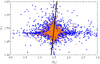
Figure 4: Breakdown of the universality between $|X_{K}|$ and $|X_{s}|$. The solid thick line represents the CMFV relation $|X_{s}|=|X_{K}|$ and the crossing point of the three solid lines indicates the SM prediction.

We illustrate this in Fig. 4, where we show the ranges allowed in the space $(|X_{K}|,|X_{s}|)$. The solid thick line represents the CMFV relation $|X_{s}|=|X_{K}|$ and the crossing point of the thin solid lines indicates the SM value. The departure from the solid thick line gives the size of non-CMFV contributions that are caused dominantly by NP effects in the $K$ system.

Similar hierarchies are found for $|Y_{i}|$ and $|Z_{i}|$:

$$0.45\leq\frac{|Y_{K}|}{Y(x_{t})}\leq 1.60\,,\qquad 0.85\leq\frac{|Y_{d}|}{Y(x_{t})}\leq 1.20\,,\qquad 0.93\leq\frac{|Y_{s}|}{Y(x_{t})}\leq 1.12\,,$$ (8.5)

$$0.35\leq\frac{|Z_{K}|}{Z(x_{t})}\leq 2.05\,,\qquad 0.80\leq\frac{|Z_{d}|}{Z(x_{t})}\leq 1.30\,,\qquad 0.90\leq\frac{|Z_{s}|}{Z(x_{t})}\leq 1.17\,.$$ (8.6)

The fact that largest effects are found in the functions $Z_{i}$ and the smallest in the functions $X_{i}$ is dominantly due to the hierarchy $X(x_{t})>Y(x_{t})>Z(x_{t})$ as

$$X(x_{t})=1.48\,,\qquad Y(x_{t})=0.94\,,\qquad Z(x_{t})=0.65\,.$$ (8.7)

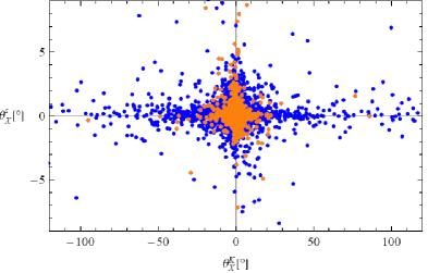
Figure 5: Breakdown of the universality between $\theta_{X}^{K}$ and $\theta_{X}^{s}$ and new sources of CP-violation. In the SM, $\theta_{X}^{K}=\theta_{X}^{s}=0$.

For the new complex phases we find the ranges

$$-45^{\circ}\leq\theta_{X}^{K}\leq 25^{\circ}\,,\qquad-9^{\circ}\leq\theta_{X}^{d}\leq 8^{\circ}\,,\qquad-2^{\circ}\leq\theta_{X}^{s}\leq 7^{\circ}\,,$$ (8.8)

implying that the new CP-violating effects in the $b\to d\nu\bar{\nu}$ and $b\to s\nu\bar{\nu}$ transitions are very small, while those in $K_{L}$ decays can be sizable. An analogous pattern is found for the phases of $Y_{i}$ and $Z_{i}$ functions:

$$-60^{\circ}\leq\theta_{Y}^{K}\leq 38^{\circ}\,,\qquad-15^{\circ}\leq\theta_{Y}^{d}\leq 12^{\circ}\,,\qquad-4^{\circ}\leq\theta_{Y}^{s}\leq 11^{\circ}\,,$$ (8.9)

$$\qquad-80^{\circ}\leq\theta_{Z}^{K}\leq 55^{\circ}\,,\qquad-21^{\circ}\leq\theta_{Z}^{d}\leq 17^{\circ}\,,\qquad-6^{\circ}\leq\theta_{Z}^{s}\leq 15^{\circ}\,.$$ (8.10)

Again the largest effects are found in the $Z_{i}$ functions. As an example we show in Fig. 5 the allowed range in the space $(\theta_{X}^{K},\theta_{X}^{s})$.

From these results it is evident that flavour universality can be significantly violated. The anatomy of the hierarchies in the factors $1/\lambda_{t}^{(i)}$ and in the gauge couplings of $Z$ leading to this breakdown and to its particular pattern can be found in Section 7.

8.3 The $K\to\pi\nu\bar{\nu}$ System

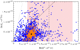
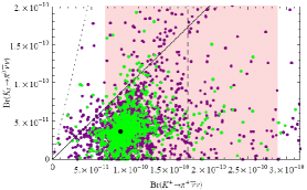
Figure 6: Left: $Br(K_{L}\rightarrow\pi^{0}\nu\bar{\nu})$ as a function of $Br(K^{+}\rightarrow\pi^{+}\nu\bar{\nu})$. The shaded area represents the experimental $1\sigma$-range for $Br(K^{+}\rightarrow\pi^{+}\nu\bar{\nu})$. The GN-bound is displayed by the dotted line, while the solid line separates the two areas where $Br(K_{L}\rightarrow\pi^{0}\nu\bar{\nu})$ is larger or smaller than $Br(K^{+}\rightarrow\pi^{+}\nu\bar{\nu})$. The black point represents the SM prediction. Right: The same, but in the case of removed custodial protection.

In the left panel of Fig. 6 we show the correlation between $Br(K^{+}\rightarrow\pi^{+}\nu\bar{\nu})$ and $Br(K_{L}\rightarrow\pi^{0}\nu\bar{\nu})$. The experimental $1\sigma$-range for $Br(K^{+}\rightarrow\pi^{+}\nu\bar{\nu})$ [67] and the model-independent Grossman-Nir (GN) bound [68] are also shown. We observe that $Br(K_{L}\rightarrow\pi^{0}\nu\bar{\nu})$ can be as large as $15\cdot 10^{-11}$, that is by a factor of 5 larger than its SM value $(2.8\pm 0.6)\cdot 10^{-11}$ while being still consistent with the measured value for $Br(K^{+}\rightarrow\pi^{+}\nu\bar{\nu})$. The latter branching ratio can be enhanced by at most a factor of 2 but this is sufficient to reach the central experimental value [67]

$$Br(K^{+}\rightarrow\pi^{+}\nu\bar{\nu})_{\text{exp}}=(17.3^{+11.5}_{-10.5})\cdot 10^{-11}\,,$$ (8.11)

to be compared with the SM value [69]

$$Br(K^{+}\rightarrow\pi^{+}\nu\bar{\nu})_{\text{SM}}=(8.5\pm 0.7)\cdot 10^{-11}\,.$$ (8.12)

In the right panel of Fig. 6 we show the modification when the custodial protection for $Z$ couplings is removed as discussed in Section 7.6. Now the values of $Br(K_{L}\rightarrow\pi^{0}\nu\bar{\nu})$ and $Br(K^{+}\rightarrow\pi^{+}\nu\bar{\nu})$ can be as large as $2\cdot 10^{-10}$ and $3\cdot 10^{-10}$ respectively, i. e. in the absence of protection an additional enhancement by almost a factor 2 is possible.

8.4 $S_{\psi\phi}$ and $K\to\pi\nu\bar{\nu}$

In our previous paper [1] spectacular NP effects in the CP-asymmetries $S_{\psi\phi}$ and $A^{s}_{\rm SL}$ have been found. Therefore let us now have a closer look at the correlations between $S_{\psi\phi}$ and the $K\to\pi\nu\bar{\nu}$ decays. In Figs. 7 and 8 we show the correlation between $S_{\psi\phi}$ and $Br(K_{L}\rightarrow\pi^{0}\nu\bar{\nu})$ and $Br(K^{+}\rightarrow\pi^{+}\nu\bar{\nu})$, respectively. We observe that it is very difficult to obtain simultaneously large deviations from the SM in the $K\to\pi\nu\bar{\nu}$ decays and in $S_{\psi\phi}$.

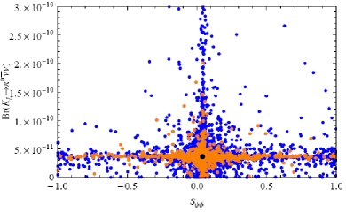
Figure 7: $Br(K_{L}\to\pi^{0}\nu\bar{\nu})$ as a function of $S_{\psi\phi}$. The black point represents the SM prediction.

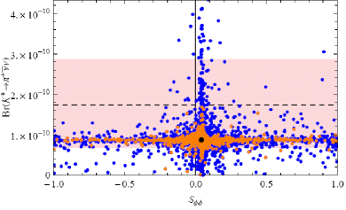
Figure 8: $Br(K^{+}\to\pi^{+}\nu\bar{\nu})$ as a function of $S_{\psi\phi}$. The shaded area represents the experimental $1\sigma$-range for $Br(K^{+}\rightarrow\pi^{+}\nu\bar{\nu})$, and the black point the SM prediction.

8.5 $B\to K\nu\bar{\nu}$, $B\to K^{*}\nu\bar{\nu}$ and $B\to X_{s,d}\nu\bar{\nu}$

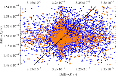
Figure 9: Correlation between $Br(B\to X_{s}\nu\bar{\nu})$ and $Br(B\to X_{d}\nu\bar{\nu})$. The black line represents the universal CMFV result given by the ratio $|V_{td}|^{2}/|V_{ts}|^{2}$, and the black point the SM prediction.

Using the formulae of Sections 4 and 5 we find the ranges

$$0.90\leq R_{1}=\frac{Br(B^{+}\to K^{+}\nu\bar{\nu})}{Br(B^{+}\to K^{+}\nu\bar{\nu})_{\rm SM}}\leq 1.15\,,\qquad 0.90\leq R_{2}\leq 1.10\,,$$ (8.13)

$$0.95\leq\frac{Br(B\to X_{s}\nu\bar{\nu})}{Br(B\to X_{s}\nu\bar{\nu})_{\rm SM}}\leq 1.08\,,$$ (8.14)

and

$$0.93\leq P\leq 1.07\,.$$ (8.15)

These results show that NP effects in rare $B$ decays are significantly smaller than in rare $K$ decays as already expected from our anatomy of NP effects in Sections 7 and 8.2. As the deviation of $P$ from unity signals violation of an important and very clean correlation between $Br(B\to X_{s}\nu\bar{\nu})$ and $Br(B\to X_{d}\nu\bar{\nu})$ in the CMFV models we show this correlation in Fig. 9. Unfortunately, the resulting deviation is small and will be difficult to measure. Therefore we do not show the correlation in (5.6) that would display strong deviations from CMFV mainly due to large effects in $K_{L}\rightarrow\pi^{0}\nu\bar{\nu}$ but small ones in $B\to X_{s}\nu\bar{\nu}$. Similar effects have already been seen in several plots in our paper in the case of other correlations between $K$ and $B$ decays.

8.6 $B_{s}\to\mu^{+}\mu^{-}$ versus $K^{+}\to\pi^{+}\nu\bar{\nu}$

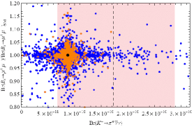
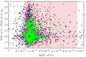
Figure 10: Left: $Br(B_{s}\to\mu^{+}\mu^{-})/Br(B_{s}\to\mu^{+}\mu^{-})_{\text{SM}}$ as a function of $Br(K^{+}\rightarrow\pi^{+}\nu\bar{\nu})$. The shaded area represents the experimental $1\sigma$-range for $Br(K^{+}\rightarrow\pi^{+}\nu\bar{\nu})$ and the black point shows the SM prediction. Right: The same, but in the case of removed custodial protection.

We next investigate the possible correlation between $B_{s}\to\mu^{+}\mu^{-}$ and $K^{+}\to\pi^{+}\nu\bar{\nu}$. To this end we show in the left panel of Fig. 10 the correlation between $Br(B_{s}\to\mu^{+}\mu^{-})/Br(B_{s}\to\mu^{+}\mu^{-})_{\text{SM}}$ and $Br(K^{+}\rightarrow\pi^{+}\nu\bar{\nu})$. The experimental $1\sigma$-range for $Br(K^{+}\rightarrow\pi^{+}\nu\bar{\nu})$ [67] is represented by the shaded area and the SM prediction by the black point. $Br(B_{s}\to\mu^{+}\mu^{-})$ can deviate only by $15\%$ from the SM value, while more pronounced effects are possible in $Br(K^{+}\rightarrow\pi^{+}\nu\bar{\nu})$ as we have seen before. Again, when $Br(K^{+}\rightarrow\pi^{+}\nu\bar{\nu})$ is sizably enhanced, $Br(B_{s}\to\mu^{+}\mu^{-})$ can hardly be distinguished from the SM prediction.

The situation changes spectacularly when the protection of $Z$ couplings is removed, as shown in the right panel of Fig. 10. While $Br(K^{+}\rightarrow\pi^{+}\nu\bar{\nu})$ can now be enhanced by another factor of two, a much bigger effect is seen in the case of $Br(B_{s}\rightarrow\mu^{+}\mu^{-})$. More precisely, the possible effects are now roughly of equal size in both decays, with even slightly bigger effects observed in $B_{s}\to\mu^{+}\mu^{-}$. This pattern can be easily understood from the discussion in Section 7.6: In the absence of custodial protection the NP effects are clearly dominated by $\Delta_{L}^{ij}(Z)$ which exhibits a similar hierarchy as the relevant CKM factors $\lambda_{t}^{(q)}$. The slightly bigger effects in $B_{s}\to\mu^{+}\mu^{-}$ are then a remnant of the hierarchy $X(x_{t})>Y(x_{t})$ in the SM, implying that NP effects are generally more pronounced in the latter case. We would like to note however that such large enhancements in $B_{s}\to\mu^{+}\mu^{-}$ are generally expected to coincide with a violation of the $Zb_{L}\bar{b}_{L}$ constraint, so that a more thorough analysis including also this latter constraint is required to make a definite prediction in the model without custodial protection.

8.7 Correlation between $K_{L}\to\mu^{+}\mu^{-}$ and $B_{s}\to\mu^{+}\mu^{-}$

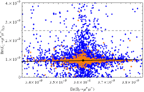
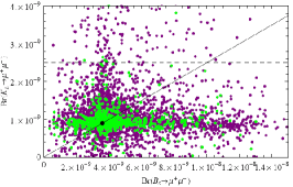
Figure 11: left: $Br(K_{L}\to\mu^{+}\mu^{-})_{\text{SD}}$ as a function of $Br(B_{s}\to\mu^{+}\mu^{-})$. The dashed line indicates the upper bound on $Br(K_{L}\to\mu^{+}\mu^{-})_{\text{SD}}$. The solid line shows the CMFV prediction, while the black point represents the SM. right: The same, but in the case of removed custodial protection.

In the left panel of Fig. 11 we show the correlation between the branching ratios for $K_{L}\to\mu^{+}\mu^{-}$ and $B_{s}\to\mu^{+}\mu^{-}$. As expected from our anatomy of NP effects, the CMFV correlation represented by the solid line is strongly broken, mainly due to much larger NP effects in the decay of $K_{L}$. We also observe that the upper bound of (4.15) can be saturated, but this happens only for SM-like values of $Br(B_{s}\to\mu^{+}\mu^{-})$.

In the right panel of Fig. 11 we show the same correlation in the absence of custodial protection for the $Z$ couplings to left-handed down-type quarks. The NP effects are now significantly larger, in particular in $B_{s}\to\mu^{+}\mu^{-}$, as already observed previously. Also in $K_{L}\to\mu^{+}\mu^{-}$ an additional enhancement by a factor of two is possible, so that the bound of (4.15) can be strongly violated. Interestingly, while the possible effects in $K_{L}\to\mu^{+}\mu^{-}$ and $B_{s}\to\mu^{+}\mu^{-}$ are now very similar, they are generally not expected to appear simultaneously, so that a strong violation of the CMFV prediction displayed by the solid line is possible.

8.8 Correlation between $K_{L}\to\mu^{+}\mu^{-}$ and $K^{+}\rightarrow\pi^{+}\nu\bar{\nu}$

Figure 12: Correlation between $K_{L}\to\mu^{+}\mu^{-}$ and $K^{+}\rightarrow\pi^{+}\nu\bar{\nu}$. The black point represents the SM prediction.

Next in Fig. 12 we show the correlation between the short distance contribution to $Br(K_{L}\to\mu^{+}\mu^{-})$ and $Br(K^{+}\rightarrow\pi^{+}\nu\bar{\nu})$. As both are CP-conserving rare $K$ decays, a non-trivial correlation is generally expected. Interestingly it turns out that this correlation is an inverse one, i. e. an enhancement of $Br(K_{L}\to\mu^{+}\mu^{-})$ relative to the SM coincides with a suppression of $Br(K^{+}\rightarrow\pi^{+}\nu\bar{\nu})$ and vice versa. This correlation originates in the fact that the $K^{+}\to\pi^{+}\nu\bar{\nu}$ transition is sensitive to the vector component of the flavour violating $Z$ coupling, while the $K_{L}\to\mu^{+}\mu^{-}$ decay measures its axial component. As the SM flavour changing $Z$ penguin is purely left-handed, while the NP contribution is dominated by right-handed $Z$ couplings, these two contributions enter the decays in question with opposite relative sign. In other words, the correlation between $K^{+}\to\pi^{+}\nu\bar{\nu}$ and $K_{L}\to\mu^{+}\mu^{-}$ offers a clear test of the handedness of NP flavour violating interactions.

8.9 The $K_{L}\to\pi^{0}\ell^{+}\ell^{-}$ System

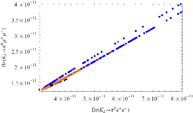
Figure 13: $Br(K_{L}\to\pi^{0}\mu^{+}\mu^{-})$ as a function of $Br(K_{L}\to\pi^{0}e^{+}e^{-})$, assuming constructive interference. The black point represents the SM prediction.

In Fig. 13 we show the correlation between $Br(K_{L}\to\pi^{0}e^{+}e^{-})$ and $Br(K_{L}\to\pi^{0}\mu^{+}\mu^{-})$ that has first been investigated in [45, 46, 47]. We observe that both branching ratios can be enhanced at most by $60\%$ over the SM values [47]

$$Br(K_{L}\to\pi^{0}e^{+}e^{-})_{\text{SM}}=3.54^{+0.98}_{-0.85}\left(1.56^{+0.62}_{-0.49}\right)\cdot 10^{-11}\,,$$ (8.16)

$$Br(K_{L}\to\pi^{0}\mu^{+}\mu^{-})_{\text{SM}}=1.41^{+0.28}_{-0.26}\left(0.95^{+0.22}_{-0.21}\right)\cdot 10^{-11}\,,$$ (8.17)

with the values in parentheses corresponding to the destructive interference between directly and indirectly CP-violating contributions. A recent discussion of the theoretical status of this interference sign can be found in [70] where the results of [45, 46, 71] are critically analysed. From this discussion, constructive interference seems to be favoured though more work is necessary. In Fig. 13 constructive interference has been assumed. We also observe a strong correlation between $Br(K_{L}\to\pi^{0}e^{+}e^{-})$ and $Br(K_{L}\to\pi^{0}\mu^{+}\mu^{-})$, similar to the case of the LHT model. Indeed such a correlation is common to all models with no scalar operators contributing to the decays in question [45, 46, 47].

The present experimental bounds

$$Br(K_{L}\to\pi^{0}e^{+}e^{-})_{\text{exp}}<28\cdot 10^{-11}\quad\text{\cite[cite]{[\@@bibref{}{AlaviHarati:2003mr}{}{}]}}\,,\qquad Br(K_{L}\to\pi^{0}\mu^{+}\mu^{-})_{\text{exp}}<38\cdot 10^{-11}\quad\text{\cite[cite]{[\@@bibref{}{AlaviHarati:2000hs}{}{}]}}\,,$$ (8.18)

are still by one order of magnitude larger than the SM predictions.

8.10 $K_{L}\to\pi^{0}\ell^{+}\ell^{-}$ versus $K_{L}\rightarrow\pi^{0}\nu\bar{\nu}$

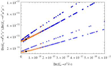
Figure 14: $Br(K_{L}\to\pi^{0}e^{+}e^{-})$ (upper curve) and $Br(K_{L}\to\pi^{0}\mu^{+}\mu^{-})$ (lower curve) as functions of $Br(K_{L}\rightarrow\pi^{0}\nu\bar{\nu})$. The corresponding SM predictions are represented by black points.

In Fig. 14 we show $Br(K_{L}\to\pi^{0}e^{+}e^{-})$ and $Br(K_{L}\to\pi^{0}\mu^{+}\mu^{-})$ versus $Br(K_{L}\rightarrow\pi^{0}\nu\bar{\nu})$. We observe a strong correlation between the $K_{L}\to\pi^{0}\ell^{+}\ell^{-}$ and $K_{L}\rightarrow\pi^{0}\nu\bar{\nu}$ decays that has already been found in the LHT model [33]. We note that a large enhancement of $Br(K_{L}\rightarrow\pi^{0}\nu\bar{\nu})$ automatically implies significant enhancements of $Br(K_{L}\to\pi^{0}\ell^{+}\ell^{-})$, although the NP effects in $K_{L}\rightarrow\pi^{0}\nu\bar{\nu}$ are much stronger. This is related to the fact that NP effects in $K_{L}\to\pi^{0}\ell^{+}\ell^{-}$ are shadowed by the dominant indirectly CP-violating contribution. The correlations in Figs.  13 and 14 constitute a powerful test of the model considered. Again the correlation observed here is very similar to the one encountered in the LHT model [33].

8.11 Violation of Golden MFV Relations

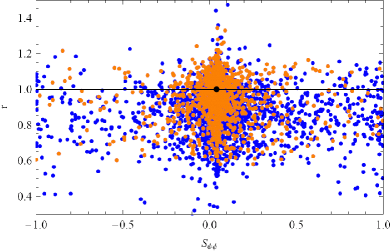
Figure 15: The ratio $r$ of (8.19) as a function of $S_{\psi\phi}$. The solid line indicates the CMFV prediction and the black point the SM value.

There are two golden relations that are theoretically very clean and consequently are very suitable for the tests of the SM and its extentions.

We have first the relation between $Br(B_{d,s}\to\mu^{+}\mu^{-})$ and $\Delta M_{d}/\Delta M_{s}$ valid in CMFV models [51] that in the model in question and also in the LHT model gets modified as follows:

$$\frac{Br(B_{s}\to\mu^{+}\mu^{-})}{Br(B_{d}\to\mu^{+}\mu^{-})}=\frac{\hat{B}_{B_{d}}}{\hat{B}_{B_{s}}}\frac{\tau(B_{s})}{\tau(B_{d})}\frac{\Delta M_{s}}{\Delta M_{d}}\,r\,,\quad r=\left|\frac{Y_{s}}{Y_{d}}\right|^{2}\frac{C_{B_{d}}}{C_{B_{s}}}\,,\qquad{C_{B_{d,s}}=\frac{\Delta M_{d,s}}{(\Delta M_{d,s})_{\text{SM}}}\,,}$$ (8.19)

with $r=1$ in CMFV models but generally different from unity.

In Fig. 15 we show the ratio $r$ of (8.19) as a function of $S_{\psi\phi}$. The departure from unity measures the violation of the golden CMFV relation between $B_{d,s}\to\mu^{+}\mu^{-}$ decays and $\Delta M_{d,s}$ in (8.19). We observe that $r$ can vary roughly in the range

$${0.60}\leq r\leq 1.35\,,$$ (8.20)

with only a weak correlation with $S_{\psi\phi}$.

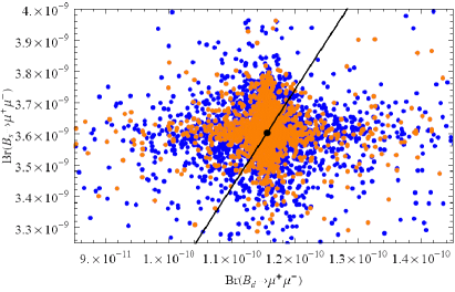
Figure 16: $Br(B_{s}\to\mu^{+}\mu^{-})$ versus $Br(B_{d}\to\mu^{+}\mu^{-})$. The straight line represents the CMFV correlation and the black point the SM prediction.

It is instructive to show also the plot of $Br(B_{s}\to\mu^{+}\mu^{-})$ versus $Br(B_{d}\to\mu^{+}\mu^{-})$ that in CMFV models is a straight line with the slope given in (8.19) with $r=1$. A similar strong correlation within general MFV models exists [74]. As shown in Fig. 16 deviations from this straight line signal non-CMFV effects present in the model considered. We note that NP effects in $B_{d}\to\mu^{+}\mu^{-}$ are larger than in $B_{s}\to\mu^{+}\mu^{-}$ as expected from our discussion in Section 8.2, but in any case both are small and difficult to be tested in future experiments.

Another golden test of the MFV hypothesis is given by the ratio

$$\frac{\sin{2\beta_{X}^{K}}}{\sin{2(\beta+\varphi_{B_{d}})}}\,,$$ (8.21)

i. e. by comparing CP-violation in $B_{d}-\bar{B}_{d}$ mixing and the decay $K_{L}\rightarrow\pi^{0}\nu\bar{\nu}$. While in models with new flavour and CP-violating interactions, such as the LHT model [33, 43], this ratio can deviate significantly from unity, in MFV models $\varphi_{B_{d}}=0,\,\theta^{K}_{X}=0$ holds, so that the MFV relation of [50, 49]

$$(\sin 2\beta)_{S_{\psi K_{S}}}=(\sin 2\beta)_{K_{L}\rightarrow\pi^{0}\nu\bar{\nu}}$$ (8.22)

is recovered and the ratio in (8.21) is very close to 1. A violation of this relation would thus clearly signal the presence of new complex phases and non-MFV interactions.

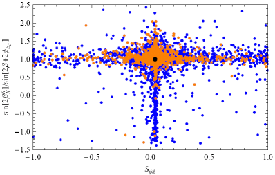
Figure 17: $\sin 2\beta_{X}^{K}/\sin(2\beta+2\varphi_{B_{d}})$ as a function of $S_{\psi\phi}$. The departure from unity (solid line) measures the size of non-MFV effects. The black point represents the SM prediction.

In Fig. 17 we show the ratio of $\sin 2\beta_{X}^{K}$ over $\sin(2\beta+2\varphi_{B_{d}})$ as a function of $S_{\psi\phi}$. As discussed in Section 8.1, $\varphi_{B_{d}}$ is found to be small, and large violations of the relation in question can only follow from large deviations of $X_{K}$ from its SM value. As seen in Fig. 17, they can be significant, but again only for SM-like values of $S_{\psi\phi}$.

8.12 Comparison with the Results in the LHT Model

The pattern of deviations from the SM predictions found in the RS model analysed here and in [1] differs from the one found in the LHT model [75, 33, 43]:

• NP effects in $S_{\psi\phi}$ analysed already in [1] can be large in both models but the ones in the RS model can generally be larger due to the larger number of free flavour parameters and to the presence of the $\mathcal{Q}_{LR}$ operators that are absent in the LHT model.

• NP effects in rare $K$ decays can be large in both models but this time it is easier to enhance the relevant branching ratios in the LHT model, in particular in the case of CP-conserving decays like $K^{+}\to\pi^{+}\nu\bar{\nu}$. Even if FCNC transitions take place in the RS model already at the tree level, the custodial protection of left-handed $Z$ couplings, the RS-GIM mechanism and masses of the gauge bosons in this model larger ($(2-3)$ TeV) than the masses of new electroweak gauge bosons in the LHT model (typically smaller than 1 TeV) taken together do not allow for effects as large as the one-loop effects in the LHT model.

• The correlations between $K_{L}\to\pi^{0}\mu^{+}\mu^{-}$ and $K_{L}\to\pi^{0}e^{+}e^{-}$ and between $K_{L}\to\pi^{0}\ell^{+}\ell^{-}$ and $K_{L}\rightarrow\pi^{0}\nu\bar{\nu}$ decays are similar in the RS model considered and in the LHT model.

• The situation is different for the $K\to\pi\nu\bar{\nu}$ system, where in the LHT model a strong correlation between $K_{L}\rightarrow\pi^{0}\nu\bar{\nu}$ and $K^{+}\to\pi^{+}\nu\bar{\nu}$ has been found [33, 43]. This should be contrasted to the case of the RS model, where we observe no visible correlation between these two decays.

• A similar pattern of NP effects is observed in rare $B$ decays but the effects are generally smaller than in $K$ decays in both models.

• A drastically different situation is encountered in the RS model without custodial protection, where the possible NP effects in rare $K$ and $B$ decays are expected to be of equal size. In particular $Br(B_{s}\to\mu^{+}\mu^{-})$ can be enhanced by as much as a factor of three which is clearly impossible in the LHT model. However, as already stated, our analysis is not complete, since in this scenario also a strong violation of the $Zb_{L}\bar{b}_{L}$ constraint is generally predicted and a consistent analysis should take into account also EW precision observables.

• In both models it is unlikely to obtain simultaneously large effects in $S_{\psi\phi}$ and in rare $K$ decays, but in the RS model considered here this effect is more pronounced.

In summary, despite the completely different sources of flavour violation in the RS model and in the LHT model, the general pattern of flavour violating observables is similar in both models and makes a distinction non-trivial. Still some signatures would clearly favour one or the other model. In particular:

• An observation of the CP-asymmetry $S_{\psi\phi}$ larger than about 0.4 would strongly disfavour the LHT model and favour RS physics.

• Another clear falsification of the LHT model could be offered by finding the $K\to\pi\nu\bar{\nu}$ decay rates outside the correlation predicted by the LHT model.

• On the other hand, the observation of simultaneous large NP effects in $S_{\psi\phi}$ and in rare $K$ decays would put the RS model under severe pressure.

9 Summary and Outlook

In the present paper we have performed a detailed analysis of the most interesting rare decays of $K$ and $B$ mesons in a warped extra dimensional model with a custodial protection of flavour diagonal and flavour non-diagonal $Z$ boson couplings to left-handed down-type quarks. In this model NP contributions come dominantly from tree level exchanges of $Z$ bosons governed by its couplings to right-handed down-type quarks. The contributions of the $Z_{H}$ boson are significantly smaller, while those from $Z^{\prime}$ are negligible, being suppressed by the custodial protection mechanism, its large mass and small couplings to leptons. Also the contributions of the KK photon $A^{(1)}$ are negligible, being suppressed by the small electromagnetic coupling constant and by the electric charge of the down-type quarks. The anatomy of various contributions has been presented in Section 7.

Using the Feynman rules of [18] we have calculated the short distance functions $X_{i}$, $Y_{i}$ and $Z_{i}$ ($i=K,d,s$). In the model in question these functions are complex quantities and carry the index $i$ to signal the breakdown of the universality of FCNC processes, valid in the SM and MFV models. The new weak phases in $X_{i}$, $Y_{i}$ and $Z_{i}$, which are absent in the SM and models with MFV, imply potential new CP-violating effects beyond the SM and MFV ones.

With the functions $X_{i}$, $Y_{i}$ and $Z_{i}$ at hand, we have calculated the branching ratios for a number of interesting rare decays. In particular, we analysed $K^{+}\to\pi^{+}\nu\bar{\nu}$, $K_{L}\to\pi^{0}\nu\bar{\nu}$, $K_{L}\to\pi^{0}\ell^{+}\ell^{-}$, $K_{L}\to\mu^{+}\mu^{-}$, $B_{s,d}\to\mu^{+}\mu^{-}$, $B\to K\nu\bar{\nu}$, $B\to K^{*}\nu\bar{\nu}$ and $B\to X_{s,d}\nu\bar{\nu}$. At all stages of our numerical analysis we took into account the existing constraints from $\Delta F=2$ processes analysed by us in [1].

The main messages of our paper are as follows:

• The most evident departures from the SM predictions are found for CP-violating observables that are strongly suppressed within the SM. These are the branching ratio for $K_{L}\to\pi^{0}\nu\bar{\nu}$ and the CP-asymmetry $S_{\psi\phi}$ with the latter analysed already in [1]. $Br\left(K_{L}\rightarrow\pi^{0}\nu\bar{\nu}\right)$ can be by a factor of 5 larger than its SM value, while $S_{\psi\phi}$ can be enhanced by more than an order of magnitude. However as clearly seen in Fig. 7 simultaneous large NP effects in both observables are very unlikely.

• The largest departures from SM expectations for $Br\left(K^{+}\rightarrow\pi^{+}\nu\bar{\nu}\right)$ and $Br(K_{L}\to\pi^{0}\ell^{+}\ell^{-})$ amount to factors of $2$ and $1.6$, respectively. The enhancement of $Br(K^{+}\rightarrow\pi^{+}\nu\bar{\nu})$ could be welcomed one day if the central experimental value will remain in the ballpark of $15\cdot 10^{-11}$ and its error will decrease. Again, it is very unlikely to get simultaneously large NP effects in $K^{+}\rightarrow\pi^{+}\nu\bar{\nu}$ and $S_{\psi\phi}$ (Fig. 8), while simultaneous large effects in $K^{+}\rightarrow\pi^{+}\nu\bar{\nu}$ and $K_{L}\rightarrow\pi^{0}\nu\bar{\nu}$ are possible as clearly seen in Fig. 6.

• The branching ratios for $B_{s,d}\to\mu^{+}\mu^{-}$ and $B\to X_{s,d}\nu\bar{\nu}$, instead, are modified by at most $20\%$ and $10\%$, respectively.

• Sizable departures from MFV relations between $\Delta M_{s,d}$ and $Br(B_{s,d}\to\mu^{+}\mu^{-})$ and between $S_{\psi K_{S}}$ and the $K\to\pi\nu\bar{\nu}$ decay rates are possible. This is clearly seen in Figs. 15 and 17.

• The universality of NP effects, characteristic for MFV models, can be largely broken, in particular between $K$ and $B_{s,d}$ systems in $\Delta F=1$ transitions, where large effects are only possible in $K$ decays.

• The main impact of the extended gauge group on $\Delta F=1$ processes is the suppression of tree level left-handed $Z$ couplings, while the direct contributions of the new gauge bosons play a subdominant role.

In summary, our present analysis of rare $K$ and $B$ decays combined with our previous analysis of $\Delta F=2$ transitions reveals a clear pattern of NP effects in FCNC processes predicted by the RS model with custodial protection in question:

• NP effects in $\Delta S=2$ processes are governed by KK gluons, whereas in $\Delta B=2$ transitions the heavy gauge boson $Z_{H}$ is equally important.

• NP effects in $\Delta S=1$ transitions are dominated by tree level $Z$ exchanges.

• Large effects in $S_{\psi\phi}$ are possible.

• Large effects in $K_{L}\rightarrow\pi^{0}\nu\bar{\nu}$ and $K^{+}\rightarrow\pi^{+}\nu\bar{\nu}$ are possible, even simultaneously.

• Large enhancements in $K_{L}\to\mu^{+}\mu^{-}$ and $K^{+}\rightarrow\pi^{+}\nu\bar{\nu}$ are possible, but not simultaneously.

• Simultaneous large effects in $S_{\psi\phi}$ and in the $K\to\pi\nu\bar{\nu}$ decays are very unlikely.

• NP effects in rare $B$ decays dominated in the SM by $Z$ penguin contributions are generally small and hardly distinguishable from NP effects in MFV models.

This pattern implies that an observation of a large $S_{\psi\phi}$ would in the context of the model considered here preclude sizable NP effects in rare $K$ decays. On the other hand, finding $S_{\psi\phi}$ to be SM-like will open the road to large NP effects in rare $K$ decays. Independently of the experimental value of $S_{\psi\phi}$, NP effects in rare $B$ decays are predicted to be small and an observation of large departures from SM predictions in future data would put the model considered here in serious difficulties.

Clearly, this pattern of NP effects in FCNC processes originates to a large extent in the custodial protection of the $Z$ couplings to left-handed down-type quarks. We have shown that removing this protection from the model allows to obtain significantly larger NP effects in rare $K$ and $B$ decays. For instance $Br(B_{s}\to\mu^{+}\mu^{-})$ could be as large as $10^{-8}$. On the other hand without this protection it is much harder to obtain an agreement with the electroweak precision data for KK scales in the reach of the LHC.

Finally, as a byproduct we have presented general formulae for effective Hamiltonians including right-handed couplings to gauge bosons that can be used in any extension of the SM. We have also pointed out a number of correlations between various decays (see Section 6) that could turn out to be crucial for distinguishing various NP scenarios.

Acknowledgments

We thank Csaba Csaki and Andreas Weiler for useful discussions. This research was partially supported by the Graduiertenkolleg GRK 1054, the Deutsche Forschungsgemeinschaft (DFG) under contract BU 706/2-1, the DFG Cluster of Excellence ‘Origin and Structure of the Universe’ and by the German Bundesministerium für Bildung und Forschung under contract 05HT6WOA. S. G. acknowledges support by the European Community’s Marie Curie Research Training Network under contract MRTN-CT-2006-035505 [“HEPTOOLS”].

Appendix A Couplings of Electroweak Gauge Bosons

A.1 Couplings of $Z$

The flavour non-diagonal couplings of $Z$ to down quarks are given by

$$\Delta_{L,R}^{ij}(Z)=\frac{M_{Z}^{2}}{M_{\text{KK}}^{2}}\left[-\mathcal{I}^{+}_{1}\Delta_{L,R}^{ij}(Z^{(1)})+\mathcal{I}^{-}_{1}\cos\phi\,\cos\psi\Delta_{L,R}^{ij}(Z^{(1)}_{X})\right]{+\Delta_{L,R}^{ij}(Z)_{\text{KK-fermions}}\,,}$$ (A.1)

where

$$\mathcal{I}_{1}^{+} = \frac{1}{L}\int_{0}^{L}dy\,e^{-2ky}g(y)h(y)^{2}{\simeq\sqrt{2kL}}\,,$$ (A.2)

$$\mathcal{I}_{1}^{-} = \frac{1}{L}\int_{0}^{L}dy\,e^{-2ky}\tilde{g}(y)h(y)^{2}{\simeq\sqrt{2kL}}\,.$$ (A.3)

Here $h(y)$ is the Higgs profile, with $h(y)\propto\delta(y-L)$ in the present analysis, and $g(y),\tilde{g}(y)$ are the shape functions of $Z^{(1)}$ and $Z_{X}^{(1)}$, respectively, differing slightly from each other due to the different boundary conditions on the UV brane. $Z^{(1)}$ and $Z^{(1)}_{X}$ are gauge eigenstates and $\Delta_{L,R}^{ij}(Z^{(1)})$ and $\Delta_{L,R}^{ij}(Z^{(1)}_{X})$ are the elements of the $3\times 3$ coupling matrices

$$\hat{\Delta}_{L,R}(V)=\mathcal{D}_{L,R}^{\dagger}\hat{\varepsilon}_{L,R}(V)\mathcal{D}_{L,R}\qquad(V=Z^{(1)},Z_{X}^{(1)})\,,$$ (A.4)

with $\mathcal{D}_{L}$ and $\mathcal{D}_{R}$ being the left- and right-handed down-type flavour mixing matrices, respectively. They have been discussed and calculated in [1]. $\hat{\varepsilon}_{L,R}(Z^{(1)})$ and $\hat{\varepsilon}_{L,R}(Z_{X}^{(1)})$ are diagonal matrices

$$\hat{\varepsilon}_{L,R}(V)=\text{diag}\big{(}\varepsilon_{L,R}(1)(V),\varepsilon_{L,R}(2)(V),\varepsilon_{L,R}(3)(V)\big{)}\qquad(V=Z^{(1)},Z_{X}^{(1)})\,.$$ (A.5)

The couplings of $Z^{(1)}$ and $Z_{X}^{(1)}$ to fermions in the flavour eigenbasis are given by the overlap integrals

$$\varepsilon_{L}(i)(Z^{(1)}) = g_{Z,L}^{\text{4D}}\frac{1}{L}\int_{0}^{L}dy\,e^{ky}\left[f^{(0)}_{L}(y,c_{Q}^{i})\right]^{2}g(y)\,,$$ (A.6)

$$\varepsilon_{R}(i)(Z^{(1)}) = g_{Z,R}^{\text{4D}}\frac{1}{L}\int_{0}^{L}dy\,e^{ky}\left[f^{(0)}_{R}(y,c_{d}^{i})\right]^{2}g(y)\,,$$ (A.7)

$$\varepsilon_{L}(i)(Z_{X}^{(1)}) = \kappa_{1}^{\text{4D}}\frac{1}{L}\int_{0}^{L}dy\,e^{ky}\left[f^{(0)}_{L}(y,c_{Q}^{i})\right]^{2}\tilde{g}(y)\,,$$ (A.8)

$$\varepsilon_{R}(i)(Z_{X}^{(1)}) = \kappa_{5}^{\text{4D}}\frac{1}{L}\int_{0}^{L}dy\,e^{ky}\left[f^{(0)}_{R}(y,c_{d}^{i})\right]^{2}\tilde{g}(y)\,.$$ (A.9)

Further

$$g_{Z,L}^{\text{4D}}=\frac{g^{\text{4D}}}{\cos\psi}\left(-\frac{1}{2}+\frac{1}{3}\sin^{2}\psi\right)\, ~{}~{}~{}~{}\kappa_{1}^{\text{4D}}=\frac{g^{\text{4D}}}{\cos\phi}\left(-\frac{1}{2}-\frac{1}{6}\sin^{2}\phi\right)\,,$$ , (A.10)

$$g_{Z,R}^{\text{4D}}=\frac{g^{\text{4D}}}{\cos\psi}\left(\frac{1}{3}\sin^{2}\psi\right)\, ~{}~{}~{}~{}\kappa_{5}^{\text{4D}}=\frac{g^{\text{4D}}}{\cos\phi}\left(-1+\frac{1}{3}\sin^{2}\phi\right)\,.$$ , (A.11)

Here $g^{\text{4D}}$ is the 4D $SU(2)_{L}$ gauge coupling. Moreover $\sin^{2}\psi\approx\sin^{2}\theta_{W}$ and $\sin\phi$, $\cos\phi$ as functions of $\psi$ are given by the formulae

$$\cos\psi=\frac{1}{\sqrt{1+\sin^{2}\phi}}\,,\qquad\sin\psi=\frac{\sin\phi}{\sqrt{1+\sin^{2}\phi}}$$ (A.12)

and can also be found in [18].

Finally, the contribution to the flavour violating $Z$ couplings originating from the mixing of the fermionic zero modes with their heavy KK partners turns out to be a sub-leading effect [1]. The corresponding formulae are complicated and beyond the scope of this paper. Details will be presented elsewhere. Note that both gauge and fermion KK contributions to $\Delta_{L}^{ij}(Z)$ are suppressed by the custodial protection mechanism.

The couplings of $Z$ to $\ell^{+}\ell^{-}$ and $\nu\bar{\nu}$ are standard:

$${\Delta_{L}^{\nu\nu}(Z)}=\frac{1}{2}\frac{g^{\text{4D}}}{\cos\psi}\,,$$ (A.13)

$${\Delta_{L}^{\ell\ell}(Z)}=\frac{g^{\text{4D}}}{\cos\psi}\left(-\frac{1}{2}+\sin^{2}\psi\right)\,,\qquad{\Delta_{R}^{\ell\ell}(Z)}=\frac{g^{\text{4D}}}{\cos\psi}\sin^{2}\psi\,.$$ (A.14)

A.2 Couplings of $Z_{H}$ and $Z^{\prime}$ to Down Quarks

The couplings $\Delta_{L,R}^{ij}(Z_{H})$ and $\Delta_{L,R}^{ij}(Z^{\prime})$ with $i,j=d,s,b$ can be conveniently written in terms of the matrices $\hat{\Delta}_{L,R}(Z^{(1)})$ and $\hat{\Delta}_{L,R}(Z_{X}^{(1)})$, given above, as follows

$$\hat{\Delta}_{L,R}(Z_{H})=\cos\xi\,\hat{\Delta}_{L,R}(Z^{(1)})+\sin\xi\,\hat{\Delta}_{L,R}(Z^{(1)}_{X})\,,$$ (A.15)

$$\hat{\Delta}_{L,R}(Z^{\prime})=-\sin\xi\,\hat{\Delta}_{L,R}(Z^{(1)})+\cos\xi\,\hat{\Delta}_{L,R}(Z^{(1)}_{X})\,,$$ (A.16)

where $\cos\xi$ and $\sin\xi$, both $\mathcal{O}(1)$, represent the transformation of $Z^{(1)}$ and $Z^{(1)}_{X}$ into the mass eigenstates $Z_{H}$ and $Z^{\prime}$. The $\mathcal{O}(v^{2}/M_{\text{KK}}^{2})$ terms in this transformation that involve the $Z$ boson were treated separately above. As $\cos\xi$ and $\sin\xi$ do not appear in the final expressions in the limit $M_{Z_{H}}=M_{Z^{\prime}}=M_{\text{KK}}$, we do not give explicit formulae for them. They can be found in [18]. Note that in the limit of exact $P_{LR}$ symmetry

$$\frac{\cos\xi}{\sin\xi}=\cos\phi\cos\psi\,,$$ (A.17)

removing both flavour diagonal and non-diagonal $Z^{\prime}$ couplings to left-handed down-type quarks. As in the case of $Z^{\prime}$ the $P_{LR}$ symmetry is violated at the 10% level, these couplings receive a suppression relative to the $Z_{H}$ ones by merely one order of magnitude.

A.3 Couplings of $Z_{H}$ and $Z^{\prime}$ to Leptons

These couplings are defined in an analogous manner to (A.4) so that we only list the corresponding replacements:

1. We neglect all lepton flavour violation effects and set $c_{L,R}=\pm 0.7$ universally for all charged leptons and neutrinos. In this limit the flavour mixing matrices corresponding to $\mathcal{D}_{L,R}$ are simply replaced by the identity, and the coupling matrices $\hat{\varepsilon}_{L,R}$ are proportional to the unit matrix.

2. In the case of charged leptons we have

   $$g_{Z,L}^{\text{4D}}=\frac{g^{\text{4D}}}{\cos\psi}\left(-\frac{1}{2}+\sin^{2}\psi\right)\, ~{}~{}~{}~{}\kappa_{1}^{\text{4D}}=-\frac{1}{2}g^{\text{4D}}\cos\phi\,,$$ , (A.18)

   $$g_{Z,R}^{\text{4D}}=\frac{g^{\text{4D}}}{\cos\psi}\sin^{2}\psi\, ~{}~{}~{}~{}\kappa_{5}^{\text{4D}}=-g^{\text{4D}}\cos\phi\,.$$ , (A.19)

3. In the case of neutrinos we have

   $$g_{Z,L}^{\text{4D}}=\frac{1}{2}\frac{g^{\text{4D}}}{\cos\psi}\, ~{}~{}~{}~{}\kappa_{1}^{\text{4D}}=-\frac{1}{2}g^{\text{4D}}\cos\phi\,,$$ , (A.20)

   $$g_{Z,R}^{\text{4D}}=0\, ~{}~{}~{}~{}\kappa_{5}^{\text{4D}}=0\,.$$ , (A.21)

A.4 Couplings of $A^{(1)}$

In the case of $A^{(1)}$, $\varepsilon_{L,R}(i)$ is given by $(i=1,2,3)$

$$\varepsilon_{L,R}(i)(A^{(1)})={Q_{\text{em}}}e^{\text{4D}}\frac{1}{L}\int_{0}^{L}dy\,e^{ky}\left[f^{(0)}_{L,R}(y,c_{\Psi}^{i})\right]^{2}g(y)\,,$$ (A.22)

with $g(y)$ being the gauge KK shape function of $A^{(1)}$.

References

- [1] M. Blanke, A. J. Buras, B. Duling, S. Gori, and A. Weiler, Observables and Fine-Tuning in a Warped Extra Dimension with Custodial Protection, JHEP 03 (2009) 001, [arXiv:0809.1073].
- [2] L. Randall and R. Sundrum, A large mass hierarchy from a small extra dimension, Phys. Rev. Lett. 83 (1999) 3370–3373, [hep-ph/9905221].
- [3] K. Agashe, A. Delgado, M. J. May, and R. Sundrum, RS1, custodial isospin and precision tests, JHEP 08 (2003) 050, [hep-ph/0308036].
- [4] C. Csaki, C. Grojean, L. Pilo, and J. Terning, Towards a realistic model of Higgsless electroweak symmetry breaking, Phys. Rev. Lett. 92 (2004) 101802, [hep-ph/0308038].
- [5] K. Agashe, R. Contino, L. Da Rold, and A. Pomarol, A custodial symmetry for , Phys. Lett. B641 (2006) 62–66, [hep-ph/0605341].
- [6] A. J. Buras, P. Gambino, M. Gorbahn, S. Jager, and L. Silvestrini, Universal unitarity triangle and physics beyond the standard model, Phys. Lett. B500 (2001) 161–167, [hep-ph/0007085].
- [7] A. J. Buras, Minimal flavor violation, Acta Phys. Polon. B34 (2003) 5615–5668, [hep-ph/0310208].
- [8] G. D’Ambrosio, G. F. Giudice, G. Isidori, and A. Strumia, Minimal flavour violation: An effective field theory approach, Nucl. Phys. B645 (2002) 155–187, [hep-ph/0207036].
- [9] R. S. Chivukula and H. Georgi, Composite Technicolor Standard Model, Phys. Lett. B188 (1987) 99.
- [10] L. J. Hall and L. Randall, Weak scale effective supersymmetry, Phys. Rev. Lett. 65 (1990) 2939–2942.
- [11] G. Burdman, Constraints on the bulk standard model in the Randall-Sundrum scenario, Phys. Rev. D66 (2002) 076003, [hep-ph/0205329].
- [12] G. Burdman, Flavor violation in warped extra dimensions and CP asymmetries in B decays, Phys. Lett. B590 (2004) 86–94, [hep-ph/0310144].
- [13] K. Agashe, G. Perez, and A. Soni, Flavor structure of warped extra dimension models, Phys. Rev. D71 (2005) 016002, [hep-ph/0408134].
- [14] G. Moreau and J. I. Silva-Marcos, Flavour physics of the RS model with KK masses reachable at LHC, JHEP 0603 (2006) 090, [arXiv:hep-ph/0602155].
- [15] U. Haisch, Quark flavor in RS: Overtime, talk given at the Brookhaven Forum 2008, “Terra Incognita: From LHC to Cosmology”, Nov 6–8, 2008, http://www.bnl.gov/BF08/.
- [16] C. Csaki, A. Falkowski, and A. Weiler, The Flavor of the Composite Pseudo-Goldstone Higgs, arXiv:0804.1954.
- [17] K. Agashe, A. Azatov and L. Zhu, Flavor Violation Tests of Warped/Composite SM in the Two-Site Approach, arXiv:0810.1016 [hep-ph].
- [18] M. Albrecht, M. Blanke, A. J. Buras, B. Duling, and K. Gemmler, Electroweak and flavour structure of a warped extra dimension with custodial protection, arXiv:0903.2415.
- [19] T. Gherghetta and A. Pomarol, Bulk fields and supersymmetry in a slice of AdS, Nucl. Phys. B586 (2000) 141–162, [hep-ph/0003129].
- [20] S. Chang, J. Hisano, H. Nakano, N. Okada, and M. Yamaguchi, Bulk standard model in the Randall-Sundrum background, Phys. Rev. D62 (2000) 084025, [hep-ph/9912498].
- [21] Y. Grossman and M. Neubert, Neutrino masses and mixings in non-factorizable geometry, Phys. Lett. B474 (2000) 361–371, [hep-ph/9912408].
- [22] S. Casagrande, F. Goertz, U. Haisch, M. Neubert, and T. Pfoh, Flavor Physics in the Randall-Sundrum Model: I. Theoretical Setup and Electroweak Precision Tests, arXiv:0807.4937.
- [23] M. S. Carena, E. Ponton, J. Santiago, and C. E. M. Wagner, Light Kaluza-Klein states in Randall-Sundrum models with custodial SU(2), Nucl. Phys. B759 (2006) 202–227, [hep-ph/0607106].
- [24] G. Cacciapaglia, C. Csaki, G. Marandella, and J. Terning, A new custodian for a realistic Higgsless model, Phys. Rev. D75 (2007) 015003, [hep-ph/0607146].
- [25] R. Contino, L. Da Rold, and A. Pomarol, Light custodians in natural composite Higgs models, Phys. Rev. D75 (2007) 055014, [hep-ph/0612048].
- [26] M. S. Carena, E. Ponton, J. Santiago, and C. E. M. Wagner, Electroweak constraints on warped models with custodial symmetry, Phys. Rev. D76 (2007) 035006, [hep-ph/0701055].
- [27] S. J. Huber, Flavor violation and warped geometry, Nucl. Phys. B666 (2003) 269–288, [hep-ph/0303183].
- [28] C. D. Froggatt and H. B. Nielsen, Hierarchy of Quark Masses, Cabibbo Angles and CP Violation, Nucl. Phys. B147 (1979) 277.
- [29] C. Csaki, A. Falkowski, and A. Weiler, A Simple Flavor Protection for RS, arXiv:0806.3757.
- [30] G. Buchalla and A. J. Buras, The rare decays , and : An update, Nucl. Phys. B548 (1999) 309–327, [hep-ph/9901288].
- [31] A. J. Buras, M. Gorbahn, U. Haisch, and U. Nierste, The rare decay at the next-to-next-to-leading order in QCD, Phys. Rev. Lett. 95 (2005) 261805, [hep-ph/0508165].
- [32] A. J. Buras, M. Gorbahn, U. Haisch, and U. Nierste, Charm quark contribution to at next-to-next-to-leading order, JHEP 11 (2006) 002, [hep-ph/0603079].
- [33] M. Blanke et. al., Rare and CP-violating K and B decays in the Littlest Higgs model with T-parity, JHEP 01 (2007) 066, [hep-ph/0610298].
- [34] A. J. Buras, M. E. Lautenbacher, M. Misiak, and M. Munz, Direct CP violation in beyond leading logarithms, Nucl. Phys. B423 (1994) 349–383, [hep-ph/9402347].
- [35] A. J. Buras, F. Schwab, and S. Uhlig, Waiting for precise measurements of and , hep-ph/0405132.
- [36] G. Isidori, Flavor physics with light quarks and leptons, hep-ph/0606047.
- [37] C. Smith, Theory review on rare K decays: Standard model and beyond, hep-ph/0608343.
- [38] F. Mescia and C. Smith, Improved estimates of rare K decay matrix-elements from decays, Phys. Rev. D76 (2007) 034017, [arXiv:0705.2025].
- [39] G. Buchalla, G. Hiller, and G. Isidori, Phenomenology of non-standard Z couplings in exclusive semileptonic transitions, Phys. Rev. D63 (2001) 014015, [hep-ph/0006136].
- [40] G. Isidori and R. Unterdorfer, On the short-distance constraints from , JHEP 01 (2004) 009, [hep-ph/0311084].
- [41] M. Gorbahn and U. Haisch, Charm quark contribution to at next-to-next-to-leading order, Phys. Rev. Lett. 97 (2006) 122002, [hep-ph/0605203].
- [42] A. J. Buras, R. Fleischer, S. Recksiegel, and F. Schwab, Anatomy of Prominent B and K Decays and Signatures of CP Violating new Physics in the electroweak Penguin Sector, Phys. Rev. B697 (2004) 133–206, [hep-ph/0402112].
- [43] M. Blanke, A. J. Buras, S. Recksiegel, and C. Tarantino, The Littlest Higgs Model with T-Parity Facing CP-Violation in Mixing, arXiv:0805.4393.
- [44] G. Buchalla, G. D’Ambrosio, and G. Isidori, Extracting short-distance physics from decays, Nucl. Phys. B672 (2003) 387–408, [hep-ph/0308008].
- [45] G. Isidori, C. Smith, and R. Unterdorfer, The rare decay within the SM, Eur. Phys. J. C36 (2004) 57–66, [hep-ph/0404127].
- [46] S. Friot, D. Greynat, and E. De Rafael, Rare kaon decays revisited, Phys. Lett. B595 (2004) 301–308, [hep-ph/0404136].
- [47] F. Mescia, C. Smith, and S. Trine, and : A binary star on the stage of flavor physics, JHEP 08 (2006) 088, [hep-ph/0606081].
- [48] M. Blanke, A. J. Buras, D. Guadagnoli, and C. Tarantino, Minimal Flavour Violation Waiting for Precise Measurements of , , , , and , JHEP 10 (2006) 003, [hep-ph/0604057].
- [49] A. J. Buras and R. Fleischer, Bounds on the unitarity triangle, and decays in models with minimal flavor violation, Phys. Rev. D64 (2001) 115010, [hep-ph/0104238].
- [50] G. Buchalla and A. J. Buras, from , Phys. Lett. B333 (1994) 221–227, [hep-ph/9405259].
- [51] A. J. Buras, Relations between and in models with minimal flavour violation, Phys. Lett. B566 (2003) 115–119, [hep-ph/0303060].
- [52] Z. Ligeti, M. Papucci, and G. Perez, Implications of the measurement of the mass difference, Phys. Rev. Lett 97 (2006) 101801, [hep-ph/0604112].
- [53] UTfit Collaboration, M. Bona et. al., The UTfit collaboration report on the unitarity triangle beyond the standard model: Spring 2006, Phys. Rev. Lett. 97 (2006) 151803, [hep-ph/0605213]. Updates available on http://www.utfit.org.
- [54] Particle Data Group Collaboration, C. Amsler et. al., Review of particle physics, Phys. Lett. B667 (2008) 1. Updates available on http://pdg.lbl.gov.
- [55] S. Herrlich and U. Nierste, Enhancement of the mass difference by short distance QCD corrections beyond leading logarithms, Nucl. Phys. B419 (1994) 292–322, [hep-ph/9310311].
- [56] Heavy Flavor Averaging Group (HFAG) Collaboration, E. Barberio et. al., Averages of -hadron properties at the end of 2006, arXiv:0704.3575. Updates available on http://www.slac.stanford.edu/xorg/hfag.
- [57] S. Herrlich and U. Nierste, Indirect CP violation in the neutral kaon system beyond leading logarithms, Phys. Rev. D52 (1995) 6505–6518, [hep-ph/9507262].
- [58] S. Herrlich and U. Nierste, The Complete Hamiltonian in the Next-To-Leading Order, Nucl. Phys. B476 (1996) 27–88, [hep-ph/9604330].
- [59] A. J. Buras, M. Jamin, and P. H. Weisz, Leading and next-to-leading QCD corrections to parameter and mixing in the presence of a heavy top quark, Nucl. Phys. B347 (1990) 491–536.
- [60] J. Urban, F. Krauss, U. Jentschura, and G. Soff, Next-to-leading order QCD corrections for the mixing with an extended Higgs sector, Nucl. Phys. B523 (1998) 40–58, [hep-ph/9710245].
- [61] Flavianet Collaboration, Kaon Working Group. http://www.lnf.infn.it/wg/vus/.
- [62] V. Lubicz and C. Tarantino, Flavour physics and Lattice QCD: averages of lattice inputs for the Unitarity Triangle Analysis, arXiv:0807.4605.
- [63] CKMfitter Group Collaboration, J. Charles et. al., CP violation and the CKM matrix: Assessing the impact of the asymmetric B factories, Eur. Phys. J. C41 (2005) 1–131, [hep-ph/0406184]. Updates available on http://ckmfitter.in2p3.fr/.
- [64] A. J. Buras and D. Guadagnoli, Correlations among new CP violating effects in observables, arXiv:0805.3887.
- [65] E. Lunghi and A. Soni, Possible Indications of New Physics in -mixing and in Determinations, Phys. Lett. B666 (2008) 162–165, [arXiv:0803.4340].
- [66] R. Barbieri and G. F. Giudice, Upper Bounds on Supersymmetric Particle Masses, Nucl. Phys. B306 (1988) 63.
- [67] E949 Collaboration, A. V. Artamonov et. al., New measurement of the branching ratio, arXiv:0808.2459.
- [68] Y. Grossman and Y. Nir, beyond the standard model, Phys. Lett. B398 (1997) 163–168, [hep-ph/9701313].
- [69] J. Brod and M. Gorbahn, Electroweak Corrections to the Charm Quark Contribution to , Phys. Rev. D78 (2008) 034006, [arXiv:0805.4119].
- [70] J. Prades, ChPT Progress on Non-Leptonic and Radiative Kaon Decays, PoS KAON (2008) 022, [arXiv:0707.1789].
- [71] C. Bruno and J. Prades, Rare Kaon Decays in the -Expansion, Z. Phys. C 57 (1993) 585 [arXiv:hep-ph/9209231].
- [72] KTeV Collaboration, A. Alavi-Harati et. al., Search for the rare decay , Phys. Rev. Lett. 93 (2004) 021805, [hep-ex/0309072].
- [73] KTEV Collaboration, A. Alavi-Harati et. al., Search for the decay , Phys. Rev. Lett. 84 (2000) 5279–5282, [hep-ex/0001006].
- [74] T. Hurth, G. Isidori, J. F. Kamenik, and F. Mescia, Constraints on New Physics in MFV models: a model-independent analysis of processes, Nucl. Phys. B808 (2009) 326–346, [arXiv:0807.5039].
- [75] M. Blanke, A. J. Buras, A. Poschenrieder, C. Tarantino, S. Uhlig, and A. Weiler, Particle antiparticle mixing, , , , , and in the Littlest Higgs model with T-parity, JHEP 12 (2006) 003, [hep-ph/0605214].