Quantum Monte Carlo study on speckle variation due to photorelaxation of ferroelectric clusters in paraelectric barium titanate

Abstract

Time-dependent speckle pattern of paraelectric barium titanate observed in a soft x-ray laser pump-probe measurement is theoretically investigated as a correlated optical response to the pump and probe pulses. The scattering probability is calculated based on a model with coupled soft x-ray photon and ferroelectric phonon mode. It is found that the speckle variation is related with the relaxation dynamics of ferroelectric clusters created by the pump pulse. Additionally, critical slowing down of cluster relaxation arises on decreasing temperature towards the paraelectric-ferroelectric transition temperature. Relation between critical slowing down, local dipole fluctuation and crystal structure are revealed by quantum Monte Carlo simulation.

I Introduction

Speckle is the random granular pattern produced when a coherent light is scattered off a rough surface. It carries information of the specimen surface, for the intensity and contrast of the speckle image vary with the roughness of surface being illuminated.ma77 Numerous approaches have been devised to identify surface profiles by either the speckle contrast or the speckle correlation method.go07 Recent application of pulsed soft x-ray laser has improved the temporal and spatial resolution to a scale of picosecond and nanometer. By this means, dynamics of surface polarization clusters of barium titanate (BaTiO₃) across the Curie temperature ($T_{c}$) has been observed,ta02 ; ta04 which paves a new way to study the paraelectric-ferroelectric phase transition.

As a prototype of the ferroelectric perovskite compounds, BaTiO₃ undergoes a transition from paraelectric cubic to ferroelectric tetragonal phase at $T_{c}$=395 K. Below $T_{c}$, two kinds of ferroelectric domain are developed with mutually perpendicular polarization. Structural phase transition and domain induced surface corrugation have been observed via atomic force microscopy,ha95 scanning probe microscopy,pa98 neutron scattering,ya69 and polarizing optical microscopy.mu96 In addition to the extensive application of BaTiO₃ in technology due to its high dielectric constant and switchable spontaneous polarization,po98 there is also an enduring interest in understanding the mechanism of paraelectric-ferroelectric phase transition. It is generally considered that the transition is a classic displacive soft-mode type driven by the anharmonic lattice dynamics.ha71 ; mi76 However, recent studies have also suggested an order-disorder instability which coexists with the displacive transition.za03 ; vo07 Therefore, direct observation on creation and evolution of ferroelectric cluster around $T_{c}$ is of crucial importance for clarifying the nature of phase transition. Since the above-mentioned conventional time-average-based measurements cannot be adapted to the detection on ultrafast transient status of dipole clusters, diffraction speckle pattern of BaTiO₃ crystal measured by the picosecond soft x-ray laser has turned out to be an efficient way for this purpose.

Very recently, Namikawa et al.na08 study the polarization clusters in BaTiO₃ at above $T_{c}$ by the plasma-based x-ray laser speckle measurement in combination with the technique of pump probe spectroscopy. In this experiment, two consecutive soft x-ray laser pulses with wavelength of 160 Å and an adjustable time difference are generated coherently by the Michelson type beam splitter. After the photo excitation by the pump pulse, ferroelectric clusters of nano scale are created in the paraelectric BaTiO₃ and tends to be smeared out gradually on the way back to the equilibrium paraelectric state. This relaxation of cluster thus can be reflected in the variation of speckle intensity of the probe pulse as a function of its delay time from the first pulse. It has been found that the intensity of speckle pattern decays as the delay time increases. Moreover, the decay rate also decreases upon approaching $T_{c}$, indicating a critical slowing down of the cluster relaxation time. Hence, by measuring the correlation between two soft x-ray laser pulses, the real time relaxation dynamics of polarization clusters in BaTiO₃ is clearly represented. In comparison with other time-resolved spectroscopic study on BaTiO₃, for example the photon correlation spectroscopy with visible laser beam,ya08 Namikawa’s experiment employs pulsed soft x-ray laser as the light source. For this sake, the size of photo-created ferroelectric cluster is reduced down to a few nanometers, and the cluster relaxation time is at a scale of picosecond. This measurement, thus, offers a new insight into the ultrafast quantum dynamics of domain structure.

In this work, we examine the above-mentioned novel behaviors of ferroelectric cluster observed by Namikawa from a theoretical point of view, aiming to provide a basis for understanding the critical nature of BaTiO₃. Theoretically, the dynamics of a system can be adequately described by the linear response theory, i.e., to express the dynamic quantities in terms of time correlation functions of the corresponding dynamic operators. In general, the path integral quantum Monte Carlo method is computationally feasible to handle the quantum many body problems, for it allows the system to be treated without making any approximation. However, simulation on real time dynamics with Monte Carlo method is still an open problem in computational physics because of the formidable numerical cost of path summation which grows exponentially with the propagation time. The common approach to circumvent this problem is to perform imaginary time path integration followed by analytic continuation, and to compute the real time dynamic quantities using Fourier transformation. In the present study, the real time correlation functions and real time dependence of speckle pattern are investigated by this scheme. Our quantum Monte Carlo simulation demonstrates that the relaxation dynamics of photo-created nano clusters plays an essential role in determining the delay time dependence of speckle variation. Furthermore, it is found that the critical slowing down of photorelaxation is related to the local dipole fluctuation, which arises near $T_{c}$ and stablizes the photo-created ferroelectric cluster.

The remaining of the present paper is organized as follows. In Sec. II, the model Hamiltonian and theoretical treatment are elaborated. In Sec. III, our numerical results on speckle correlation and critical slowing down are discussed in details. In Sec. IV, a summary with conclusion is presented finally.

II Theoretical model and methods

II.1 Model Hamiltonian

The theoretical interpretations for structural phase transition and domain wall dynamics have be well established in the framework of Krumhansl-Schrieffer model (also known as $\phi^{4}$ model).kr75 ; au75 ; sc76 ; sa02 In this model, the particles are subject to anharmonic on-site potentials and harmonic inter-site couplings. The on-site potential is represented as a polynomial form of the order parameter such as polarization, displacement, or elasticity, which displays a substantial change around $T_{c}$. Since the $\phi^{4}$ model is only limited to second-order transitions, in the present work we invoke a modified Krumhansl-Schrieffer model (also called $\phi^{6}$ model)mo90 ; kh08 to study the first-order ferroelectric phase transition of BaTiO₃. In this scenario, the Hamiltonian of BaTiO₃ crystal ($\equiv H_{f}$) is written as (here we let $\hbar=1$),

$$H_{f} = -{\omega_{0}\over 2}\sum_{l}{{\partial}^{2}\over\partial Q_{l}^{2}}+U_{0}+U_{i},$$ (1)

$$U_{0} = {\omega_{0}\over 2}\sum_{l}\left(Q_{l}^{2}-c_{4}Q_{l}^{4}+{c_{6}\over 3}Q_{l}^{6}\right),$$ (2)

$$U_{i} = -{\omega_{0}d_{2}\over 2}\sum_{\langle l,l^{\prime}\rangle}Q_{l}Q_{l^{\prime}},$$ (3)

where, $U_{0}$ and $U_{i}$ are the on-site potential and inter-site correlation, respectively. $Q_{l}$ is the coordinate operator for the electric dipole moment due to a shift of titanium ions against oxygen ions, i.e., the $T_{1u}$ transverse optical phonon mode. $\omega_{0}$ is the dipole oscillatory frequency, $l$ labels the site, and $\langle l,l^{\prime}\rangle$ in Eq. (3) enumerates the nearest neighboring pairs.

In order to describe the optical response of BaTiO₃ due to x-ray scattering, we design a theoretical model to incorporate the radiation field and a weak interplay between radiation and crystal. The total Hamiltonian reads,

$$H=H_{p}+H_{f}+H_{pf},$$ (4)

where

$$H_{p}=\sum_{k}\Omega_{k}a_{k}^{{\dagger}}a_{k},\ \ \Omega_{k}=c|k|,$$ (5)

is the Hamiltonian of polarized light field. $a_{k}^{{\dagger}}$ ($a_{k}$) is the creation (annihilation) operator of a photon with a wave number $k$ and an energy $\Omega_{k}$. $c$ is the light velocity in vacuum. In Namikawa’s experiment, the wave length of x-ray is 160 Å, thus the photon energy is about 80 eV. Denoting the odd parity of $T_{1u}$ mode, the photon-phonon scattering is of a bi-linear Raman type,

$$H_{pf} = {V\over N}\sum_{q,q^{\prime},k}a_{k+{q\over 2}}^{{\dagger}}a_{k-{q\over 2}}Q_{q^{\prime}-{q\over 2}}Q_{-q^{\prime}-{q\over 2}},$$ (6)

where $V$ is the photon-phonon coupling strength, $Q_{q}$ ($\equiv N^{-1/2}\sum_{l}e^{-iql}Q_{l}$) the Fourier component of $Q_{l}$ with a wave number $q$. Without losing generalitivity, here we use a simple cubic lattice, and the total number of lattice site is $N$.

II.2 Optical response to pump and probe photons

Figure 1: Pulse sequence in an x-ray laser speckle experiment. The pump and probe pulses of $k_{0}$ creates and detects ferroelectric clusters in the sample of paraelectric BaTiO₃, respectively, and generate new x-ray fields in the direction $k_{1}$ and $k^{\prime}_{1}$ after a short time interval $\Delta$.

Since there are two photons involved in the scattering, the photon-phonon scattering probability can be written as,

$$P(t)=\sum_{k_{1},k^{\prime}_{1}}\langle\langle a_{k_{0}}(0)a_{k_{1}}^{{\dagger}}(\Delta)a_{k_{0}}(t)a_{k^{\prime}_{1}}^{{\dagger}}(\Delta+t)$$

$$\times a_{k^{\prime}_{1}}(\Delta+t)a_{k_{0}}^{{\dagger}}(t)a_{k_{1}}(\Delta)a_{k_{0}}^{{\dagger}}(0)\rangle\rangle,$$ (7)

where

$$\langle\langle\cdots\rangle\rangle=\mbox{Tr}(e^{-\beta H}\cdots)/(e^{-\beta H}),$$ (8)

means the expectation, $\beta$ ($\equiv 1/k_{B}T$) is the inverse temperature, and the time dependent operators are defined in the Heisenberg representation,

$$O(t)=e^{itH}Oe^{-itH}.$$ (9)

Here, $t$ denotes the time difference between two incident laser pulses as manifested in Fig. 1, and $k_{0}$ the wave number of incoming photon. After a small time interval $\Delta$, the photon is scattered out of the crystal. $k_{1}$ and $k^{\prime}_{1}$ are the wave numbers of the first and second outgoing photons, respectively.

Treating $H_{pf}$ as a perturbation, we separate Hamiltonian of Eq. (4) as,

$$H=H_{0}+H_{pf},$$ (10)

where

$$H_{0}=H_{p}+H_{f},$$ (11)

is treated as the unperturbed Hamiltonian. By expanding the time evolution operator in Eq. (9) with respect to $H_{pf}$,

$$e^{-itH}\rightarrow e^{-itH_{0}}\left[1-i\int_{0}^{t}dt_{1}\hat{H}_{pf}(t_{1})+\cdots\right],$$ (12)

we find that the lowest order terms which directly depend on $t$ are of fourth order,

$$P(t) \rightarrow \int_{0}^{\Delta}dt_{1}\int_{0}^{\Delta}dt_{2}\int_{0}^{\Delta}dt^{\prime}_{1}\int_{0}^{\Delta}dt^{\prime}_{2}\sum_{k_{1},k^{\prime}_{1}}$$ (13)

$$\langle\langle a_{k_{0}}\hat{H}_{pf}(t^{\prime}_{1})e^{i\Delta H_{0}}a_{k_{1}}^{{\dagger}}e^{i(t-\Delta)H_{f}}a_{k_{0}}\hat{H}_{pf}(t^{\prime}_{2})$$

$$\times e^{i\Delta H_{0}}a_{k^{\prime}_{1}}^{{\dagger}}a_{k^{\prime}_{1}}e^{-i\Delta H_{0}}\hat{H}_{pf}(t_{2})a_{k_{0}}^{{\dagger}}e^{-i(t-\Delta)H_{f}}$$

$$\times a_{k_{1}}e^{-i\Delta H_{0}}\hat{H}_{pf}(t_{1})a_{k_{0}}^{{\dagger}}\rangle\rangle,$$

where the operators with carets are defined in the interaction representation,

$$\hat{O}(t)=e^{itH_{0}}Oe^{-itH_{0}}.$$ (14)

Fig. 2 represents a diagram analysis for this phonon-coupled scattering process, where photons (phonons) are depicted by the wavy (dashed) lines, and the upper (lower) horizontal time lines are corresponding to the bra (ket) vectors.na94 Diagram (a) illustrates the changes of wave number and energy of photons due to the emitted or absorbed phonons. This is noting but the Stokes and anti-Stokes Raman scattering. Whereas, diagrams (b)-(e) are corresponding to the exchange, side band, rapid damping and rapid exchange effects, respectively.

Obviously, diagram (c) brings no time dependence, while diagrams (d) and (e) only contributes a rapid reduction to the time correlation of two laser pulses because of the duality in phonon interchange. In this sense, the time dependence is primarily determined by the diagrams (a) and (b). Thus, the scattering probability turns out to be,

$$P(t) = \int_{0}^{\Delta}dt_{1}\int_{0}^{\Delta}dt_{2}\int_{0}^{\Delta}dt^{\prime}_{1}\int_{0}^{\Delta}dt^{\prime}_{2}{2V^{4}\over N^{4}}\sum_{q,q^{\prime}}$$ (15)

$$\times\langle\langle a_{k_{0}}e^{it^{\prime}_{1}H_{p}}a_{k_{0}}^{{\dagger}}a_{k_{0}-q}e^{-i(t^{\prime}_{1}-\Delta)H_{p}}a_{k_{0}-q}^{{\dagger}}$$

$$\times a_{k_{0}}e^{it^{\prime}_{2}H_{p}}a_{k_{0}}^{{\dagger}}a_{k_{0}+q}e^{-i(t^{\prime}_{2}-\Delta)H_{p}}a_{k_{0}+q}^{{\dagger}}$$

$$\times a_{k_{0}+q}e^{i(t_{2}-\Delta)H_{p}}a_{k_{0}+q}^{{\dagger}}a_{k_{0}}e^{-it_{2}H_{p}}a_{k_{0}}^{{\dagger}}$$

$$\times a_{k_{0}-q}e^{i(t_{1}-\Delta)H_{p}}a_{k_{0}-q}^{{\dagger}}a_{k_{0}}e^{-it_{1}H_{p}}a_{k_{0}}^{{\dagger}}\rangle\rangle$$

$$\times\langle\langle\hat{Q}_{q^{\prime}}(t^{\prime}_{1})\hat{Q}_{q-q^{\prime}}(t^{\prime}_{1})\hat{Q}_{-q+q^{\prime}}(t+t^{\prime}_{2})$$

$$\times\hat{Q}_{-q^{\prime}}(t+t^{\prime}_{2})\hat{Q}_{q^{\prime}}(t+t_{2})\hat{Q}_{q-q^{\prime}}(t+t_{2})$$

$$\times\hat{Q}_{-q+q^{\prime}}(t_{1})\hat{Q}_{-q^{\prime}}(t_{1})\rangle\rangle,$$

where the photons and phonons are decoupled, and it becomes evident that the origin of the $t$-dependence is nothing but the phonon (dipole) correlation.

Since the photonic part in Eq.(15) is actually time-independent, and in the case of forward x-ray scattering we have $|k_{0}|$$\approx$$|k_{1}|$$\approx$$|k^{\prime}_{1}|$, the normalized probability can be simplified as,

$$\frac{P(t)}{P(0)}=\frac{\sum_{q,q^{\prime}}|\langle\langle Q_{q}^{2}\rangle\rangle G_{q+q^{\prime}}(t)|^{2}}{\sum_{q,q^{\prime}}|\langle\langle Q_{q}^{2}Q_{q+q^{\prime}}^{2}\rangle\rangle|^{2}},$$ (16)

where

$$G_{q}(t) = -i2\langle\langle T\hat{Q}_{q}(t)\hat{Q}_{-q}(0)\rangle\rangle,$$ (17)

is the real time Green’s function of phonon, and $T$ the time ordering operator. In deriving Eq. (16), we have also made use of the fact that the light propagation time in the crystal is rather short. The Fourier component of Green’s function,

$$G_{q}(\omega)=\int_{-\infty}^{\infty}dtG_{q}(t)e^{-i\omega t},$$ (18)

is related to the phonon spectral function [$\equiv A_{q}(\omega)$] through,do74

$$G_{q}(\omega) = \int_{-\infty}^{\infty}{d\omega^{\prime}\over 2\pi}{A_{q}(\omega^{\prime})\over 1-e^{-\beta\omega^{\prime}}}\left({1\over\omega-\omega^{\prime}+i0^{+}}\right.$$ (19)

$$\left.-{e^{-\beta\omega^{\prime}}\over\omega-\omega^{\prime}-i0^{+}}\right).$$

The phonon spectral function describes the response of lattice to the external perturbation, yielding profound information about dynamic properties of the crystal under investigation. Once we get the spectral function, the scattering probability and correlation function can be readily derived.

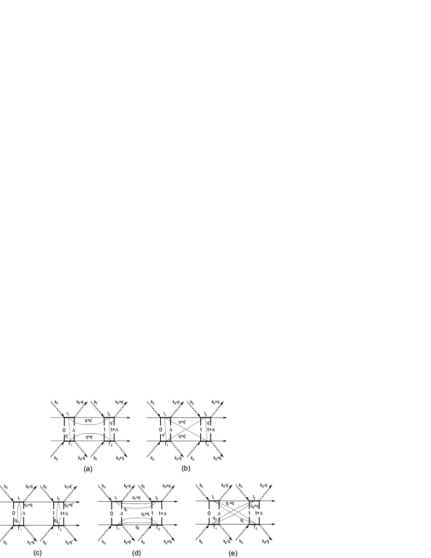
Figure 2: Double-sided Feynman diagrams for scattering process of photon with electric dipole moment (phonon). The photons and phonons are denoted by the wavy and dashed lines, respectively. In each diagram, the upper and lower horizontal time lines represent the bra and ket vectors, respectively.

II.3 Dynamics of crystal

A mathematically tractable approach to spectral function $A_{q}(\omega)$ is to introduce an imaginary time phonon Green’s function, for it can be evaluated more easily than its real time counterpart. In the real space, the imaginary time Green’s function is defined as,

$$G_{ll^{\prime\prime}}(\tau)\equiv-2\langle\langle T\hat{Q}_{l}(\tau)\hat{Q}_{l^{\prime\prime}}(0)\rangle\rangle,$$ (20)

where $\tau$ ($\equiv it$) is the argument for imaginary time (in this paper, we follow a convention of using Roman $t$ for real time and Greek $\tau$ for imaginary time). The imaginary time dependence of an operator in the interaction representation is given by

$$\hat{O}(\tau)=e^{\tau H_{0}}Oe^{-\tau H_{0}}.$$ (21)

Under the weak coupling approximation, and by using the Suzuki-Trotter identity, the Green’s function can be rewritten into a path integral form (here we assume $\tau$$>$0),ji04

$$G_{ll^{\prime\prime}}(\tau)=\int{\mathcal{D}}xe^{-\beta[\Phi_{f}(x)-\Phi_{f}]}[-2x_{l}(\tau)x_{l^{\prime\prime}}(0)],$$ (22)

where $x_{l}$ is the eigenvalue of $Q_{l}$,

$$Q_{l}|x_{l}\rangle=x_{l}|x_{l}\rangle,$$ (23)

$\Phi_{f}(x)$ is the path-dependent phonon free energy

$$e^{-\beta\Phi_{f}(x)}=e^{-\int_{0}^{\beta}d\tau\Omega_{f}[x(\tau)]},$$ (24)

with

$$\Omega_{f} = \sum_{l}\left[{1\over 2\omega_{0}}\left({\partial x_{l}\over\partial\tau}\right)^{2}+{1\over 2}\omega_{0}x_{l}^{2}-{1\over 2}\omega_{0}c_{4}x_{l}^{4}\right.$$ (25)

$$\left.+{1\over 6}\omega_{0}c_{6}x_{l}^{6}\right]-{1\over 2}\omega_{0}d_{2}\sum_{\langle l,l^{\prime}\rangle}x_{l}x_{l^{\prime}},$$

and $\Phi_{f}$ is the total phonon free energy,

$$e^{-\beta\Phi_{f}}=\int{\mathcal{D}}xe^{-\beta\Phi_{f}(x)}.$$ (26)

In the path integral notation, the internal energy of crystal $E_{f}$ ($\equiv\langle\langle H_{f}\rangle\rangle$) is represented as

$$E_{f} = \int{\mathcal{D}}xe^{-\beta[\Phi_{f}(x)-\Phi_{f}]}\left[\omega_{0}\sum_{l}\left(x_{l}^{2}-{3\over 2}c_{4}x_{l}^{4}\right.\right.$$ (27)

$$\left.\left.+{2\over 3}c_{6}x_{l}^{6}\right)-\omega_{0}d_{2}\sum_{\langle l,l^{\prime}\rangle}x_{l}x_{l^{\prime}}\right],$$

from which the heat capacity can be derived as

$$C_{f}^{V}=\left({\partial E_{f}\over\partial T}\right)_{V}.$$ (28)

The Green’s function of momentum space is given by,

$$G_{q}(\tau)={1\over N}\sum_{l,l^{\prime\prime}}e^{iq(l-l^{\prime\prime})}G_{ll^{\prime\prime}}(\tau),$$ (29)

which is connected with the phonon spectral function $A_{q}(\omega)$ throughbo96

$$G_{q}(\tau)=-\int_{0}^{\infty}{d\omega\over 2\pi}\frac{\cosh\left[\left({1\over 2}\beta-\tau\right)\omega\right]}{\sinh\left({1\over 2}\beta\omega\right)}A_{q}(\omega).$$ (30)

Solving this integral equation is a notoriously ill-posed numerical problem because of the highly singular nature of the kernel. In order to analytically continue the imaginary time data into real frequency information, specialized methods are developed, such as maximum entropy methodsk84 and least squares fitting method.ya03 In present work, we adopt the iterative fitting approach,ji04 for it can give a rapid and stable convergence of the spectrum without using any prior knowledge or artificial parameter. Since the phonon spectral function does not yield a specific sum rule like the case of electron, here we introduce an auxiliary spectral function $\tilde{A}_{q}(\omega)$ which is defined by

$$\tilde{A}_{q}(\omega)\equiv-\frac{\coth\left({1\over 2}\beta\omega\right)}{G_{q}(\beta)}A_{q}(\omega).$$ (31)

Substituting $\tilde{A}_{q}(\omega)$ into Eq. (30), we get

$$G_{q}(\tau)=\int_{0}^{\infty}{d\omega\over 2\pi}\frac{\cosh\left[\left({1\over 2}\beta-\tau\right)\omega\right]}{\cosh\left({1\over 2}\beta\omega\right)}G_{q}(\beta)\tilde{A}_{q}(\omega).$$ (32)

It can be easily shown that this auxiliary spectral function satisfies a sum rule,

$$\int_{0}^{\infty}{d\omega\over 2\pi}\tilde{A}_{q}(\omega)=1,$$ (33)

which allow us to solve the integral equation of Eq. (32) by the iterative fitting approach. Once $\tilde{A}_{q}(\omega)$ is reproduced, the phonon spectral function $A_{q}(\omega)$ can be obtained from Eq. (31).

III Numerical results and discussion

III.1 Optical responses

Based on the path integral formalisms, the imaginary time Green’s function can be readily calculated via a standard quantum Monte Carlo simulation.ji04 Our numerical calculation is performed on a 10$\times$10$\times$10 cubic lattice with a periodic boundary condition. The imaginary time is discretized into 10-20 infinitesimal slices. As already noticed for the analytic continuation,gu91 if the imaginary time Green’s function is noisy, the uncertainty involved in the inverse transform might be very large, and the spectral function cannot be determined uniquely. In order to obtain accurate data from quantum Monte Carlo simulation, a hybrid algorithmji04 has been implemented in our calculation. Besides, we pick out each Monte Carlo sample after 100-200 steps to reduce the correlation between adjacent configurations. The Monte Carlo data are divided into 5-10 sets, from which the 95% confidence interval is estimated through 10,000 resampled set averages by the percentile bootstrap method. We found that about 1,000,000 Monte Carlo configurations are sufficient to get well converged spectral functions and real time dynamic quantities.

Figure 3: On-site potential $U_{0}$ for the modified Krumhansl-Schrieffer model in the unit of $\omega_{0}$. The coordinates of potential extrema are denoted by $x_{a}$, $x_{b}$, and $x_{c}$. $\delta$ and $\xi$ are two parameters adopted to characterize this potential.

In the numerical calculation, the phonon frequency $\omega_{0}$ is assumed to be 20 meV,zh94 the inter-site coupling constant $d_{2}$ is fixed at a value of 0.032, whereas $c_{4}$ and $c_{6}$ are selected to make the on-site $U_{0}$ a symmetric triple-well potential. As shown in Fig. 3, this triple-well structure is featured by five potential extrema located at $x_{a}$, $\pm x_{b}$ and $\pm x_{c}$, where

$$x_{a} = 0,$$ (34)

$$x_{b} = \sqrt{\frac{c_{4}-\sqrt{c^{2}_{4}-c_{6}}}{c_{6}}},$$ (35)

$$x_{c} = \sqrt{\frac{c_{4}+\sqrt{c^{2}_{4}-c_{6}}}{c_{6}}}.$$ (36)

Figure 4: Phonon spectral function along the line $\Gamma$XMR of Brillouin zone in the paraelectric phase at various temperatures: (a) 1.001$T_{c}$, (b) 1.012$T_{c}$, (c) 1.059$T_{c}$, and (d) 1.176$T_{c}$, where $T_{c}$=386 K. The inset of panel (a) shows the Brillouin zone with high symmetry lines. The inset of panel (b) represents the spectrum at $\Gamma$ point when $T$=1.012$T_{c}$. Error bars mark the 95% confidence interval.

In Figs. 4 and 5, we show the optical responses of crystal, where $c_{4}$=2.0132$\times$10^-2 and $c_{6}$=3.2595$\times$10^-4 are used. Fig. 4 presents the phonon spectral functions in the paraelectric phase at different temperatures: (a) $T$=1.001$T_{c}$, (b) $T$=1.012$T_{c}$, (c) $T$=1.059$T_{c}$ and (d) $T$=1.176$T_{c}$, where $T_{c}$=386 K. In each panel, the spectra are arranged with wave vectors along the $\Gamma$XMR direction of Brillouin zone [see in the inset of panel (a)], and $\omega$ refers to energy. In the inset of panel (b), the spectrum at $\Gamma$ point for $T$=1.012$T_{c}$ is plotted with 95% confidence interval illustrated by the error bars. Since the spectra are symmetric with respect to the origin $\omega$=0, here we only show the positive part of them. In Fig. 4, when the temperature decreases towards $T_{c}$, as already well-known for the displacive type phase transition, the energy of phonon peak is gradually softened. In addition, a so-called central peak, corresponding to the low energy excitation of ferroelectric cluster, appears at the $\Gamma$ point. The collective excitation represented by this sharp resonant peak is nothing but the photo-created ferroelectric cluster. On decreasing temperature, spontaneous polarization is developed locally as a dipole fluctuation in the paraelectric phase. This fluctuation can stabilize the photo-created ferroelectric cluster, leading to a dramatically enhanced peak intensity near $T_{c}$.

The appearance of sharp peak at $\Gamma$ point nearby $T_{c}$ signifies a long life-time of the photo-created ferroelectric clusters after irradiation. Thus, near $T_{c}$, they are more likely to be probed by subsequent laser pulse, resulting in a high intensity of speckle pattern. Keeping this in mind, we move on to the results of scattering probability. In Fig. 5, we show the variation of normalized probability $P(t)/P(0)$ as a function of $t$ (time interval between the pump and probe photons). Temperatures for these curves correspond to those in the panels (a)-(d) of Fig. 4, respectively. In this figure, $P(t)/P(0)$ declines exponentially, showing that the speckle correlation decreases with $t$ increases as a result of the photorelaxation of ferroelectric cluster. When $t$ is long enough, the crystal returns to the equilibrium paraelectric state. In addition, as shown in the figure, the relaxation rate bears a temperature dependence. On approaching $T_{c}$, the duration for return is prolonged, indicative of a critical slowing down of the relaxation. This is because with the decrease of temperature, the fluctuation of local polarization is enhanced, and a long range correlation between dipole moments is to be established as well, making the relaxation of photo-created clusters slower and slower.

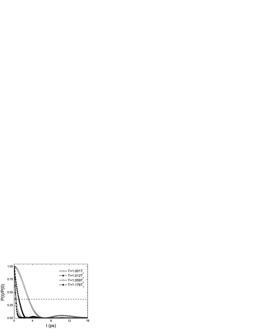
Figure 5: Normalized speckle scattering probability as a function of time for paraelectric BaTiO₃, at various temperatures. Horizontal dashed line denotes $P(t)=P(0)/e$.

III.2 Critical slowing down of photorelaxation

In order to quantitatively depict the critical slowing down, we introduce a relaxation time $t_{r}$ to estimate the time scale of relaxation, which is the time for $P(t)$ to be reduced by a factor of $e$ from $P(0)$. In Fig. 5, $P(t)$=$P(0)/e$ is plotted by a horizontal dashed line. Correspondingly, $t_{r}$ is the abscissa of the intersection point of relaxation curve and this dashed line. In Fig. 6, the relaxation time for various local potential $U_{0}$ is presented at $T>T_{c}$. Here we adopt two legible parameters, $\delta$ and $\xi$, to describe the potential wells and barriers for $U_{0}$ (see Fig. 3), which are defined by

$$\delta \equiv [U_{0}(x_{b})-U_{0}(x_{c})]/\omega_{0},$$ (37)

$$\xi \equiv U_{0}(x_{c})/\omega_{0}.$$ (38)

Provided $\delta$ and $\xi$, $c_{4}$ and $c_{6}$ can be derived in terms of Eqs. (35)-(38). The values of $c_{4}$ and $c_{6}$ for the calculation of Fig. 6 are listed in Table I, where we set $\xi$=3.061 and change $\delta$ from 4.239 to 4.639. The leftmost point on each curve denotes the $t_{r}$ at just above $T_{c}$, which is a temperature determined from the singular point of $C_{f}^{V}$ according to Eq. (28).

Figure 6: Temperature dependence of relaxation time $t_{r}$ for various $\delta$ when $T>T_{c}$, where $\xi$ is fixed at 4.439. Error bars show the 95% confidence interval.

As revealed by the NMR experiment,za03 the paraelectric-ferroelectric phase transition of BaTiO₃ has both displacive and order-disorder components in its mechanism. Short range dipole fluctuation arises in the paraelectric phase near $T_{c}$ as a precursor of the order-disorder transition, and condenses into long range ferroelectric ordering below $T_{c}$. Thus, in the present study, the relaxation of photo-created cluster is also subject to the dynamics of this dipole fluctuation and yields a temperature dependence. As illustrated by the three curves in Fig. 6, if a ferroelectric cluster is created at a temperature close to $T_{c}$, relaxation of this cluster is slow because of a rather strong dipole fluctuation, which holds the cluster in the metastable ferroelectric state from going back to the paraelectric one. Away from $T_{c}$, $t_{r}$ decreases considerably for the dipole fluctuation is highly suppressed. This behavior is nothing but the critical slowing down of photorelaxation.

Table 1: Parameters adopted for calculation of Fig. 6.

$c_{4}$	$c_{6}$	$\delta$	$\xi$	$T_{c}$ (K)
2.0696$\times$10-2	3.4521$\times$10-4	4.239	3.061	340
2.0132$\times$10-2	3.2593$\times$10-4	4.439	3.061	386
1.9596$\times$10-2	3.0814$\times$10-4	4.639	3.061	422

In Fig. 6, it can also be seen that with the increase of $\delta$, $T_{c}$ moves to the high temperature side so as to overcome a higher potential barrier between the ferroelectric and paraelectric phases. Furthermore, the evolution of $t_{r}$ becomes gentle as well, implying a gradual weakening of dipole fluctuation at high temperature region.

Figure 7: Temperature dependence of relaxation time $t_{r}$ for various $\xi$ when $T>T_{c}$, where $\delta$ is fixed at 3.061. Error bars show the 95% confidence interval.

Table 2: Parameters adopted for calculation of Fig. 7.

$c_{4}$	$c_{6}$	$\delta$	$\xi$	$T_{c}$ (K)
1.9626$\times$10-2	3.1070$\times$10-4	4.439	3.261	354
2.0132$\times$10-2	3.2593$\times$10-4	4.439	3.061	386
2.0663$\times$10-2	3.4223$\times$10-4	4.439	2.861	404

In Fig. 7, we show the temperature dependence of $t_{r}$ for different $\xi$ when $T>T_{c}$, where $\delta$ is fixed at 4.439. The values of parameters for this calculation are given in Table II. When $\xi$ changes from 3.261 to 2.861, as shown in Fig. 7, $T_{c}$ gradually increases. This is because with the decrease of $\xi$, the ferroelectric state at $x_{c}$ (refer to Fig. 3) becomes more stable and can survive even larger thermal fluctuation. In a manner analogous to Fig. 6, the evolution of $t_{r}$ also displays a sharp decline at low temperature, and becomes more and more smooth as temperature increases.

Figure 8: Temperature dependence of relaxation time $t_{r}$ for various barrier height $\delta+\xi$ when $T>T_{c}$, where $\delta/\xi$=1.5 is assumed. Error bars show the 95% confidence interval.

In Fig. 8, we plot the temperature dependence of $t_{r}$ for different barrier heights, i.e., $\delta+\xi$ varies from 7.0 to 8.0, while the ratio $\delta/\xi$ is fixed at 1.5. Parameters for this calculation are provided in Table III. As already discussed with Figs. 6 and 7, larger $\delta$ tends to increases $T_{c}$, but higher $\xi$ applies an opposite effect on $T_{c}$. Combining these two effects, in Fig. 8, one finds that $T_{c}$ increases if both $\delta$ and $\xi$ are enhanced, indicating that in this case, the change of $\delta$ plays a more significant role. Meanwhile, in contrast to Figs. 6 and 7, all the three curves in Fig. 8 present smooth crossovers on decreasing temperature towards $T_{c}$, signifying that dipole fluctuation can be promoted by lowering $\xi$ even the temperature is decreased.

Table 3: Parameters adopted for calculation of Fig. 8.

$c_{4}$	$c_{6}$	$\delta$	$\xi$	$\delta+\xi$	$T_{c}$ (K)
2.1557$\times$10-2	3.7309$\times$10-4	4.200	2.800	7.000	372
2.0122$\times$10-2	3.2505$\times$10-4	4.500	3.000	7.500	400
1.8860$\times$10-2	2.8557$\times$10-4	4.800	3.200	8.000	436

In Namikawa’s experiment, the wavelength of soft x-ray laser is 160 Å, hence the photo-created cluster is of nano scale. However, it should be noted that relaxation of nano-sized cluster is beyond our present quantum Monte Carlo simulation because of the size limitation of our model. This is the primary reason why the experimentally measured relaxation time can reach about 30 picoseconds, being several times longer than our calculated results. In spite of the difference, our calculation has well clarified the critical dynamics of BaTiO₃ and the origin of speckle variation.

IV Summary

We carry out a theoretical investigation to clarify the dynamic property of photo-created ferroelectric cluster observed in the paraelectric BaTiO₃ as a real time correlation of speckle pattern between two soft x-ray laser pulses. The density matrix is calculated by a perturbative expansion up to the fourth order terms, so as to characterize the time dependence of scattering probability. The cluster-associated phonon softening as well as central peak effects are well reproduced in the phonon spectral function via a quantum Monte Carlo simulation. We show that the time dependence of speckle pattern is determined by the relaxation dynamics of photo-created ferroelectric cluster, which is manifested as a central peak in the phonon spectral function. The photorelaxation of ferroelectric cluster is featured by a critical slowing down on decreasing the temperature. Near the $T_{c}$, cluster excitation is stablized by the strong dipole fluctuation, correspondingly the relaxation becomes slow. While, at higher temperature, dipole fluctuation is suppressed, ending up with a quicker relaxation of cluster. Our simulation also illustrates that the critical slowing down and dipole fluctuation are subject to the chemical environment of crystal.

V Acknowledgments

This work is supported by the Next Generation Supercomputer Project, Nanoscience Program, MEXT, Japan.

References

- (1) M. May, J. Phys. E 10 849 (1977).
- (2) J. W. Goodman, Speckle Phenomena in Optics: Theory and Applications (Roberts and Company, Greenwood Village, 2007).
- (3) R. Z. Tai, K. Namikawa, M. Kishimoto, M. Tanaka, K. Sukegawa, N. Hasegawa, T. Kawachi, M. Kado, P. Lu, K. Nagashima, H. Daido, H. Maruyama, A. Sawada, M. Ando, and Y. Kato, Phys. Rev. Lett. 89, 257602 (2002).
- (4) R. Z. Tai, K. Namikawa, A. Sawada, M. Kishimoto, M. Tanaka, P. Lu, K. Nagashima, H. Maruyama, and M. Ando, Phys. Rev. Lett. 93, 087601 (2004).
- (5) S.-I. Hamazaki, F. Shimizu, S. Kojima, and M. Takashige, J. Phys. Soc. Jpn. 64 3660 (1995).
- (6) G. K. H. Pang and K. Z. Baba-Kishi, J. Phys. D 31 2846 (1998).
- (7) Y. Yamada, G. Shirane, and A. Linz, Phys. Rev. 177 848 (1969).
- (8) W. L. Mulvihill, K. Uchino, Z. Li and W. Cao, Phil. Mag. B 74 25 (1996).
- (9) D. L. Polla and L. F. Francis, Annu. Rev. Mater. Sci. 28 563 (1998).
- (10) J. Harada, J. D. Axe, and G. Shirane, Phys. Rev. B 4 155 (1971).
- (11) R. Migoni, D. Bauer, and H. Bilz, Phys. Rev. Lett. 37 1155 (1976).
- (12) B. Zalar, V. V. Laguta, and R. Blinc Phys. Rev. Lett. 90 037601 (2003).
- (13) G. Völkel and K. A. Müller, Phys. Rev. B 76 094105 (2007).
- (14) K. Namikawa, unpublished.
- (15) R. Yan, Z. Guo, R. Tai, H. Xu, X. Zhao, D. Lin, X. Li, and H. Luo, Appl. Phys. Lett. 93, 192908 (2008).
- (16) J. A. Krumhansl and J. R. Schrieffer, Phys. Rev. B 11, 3535 (1975).
- (17) S. Aubry, J. Chem. Phys. 62 3217 (1975).
- (18) T. Schneider and E. Stoll, Phys. Rev. B 17, 1302 (1978).
- (19) V. V. Savkin, A. N. Rubtsov, and T. Janssen, Phys. Rev. B 65 214103 (2002).
- (20) J. R. Morris and R. J. Gooding, Phys. Rev. Lett. 65, 1769 (1990).
- (21) A. Khare, A. Saxena, J. Math. Phys. 49, 063301 (2008).
- (22) K. Nasu, J. Phys. Soc. Jpn. 63, 2416 (1994).
- (23) S. Doniach and E. H. Sondheimer, Green’s Function for Solid State Physicists, (Benjamin, London, 1974), Appendix 2.
- (24) K. Ji, H. Zheng, and K. Nasu, Phys. Rev. B 70, 085110 (2004).
- (25) J. Bonča and J. E. Gubernatis, Phys. Rev. B 53, 6504 (1996).
- (26) Skilling and R. K. Bryan, Mon. Not. R. Astron. Soc. 211, 111 (1984).
- (27) M. Yamazaki, N. Tomita, and K. Nasu, J. Phys. Soc. Jpn. 72, 611 (2003).
- (28) J. E. Gubernatis, M. Jarrell, R. N. Silver, and D. S. Sivia Phys. Rev. B 44, 6011 (1991).
- (29) W. Zhong, R. D. King-Smith, and D. Vanderbilt, Phys. Rev. Lett. 72, 3618 (1994).