Soft disks in a narrow channel

Abstract

The pressure components of ”soft” disks in a two dimensional narrow channel are analyzed in the dilute gas regime using the Mayer cluster expansion and molecular dynamics. Channels with either periodic or reflecting boundaries are considered. It is found that when the two-body potential, $u(r)$, is singular at some distance $r_{0}$, the dependence of the pressure components on the channel width exhibits a singularity at one or more channel widths which are simply related to $r_{0}$. In channels with periodic boundary conditions and for potentials which are discontinuous at $r_{0}$, the transverse and longitudinal pressure components exhibit a $1/2$ and $3/2$ singularity, respectively. Continuous potentials with a power law singularity result in weaker singularities of the pressure components. In channels with reflecting boundary conditions the singularities are found to be weaker than those corresponding to periodic boundaries.

I Introduction

The thermodynamic and dynamical properties of particles in restricted geometries are of great interest. They have been extensively studied in the context of porous media Given ; Konig ; Evans ; Smit , transport through narrow channels such as carbon nanotubes Hummer ; Allen and pores in biological membranes Hille as well as in numerous other systems Gelb . Perhaps the simplest and most convenient theoretical approach for studying fluids in cavities models the fluid by hard spheres. This approach has been applied in a large number of studies (see for example, Kamenetskiy ; Kim ; Mon2000 ; Kofke ; Klafter ). Recent studies of a dilute gas of hard disks in a narrow two dimensional channel have shown that the system exhibits a singularity in the pressure at a channel width equal to twice the diameter of the disks FMP04 ; Bowles . This is a consequence of the fact that the volume of the phase space available to the disks exhibits a singularity at this width. In particular, it has been found that for a channel with periodic boundary condition, the transverse component of the pressure exhibits a $3/2$ singularity, while the longitudinal component exhibits a $5/2$ singularity FMP04 . In the case of a channel with reflecting boundaries, weaker singularities for both pressure components were found Bowles .

In this paper we extend these studies to consider a gas of ”soft” disks in a narrow channel at low density. We consider several classes of two body potentials, with both periodic and reflecting channel boundaries. Our analysis shows that the pressure components are singular at some channel widths whenever the interaction potential between two disks, $u(r)$, is singular at some distance $r_{0}$. In particular, in the case of periodic boundary conditions and for potentials which are discontinuous at some $r_{0}$, the dependence of the transverse component of the pressure on the channel width exhibits a $1/2$ singularity, while the longitudinal component exhibits a $3/2$ singularity at some channel widths, which are simply related to $r_{0}$. The nature of these singularities becomes weaker for interaction potentials which are continuous, but they still display a power law singularity at $r_{0}$. The singularities of the case of reflecting boundary conditions are found to be weaker than those corresponding to periodic boundaries. Although we have not analyzed narrow channels in three dimensions, we expect similar phenomena to take place there as well. The nature of the singularities in the pressure in three dimensions is expected to be different from that of the two dimensional case.

In the following sections we study several classes of two body potentials $u(r)$ for both periodic and reflecting boundary conditions. In Section II we present the general formulation of the tools used in this study, the Mayer cluster expansion for gases at low densities, and molecular dynamics. In Section III we analyze the case of a channel with periodic boundary conditions, for one-step and two-steps potentials. We also study a smooth potential which vanishes with a power law at a critical distance. In Section IV we study a channel with reflecting boundaries for the cases of soft disks and soft disks with a hard core. Finally, a brief summary is given in Section V.

II General Formulation

We consider $N$ disks of diameter $d$ and mass $m$, interacting via a two body potential $u(r)$ at temperature $T$. The disks are restricted to move in a channel of length $L_{x}$ and width $L_{y}$ with $L_{y}\ll L_{x}$. In this study we analyze the pressure components of this gas using virial expansion to second order in the density. We also carry out molecular dynamics simulations of this system. In the present study the channel width, $L_{y}$, is taken to be finite throughout the calculation. Therefore the free energy is not extensive in $L_{y}$ and, thus, Euler’s relation does not hold, namely, $-PV\neq E-TS-\mu N$. Thus, the pressure has to be calculated by taking the appropriate derivative of the free energy.

In the grand canonical ensemble the free energy of a system of $N$ disks is given by

$$F(T,V,N) = -kT\ln{{\mathcal{L}}(T,V,z)}+kTN\ln{z}\;,$$

$$N = z{\frac{\partial}{\partial z}}\ln{{\mathcal{L}}(T,V,z)}\;.$$ (1)

Here ${\mathcal{L}}$ is the grand partition sum, $z$ is the fugacity, $k$ is the Boltzmann constant and $V=L_{x}L_{y}$. The pressure components are evaluated by taking the appropriate derivatives of the free energy

$$P_{xx}V = -L_{x}{\frac{\partial F}{\partial L_{x}}}$$

$$P_{yy}V = -L_{y}{\frac{\partial F}{\partial L_{y}}}$$

$$P = {\frac{1}{2}}(P_{xx}+P_{yy})\;.$$ (2)

To second order in the fugacity $z$, the Mayer expansion yields

$$\ln{\mathcal{L}} = {\frac{V}{\lambda^{2}}}(b_{1}z+b_{2}z^{2})$$

$${\frac{1}{v}}\equiv{\frac{N}{V}} = {\frac{1}{\lambda^{2}}}(b_{1}z+2b_{2}z^{2})\;,$$ (3)

where $\lambda=h/\sqrt{2\pi mkT}$ is the average thermal wavelength and $h$ is Planck’s constant. The coefficients of the expansion satisfy

$$b_{1} = 1$$

$$b_{2} = {\frac{1}{2\lambda^{2}}}q(L_{y})\;,$$ (4)

with

$$q(L_{y})=\int f_{12}d^{2}{r_{12}}~{}.$$ (5)

Here, $f_{12}=e^{-\beta u(r_{12})}-1$ is the Mayer function, and $\beta=1/kT$. Using Eqs. (1,3) we find that to order $1/v$ the free energy is given by

$$\frac{F}{kTN}=-1-{\frac{q(L_{y})}{2v}}-\ln{v}+2\ln{\lambda}\quad,$$ (6)

from which the components of the pressure tensor are obtained:

$$\frac{P_{xx}v}{kT} = 1-\frac{q{(L_{y})}}{2v}\,,$$ (7)

$$\frac{P_{yy}v}{kT} = 1-\frac{q{(L_{y})}}{2v}+\frac{L_{y}}{2v}\frac{dq(L_{y})}{dL_{y}}\;.$$ (8)

All theoretical considerations are augmented by computer simulations. For our two-dimensional systems, the temperature $T$ is computed from

$$\langle K\rangle=\left(N-\frac{g}{2}\right)kT,$$ (9)

where $K$ is the kinetic energy and the bracket denotes a time average. Here, $g$ is the number of macroscopic conservation laws, which differs for the periodic boundaries of Section III, $(g=3$; the total momentum is constant and is taken to vanish), and for the reflecting boundaries used in Section IV $(g=1)$. The diagonal elements of the pressure tensor, $P_{\alpha\alpha}$ for $\alpha\in\{x,y\}$, are evaluated from the virial theorem,

$$P_{\alpha\alpha}V=\langle K\rangle+W_{\alpha\alpha}.$$ (10)

For impulsive interactions Rapaport , the potential contribution, $W_{\alpha\alpha}$, is given by

$$W_{\alpha\alpha}=\frac{1}{\tau}\sum_{c}r_{\alpha,ij}^{(c)}\Delta v_{\alpha,i}^{(c)}\;,$$ (11)

Here, the sum is over all collisional events $c$, which instantaneously change the potential energy during the averaging time $\tau$, $r_{\alpha,ij}^{(c)}\equiv r_{\alpha,i}^{(c)}-r_{\alpha,j}^{(c)}$ is the $\alpha$-component of the separation vector of the two particles involved in the event, and $\Delta v_{\alpha,i}^{(c)}$ denotes the velocity change for particle $i$ parallel to $\alpha$ due to that event (the velocity change for particle $j$ being just the opposite). For the continuous potentials of Section III.3, the potential contribution becomes

$$W_{\alpha\alpha}=\frac{1}{\tau}\int_{0}^{\tau}dt\sum_{i}\sum_{j>i}r_{\alpha,ij}f_{\alpha,ij}\;,$$ (12)

where $f_{\alpha,ij}$ is the $\alpha$-component of the force exerted on $i$ by particle $j$. In all figures comparing experimental with theoretical pressures, the experimental dots represent $W_{\alpha\alpha}/\langle K\rangle$. The theoretical smooth curves represent $(P_{\alpha\alpha}v/kT)-1$, where the temperature required for this computation is taken from Eq. (9). As usual, temperature units are used, for which Boltzmann’s constant $k$ is unity. Because of the equivalence of the canonical and microcanonical ensembles, the experimental and theoretical pressures should agree up to a term of order O$(1/N)$. To make this correction insignificant, at least 60 particles, or even 120 in many cases, were used for the simulations.

An event-driven algorithm is used Rapaport ; AT for the discontinuous potentials with periodic (Sec. III) or reflecting (Sec. IV) boundary conditions, for which instantaneous potential energy changes and boundary crossings of a particle are considered as events. For the continuous power-law potentials of Sec. III.3 a hybrid code is used, which will be described there in more detail.

III Narrow channels with periodic boundary conditions

III.1 Positive step potential

We proceed by considering the pressure in the case of a two-body step potential

$$u(r)=\left\{\begin{array}[]{ll}u&\qquad r\leq d\\ 0&\qquad r>d\,,\end{array}\right.$$ (13)

where $u>0$ is a constant (in our previous paper FMP04 we considered the hard-disk case $u=\infty$). The case $u<0$ is pathological, since the particles may collapse to form a cluster, as long as there is no repulsive interaction at short distances. The case of a two step potential with repulsion at short distances and attraction at larger distances will be considered in the following sub-section. Here we limit ourselves to the repulsive potential case $u>0$. To evaluate the pressure we associate with each particle an interaction disk of radius $d$ centered at its position. Two particles $i$ and $j$ interact with each other, if the center of $j$ is within the interaction disk of $i$, and vice versa. In the case $L_{y}>2d$ the cross sections of a particle (a disk of radius d) and that of its image resulting from the periodic boundary conditions in the $y$ direction do not overlap. Hence the integral (5) simply yields

$$q(L_{y})=\pi d^{2}(e^{-\beta u}-1)\qquad\mbox{for}\qquad L_{y}>2d\,.$$ (14)

For $L_{y}<2d$ we note that the area of overlap between the interaction disk of a particle and that of its image translated in the $y$ direction is given by

$$S(\vartheta)=d^{2}(\pi-2\vartheta-\sin{2\vartheta})\>,$$ (15)

where $\vartheta$ satisfies (see Fig. (1))

$$L_{y}=2d\sin\vartheta\,.$$ (16)

In this case the integral (5) yields

$$q(L_{y})=(\pi d^{2}-2S(e^{-\beta u}-1)+S(e^{-2\beta u}-1)\;.$$ (17)

Figure 1: The interaction disks arrangement for $L_{y}<2d$ with periodic boundary conditions. The overlap area of the two disks is $S$.

Using this result for $q(L_{y})$, and noting that

$$\frac{dS}{dL_{y}}=-\sqrt{4d^{2}-L_{y}^{2}}~{}\quad,$$ (18)

it is straightforward to derive the expressions for the pressure. We find that to order $1/v$ and for $L_{y}>2d$ one has $P_{xx}=P_{yy}=P$ with

$$\frac{Pv}{kT}=1-\frac{q}{2v}\,,$$ (19)

where $q$ is independent of $L_{y}$ and is given by (14). On the other hand, for $L_{y}<2d$ one finds

$$\frac{P_{xx}v}{kT} = 1-\frac{q{(L_{y})}}{2v}\,,$$ (20)

$$\frac{P_{yy}v}{kT} = 1-\frac{q{(L_{y})}}{2v}-\frac{L_{y}}{2v}\sqrt{4d^{2}-L_{y}^{2}}\left(1-e^{-\beta u}\right)^{2}\;,$$ (21)

$$\frac{Pv}{kT} = 1-\frac{q{(L_{y})}}{2v}-\frac{L_{y}}{4v}\sqrt{4d^{2}-L_{y}^{2}}\left(1-e^{-\beta u}\right)^{2}\>,\$$ (22)

where $q(L_{y})$ is given by (17). It is evident that $P_{yy}$ exhibits a square-root singularity at $L_{y}=2d$ as in the case of hard disks FMP04 . This singularity originates from the term $dq(L_{y})/dL_{y}$ in (8). On the other hand, $P_{xx}$ exhibits a weaker singularity with a singular term which vanishes as $(2d-L_{y})^{3/2}$. The reason is that unlike the $P_{yy}$ component, here the singularity originates from $q(L_{y})$ and not from its derivative. Clearly, the pressure $P$, which is the average of the two components, exhibits a square-root singularity as the more singular $P_{yy}$ component.

Figure 2: Comparison of the channel-width dependence of the theoretical pressures (lines) with numerical simulations (points) for a system of 60 disks interacting with the step potential of Eq. (13). The density is kept constant, $N/V=0.01$. The potential varies from $u=0.5$ (top) to $u=2$ (bottom). The singularities appear at $L_{y}=2$ and $L_{y}=1$ as explained in the main text. Reduced units are used, for which $d$ and the total energy per particle, $E/N$, are unity.

In Fig. 2 the theoretical expressions for the singularity at $L_{y}=2d=2$ are compared to computer simulation results for various potential step sizes $u$ as indicated by the labels. Reduced units are used for which the particle diameter $d$ and the total energy per particle, $E/N$, are unity. The energy $E/N$ is almost exclusively kinetic in nature with a time-averaged kinetic temperature $T=0.986$ for $u=0.5$ (top), $T=0.994$ for $u=1.0$ (middle), and $T=0.996$ for $u=2$ (bottom figure). These temperatures vary slightly, but insignificantly, with the channel width $L_{y}$. The density is kept constant, $N/V=0.01$. As for the case of hard spheres ($u=\infty$) treated already in Ref. FMP04 , the agreement between theory and simulation results is very satisfactory.

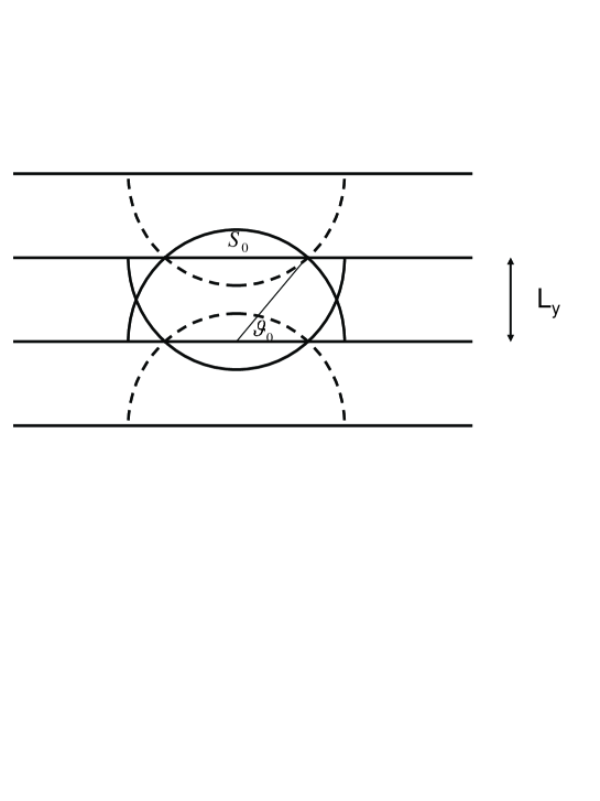
Figure 3: The interaction disks arrangement for $L_{y}<d$ with periodic boundary conditions. The overlap area of the disk and its next nearest neighbor in the $y$ direction is $S_{0}$.

As the width of the channel further decreases we expect to have more singularities to take place at $L_{y}=d,~{}2d/3,~{}d/2,\dots$, which result from the overlap of an interaction disk with those of further neighboring disks in the $y$ direction. Let us analyze, for example, the second singularity in the pressure curve, which takes place at $L_{y}=d$. For $d/2<L_{y}<d$ the disk of a particle has some overlap with its nearest and next nearest neighbors images which result from the periodic boundary conditions in the $y$ direction. In order to evaluate the overlap integral (5) we note that (see Fig. 3)

$$L_{y}=d\sin\vartheta_{0}\,.$$ (23)

The overlap area between an interaction disk of a particle and that of its next nearest neighbor in the $y$ direction, $S_{0}$, is given by

$$S_{0}=d^{2}(\pi-2\vartheta_{0}-\sin{2\vartheta_{0}})\,.$$ (24)

The overlap integral is thus expressed as

$$q(L_{y})=(\pi d^{2}-2S+S_{0})(e^{-\beta u}-1)+(S-2S_{0})(e^{-2\beta u}-1)+S_{0}(e^{-3\beta u}-1)\;.$$ (25)

Using this expression for the overlap integral, the pressure components can readily be calculated to yield

$$\frac{P_{xx}v}{kT} = 1-\frac{q{(L_{y})}}{2v}\;$$ (26)

$$\frac{P_{yy}v}{kT} = 1-\frac{q{(L_{y})}}{2v}-\frac{L_{y}}{2v}\sqrt{4d^{2}-L_{y}^{2}}\;(1-e^{-\beta u})^{2}-\frac{2L_{y}}{v}\sqrt{d^{2}-L_{y}^{2}}\;e^{-\beta u}(1-e^{-\beta u})^{2}\;$$ (27)

$$P = \frac{1}{2}(P_{xx}+P_{yy})\;.$$ (28)

As is also shown in Figure 2, these expressions for the singularity at $L_{y}=d=1$ compare very well with simulation results. As before, reduced units are used for which $d$ and $E/N$ are unity. Note that as long as $u>0$ the coefficient of the singular term $\sqrt{d^{2}-L_{y}^{2}}~{}$ is positive, resulting in a positive compressibility just below $L_{y}=d$.

III.2 Two-step potential

In order to analyze the case of disks with an attractive potential, one has to add a repulsive interaction at short distances to prevent the collapse of the system into a macroscopic cluster. We thus consider in this section a two-step potential

$$u(r)=\left\{\begin{array}[]{ll}u_{1}&\qquad r\leq d\;,\\ u_{2}&\qquad d\leq r<D\;,\\ 0&\qquad r\geq D\;.\end{array}\right.$$ (29)

where $u_{1}>0$ represents a repulsive interaction, $u_{2}$ could be either positive or negative, and $D>d$ is the outer radius of $u_{2}$. To evaluate the pressure we associate with each particle two concentric interaction disks, one with radius $d$ and the other with radius $D$. Two particles only interact with each other, if the center of the second particle lies within the interaction disks of the first. It is easy to see that the degree of overlap of the disks of a particle and those of its nearest neighbor image resulting from the periodic boundary condition in the y direction are singular at $L_{y}=2D,\;d+D$, and $2d$. Thus, the pressure curve is expected to be singular at these three values of the channel’s width.

We now analyze the pressure curve in more detail and consider first the upper singularity at $L_{y}=2D$. For $L_{y}>2D$ the disks of a particle and those of its image do not overlap. Thus the integral (5) yields

$$q(L_{y})=\pi(D^{2}-d^{2})(e^{-\beta u_{2}}-1)+\pi d^{2}(e^{-\beta u_{1}}-1)\qquad\mbox{for}\qquad L_{y}>2D\,,$$ (30)

and $q$ is independent of $L_{y}$. As in the case of a single step potential, one finds that to leading order in $1/v$ the pressure tensor is isotropic, $P_{xx}=P_{yy}=P$, with

$$\frac{Pv}{kT}=1-\frac{q}{2v}\;.$$ (31)

For $d+D\leq L_{y}\leq 2D$, however, the outer disks of a particle and its periodic image overlap. As in the case of the single step potential, the overlap area $S$ is given by

$$S=D^{2}(\pi-2\vartheta-\sin{2\vartheta})\,,$$ (32)

where $\vartheta$ satisfies (see Fig. (1))

$$L_{y}=2D\sin\vartheta\,.$$ (33)

The resulting overlap integral (5)  for $d+D<L_{y}<2D$ is given by

$$q(L_{y})=(\pi D^{2}-\pi d^{2}-2S)(e^{-\beta u_{2}}-1)+\pi d^{2}(e^{-\beta u_{1}}-1)+S(e^{-2\beta u_{2}}-1)\,.$$ (34)

The pressure tensor in this regime is thus found to be

$$\frac{P_{xx}v}{kT} = 1-\frac{q{(L_{y})}}{2v}\,,$$ (35)

$$\frac{P_{yy}v}{kT} = 1-\frac{q{(L_{y})}}{2v}-\frac{L_{y}}{2v}\sqrt{4D^{2}-L_{y}^{2}}(1-e^{-\beta u_{2}})^{2}\,,$$ (36)

$$\frac{Pv}{kT} = 1-\frac{q{(L_{y})}}{2v}-\frac{L_{y}}{4v}\sqrt{4D^{2}-L_{y}^{2}}(1-e^{-\beta u_{2}})^{2}\,,$$ (37)

where $q(L_{y})$ is given by (34). As in the case of a single step potential, $P_{yy}$ exhibits a square root singularity, while $P_{xx}$ behaves more smoothly, with a weaker 3/2 power behavior at the transition. The compressibility below the transition is negative.

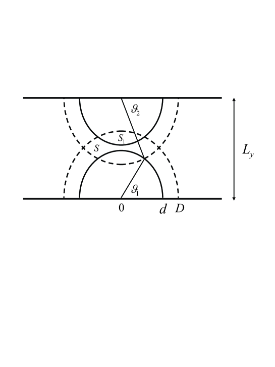
Figure 4: The interaction disks arrangement for the case of a two-step potential and for $2d\leq L_{y}\leq d+D$ with periodic boundary conditions. The overlap area of the outer disks of two nearest neighbors in the $y$ direction is $S_{1}$, while the overlap area of the outer disk with the inner one of its nearest neighbor in the $L_{y}$ direction is $S_{1}$. The angles $\vartheta_{1}$ and $\vartheta_{2}$ are indicated .

Finally, we consider the regime $2d\leq L_{y}\leq d+D$. In this case the outer disk of a particle partially overlaps not only with the outer disk of its periodic image but also with the inner one (see Fig. (4)). The overlap area $S_{1}$ between the outer and the inner disks is given by

$$S_{1}=\frac{1}{2}d^{2}(\pi-2\vartheta_{1})-d^{2}\sin\vartheta_{1}\cos\vartheta_{1}+\frac{1}{2}D^{2}(\pi-2\vartheta_{2})-D^{2}\sin\vartheta_{2}\cos\vartheta_{2}$$ (38)

where $\vartheta_{1}$ and $\vartheta_{2}$ satisfy (see Fig. (4))

$$L_{y}=d\sin\vartheta_{1}+D\sin\vartheta_{2}\,,\qquad\mbox{and}\qquad d\cos\vartheta_{1}=D\cos\vartheta_{2}\,,$$ (39)

and, hence,

$$\sin\vartheta_{1}=\frac{1}{2dL_{y}}(L_{y}^{2}-D^{2}+d^{2}),\qquad\sin\vartheta_{2}=\frac{1}{2DL_{y}}(L_{y}^{2}+D^{2}-d^{2})\,.$$ (40)

It is straightforward to express the overlap integral (5) in terms of the overlap areas $S$ and $S_{1}$ as

$$q(L_{y}) = (\pi D^{2}-\pi d^{2}-2S+2S_{1})(e^{-\beta u_{2}}-1)+(\pi d^{2}-2S_{1})(e^{-\beta u_{1}}-1)$$ (41)

$$+ (S-2S_{1})(e^{-2\beta u_{2}}-1)+2S_{1}(e^{-\beta(u_{1}+u_{2})}-1)\qquad\mbox{for}\qquad 2d\leq L_{y}\leq d+D\,.\,$$

According to Eqs. (7) and (8), the pressure components may be expressed as

$$\frac{P_{xx}v}{kT} = 1-\frac{q{(L_{y})}}{2v}\,,$$ (42)

$$\frac{P_{yy}v}{kT} = 1-\frac{q(L_{y})}{2v}+\frac{L_{y}}{2v}(1-e^{-\beta u_{2}})^{2}\frac{dS}{dL_{y}}+\frac{L_{y}}{v}(e^{-\beta u_{2}}-e^{-\beta u_{1}})(1-e^{-\beta u_{2}})\frac{dS_{1}}{dL_{y}}\,,$$ (43)

where

$$\frac{dS_{1}}{dL_{y}}=-2d\cos(\vartheta_{1})=-2D\cos(\vartheta_{2})\,.$$ (44)

Using Eq. (39) and (40), the channel-width dependence of the pressure tensor components for $2d<L_{y}<d+D$ is finally obtained,

$$\frac{P_{xx}v}{kT} = 1-\frac{q{(L_{y})}}{2v}\,,$$ (45)

$$\frac{P_{yy}v}{kT} = 1-\frac{q(L_{y})}{2v}-\frac{L_{y}}{2v}\sqrt{4D^{2}-L_{y}^{2}}(1-e^{-\beta u_{2}})^{2}-\frac{1}{v}(e^{-\beta u_{2}}-e^{-\beta u_{1}})(1-e^{-\beta u_{2}})$$ (46)

$$\times(4L_{y}^{2}D^{2}+4L_{y}^{2}d^{2}+4D^{2}d^{2}-L_{y}^{4}-D^{4}-d^{4})^{1/2}\,,$$

where $q(L_{y})$ is given by (41).

In order to establish the nature of the singularity at the transition point $d+D$, we expand $dS_{1}/dL_{y}$ in Eq. (44) in terms of the small dimensionless offset $\epsilon=(d+D-L_{y})/d$. Introducing the small angles

$$\vartheta_{1}=\frac{\pi}{2}-\delta\vartheta_{1}\,,\qquad\vartheta_{2}=\frac{\pi}{2}-\delta\vartheta_{2}\,,$$ (47)

which, according to Eq. (39), are related to $\epsilon$ by

$$(\delta\vartheta_{1})^{2}=\frac{2D}{(d+D)}\epsilon\,,\qquad(\delta\vartheta_{2})^{2}=\frac{2d^{2}}{D(d+D)}\epsilon\,,$$ (48)

we finally obtain

$$\frac{dS_{1}}{dL_{y}}=-d\sqrt{\frac{8D}{d+D}}\sqrt{\epsilon}$$ (49)

It is readily seen that $dS_{1}/dL_{y}$ and, hence, $P_{yy}$, exhibit a square root singularity. As in the case of a single step potential, the singularity in $P_{xx}$ originates from $S_{1}$ rather than from its derivative. Hence $P_{xx}$ exhibits a weaker $3/2$ singularity at $L_{y}=D+d$. It is interesting to note that, depending on the values of the interaction parameters $u_{1}$ and $u_{2}$, the compressibility just below the transition could be either positive or negative.

Figure 5: Channel-width dependence of the pressures for the two-step potential case with the following set of parameters: $d=1$, $D=1.5$, $N=60$, $N/V=0.01$ and $E/N=1$. The top panel corresponds to a potential with two positive steps, $u_{1}=2$ and $u_{2}=1$, whereas the lower panel is for an attractive outer shell with $u_{1}=2$ and $u_{2}=-1$.

In Fig. 5 we compare the respective theoretical expressions – Eq. (31) for $L_{y}>2D$, Eqs. (35 - 37) for $d+D<L_{y}<2D$, and Eqs. (45, 46) for $2d<L_{y}<d+D$ – to computer simulation results (dots) for $N=60$ particles in a narrow channel of width $L_{y}$ with periodic boundaries both in $x$ and $y$ directions. We use reduced units for which $E/N$ and $d$ are unity. The outer diameter D = 1.5. In the top panel, results for a two-step potential with $u_{1}=2$ and $u_{2}=1$ are shown. The lower panel corresponds to a true square well potential with $u_{1}=2$ and $u_{2}=-1$. The agreement is very good in all cases.

A similar analysis may be carried out near the third singularity which takes place at $L_{y}=2d$.

III.3 Power-law potential

Figure 6: Potentials for $A=10$ (smooth curves) and $A=100$ (dashed curves) for various values of $\kappa$ as indicated by the labels.

We now consider a soft potential which vanishes (continuously) at the disk boundary,

$$u(r)=\left\{\begin{array}[]{ll}A\left(1-\left(\frac{r}{d}\right)^{2}\right)^{\kappa}&\qquad r\leq d\\ 0&\qquad r>d\end{array}\right.$$ (50)

where the two parameters $A>0$ and $\kappa>0$ are constants. In Fig. 6 we show a few of such potentials for $A=10E_{0}$ (smooth lines) and $A=100E_{0}$ (dashed lines) for various $\kappa$ as indicated by the labels. Here $E_{0}\equiv E/N=\left[\sum_{i}p_{i}^{2}/2m+\sum_{i}\sum_{j>i}u(r_{ij})\right]/N$ is the total energy per particle. For our numerical work we use reduced units, for which the diameter $d$, the particle mass $m$, and $E_{0}$ are unity.

Let us analyze the nature of the singularity of the pressure components slightly below $2d$. The singularity arises from integrating the Mayer function $f$ in the overlap region of the two disks. For $\epsilon\equiv(2d-L_{y})/d\ll 1$, the function $f$ is small in this region and may thus be expanded in powers of $u(r)$. To second order in $u$, $f(r)\simeq-\beta u(r)+(1/2)(\beta u(r))^{2}$. The singularity in the integral (5) arises from the non-linear term in $f$, which is of the order $\epsilon^{2\kappa}$ in the overlap region. Since according to (15) the area of this region scales as $\epsilon^{3/2}$ for small $\epsilon$, the singular contribution to the integral (5), and hence to $P_{xx}$, scales as $\epsilon^{2\kappa+3/2}$. On the other hand, the pressure $P$ and its $P_{yy}$ component scale as $\epsilon^{2\kappa+1/2}$. Thus, for small enough $\epsilon$ we expect

$$P=c_{1}\left[1-c_{2}(2d-L_{y})^{2\kappa+1/2}\right]\;,$$ (51)

and similarly for $P_{yy}$, where $c_{1},c_{2}$ are constants. In the scaling form for $P_{xx}$, the exponent is $2\kappa+3/2$, and the singularity is weaker.

To test this scaling form, we carried out numerical simulations of the model. In selecting the parameters $A$ and $\kappa$ most appropriate for numerical simulations, one should take into account two competing trends. On the one hand, the singular part of the pressure is expected to be more pronounced for large amplitude $A$ and small exponent $\kappa$. On the other hand, as we argue below, the channel-width interval, where the scaling form (51) is expected to hold, is larger for small $A$ and large $\kappa$. Thus, in order to observe the scaling behavior one has to choose intermediate values of these two parameters.

To estimate the scaling interval $L_{y,\min}<L_{y}<2d$ over which the scaling form (51) is expected to hold, we note that during a typical collision two particles penetrate each other up to a depth $\delta=d-r_{0}$, where $r_{0}$ is estimated from $u(r_{0})=E_{0}$, $r_{0}=d\sqrt{1-(E_{0}/A)^{1/\kappa}}$. The expansion of the Mayer function to second order in $u$ fails, if the third-order term starts to contribute more than, say, 10 %. This failure only happens for particle separations smaller than $r_{0}$, the typical separation at maximum penetration, and, hence, for untypical high-energetic collisions. For typical energies and penetrations, particles will pass each other in the channel and contribute to the pressure scaling, if the thermally possible penetration depth $\delta$ exceeds the interaction-disk overlap $d\epsilon$ due to the periodic boundaries. The upper bound for $\epsilon$ is thus estimated to be $\epsilon_{\max}=\delta/d=(d-r_{0})/d$, and the minimum channel width for which scaling is expected to hold becomes $L_{y,\min}=2d-d\epsilon_{\max}=d+r_{0}$. Thus, the scaling interval decreases with $A$ and increases with $\kappa$. We find that $\kappa=2$ and $A=10$ are a suitable choice, which gives a reasonable scaling range, and we consider this case first. Note that the choice $\kappa>1$ also offers the slight numerical advantage that the particle force is continuous and vanishes at $r=d$.

The simulation results for the pressures with potential parameters $A=10E_{0}$ and $\kappa=2$ are shown by the dots in the bottom panel of Fig. 7. In the simulation we used 20 particles at a density $N/V=0.01$.

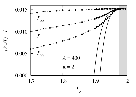
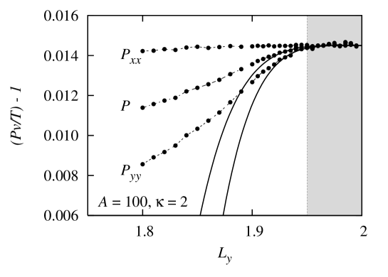
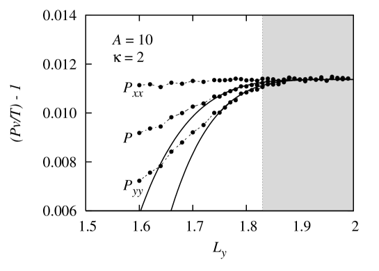
Figure 7: Simulation results for the pressures as a function of the channel width $L_{y}$ with periodic boundaries. The potential parameter $A$ varies from $A=400$ (top) to $A=100$ (middle) and $A=10$ (bottom), and $\kappa=2$. In this figure $N/V=0.01$, and $N=20$. The shaded areas indicate (very conservative) estimates of the scaling regimes. The smooth lines are a fit of Eq. (51) for $P$ and $P_{yy}$ to the data in the shaded regime. Reduced units are used for which $d$ and $E_{0}$ are unity.

The estimated scaling interval, $L_{y,\min}\approx 1.83d<L_{y}<2d$, is indicated by the shaded area. The smooth lines are a fit of Eq. (51) to the numerical data points for $P$ and $P_{yy}$ in that range. It shows that our estimate is rather conservative, since the fits represent the data points reasonably well in a slightly wider interval $1.76d\leq L_{y}\leq 2d$. The kinetic energy per particle is about $0.998E_{0}$ and varies only marginally with $L_{y}$. The scaling is more convincingly demonstrated in Fig. 8, where

Figure 8: Scaling of the transverse pressure $P_{yy}$ for the power-law potential model with $A=10$ and $\kappa=2$ below the critical channel width $L_{y}=2$. Here, $\epsilon=(2-L_{y})$. The slope of the straight line corresponds to the theoretically expected scaling, $\kappa+(1/2)=4.5$. Reduced units are used as explained in the main text.

the $\epsilon$-dependence of the singular part, $\Delta\frac{PV}{\langle K\rangle}\equiv\left[\frac{PV}{\langle K\rangle}\right]-\left[\frac{PV}{\langle K\rangle}\right]_{\epsilon=0}$, for $P_{yy}$ is shown. The straight line indicates the expected scaling with the power 4.5. For $\epsilon>0.07$ corresponding to $L_{y}<1.86\sigma$, the scaling breaks down as expected.

Next, we consider a potential with $A=100E_{0},\;\kappa=2$, which is shown in Fig. 6, and which resembles more realistic repulsive potentials. The channel-width dependence of the pressures is shown in the middle panel of Fig. 7. The estimated scaling range is much narrower than before, $L_{y,\min}=1.95d$, and is indicated by the shaded area. The smooth lines are fits of Eq. (51) to the data points for $P$ and $P_{yy}$ in that interval and confirm that our scaling-range estimate is rather conservative. The kinetic energy per particle is around $0.999E_{0}$ in this case, and varies marginally with $L_{y}$.

Finally, we consider the limiting case of a rather steep potential such as for $A=400E_{0}$ and $\kappa=2$ (much steeper than the $\kappa=2$ curve in Fig. 6), which already resembles that of hard disks and, therefore, should give a pressure variation with $L_{y}$ similar to that found in Ref. FMP04 . The results are shown in the top panel of Fig. 7. The average kinetic energy per particle is $0.9997E_{0}$. For $L_{y}<1.95d$ the pressure curves are indeed very similar to those of a hard-disk gas of 20 disks at the same density and at unit kinetic energy per particle as is shown in Fig. 3 of Ref. FMP04 . Differences appear for channel widths very close to $2d$, which are due to the expected scaling. The estimated scaling range is very narrow, $L_{y,\min}=1.975d$ as indicated by the shaded area in the top panel of Fig. 7. But a fit of Eq. (51) in the range $1.96d\leq L_{y}\leq 2d$ represents the data points for $P$ and $P_{yy}$ reasonably well in that range as is shown by the smooth lines.

Before closing this section, we provide some details about the molecular dynamics simulations. They were carried out with a hybrid code combining the advantages of the event-driven algorithm for hard particles during the forceless streaming stage with the simplicity of a time-stepping integration scheme during the collision of two or more particles. The beginning of each pair collision was determined as in the event-driven algorithms of the previous sections. During the collisions the equations of motion were integrated with a fourth order Runge-Kutta scheme. The end of each pair collision was determined by interpolation with a spatial uncertainty of less than 10^-8 reduced units. The moment the last interacting particles separate, another streaming move is initiated. This method is particularly suited for low densities. It even allows to accurately follow the trajectory for models with discontinuous forces. Periodic boundaries are used. In most cases a trajectory was followed for two million reduced time units $\sqrt{md^{2}/E_{0}}$.

IV Channels with reflecting boundary conditions

IV.1 Soft disks: single step potential

In this section we calculate the pressure components of soft disks in a narrow rectangular box with elastic reflecting boundary conditions in the $y$ direction. Since we are interested in the narrow channel limit where the length of the box is much larger than the width, the system is not sensitive to the boundary conditions in the $x$ direction. For simplicity we take periodic boundary condition in this direction. We consider disks of diameter $d$, which interact with each other via the square well potential of Eq. (13), but with an additional $\delta$-function at the center of the particles:

$$u(r)=\left\{\begin{array}[]{ll}\delta(r)+u&\qquad r\leq d\;,\\ 0&\qquad r>d\;,\end{array}\right.$$ (52)

This $\delta$ function does not affect the particle-particle interactions, but it is responsible for the elastic reflections from the boundary, which confine the disk centers to the volume $V=L_{x}L_{y}$, where $L_{y}$ is referred to as the channel width.

As a result of the reflecting boundary conditions, the system is no longer translationally invariant, and the overlap integral (5) corresponding to the second virial coefficient is replaced by

$$q(L_{y})=\frac{1}{L_{y}}\int f_{12}d^{2}{r_{1}}d^{2}{r_{2}}~{}.$$ (53)

As was done in the case of periodic boundary conditions, with each particle we associate an interaction disk with a radius $d$. Two particles interact with each other only if the center of a particle is within the interaction disk of the other.

In the case $L_{y}>d$ the overlap integral is given by (see the top panel of Fig. 9)

$$q(L_{y})=\frac{1}{L_{y}}\left[\pi d^{2}L_{y}-2\int_{0}^{d}S(\vartheta,d)dy\right](e^{-\beta u}-1)~{},$$ (54)

where $S(\vartheta,d)$ is the segment of a circle of radius $d$ corresponding to a central angle $2\vartheta$,

$$S(\vartheta,d)=d^{2}h(\vartheta)~{},\qquad h(\vartheta)=\vartheta-\sin\vartheta\cos\vartheta~{},\qquad\mbox{and}\qquad\cos\vartheta=\frac{y}{d}~{}.$$ (55)

Evaluating the integral one obtains

$$q(L_{y})=\frac{1}{L_{y}}\left(\pi d^{2}L_{y}-\frac{4}{3}d^{3}\right)(e^{-\beta u}-1)~{}.$$ (56)

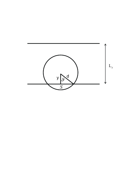
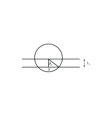
Figure 9: Interaction disks for the square well potential in Eq. (13) for $L_{y}>d$ (top), and $L_{y}<d$ (bottom) in a channel with reflecting boundary condistions.

For $L_{y}<d$ the overlap integral is given by (see the bottom panel of Fig. 9)

$$q(L_{y})=\frac{1}{L_{y}}\left[\pi d^{2}L_{y}-2\int_{0}^{L_{y}}S(\vartheta)dy\right](e^{-\beta u}-1)~{},$$ (57)

where, as in the previous case, $S(\vartheta)$ and $y$ are defined by Eq. (55). The integral can be readily evaluated to yield

$$q(L_{y})=\frac{1}{L_{y}}\left[\pi d^{2}L_{y}-2d^{3}\left(\frac{2}{3}+\vartheta_{0}\cos\vartheta_{0}-\sin\vartheta+\frac{1}{3}\sin^{3}\vartheta_{0}\right)\right](e^{-\beta u}-1)~{},$$ (58)

with

$$\cos\vartheta_{0}=\frac{L_{y}}{d}\;.$$ (59)

The pressure components may be evaluated by using equations (56,58) in the general expressions (7,8).

This analysis demonstrates that the pressure components exhibit a singularity at a channel width $L_{y}=d$. The nature of the singularity is obtained by expanding the overlap integral in $1-L_{y}/d\equiv\epsilon$ for small $\epsilon>0$. In this limit one has $\vartheta_{0}\simeq\sqrt{2\epsilon}$ and $q(L_{y})\simeq-{2/15}\vartheta_{0}^{5}$. Thus, for small $\epsilon$ the singular part of the overlap integral $\delta q(L_{y})$ satisfies

$$\delta q(L_{y})\simeq\epsilon^{5/2}~{}.$$ (60)

As a result, $P_{xx}$ exhibits a $5/2$ singularity at $L_{y}=d$, and its third derivative with respect to $L_{y}$ diverges, as $L_{y}$ approaches $d$ from below. On the other hand, $P_{yy}$ exhibits a stronger, $3/2$, singularity, as it is related to the derivative of the overlap integral with respect to $L_{y}$.

Figure 10: Channel-width dependence of the pressures for $N=60$ particles, which interact with each other with the weak repulsive step potential of Eq. (13), where $u=1$. Reflecting boundary conditions are used as described in the main text. The particle diameter $d=1.5$ in the reduced units applied, and the energy per particle, $E/N$, is unity. Keeping the particle density constant, $N/V=0.01$, the temperature varies slightly with $L_{y}$.

A comparison between theoretical and simulation results is provided in Fig. 10 for a positive step potential. We use reduced units, in which the particle diameter $d$ is 1.5, and for which the total energy per particle, $E/N\equiv E_{0}$, is unity. In these units, we choose for the potential $u=1$. In the simulation we studied $N=120$ particles enclosed in a box with reflecting boundaries both parallel and perpendicular to the channel axis, such that the centers of the particles are confined to the volume $V=L_{x}L_{y}$ (and the particle disks to the volume $(L_{x}+d)(L_{y}+d)$). Varying the channel width $L_{y}$, the density is kept constant, $N/V=0.01$. The singular width, $d$, is indicated by the vertical line. The agreement between the points from the simulation and the theoretical smooth lines corresponding to $P_{xx},P_{yy}$ and $P=(P_{xx}+P_{yy})/2$ is nearly perfect.

To demonstrate the scaling directly, we plot in Fig. 11 the computer simulation results for the singular pressure contributions of $P_{xx}$ and $P_{yy}$ below the singular channel width $L_{y}=d$. To do this, we note that the non-singular contribution to the overlap integral Eq.(58) for $L_{y}<d$ is given by Eq. (56), also evaluated at $L_{y}<d$. The corresponding non-singular (NS) pressure contributions then follow from Eqs. (20) and (21) with $q(L_{y})$ taken from Eq. (56). If this non-singular part is subtracted from the pressures determined by the simulations, a plot of

$$Z_{\alpha\alpha}\equiv\frac{W_{\alpha\alpha}}{\langle K\rangle}-\left[\frac{P_{\alpha\alpha}v}{kT}-1\right]_{\mbox{NS}}\;\;,\alpha\in\{x,y\}$$

as a function of the distance from the singularity, $\epsilon=(d-L_{y})/d$, reveals the expected scaling for the $xx$ and $yy$ pressure components. This is demonstrated by the straight lines in the log-log plot of Fig. 11, which are fully consistent with the expected scaling, 3/2 for $P_{xx}$, and 5/2 for $P_{yy}$.

Figure 11: Channel-width scaling of the singular pressure contributions, which are obtained by subtracting the respective non-singular contributions from the computer simulation results for the pressures (points). The straight lines indicate the theoretically expected scaling. For details we refer to the main text.

It is interesting to note that a system with a purely negative box potential, $u<0$, is thermally unstable and tends to form clusters. The maximum entropy state consists of a single cluster of overlapping disks, floating in the gas of the remaining particles. As a consequence, the specific heat is negative Thirring ; Hertel ; TNP , and the temperature is increased due to the conversion of potential energy into kinetic. Such a property may only arise in the microcanonical ensemble and is familiar for gravitational systems. However, the attracting force need not be of long range PNT90 . A negative specific heat may even be observed for quantum-mechanical Coulomb systems TNP and in experiments on nuclear fragmentation agostino and atomic clusters schmidt ; maerk . In a preliminary study, we have observed the clustering for $u=-1$, but we do not consider this case in more detail, because the times for reaching thermodynamic equilibrium are excessively long.

IV.2 Soft disks with a hard core: two-step potential

In this section we consider particles which interact with a two-step potential

$$u(r)=\left\{\begin{array}[]{ll}\infty&\qquad r\leq d\\ u&\qquad d\leq r<D\\ 0&\qquad r\geq D\end{array}\right.$$ (61)

The soft potential $u$ may be either attractive or repulsive. The disks interact with the walls of the channel only by the hard core interaction with diameter $d$ (In the previous section this potential collapses into a $\delta$ function). As before, we assume reflecting boundary conditions in the $y$ direction as indicated in Figs. 12 and 13, and periodic boundary conditions in the $x$ direction. Thus, the volume accessible to the centers of the particles is given by $V=(L_{y}-d)L_{x}$.

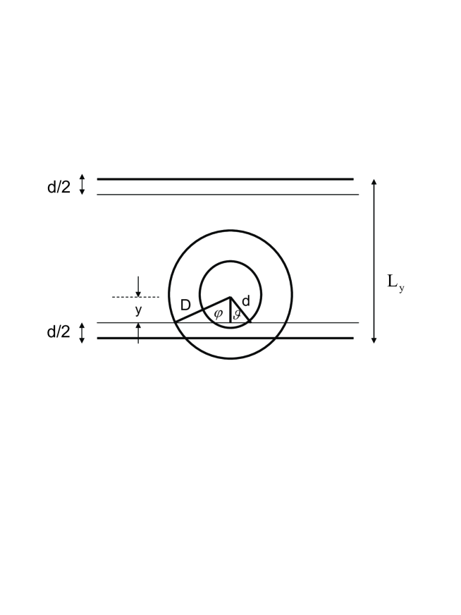
Figure 12: The interaction disks of a particle with a two-step potential in the case of reflecting boundaries. The inner disk is of diameter $2d$ and that of the outer disk is $2D$. The boundaries of the channel are indicated by bold lines. The thin lines, are at a distance $d/2$ from the respective boundary, and they represent the limits, which the centers of the disks cannot cross. The vertical coordinate of the disk, $y$, and the angles $\phi$ and $\vartheta$ are indicated.

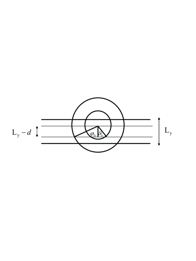
Figure 13: The interaction disks of a particle with a two-step potential in the case of reflecting boundaries for $L_{y}<2d$, where the angles $\phi_{0}$ and $\vartheta_{0}$ are defined. In the intermediate regime $2d<L_{y}<D+d$, the smaller disk does not intersect the boundary of the channel, and $\vartheta_{0}$ becomes $0$.

In calculating the overlap integral, one should distinguish between three regimes.

• For $L_{y}>D+d$ the integral may be expressed as (see Fig. (12))

  $$q(L_{y}) = \pi(D^{2}-d^{2})(e^{-\beta u}-1)-\pi d^{2}$$ (62)

  $$- \frac{2}{L_{y}-d}\left[D^{2}\int_{0}^{D}h(\phi)dy-d^{2}\int_{0}^{d}h(\vartheta)dy\right](e^{-\beta u}-1)$$

  $$+ \frac{2}{L_{y}-d}d^{2}\int_{0}^{d}h(\vartheta)dy~{},$$

  where the function $h$ is given in Eq. (55), and the angles $\phi$ and $\vartheta$ are related to $y$ via (see Fig. (12))

  $$y=d\cos\vartheta=D\cos\phi~{}.$$ (63)

  Evaluating the integrals, one obtains

  $$q(L_{y})=(\pi D^{2}-\frac{4}{3}\frac{D^{3}}{L_{y}-d})(e^{-\beta u}-1)-(\pi d^{2}-\frac{4}{3}\frac{d^{3}}{L_{y}-d})e^{-\beta u}~{}.$$ (64)

• For $2d<L_{y}<D+d$ the overlap integral becomes

  $$q(L_{y}) = \pi(D^{2}-d^{2})(e^{-\beta u}-1)-\pi d^{2}$$ (65)

  $$- \frac{2}{L_{y}-d}\left[D^{2}\int_{0}^{L_{y}-d}h(\phi)dy-d^{2}\int_{0}^{d}h(\vartheta)dy\right](e^{-\beta u}-1)$$

  $$+ \frac{2}{L_{y}-d}d^{2}\int_{0}^{d}h(\vartheta)dy~{}.$$

  The integrals are readily evaluated to yield

  $$q(L_{y}) = (\pi D^{2}-\frac{2D^{3}}{L_{y}-d}g(\phi_{0}))(e^{-\beta u}-1)$$ (66)

  $$- (\pi d^{2}-\frac{4}{3}\frac{d^{3}}{L_{y}-d})e^{-\beta u}~{}.$$

  where

  $$g(\alpha)=\frac{2}{3}+\alpha\cos\alpha-\sin\alpha+\frac{1}{3}\sin^{3}\alpha~{},$$ (67)

  and (see Fig. (13))

  $$\cos\phi_{0}=\frac{L_{y}-d}{D}~{}.$$ (68)

• For $L_{y}<2d$ the overlap integral is

  $$q(L_{y}) = \pi(D^{2}-d^{2})(e^{-\beta u}-1)-\pi d^{2}$$ (69)

  $$- \frac{2}{L_{y}-d}\left[D^{2}\int_{0}^{L_{y}-d}h(\phi)dy-d^{2}\int_{0}^{L_{y}-d}h(\vartheta)dy\right](e^{-\beta u}-1)$$

  $$+ \frac{2}{L_{y}-d}d^{2}\int_{0}^{d}h(\vartheta)dy~{}.$$

  It yields

  $$q(L_{y}) = (\pi D^{2}-\frac{2D^{3}}{L_{y}-d}g(\phi_{0}))(e^{-\beta u}-1)$$ (70)

  $$- (\pi d^{2}-\frac{2D^{3}}{L_{y}-d}g(\vartheta_{0}))e^{-\beta u}~{},$$

  where $\phi_{0}$ is given by Eq. (68), and

  $$\cos\vartheta_{0}=\frac{L_{y}-d}{d}~{},$$ (71)

  (see Fig. (13)).

The nature of the singularities of the pressure components at $L_{y}=D+d$ and $L_{y}=2d$ can be analyzed as before. It is straightforward to show that at both points the $P_{yy}$ components exhibits a $3/2$ singularity, while the $P_{xx}$ component exhibits a $5/2$ singularity.

Figure 14: Channel width dependence of the potential-generated pressures for the interaction potential (61) with $d=1$, $D=1.5$ and $u=1$. The dots are computer simulation results for $N=60$ particles at a density $N/V=0.01$. The smooth lines are obtained from the theoretical overlap integrals of Sec. IV.2. The singular channel widths are indicated by vertical lines. Reduced units are used, for which the particle mass $m$ and the energy per particle, $E/N$, are unity.

Figure 15: Channel width dependence of the potential-generated pressures for the interaction potential (61) with $d=1$, $D=1.5$ and $u=-1$. The dots are computer simulation results for $N=60$ particles at a density $N/V=0.01$. The smooth lines are obtained from the theoretical overlap integrals of Sec. IV.2. The singular channel widths are indicated by vertical lines. Reduced units are used, for which the particle mass $m$ and the energy per particle, $E/N$, are unity.

Comparisons of these results with computer simulations for $N=60$ particles of equal mass $m$ are provided in Fig. 14 for the potential (61) with a positive step $u=1$, and in Fig. 15 for the case of a negative step potential, $u=-1$. All quantities are given in reduced units, for which the particle mass $m$, the hard core diameter, $d$, and the total energy per particle, $E_{0}=E/N$, are unity. The outer diameter is taken to be $D=1.5$. The singular points at $L_{y}=d+D=2.5$ and $L_{y}=2d=2$ are marked by the vertical lines. The density $N/V=0.01$. For the computation of the theoretical pressures resulting in the smooth lines of Figs. 14 and 15, the slight variation of the kinetic energy and, hence, of the temperature with the channel width was taken into account. The agreement between the theoretical expressions and the computer simulation results for the potential part of the pressures is very satisfactory.

V Summary

In the paper we studied the pressure tensor of a system of disks moving in a narrow two dimensional channel, with either periodic or reflecting boundary conditions. We considered the low density regime using the Mayer cluster expansion, and tested the validity of the expansion using molecular dynamics studies. It is found that whenever the two-body interaction potential between disks, $u(r)$, exhibits a singularity at some distance $r_{0}$, the pressure tensor exhibits a singularity as a function of the channel width, at one or more widths which are simply related to $r_{0}$. By studying several classes of interaction potentials, some rather general conclusions regarding the singularities of the pressure tensor can be reached.

In the case of periodic boundary conditions, singularities take place at channel widths $L_{y}=2r_{0}/n$ with $n=1,2,\dots$ . For potentials which exhibit a discontinuity at $r_{0}$, the transverse pressure, $P_{yy}$, exhibits a $1/2$ singularity while the longitudinal component, $P_{xx}$, exhibits a weaker $3/2$ singularity. For potentials which are continuous at $r_{0}$, and whose singular part vanishes as $(r_{0}-r)^{\kappa}$, the transverse pressure exhibits a $2\kappa+1/2$ singularity while the singularity of the longitudinal pressure is $2\kappa+3/2$. Although these results have been demonstrated for specific interaction potentials $u(r)$, they are rather general, as they are related only to the nature of the singularity of the potential.

In the case of reflecting boundary conditions the pressure tensor exhibits a singularity at $L_{y}=r_{0}$. The singularity is weaker than that of the case of periodic boundary conditions. Particularly, it was found that for a potential which is discontinuous at $r_{0}$ , the transverse component of the pressure exhibits a $3/2$ singularity, while the longitudinal component exhibits a weaker $5/2$ singularity.

VI Appendix

There are a few minor misprints in some of the equations in the paper on hard disks FMP04 which are corrected below. These misprints do not affect any of the expressions for the pressure derived in that paper, or any of the numerical results.

In particular, Equation (3) of Ref. FMP04 should read

$$s\equiv\frac{S}{N}=\ln\left(v-\frac{q(L_{y})}{2}\right),$$

and Equation (13) in FMP04 should become

$$\frac{P_{xx}v}{kT} = L_{x}\left(\frac{\partial s}{\partial L_{x}}\right)_{L_{y}},$$

$$\frac{P_{yy}v}{kT} = L_{y}\left(\frac{\partial s}{\partial L_{y}}\right)_{L_{x}}.$$

Another misprint concerns the definition of ${\bf v}_{c}$ in the expression for the virial in Eq. (8). ${\bf v}_{c}$ is the velocity change of a particle $i$ taking part in a binary collision $c$.

VII Acknowledgments

HAP is grateful for the hospitality accorded to him at the Weizmann Institute of Science. Support from the Austrian Science Foundation (FWF), grant P18798, the Minerva Foundation with funding from the Federal German Ministry for Education and Research and the Albert Einstein Minerva Center for Theoretical Physics is gratefully acknowledged. A part of this work was carried out at the Erwin Schrödinger Institute in Vienna on the occasion of a workshop in June 2008.

References

- (1) J. A. Given, J. Chem. Phys. 102, 15 (1995)
- (2) P. M. König, R. Roth and K. R. Mecke, Physa. Rev. Lett. 93, 160601, (2004).
- (3) R. Evans, J. Phys: Condens. Matter. 2, 8989 (1990)
- (4) B. Smit, J. Phys. Chem. 99, 5597 (1995).
- (5) G. Hummer, J. C. Rasaiah and J. P. Nowortya, Nature 414, 188 (2001).
- (6) R. Allen, S. Melchionna and J.-P. Hansen, Phys. Rev. Lett. 89, 175502 (2002).
- (7) B. Hille, Ion Channels of Excitable Membranes, (Sinauer, Sunderland, 2001).
- (8) L. D. Gelb, K. E. Gubbins, R. Radhakrishnan and M. Sliwinska-Bartkowiak, Rep. Prog. Phys. 62, 1573 (1999).
- (9) I. E. Kamenetskiy, K. K. Mon and J. K. Percus, J. Chem. Phys. 121, 7355 (2004).
- (10) H. Kim, E. K. Lee, P. Talkner and P. Hänggi, preprint.
- (11) K. K. Mon and J. K. Percus, J. Chem. Phys. 112, 3457 (2000); J. Chem. Phys. 125, 244704 (2006); J. Chem. Phys. 127, 094702 (2007).
- (12) D. A. Kofke and A. J. Post, J. Chem. Phys. 98, 4853 (1993).
- (13) J. Klafter and J. M. Drake, editors Molecular Dynamics in Restricted Geometries (Wiley, New York, 1989).
- (14) Ch. Forster, D. Mukamel, and H.A. Posch, Phys. Rev. E 69, 066124 (2004). Some minor misprints are corrected in the Appendix of the present paper.
- (15) R. K. Bowles, K. K. Mon and J. K. Percus, J. Chem. Phys. 121, 10668 (2004).
- (16) D. C. Rapaport, The Art of Molecular Dynamics Simulation, Cambridge University Press, 2001, page 296.
- (17) M. P. Allen and D. J. Tildesley, Computer Simulation of Liquids, Oxford University Press, Oxford (1991).
- (18) W. Thirring, Z. Phys. 235, 339 (1970).
- (19) P. Hertel and W. Thirring, Ann. Phys. (N.Y.) 63, 520 (1970).
- (20) W. Thirring, H. Narnhofer, and H.A. Posch, Phys. Rev. Lett. 91, 130601 (2003).
- (21) H. A. Posch, H. Narnhofer, and W. Thirring, Phys. Rev. A 42, 1880 (1090).
- (22) M. D’Agostino, F. Gulminelli, Ph. Chomaz, M. Bruno, F. Cannata, R. Bougault, F. Gramegna, I. Iori, N. Le Neindre, G. V. Margagliotti, A. Moroni, and G. Vannini, Phys. Lett. B 473, 219 (2000).
- (23) M. Schmidt, R. Kusche, T. Hippler. J. Donges, W. Kronmüller, B. von Issendorff, and H. Haberland, Phys. Rev. Lett. 86, 1191 (2001).
- (24) F. Gobet, B. Farizon, M. Farizon, M. J. Gaillard, J. P. Buchet, M. Carré, P. Scheier, and T. D. Märk, Phys. Rev. Lett. 89, 183403 (2002).