Bilateral counterparty risk valuation
with stochastic dynamical models
and application to Credit Default Swaps

Abstract

We introduce the general arbitrage-free valuation framework for counterparty risk adjustments in presence of bilateral default risk, including default of the investor. We illustrate the symmetry in the valuation and show that the adjustment involves a long position in a put option plus a short position in a call option, both with zero strike and written on the residual net value of the contract at the relevant default times. We allow for correlation between the default times of the investor, counterparty and underlying portfolio risk factors. We use arbitrage-free stochastic dynamical models. We then specialize our analysis to Credit Default Swaps (CDS) as underlying portfolio, generalizing the work of Brigo and Chourdakis (2008) [10] who deal with unilateral and asymmetric counterparty risk. We introduce stochastic intensity models and a trivariate copula function on the default times exponential variables to model default dependence. Similarly to [10], we find that both default correlation and credit spread volatilities have a relevant and structured impact on the adjustment. Differently from [10], the two parties will now agree on the credit valuation adjustment. We study a case involving British Airways, Lehman Brothers and Royal Dutch Shell, illustrating the bilateral adjustments in concrete crisis situations.

AMS Classification Codes: 60H10, 60J60, 60J75, 62H20, 91B70
JEL Classification Codes: C15, C63, C65, G12, G13

keywords: Counterparty Risk, Arbitrage-Free Credit Valuation Adjustment, Credit Default Swaps, Contingent Credit Default Swaps, Credit Spread Volatility, Default Correlation, Stochastic Intensity, Copula Functions, Wrong Way Risk.

1 Introduction

General motivation.

In general, the reason to introduce counterparty risk when evaluating a contract is linked to the fact that many financial contracts are traded over the counter, so that the credit quality of the counterparty and of the investor may be important. This has become even more relevant in recent years as some protection sellers such as mono-line insurers or investment banks have witnessed increasing default probabilities or even default events, the case of Lehman Brothers being a clear example.

When investing in default risky assets, one requires a risk premium as a reward for assuming the default risk. If one thinks, for example, of a corporate bond, it is known that the yield is higher than the corresponding yield of an equivalent treasury bond, and this difference is usually called credit spread [12]. The (positive) credit spread implies a lower price for the bond when compared to default free bonds. Many works have been proposed recently to explain the term structure of credit spreads, such as [7], [9], [21], [15] and [2], who also focuses on hedging. This reduction in value is a typical feature: the value of a generic claim traded with a counterparty subject to default risk is always smaller than the value of the same claim traded with a counterparty having a null default probability, as was shown formally for example in [11].

Bilateral risk and symmetry.

This paper introduces a general arbitrage-free valuation framework for bilateral counterparty default risk. By ‘bilateral’ we intend to point out that the default of the investor is included into the framework, contrary to earlier works. This brings about symmetry, so that the price of the position including counterparty risk to the investor is exactly the opposite of the price of the position to the counterparty. This is clearly not the case if each of the two parties computes the present value assuming itself to be default-free and allowing for default of the other party only. This asymmetry would not matter in situations where financial investors had high credit quality and counterparties rather low one. Indeed, in such a case both parties would consider the investor as default-free and the counterparty as defaultable, so that inclusion of the investor default would be pointless, given that it happens in almost no scenario. However, recent events show that it is no longer realistic to take the credit quality of the financial institution for granted and to be highly superior to that of a general counterparty, no matter how prestigious or important the financial institution.

Bilateral risk is also mentioned in the credit risk measurement space by the Basel II documentation, Annex IV, 2/A: “Unlike a firm s exposure to credit risk through a loan, where the exposure to credit risk is unilateral and only the lending bank faces the risk of loss, the counterparty credit risk creates a bilateral risk of loss: the market value of the transaction can be positive or negative to either counterparty to the transaction.”

Basel II is more concerned with Risk Measurement than pricing. For an analysis of Counterparty risk in the risk measurement space we refer for example to De Prisco and Rosen (2005) [20], who consider modeling of stochastic credit exposures for derivatives portfolios. However, also in the valuation space, bilateral features are quite relevant and often can be responsible for seemingly paradoxical statements. For example, Citigroup in its press release on the first quarter revenues of 2009 reported a positive mark to market due to its worsened credit quality: “Revenues also included […] a net 2.5USD billion positive CVA on derivative positions, excluding monolines, mainly due to the widening of Citi s CDS spreads”. In this paper we explain precisely how such a situation may origin.

This paper first generalizes to the bilateral symmetric case the asymmetric unilateral setting proposed in [10], [8], [11] and [13], where only the counterparty is subject to default risk, while the investor is assumed to be default free. We provide a general formula that gives the bilateral risk credit valuation adjustment (BR-CVA) for portfolios exchanged between a default risky investor and a default risky counterparty. Such formula shows that the adjustment to the investor is the difference between two discounted options terms, a discounted call option in scenarios of early default time of the counterparty minus a discounted put option in scenarios of early default times of the investor, both options being on the residual net present value of the portfolio at the relevant default times and having zero strike. The BR-CVA seen from the point of view of the counterparty is exactly the opposite. We allow for correlation between default of the investor, default of the counterparty and underlying portfolio risk factors, and for volatilities and dynamics in the credit spreads and in the underlying portfolio, all arbitrage free.

Bilateral Counterparty adjustment applied to CDS.

We then specialize our analysis to Credit Default Swaps (CDS) as underlying portfolio, generalizing the work of Brigo and Chourdakis [10] who deal with unilateral and asymmetric counterparty risk for these contracts. Featuring a CDS as underlying, a third default time enters the picture, namely the default time for the reference credit of the CDS. We therefore assume that all three entities are subject to default risk and that the default events of investor, counterparty and reference credit are correlated. We then propose a numerical methodology to evaluate the resulting BR-CVA formula. We investigate the impact of both credit spread volatility and default correlation on the credit valuation adjustment. Most of previous approaches on CDS counterparty risk only focus on unilateral counterparty risk, moreover ignoring the effect of volatility on the adjustment and mainly focusing on default correlation.

The few earlier works on CDS with counterparty risk include Leung and Kwok (2005)[24] who, building on Collin-Dufresne et al. (2002) [16], model default intensities as deterministic constants with default indicators of other names as feeds. The exponential triggers of the default times are taken to be independent and default correlation results from the cross feeds, although again there is no explicit modeling of credit spread volatility. Hull and White [23] study the counterparty risk problem by resorting to barrier correlated models. Walker (2005) [30] models CDS counterparty risk using transitions rates as natural means to represent contagion, but again ignores credit spread volatility. Hille et al. (2006)[22] concentrate on credit risk measurement for CDS rather than precise valuation under counterparty risk.

The need for explicitly modeling credit spread volatility is even more pronounced if the underlying reference contract is itself a CDS, as the credit valuation adjustment would involve CDS options and it is very undesirable to model options without volatility in the underlying asset. This has been clearly shown in [10] for CDS, and in [13] for interest rates payoffs, and again in [8] for commodities payoffs. Indeed, most credit models in the industry, especially when applied to Collateralized Debt Obligations or $k$-th to default baskets, model default correlation but ignore credit spread volatility. Credit spreads are typically assumed to be deterministic and a copula is postulated on the exponential triggers of the default times to model default correlation. This is the opposite of what used to happen with counterparty risk for interest rate underlyings, for example in Sorensen and Bollier (1994) [28] or Brigo and Masetti [11] (in Pykhtin (2006)[27]), where correlation was ignored and volatility was modeled instead. Brigo and Chourdakis (2008) [10] rectify this when addressing CDS’s, but only deal with unilateral and asymmetric counterparty risk.

Summarizing, we can put this paper’s contribution into context with respect to its analogous earlier versions for unilateral counterparty risk or for other asset classes through Table 1.

Other recent works include Crépey et al (2009)[19] who model wrong way risk for CDS with counterparty risk using a Markov chain copula model, and Blanchet-Scalliet and Patras (2008) [3], who resort to older Merton type models. A structural model with jumps has been introduced by Lipton and Sepp (2009) [25]. In these models assumptions on credit spread volatility are most time implicit.

Here instead we introduce stochastic intensity models for all three names, including the investor. We do not introduce correlation between the three intensity processes, but model default correlation through a trivariate copula function on the exponential triggers of the default times. This is because typically spread correlation has a much lower impact on dependence of default times than default correlation. The correlation structure underlying the trivariate copula function may be estimated by the implied correlation in the quoted indices tranches markets such as i-Traxx and CDX or calculated from the asset correlation of the names. We leave this problem for further research. We present a preliminary numerical investigation to highlight the impact of dynamics parameters on bilateral CVA, followed by a case study of bilateral risk based on British Airways, Lehman Brothers and Royal Dutch Shell. We confirm findings in [10] showing that both default correlation and credit spread volatilities have a relevant and structured impact on the adjustment.

We specify that we do not consider specific collateral clauses or guarantees in the present work. We assume we are dealing with counterparty risk for an over the counter CDS transaction where there is no periodic margining or collateral posting. The aim of this paper is analyzing the fine structure of counterparty risk adjustments with respect to finely tuned market dynamics, including the fundamental credit spread volatility ignored in other approaches, and wrong way risk. We plan to address collateral provisions inclusion in future work. We already addressed netting in the interest rate context in [13] and [11]. The impact of credit triggers for the counterparty on CVA are analyzed in Yi (2009) [29]. Assefa et al (2009) [1] analyze the modeling of collateralization and margining in CVA calculations.

Modeling $\rightarrow$	Underlying Volatility	Underlying Vol +	Bilateral
Asset Class $\downarrow$	No underl/counterp Corr	underl/counterp Corr	+ Vol and Corr
IR swaps	(Net) B. Masetti [11]	(Net) B. Pallavicini [13]	(Net) Brigo Pallavicini
			& Papatheodorou [14]
			(forthcoming)
IR exotics		B. Pallavicini [13]	B. P. P. [14]
			(forthcoming)
Oil swaps		B. Bakkar [8]
CDS		B. Chourdakis [10]	This paper
Equity		B. Masetti [11]

Table 1: Part of earlier analogous literature on CVA valuation with respect to inclusion of volatilities and correlation and of bilateral features. “Net” denotes papers that consider netting.

Paper structure.

The rest of the paper is organized as follows. Section 2 gives the general BR-CVA formula and refers to the appendix for the mathematical proof. Section 3 defines the underlying framework needed for applying the above methodology to credit default swaps, including the stochastic intensity model and the trivariate copula function for correlating defaults. Section 4 develops a numerical method to implement the formula in the case when the underlying contract is a CDS and gives the pseudo code of the algorithm used to run numerical simulations. Section 5 present numerical experiments on different default correlation scenarios and changes in credit spread volatility. Section 6 presents a specific application for computing the mark-to-market value of a CDS contract agreed between British Airways, Lehman Brothers and Royal Shell. Section 7 concludes the paper.

2 Arbitrage-free valuation of bilateral counterparty risk

We refer to the two names involved in the financial contract and subject to default risk as

investor $$\rightarrow$$ name “0”

counterparty $$\rightarrow$$ name “2”

In cases where the portfolio exchanged by the two parties is also a default sensitive instrument, we introduce a third name referring to the reference credit of that portfolio

$$\text{reference credit }\rightarrow\text{name ``1''}$$

If the portfolio is not default sensitive then name “1” can be removed.

We follow [6] and denote by $\tau_{0}$, ($\tau_{1}$) and $\tau_{2}$ respectively the default times of the investor, (reference credit) and counterparty. We place ourselves in a probability space $(\Omega,\mathcal{G},\mathcal{G}_{t},\mathbb{Q})$. The filtration $\mathcal{G}_{t}$ models the flow of information of the whole market, including credit and $\mathbb{Q}$ is the risk neutral measure. This space is endowed also with a right-continuous and complete sub-filtration $\mathcal{F}_{t}$ representing all the observable market quantities but the default event, thus $\mathcal{F}_{t}\subseteq\mathcal{G}_{t}:=\mathcal{F}_{t}\vee\mathcal{H}_{t}$. Here, $\mathcal{H}_{t}=\sigma(\{\tau_{0}\leq u\}(\vee\{\tau_{1}\leq u\})\vee\{\tau_{2}\leq u\}:u\leq t)$ is the right-continuous filtration generated by the default events, either of the investor or of his counterparty (and of the reference credit if the underlying portfolio is credit sensitive). We also introduce the notion of stopped filtration. If $\tau$ is an $\mathcal{F}_{t}$ stopping time, then the stopped filtration $\mathcal{F}_{\tau}$ is defined as

$$\mathcal{F}_{\tau}=\sigma(\mathcal{F}_{t}\cup\{t\leq\tau\},t\geq 0)$$ (2.1)

If $\tau$ is an $\mathcal{G}_{t}$ stopping time, then the stopped filtration $\mathcal{G}_{\tau}$ is defined as

$$\mathcal{G}_{\tau}=\sigma(\mathcal{G}_{t}\cup\{t\leq\tau\},t\geq 0)$$ (2.2)

Let us call $T$ the final maturity of the payoff which we need to evaluate and let us define the stopping time

$$\tau=\min\{\tau_{0},\tau_{2}\}$$ (2.3)

If $\tau>T$, there is neither default of the investor, nor of his counterparty during the life of the contract and they both can fulfill the agreements of the contract. On the contrary, if $\tau\leq T$ then either the investor or his counterparty (or both) defaults. At $\tau$, the Net Present Value (NPV) of the residual payoff until maturity is computed. We then distinguish two cases:

• $\tau=\tau_{2}$. If the NPV is negative (respectively positive) for the investor (defaulted counterparty), it is completely paid (received) by the investor (defaulted counterparty) itself. If the NPV is positive (negative) for the investor (counterparty), only a recovery fraction REC,2 of the NPV is exchanged.

• $\tau=\tau_{0}$. If the NPV is positive (respectively negative) for the defaulted investor (counterparty), it is completely received (paid) by the defaulted investor (counterparty) itself. If the NPV is negative (positive) for the defaulted investor (counterparty), only a recovery fraction REC,0 of the NPV is exchanged.

Let us define the following (mutually exclusive and exhaustive) events ordering the default times

$$A = \{\tau_{0}\leq\tau_{2}\leq T\}\ \ \ \ \ E=\{T\leq\tau_{0}\leq\tau_{2}\}$$

$$B = \{\tau_{0}\leq T\leq\tau_{2}\}\ \ \ \ \ F=\{T\leq\tau_{2}\leq\tau_{0}\}$$

$$C = \{\tau_{2}\leq\tau_{0}\leq T\}$$

$$D = \{\tau_{2}\leq T\leq\tau_{0}\}$$ (2.4)

Let us call $\Pi^{D}(t,T)$ the discounted payoff of a generic defaultable claim at $t$ and $\mbox{C{\tiny ASHFLOWS}}(u,s)$ the net cash flows of the claim without default between time $u$ and time $s$, discounted back at $u$, all payoffs seen from the point of view of the investor. Then, we have $\mbox{NPV}(\tau_{i})=\mathbb{E}_{\tau_{i}}\{\mbox{C{\tiny ASHFLOWS}}(\tau_{i},T)\}$, $i=0,2$. Let us denote by $D(t,T)$ the price of a zero coupon bond with maturity $T$. We have

$$\Pi^{D}(t,T) = \mathbf{1}_{E\cup F}\mbox{C{\tiny ASHFLOWS}}(t,T)$$

$$+\mathbf{1}_{C\cup D}\left[\mbox{C{\tiny ASHFLOWS}}(t,\tau_{2})+D(t,\tau_{2})\left(\mbox{R{\tiny EC,2}}\left(\mbox{NPV}(\tau_{2})\right)^{+}-\left(-\mbox{NPV}(\tau_{2})\right)^{+}\right)\right]$$

$$+\mathbf{1}_{A\cup B}\left[\mbox{C{\tiny ASHFLOWS}}(t,\tau_{0})+D(t,\tau_{0})\left(\left(\mbox{NPV}(\tau_{0})\right)^{+}-\mbox{R{\tiny EC,0}}\left(-\mbox{NPV}(\tau_{0})\right)^{+}\right)\right]$$

This last expression is the general payoff under bilateral counterparty default risk. Indeed, if there is no early default, this expression reduces to risk neutral valuation of the payoff (first term on the right hand side). In case of early default of the counterparty, the payments due before default occurs are received (second term), and then if the residual net present value is positive only the recovery value of the counterparty REC,2 is received (third term), whereas if it is negative it is paid in full by the investor (fourth term). In case of early default of the investor, the payments due before default occurs are received (fifth term), and then if the residual net present value is positive it is paid in full by the counterparty to the investor (sixth term), whereas if it is negative only the recovery value of the investor REC,0 is paid to the counterparty (seventh term).

Let us denote by $\Pi(t,T)$ the discounted payoff for an equivalent claim with a default-free counterparty, i.e. $\Pi(t,T)=\mbox{C{\tiny ASHFLOWS}}(t,T)$. We then have the following

Proposition 2.1 ([6]).

(General bilateral counterparty risk pricing formula). At valuation time $t$, and conditional on the event $\{\tau>t\}$, the price of the payoff under bilateral counterparty risk is

$$\mathbb{E}_{t}\left\{\Pi^{D}(t,T)\right\} = \mathbb{E}_{t}\left\{\Pi(t,T)\right\}$$ (2.6)

$$+\mathbb{E}_{t}\left\{\mathrm{LGD}_{0}\cdot\mathbf{1}_{A\cup B}\cdot D(t,\tau_{0})\cdot\left[-\mathrm{NPV}(\tau_{0})\right]^{+}\right\}$$

$$-\mathbb{E}_{t}\left\{\mathrm{LGD}_{2}\cdot\mathbf{1}_{C\cup D}\cdot D(t,\tau_{2})\cdot\left[\mathrm{NPV}(\tau_{2})\right]^{+}\right\}$$

where $LGD=1-\mbox{R{\tiny EC}}$ is the Loss Given Default and the recovery fraction REC can be stochastic and possibly correlated with the default indicator process. It is clear that the value of a defaultable claim is the value of the corresponding default-free claim plus a long position in a put option (with zero strike) on the residual NPV giving nonzero contribution only in scenarios where the investor is the earliest to default (and does so before final maturity) plus a short position in a call option (with zero strike) on the residual NPV giving nonzero contribution in scenarios where the counterparty is the earliest to default (and does so before final maturity),

Proposition 2.1 is stated in [6] without a proof. Here, we provide a mathematical proof in Appendix A. The adjustment is called bilateral counterparty risk credit valuation adjustment (BR-CVA) and it may be either positive or negative depending on whether the counterparty is more or less likely to default than the investor and on the volatilities and correlation. The mathematical expression is given by

$$\mathrm{BR\text{-}CVA}(t,T,\mathrm{LGD}_{0,1,2}) = \mathbb{E}_{t}\left\{\mathrm{LGD}_{2}\cdot\mathbf{1}_{C\cup D}\cdot D(t,\tau_{2})\cdot\left[\mathrm{NPV}(\tau_{2})\right]^{+}\right\}$$ (2.7)

$$-\mathbb{E}_{t}\left\{\mathrm{LGD}_{0}\cdot\mathbf{1}_{A\cup B}\cdot D(t,\tau_{0})\cdot\left[-\mathrm{NPV}(\tau_{0})\right]^{+}\right\}$$

where the right hand side in Eq. (2.7) depends on $T$ through the events $A,B,C,D$ and $\mathrm{LGD}_{012}=(\mathrm{LGD}_{0},\mathrm{LGD}_{1},\mathrm{LGD}_{2})$ is shorthand notation to denote the dependence on the loss given defaults of the three names.

Remark 2.2.

(Symmetry vs Asymmetry). With respect to earlier results on counterparty risk valuation, Equation (2.7) has the great advantage of being symmetric. This is to say that if “2” were to compute counterparty risk of her position towards “1”, she would find exactly $-\mathrm{BR\text{-}CVA}(t,T,\mathrm{LGD}_{0,1,2})$. However, if each party computed the adjustment by assuming itself to be default-free and considering only the default of the other party, then the adjustment calculated by “0” would be

$$\mathbb{E}_{t}\left\{\mathrm{LGD}_{2}\cdot\mathbf{1}_{\tau_{2}<T}\cdot D(t,\tau_{2})\cdot\left[\mathrm{NPV}(\tau_{2})\right]^{+}\right\}$$

whereas the adjustment calculated by “2” would be

$$\mathbb{E}_{t}\left\{\mathrm{LGD}_{0}\cdot\mathbf{1}_{\tau_{0}<T}\cdot D(t,\tau_{0})\cdot\left[-\mathrm{NPV}(\tau_{0})\right]^{+}\right\}$$

and they would not be one the opposite of the other. This means that only in the first case the two parties agree on the value of the counterparty risk adjustment.

Remark 2.3.

(Change in sign). Earlier results on counterparty risk valuation, concerned with a default-free investor and asymmetric, would find an adjustment to be subtracted that is always positive. However, in our symmetric case even if the initial adjustment is positive due to

$$\mathbb{E}_{t}\left\{\mathrm{LGD}_{2}\cdot\mathbf{1}_{C\cup D}\cdot D(t,\tau_{2})\cdot\left[\mathrm{NPV}(\tau_{2})\right]^{+}\right\}>\mathbb{E}_{t}\left\{\mathrm{LGD}_{0}\cdot\mathbf{1}_{A\cup B}\cdot D(t,\tau_{0})\cdot\left[-\mathrm{NPV}(\tau_{0})\right]^{+}\right\}$$

the situation may change in time, to the point that the two terms may cancel or that the adjustment may change sign as the credit quality of “0” deteriorates and that of “2” improves, so that the inequality changes direction.

Remark 2.4.

(Worsening of credit quality and positive mark to market). If the Investor marks to market her position at a later time using Formula (2.6), we can see that the term in $\mbox{L{\tiny GD}}_{0}$ increases, ceteris paribus, if the credit quality of “0” worsens. Indeed, if we increase the credit spreads of the investor, now $\tau_{0}<\tau_{2}$ will happen more often, giving more weight to the term in $\mbox{L{\tiny GD}}_{0}$. This is at the basis of statements like the above one of Citigroup.

3 Application to Credit Default Swaps

In this section we use the formula developed in Section 2 to evaluate the BR-CVA in credit default swap contracts (CDS). Subsection 3.1 recalls the general formula for CDS evaluation. Subsection 3.2 introduces the copula models used to correlate the default events. Subsection 3.3 recalls the CIR model used for the stochastic intensity of the three names. Subsection 3.4 applies the general BR-CVA formula to calculate the adjustment for CDS contracts. We restrict our attention to CDS contract without an upfront trading. However, the proposed methodology is perfectly applicable to the case when the CDS trades with an upfront premium, which has become the case after the big bang protocol.

3.1 CDS Payoff

We assume deterministic interest rates, which leads to independence between $\tau_{1}$ and $D(0,t)$, and deterministic recovery rates. Our results hold also true for the case of stochastic rates independent of default times. The receiver CDS valuation, for a CDS selling protection LGD₁ at time 0 for default of the reference entity between times $T_{a}$ and $T_{b}$ in exchange of a periodic premium rate $S_{1}$ is given by

$$\mbox{CDS}_{a,b}(0,S_{1},\mathrm{LGD}_{1}) = S_{1}\bigg{[}-\int_{T_{a}}^{T_{b}}D(0,t)(t-T_{\gamma(t)-1})d\mathbb{Q}(\tau_{1}>t)$$ (3.1)

$$+\sum_{i=a+1}^{b}\alpha_{i}D(0,T_{i})\mathbb{Q}(\tau_{1}>T_{i})\bigg{]}$$

$$+\mathrm{LGD}_{1}\left[\int_{T_{a}}^{T_{b}}D(0,t)d\mathbb{Q}(\tau_{1}>t)\right]$$

where $\gamma(t)$ is the first payment period $T_{j}$ following time $t$. Let us denote by

$$\mbox{NPV}(T_{j},T_{b}):=\mbox{CDS}_{a,b}(T_{j},S,\mathrm{LGD}_{1})$$ (3.2)

the residual NPV of a receiver CDS between $T_{a}$ and $T_{b}$ evaluated at time $T_{j}$, with $T_{a}<T_{j}<T_{b}$. Eq. (3.2) can be written similarly to Eq. (3.1), except that now evaluation occurs at time $T_{j}$ and has to be conditioned on the information set available to the market at $T_{j}$. This leads to

$$\mbox{CDS}_{a,b}(T_{j},S_{1},\mathrm{LGD}_{1}) = \mathbf{1}_{\tau_{1}>T_{j}}\overline{\mbox{CDS}}_{a,b}(T_{j},S_{1},LGD_{1})$$ (3.3)

$$:= \mathbf{1}_{\tau_{1}>T_{j}}\bigg{\{}S_{1}\bigg{[}-\int^{T_{b}}_{\max\{T_{a},T_{j}\}}D(T_{j},t)(t-T_{\gamma(t)-1})d\mathbb{Q}(\tau_{1}>t|\mathcal{G}_{T_{j}})$$

$$+\sum_{i=\max\{a,j\}+1}^{b}\alpha_{i}D(T_{j},T_{i})\mathbb{Q}(\tau_{1}>T_{i}|\mathcal{G}_{T_{j}})\bigg{]}$$

$$+\mathrm{LGD}_{1}\bigg{[}\int^{T_{b}}_{\max\{T_{a},T_{j}\}}D(T_{j},t)d\mathbb{Q}(\tau_{1}>t|\mathcal{G}_{T_{j}})\bigg{]}\bigg{\}}$$

For conversion of these running CDS into upfront ones, following the so called Big Bang protocol by ISDA, see for example Beumee, Brigo, Schiemert and Stoyle (2009)[4]. Our reasoning still applies with obvious modifications to the upfront CDS contract.

3.2 Default Correlation

We consider a reduced form model that is stochastic in the default intensity for the investor, counterparty and CDS reference credit. The default correlation between the three names is defined through a dependence structure on the exponential random variables characterizing the default times of the three names. Such dependence structure is modeled using a trivariate copula function. Let us denote by $\lambda_{i}(t)$ and $\Lambda_{i}(t)=\int_{0}^{t}\lambda_{i}(s)ds$ respectively the default intensity and cumulated intensity of name $i$ evaluated at time $t$. We recall that $i=0$ refers to the investor, $i=1$ refers to the reference credit and $i=2$ to the counterparty. We assume $\lambda_{i}$ to be independent of $\lambda_{j}$ for $i\neq j$, and assume each of them to be strictly positive almost everywhere, thus implying that $\Lambda_{i}$ is invertible. We stress the fact that independence of $\lambda$’s across names does not mean that the default event of one name does not change the default probability or intensity of other names, as discussed in [10], Section 4. We place ourselves in a Cox process setting, where

$$\tau_{i}=\Lambda_{i}^{-1}(\xi_{i}),\ i=0,1,2$$ (3.4)

with $\xi_{0}$, $\xi_{1}$ and $\xi_{2}$ being standard (unit-mean) exponential random variables whose associated uniforms

$$U_{i}=1-\exp\{-\xi_{i}\}$$ (3.5)

are correlated through a Gaussian trivariate copula function

$$C_{\bm{R}}(u_{0},u_{1},u_{2})=\mathbb{Q}(U_{0}<u_{0},U_{1}<u_{1},U_{2}<u_{2})$$ (3.6)

with $\bm{R}=[r_{i,j}]_{i,j=0,1,2}$ being the correlation matrix parameterizing the Gaussian copula. Notice that a trivariate Gaussian copula implies bivariate Gaussian marginal copulas. We show it for the case of the bivariate copula connecting the reference credit and the counterparty, but the same argument applies to the other bivariate copulas. Let $(X_{1},X_{2},X_{3})$ be a standard Gaussian vector with correlation matrix $\bm{R}$ and let $\Phi_{\bm{R}}$ be the distribution function of a multivariate Gaussian random variable with correlation matrix $\bm{R}$. For any pair of indices $i\neq j$, $0\leq i,j\leq 2$, we denote by $\bm{R}_{i,j}$ the $2\cdot 2$ submatrix formed by the intersection of row $i$ and row $j$ with column $i$ and column $j$. We next state, without proof, an obvious result as a Lemma, which will be later used.

Lemma 3.1.

A trivariate Gaussian copula with correlation matrix $\bm{R}$ induces marginal bivariate Gaussian copulas.

We denote by $C_{i,j}(u_{i},u_{j})$ the bivariate copula associated to $\bm{R}_{i,j}$.

3.3 CIR stochastic intensity model

We assume the following stochastic intensity model [7], [9] for the three names

$$\lambda_{j}(t)=y_{j}(t)+\psi_{j}(t;\bm{\beta}_{j}),\ t\geq 0,j=0,1,2$$ (3.7)

where $\psi$ is a deterministic function, depending on the parameter vector $\bm{\beta}$ (which includes $y_{0}$), that is integrable on closed intervals. We assume each $y_{j}$ to be a Cox Ingersoll Ross (CIR) process [12] given by

$$dy_{j}(t)=\kappa_{j}(\mu_{j}-y_{j}(t))dt+\nu_{j}\sqrt{y_{j}(t)}dZ_{j}(t)+J_{M_{t},j}dM_{j}(t),j=0,1,2$$ (3.8)

where $J$’s are i.i.d. positive jump sizes that are exponentially distributed with mean $\chi_{j}$ and $M_{j}$ are Poisson processes with intensity $m_{j}$ measuring the arrival of jumps in the intensity $\lambda_{j}$. The parameter vectors are $\bm{\beta}_{j}=(\kappa_{j},\mu_{j},\nu_{j},y_{j}(0),\chi_{j},m_{j})$ with each vector component being a positive deterministic constant. We relax the condition of inaccessibility of the origin $2\kappa_{j}\mu_{j}>\nu_{j}^{2}$ so that we do not limit the CDS implied volatility generated by the model. We assume the $Z_{j}$’s to be standard Brownian motion processes under the risk neutral measure. We define the following integrated quantities which will be extensively used in the remainder of the paper

$$\Lambda_{j}(t)=\int_{0}^{t}\lambda_{j}(s)ds,\ \ Y_{j}(t)=\int_{0}^{t}y_{j}(s)ds,\ \ \Psi_{j}(t;\bm{\beta}_{j})=\int_{0}^{t}\psi_{j}(s;\bm{\beta}_{j})ds$$ (3.9)

In this paper, we focus on intensities without jumps, i.e. $m_{j}=0$. Brigo and El-Bachir [9] consider in detail the tractable model with jumps, and this extension will be applied in future work.

3.4 Bilateral risk credit valuation adjustment for receiver CDS

We next proceed to the valuation of the BR-CVA adjustment for the case of CDS payoff given by Eq. (3.1). We state the result as a Proposition.

Proposition 3.2.

The $\mathrm{BR\text{-}CVA}$ at time $t$ for a receiver CDS contract (protection seller) running from time $T_{a}$ to time $T_{b}$ with premium $S$ is given by

$$\mathrm{BR\text{-}CVA\text{-}CDS}_{a,b}(t,S,\mathrm{LGD}_{0,1,2}) = \mathrm{LGD}_{2}\cdot\mathbb{E}_{t}\left\{\mathbf{1}_{C\cup D}\cdot D(t,\tau_{2})\cdot\left[\mathbf{1}_{\tau_{1}>\tau_{2}}\overline{\mbox{CDS}}_{a,b}(\tau_{2},S,LGD_{1})\right]^{+}\right\}$$

$$-\mathrm{LGD}_{0}\cdot\mathbb{E}_{t}\left\{\mathbf{1}_{A\cup B}\cdot D(t,\tau_{0})\cdot\left[-\mathbf{1}_{\tau_{1}>\tau_{0}}\overline{\mbox{CDS}}_{a,b}(\tau_{0},S,LGD_{1})\right]^{+}\right\}$$

Proof.

We have

$$\mathbb{E}_{t}\left\{\mathbf{1}_{C\cup D}\cdot D(t,\tau_{2})\cdot\left[\mathrm{NPV}(\tau_{2})\right]^{+}\right\} = \mathbb{E}_{t}\left\{\mathbf{1}_{C\cup D}\cdot D(t,\tau_{2})\cdot\left[\mbox{CDS}_{a,b}(\tau_{2},S,\mathrm{LGD}_{1})\right]^{+}\right\}$$

$$= \mathbb{E}_{t}\left\{\mathbf{1}_{C\cup D}\cdot D(t,\tau_{2})\cdot\left[\mathbf{1}_{\tau_{1}>\tau_{2}}\overline{\mbox{CDS}}_{a,b}(\tau_{2},S,\mathrm{LGD}_{1})\right]^{+}\right\}$$

where the first equality in Eq. (LABEL:eq:cds_counterparty_developed) follows by definition, while the last equality follows from Eq. (3.3). Similarly, we have

$$\mathbb{E}_{t}\left\{\mathbf{1}_{A\cup B}\cdot D(t,\tau_{0})\cdot\left[-\mathrm{NPV}(\tau_{0})\right]^{+}\right\} = \mathbb{E}_{t}\left\{\mathbf{1}_{A\cup B}\cdot D(t,\tau_{0})\cdot\left[-\mbox{CDS}_{a,b}(\tau_{0},S,\mathrm{LGD}_{1})\right]^{+}\right\}$$

$$= \mathbb{E}_{t}\left\{\mathbf{1}_{A\cup B}\cdot D(t,\tau_{0})\cdot\left[-\mathbf{1}_{\tau_{1}>\tau_{0}}\overline{\mbox{CDS}}_{a,b}(\tau_{0},S,\mathrm{LGD}_{1})\right]^{+}\right\}$$

The proof follows using the expression of BR-CVA which is given by Eq. (2.7). ∎

To summarize, in order to compute the counterparty risk adjustment, we determine the value of the CDS contract on the reference credit “1” at the point in time $\tau_{2}$ at which the counterparty “2” defaults. The reference name “1” has survived this point and there is a bivariate copula $C_{1,2}$ which connects the default times of the reference credit and of the counterparty “2”. Similarly, in order to compute the investor risk adjustment, we determine the value of the CDS contract on the reference credit “1” at the point in time $\tau_{0}$ at which the counterparty “0” defaults. The reference name “1” has survived this point and there is a bivariate copula $C_{0,1}$ which connects the default times of the reference credit and of the investor “0”. It is clear from Eq. (3.3) and Eq. (2.7) that the only terms we need to know in order to compute (LABEL:eq:cds_counterparty_developed) and (LABEL:eq:cds_investor_developed) are

$$\mathbf{1}_{C\cup D}\mathbf{1}_{\tau_{1}>\tau_{2}}\mathbb{Q}(\tau_{1}>t|\mathcal{G}_{\tau_{2}})$$ (3.13)

and

$$\mathbf{1}_{A\cup B}\mathbf{1}_{\tau_{1}>\tau_{0}}\mathbb{Q}(\tau_{1}>t|\mathcal{G}_{\tau_{0}})$$ (3.14)

In the next section, we generalize the numerical method proposed in [10] to calculate quantities (3.13) and (3.14) for the bilateral counterparty case.

4 Monte-Carlo Evaluation of the BR-CVA adjustment

We propose a numerical method based on Monte-Carlo simulations to calculate the BR-CVA for the case of CDS contracts. Subsection 4.1 specifies the simulation method used to generate the sample paths of the CIR process. Subsection 4.2 gives a method to calculate (3.13), while Subsection 4.3 gives the complete numerical algorithm for calculating the BR-CVA in (LABEL:eq:biladj).

4.1 Simulation of CIR process

We use the well known fact [12] that the distribution of $y(t)$ given $y(u)$, for some $u<t$ is, up to a scale factor, a noncentral chi-square distribution. More precisely, the transition law of $y(t)$ given $y(u)$ can be expressed as

$$y(t)=\frac{\nu^{2}(1-e^{-\kappa(t-u)})}{4\kappa}\chi^{\prime}_{d}\left(\frac{4\kappa e^{-\kappa(t-u)}}{\nu^{2}(1-e^{-\kappa(t-u)})}y(u)\right)$$ (4.1)

where

$$d=\frac{4\kappa\mu}{\nu^{2}}$$ (4.2)

and $\chi^{\prime}_{u}(v)$ denotes a non-central chi-square random variable with $u$ degrees of freedom and non centrality parameter $v$. In this way, if we know $y(0)$, we can simulate the process $y(t)$ exactly on a discrete time grid by sampling from the non-central chi-square distribution.

4.2 Calculation of Survival Probability

We state the result in the form of a proposition. Such result will be used in Subsection 4.3 to develop a numerical algorithm for computing the BR-CVA. Let us define

$$\overline{U}_{i,j}=1-\exp(-\Lambda_{i}(\tau_{j}))$$ (4.3)

and denote by $F_{\Lambda_{i}(t)}$ the cumulative distribution function of the cumulative (shifted) intensity of the CIR process associated to name $i$, which can be retrieved inverting the characteristic function of the integrated CIR process. We have

Proposition 4.1.

$$\mathbf{1}_{C\cup D}\mathbf{1}_{\tau_{1}>\tau_{2}}\mathbb{Q}(\tau_{1}>t|\mathcal{G}_{\tau_{2}})=$$

$$\mathbf{1}_{\tau_{2}\leq T}\mathbf{1}_{\tau_{2}\leq\tau_{0}}\left(\mathbf{1}_{\bar{A}}+\mathbf{1}_{\tau_{2}<t}\mathbf{1}_{\tau_{1}\geq\tau_{2}}\int_{\overline{U}_{1,2}}^{1}F_{\Lambda_{1}(t)-\Lambda_{1}(\tau_{2})}(-\log(1-u_{1})-\Lambda_{1}(\tau_{2}))dC_{1|0,2}(u_{1};U_{2})\right)$$

(4.4)

where

$$\bar{A} = \{t<\tau_{2}<\tau_{1}\}$$

$$C_{1|0,2}(u_{1};U_{2}) = \frac{\frac{\partial C_{1,2}(u_{1},u_{2})}{\partial u_{2}}\bigg{|}_{u_{2}=U_{2}}-\frac{\partial C(\overline{U}_{0,2},u_{1},u_{2})}{\partial u_{2}}\bigg{|}_{u_{2}=U_{2}}-\frac{\partial C_{1,2}(\overline{U}_{1,2},u_{2})}{\partial u_{2}}\bigg{|}_{u_{2}=U_{2}}+\frac{\partial C(\overline{U}_{0,2},\overline{U}_{1,2},u_{2})}{\partial u_{2}}\bigg{|}_{u_{2}=U_{2}}}{1-\frac{\partial C_{0,2}(\overline{U}_{0,2},u_{2})}{\partial u_{2}}\bigg{|}_{u_{2}=U_{2}}-\frac{\partial C_{1,2}(\overline{U}_{1,2},u_{2})}{\partial u_{2}}\bigg{|}_{u_{2}=U_{2}}+\frac{\partial C(\overline{U}_{0,2},\overline{U}_{1,2},u_{2})}{\partial u_{2}}\bigg{|}_{u_{2}=U_{2}}}$$

Similarly,

Proposition 4.2.

$$\mathbf{1}_{A\cup B}\mathbf{1}_{\tau_{1}>\tau_{0}}\mathbb{Q}(\tau_{1}>t|\mathcal{G}_{\tau_{0}})=$$

$$\mathbf{1}_{\tau_{0}\leq T}\mathbf{1}_{\tau_{0}\leq\tau_{2}}\left(\mathbf{1}_{\bar{B}}+\mathbf{1}_{\tau_{0}<t}\mathbf{1}_{\tau_{1}\geq\tau_{0}}\int_{\overline{U}_{1,0}}^{1}F_{\Lambda_{1}(t)-\Lambda_{1}(\tau_{0})}(-\log(1-u_{1})-\Lambda_{1}(\tau_{0}))dC_{1|2,0}(u_{1};U_{0})\right)$$

(4.6)

where

$$\bar{B} = \{t<\tau_{0}<\tau_{1}\}$$

$$C_{1|2,0}(u_{1};U_{0}) = \frac{\frac{\partial C_{0,1}(u_{0},u_{1})}{\partial u_{0}}\bigg{|}_{u_{0}=U_{0}}-\frac{\partial C(u_{0},u_{1},\overline{U}_{2,0})}{\partial u_{0}}\bigg{|}_{u_{0}=U_{0}}-\frac{\partial C_{0,1}(u_{0},\overline{U}_{1,0})}{\partial u_{0}}\bigg{|}_{u_{0}=U_{0}}+\frac{\partial C(u_{0},\overline{U}_{1,0},\overline{U}_{2,0})}{\partial u_{0}}\bigg{|}_{u_{0}=U_{0}}}{1-\frac{\partial C_{0,2}(u_{0},\overline{U}_{2,0})}{\partial u_{0}}\bigg{|}_{u_{0}=U_{0}}-\frac{\partial C_{0,1}(u_{0},\overline{U}_{1,0})}{\partial u_{0}}\bigg{|}_{u_{0}=U_{0}}+\frac{\partial C(u_{0},\overline{U}_{1,0},\overline{U}_{2,0})}{\partial u_{0}}\bigg{|}_{u_{0}=U_{0}}}$$

The proofs of the propositions are reported in Appendix B.

4.3 The numerical BR-CVA adjustment algorithm

We give the pseudo code of the numerical algorithm used to calculate the BR-CVA for the CDS payer and receiver. In the pseudo-code below, the variable $\alpha_{i}$ represents the time elapsing between payment period $t_{i-1}$ and $t_{i}$ measured in years, the variable $\Delta$ represents the fineness of the grid used to evaluate the integral of the survival probability in Eq. (4.4) and the variable $\delta$ represents the fineness of the time grid used to evaluate the integral in Eq. (3.3). The variable $x_{\max}$ represents the maximum $x$ value for which the cumulative distribution function is implied from the characteristic function. The expression CDF($x_{k}$) corresponds to a subroutine call which calculates the cumulative distribution function of the integrated CIR process at $x_{k}$. This can be done by inversion of the characteristic function of the integrated CIR process using Fourier transform methods such as in [18]. The inputs to the main procedure Calculate Adjustment are the number $N$ of Monte-Carlo runs and the market quote $S_{1}$ of the 5 year CDS spread of the reference entity.

Algorithm 1 $[\overline{\text{BR-CVA\_R}},\overline{\text{BR-CVA\_P}}]$ = Calculate Adjustment (N, S)

  for $i=1:N$ do

     Generate $\tau_{0}$, $\tau_{1}$, and $\tau_{2}$ using Eq. (3.5) and Eq. (3.6).

     if $\tau_{2}<\tau_{0}$ and $\tau_{2}<T_{b}$ then

        if $\tau_{1}>\tau_{2}$ then

           $[$BR-CVA_R_2, BR-CVA_P_2$]$ = CDSAdjust($T_{\gamma(\tau_{2})}$, $S$, $\mathrm{LGD}_{1}$, 2)

           CUM_BR-CVA_R = CUM_BR-CVA_R + $\mathrm{LGD}_{2}\cdot$ BR-CVA_R_2

           CUM_BR-CVA_P = CUM_BR-CVA_P + $\mathrm{LGD}_{2}\cdot$ BR-CVA_P_2

        end if

     end if

     if $\tau_{0}<\tau_{2}$ and $\tau_{0}<T_{b}$ then

        if $\tau_{1}>\tau_{0}$ then

           $[$BR-CVA_R_0, BR-CVA_P_0$]$ = CDSAdjust($T_{\gamma(\tau_{0})}$, $S$, $\mathrm{LGD}_{1}$, 0)

           CUM_BR-CVA_R = CUM_BR-CVA_R - $\mathrm{LGD}_{0}\cdot$ BR-CVA_R_0

           CUM_BR-CVA_P = CUM_BR-CVA_P - $\mathrm{LGD}_{0}\cdot$ BR-CVA_P_0

        end if

     end if

  end for

  $\overline{\text{BR-CVA\_R}}$ = CUM_BR-CVA_R / $N$

  $\overline{\text{BR-CVA\_P}}$ = CUM_BR-CVA_P / $N$

Algorithm 2 [$CDS_{R},CDS_{P}$] = CDSAdjust($T_{j},S$, $\mathrm{LGD}_{1}$, $index$)

  $Term_{1}=Term_{2}=Term_{3}=0$

  $t_{start}=\max(T_{a},T_{j})$

  $Q_{prev}=$ ComputeProb($t_{start}$, $T_{j}$, $index$)

  for $t=t_{start}+\delta:\delta:T_{b}$ do

     $Q_{curr}=$ ComputeProb($t,T_{j},index$)

     $Term_{1}=Term_{1}+D(T_{j},t-\delta)(t-\delta-T_{\gamma(t-\delta)-1})(Q_{curr}-Q_{prev})$

     $Term_{3}=Term_{3}+D(T_{j},t-\delta)(Q_{curr}-Q_{prev})$

     $Q_{prev}=Q_{curr}$

  end for

  for $t_{i}=t_{start}+\alpha_{i}:\alpha_{i}:T_{b}$ do

     $Q_{curr}=$ ComputeProb($t_{i},T_{j},index$)

     $Term_{2}=Term_{2}+\alpha_{i}\cdot D(T_{j},t_{i})\cdot Q_{curr}$

  end for

  $CDS_{val}=S\cdot(Term_{2}-Term_{1})$ + $\mathrm{LGD}_{1}\cdot Term_{3}$

  if $index==2$ then

     $CDS_{R}=D(t,T_{j})\cdot\max(CDS_{val},0)$

     $CDS_{P}=D(t,T_{j})\cdot\max(-CDS_{val},0)$

  end if

  if $index==0$ then

     $CDS_{R}=D(t,T_{j})\cdot\max(-CDS_{val},0)$

     $CDS_{P}=D(t,T_{j})\cdot\max(CDS_{val},0)$

  end if

Algorithm 3 $Q_{i}$ = ComputeProb($t,T_{j},index$)

  $U_{index}=1-\exp\{-Y_{index}(T_{j})-\Psi_{index}(T_{j};\bm{\beta}_{index})\}$

  $\bar{U}_{1}=1-\exp\{-Y_{1}(T_{j})-\Psi_{1}(T_{j};\bm{\beta}_{1})\}$

  for $x_{k}=0:\Delta:x_{\max}$ do

     $p_{k}$ = CDF($x_{k}$)

     $u_{k}=1-\exp\{-x_{k}-\Psi_{1}(t)\}$

     if index == 2 then

        Compute $f_{k}=C_{1|0,2}(u_{k};U_{2})$ using Eq. (LABEL:eq:copula2first)

     else

        Compute $f_{k}=C_{1|2,0}(u_{k};U_{0})$ using Eq. (LABEL:eq:copula0first)

     end if

  end for

  $Q_{i}=\sum_{(u_{k},p_{k},f_{k}):u_{k}>\bar{U}_{1}}p_{k}(f_{k+1}-f_{k})$

5 Numerical Results

We consider an investor (name “0”) trading a five-years CDS contract on a reference name (name “1”) with a counterparty (name “2”). Both the investor and the counterparty are subject to default risk. We experiment on different levels of credit risk and credit risk volatility of the three names, which are specified by the parameters of the CIR processes in Table 2.

Credit Risk Levels	$y(0)$	$\kappa$	$\mu$	Credit Risk volatilities	$\nu$
low	0.00001	0.9	0.0001	low	0.01
middle	0.01	0.80	0.02	middle	0.2
high	0.03	0.50	0.05	high	0.5

Table 2: The credit risk levels and credit risk volatilities parameterizing the CIR processes

We recall that the survival probabilities associated with a CIR intensity process are given by

$$\mathbb{Q}(\tau_{i}>t) := \mathbb{E}[e^{-Y_{i}(t)}]$$ (5.1)

$$= P^{CIR}(0,t,\bm{\beta}_{i})$$

where $P^{CIR}(0,t,\bm{\beta}_{i})$ is the price at time 0 of a zero coupon bond maturing at time $t$ under a stochastic interest rate dynamics given by the CIR process [12], with $\bm{\beta}_{i}=(y_{i}(0),\kappa_{i},\mu_{i},\nu_{i})$ being the vector of CIR parameters, $i=0,1,2$.

We report in Table 3 the break-even spreads zeroing (3.1) in $S$, with survival probabilities given by Eq. (5.1) and CIR parameters $\bm{\beta}_{low}$, $\bm{\beta}_{middle}$, $\bm{\beta}_{high}$ obtained from Table 2.

Maturity	Low Risk	Middle Risk	High risk
1y	0	92	234
2y	0	104	244
3y	0	112	248
4y	1	117	250
5y	1	120	251
6y	1	122	252
7y	1	124	253
8y	1	125	253
9y	1	126	254
10y	1	127	254

Table 3: Break-even spreads in basis points generated using the parameters of the CIR processes in Table 2. The first column is generated using low credit risk and credit risk volatility. The second column is generated using middle credit risk and credit risk volatility. The third column is generated using high credit risk and credit risk volatility.

The evaluation time $t$ and the starting time $T_{a}$ of the CDS contract are both set to zero. The end time $T_{b}$ of the contract is set to five years. It is assumed that payments are exchanged every three months. The loss given defaults of the low, middle and high risk entity are respectively set to $\mathrm{LGD}_{low}=0.6$, $\mathrm{LGD}_{middle}=0.65$, $\mathrm{LGD}_{high}=0.7$. We assume that the spreads in Table 3 are the spreads quoted in the markets for the three names under consideration. We recover the integrated shift $\Psi(t;\bm{\beta})$ which makes the model survival probabilities consistent with the market survival probabilities coming from Table 3 whenever we change the CIR parameters. In mathematical terms, for any $i=0,1,2$, we impose that

$$\mathbb{Q}(\tau_{i}>t)_{model} := \mathbb{E}[e^{-\Lambda_{i}(t)}]$$ (5.2)

$$= \mathbb{Q}(\tau_{i}>t)_{market}$$

The market survival probability for name “$i$” is bootstrapped from the market CDS quotes reported in Table 3. Such bootstrap procedure is performed assuming a piecewise linear hazard rate function. From the definition of the integrated process $\Psi_{j}(t;\bm{\beta}_{j})$ given in Eq. (3.9), we can restate Eq. (5.2) as

$$\Psi_{i}(t;\bm{\beta}_{i}) = \log\left(\frac{\mathbb{E}[e^{-Y_{i}(t)}]}{\mathbb{Q}(\tau_{i}>t)_{market}}\right)$$ (5.3)

$$= \log\left(\frac{P^{CIR}(0,t,\bm{\beta}_{i})}{\mathbb{Q}(\tau_{i}>t)_{market}}\right)$$

where the last equality in Eq. (5.3) follows from Eq. (5.1). We first study a case where the quoted market spreads of the investor has a low credit risk profile ($\beta_{low}$), the reference entity has high credit risk profile ($\beta_{high}$), while the counterparty has middle credit risk ($\beta_{middle}$). We vary the correlation between reference credit and counterparty as well as the credit risk volatility $\nu_{1}$ of the reference credit. Since the focus is mostly on credit spreads volatility, we calculate the implied CDS volatility produced by the choice of parameters $\bm{\beta}_{1}=(y_{0}(1),\mu_{1},\kappa_{1},\nu_{1})$ for a hypothetical CDS option, maturing in one year and in case of exercise entering into a four year CDS contract on the underlying reference credit “1”. The objective of the experiments is to measure the impact of correlation and credit spreads volatility on the BR-CVA. The triple $(x,y,z)$ represents the correlation of the trivariate Gaussian copula, with $x$ denoting the correlation between the investor and reference credit, $y$ denoting the correlation between the investor and the counterparty and $z$ denoting the correlation between the reference credit and the counterparty. The values $\overline{\text{BR-CVA\_P}}$ and $\overline{\text{BR-CVA\_R}}$ are respectively the Monte-Carlo estimates of the CDS payer and receiver counterparty risk adjustments. The theoretical formula for payer risk adjustment is given by

$$\mathrm{\mathrm{LGD}_{2}\cdot\mathbb{E}_{t}\left\{\mathbf{1}_{C\cup D}\cdot D(t,\tau_{2})\cdot\left[-\mathrm{NPV}(\tau_{2})\right]^{+}\right\}}$$

$$-\mathrm{\mathrm{LGD}_{0}\cdot\mathbb{E}_{t}\left\{\mathbf{1}_{A\cup B}\cdot D(t,\tau_{0})\cdot\left[\mathrm{NPV}(\tau_{0})\right]^{+}\right\}}$$ (5.4)

which follows from adapting the formula given in Eq. (LABEL:eq:biladj), given for the receiver counterparty adjustment, to the case of the payer counterparty adjustment. Tables 4 and 5 report the results obtained.

$(r_{01},r_{02},r_{12})$	Vol. parameter $\nu_{1}$	0.01	0.10	0.20	0.30	0.40	0.50
	CDS Impled vol	1.5%	15%	28%	37%	42%	42%
(0, 0, -0.99)	$\overline{\text{BR-CVA\_P}}$	0.0(0.0)	0.0(0.0)	0.0(0.0)	0.0(0.0)	-0.0(0.0)	-0.0(0.0)
	$\overline{\text{BR-CVA\_R}}$	29.3(1.5)	29.7(1.5)	29.8(1.5)	29.8(1.5)	29.8(1.5)	29.6(1.5)
(0, 0, -0.90)	$\overline{\text{BR-CVA\_P}}$	0.0(0.0)	0.0(0.0)	0.0(0.0)	0.0(0.0)	-0.0(0.0)	-0.0(0.0)
	$\overline{\text{BR-CVA\_R}}$	29.6(1.5)	29.2(1.5)	29.1(1.5)	29.3(1.5)	29.6(1.5)	29.0(1.5)
(0, 0, -0.60)	$\overline{\text{BR-CVA\_P}}$	0.0(0.0)	0.0(0.0)	0.0(0.0)	0.1(0.0)	0.4(0.2)	0.6(0.2)
	$\overline{\text{BR-CVA\_R}}$	27.0(1.4)	27.2(1.4)	26.4(1.4)	26.6(1.4)	25.4(1.3)	25.2(1.3)
(0, 0, -0.20)	$\overline{\text{BR-CVA\_P}}$	0.0(0.0)	0.4(0.1)	1.3(0.2)	2.0(0.3)	2.6(0.4)	3.2(0.5)
	$\overline{\text{BR-CVA\_R}}$	10.3(0.7)	10.4(0.7)	10.9(0.7)	12.1(0.7)	12.8(0.8)	13.0(0.8)
(0, 0, 0)	$\overline{\text{BR-CVA\_P}}$	4.8(0.3)	5.1(0.4)	5.4(0.5)	7.4(0.8)	5.9(0.6)	5.6(0.7)
	$\overline{\text{BR-CVA\_R}}$	0.0(0.0)	0.5(0.1)	2.1(0.2)	3.9(0.3)	5.0(0.3)	6.3(0.4)
(0, 0, 0.20)	$\overline{\text{BR-CVA\_P}}$	25.9(1.5)	25.1(1.5)	23.2(1.5)	21.1(1.6)	15.9(1.3)	12.8(1.2)
	$\overline{\text{BR-CVA\_R}}$	0.0(0.0)	0.0(0.0)	0.2(0.0)	0.5(0.1)	0.7(0.1)	1.1(0.1)
(0, 0, 0.60)	$\overline{\text{BR-CVA\_P}}$	72.0(4.9)	72.0(4.8)	65.2(4.4)	57.1(4.0)	50.8(3.6)	40.4(3.0)
	$\overline{\text{BR-CVA\_R}}$	0.0(0.0)	0.0(0.0)	0.0(0.0)	0.0(0.0)	0.0(0.0)	0.1(0.0)
(0, 0, 0.90)	$\overline{\text{BR-CVA\_P}}$	68.4(6.1)	73.8(6.3)	69.2(5.8)	65.2(5.4)	61.5(5.0)	62.2(4.9)
	$\overline{\text{BR-CVA\_R}}$	0.0(0.0)	0.0(0.0)	0.0(0.0)	0.0(0.0)	0.0(0.0)	0.0(0.0)
(0, 0, 0.99)	$\overline{\text{BR-CVA\_P}}$	13.2(2.8)	28.4(4.0)	39.4(4.4)	51.9(4.9)	54.8(5.0)	67.6(5.4)
	$\overline{\text{BR-CVA\_R}}$	0.0(0.0)	0.0(0.0)	0.1(0.0)	0.1(0.0)	0.1(0.0)	0.4(0.3)

Table 4: BR-CVA in basis points for the case when $y_{0}(0)=0.0001,\kappa_{0}=0.01,\mu_{0}=0.001,\nu_{0}=0.01$, $y_{0}(2)=0.01,\kappa_{2}=0.8,\mu_{2}=0.02,\nu_{2}=0.2$. The name “1” has CIR parameters $y_{0}(1)=0.03,\kappa_{1}=0.5,\mu_{1}=0.05$, while the credit spreads volatility $\nu_{1}$ is varied across scenarios. The numbers within round brackets represent the Monte-Carlo standard error. The CDS contract on the reference credit has a five-years maturity.

$(r_{01},r_{02},r_{12})$	Vol. parameter $\nu_{1}$	0.01	0.10	0.20	0.30	0.40	0.50
	CDS Impled vol	1.5%	15%	28%	37%	42%	42%
(0, 0, -0.99)	$\overline{\text{BR-CVA\_P}}$	0.0(0.0)	0.0(0.0)	0.0(0.0)	0.0(0.0)	0.0(0.0)	0.0(0.0)
	$\overline{\text{BR-CVA\_R}}$	28.8(1.4)	29.2(1.4)	28.3(1.4)	28.0(1.4)	29.3(1.4)	28.9(1.4)
(0, 0, -0.90)	$\overline{\text{BR-CVA\_P}}$	0.0(0.0)	0.0(0.0)	0.0(0.0)	0.0(0.0)	0.1(0.0)	0.1(0.0)
	$\overline{\text{BR-CVA\_R}}$	28.9(1.4)	29.0(1.4)	28.2(1.4)	28.7(1.4)	28.8(1.4)	28.9(1.4)
(0, 0, -0.60)	$\overline{\text{BR-CVA\_P}}$	0.0(0.0)	0.0(0.0)	0.1(0.1)	0.1(0.0)	0.8(0.2)	0.2(0.1)
	$\overline{\text{BR-CVA\_R}}$	26.8(1.3)	26.5(1.3)	25.7(1.3)	25.1(1.3)	24.9(1.3)	25.0(1.3)
(0, 0, -0.20)	$\overline{\text{BR-CVA\_P}}$	0.0(0.0)	0.4(0.1)	1.3(0.2)	2.4(0.4)	2.8(0.5)	2.0(0.4)
	$\overline{\text{BR-CVA\_R}}$	9.7(0.6)	9.7(0.6)	10.4(0.7)	11.7(0.7)	12.7(0.7)	13.0(0.7)
(0, 0, 0)	$\overline{\text{BR-CVA\_P}}$	4.8(0.2)	5.3(0.4)	6.0(0.5)	6.6(0.7)	5.2(0.7)	5.1(0.7)
	$\overline{\text{BR-CVA\_R}}$	0.0(0.0)	0.5(0.1)	2.1(0.2)	3.8(0.3)	5.0(0.3)	6.0(0.3)
(0, 0, 0.20)	$\overline{\text{BR-CVA\_P}}$	26.6(1.5)	26.1(1.5)	23.6(1.5)	19.7(1.4)	16.7(1.4)	13.8(1.4)
	$\overline{\text{BR-CVA\_R}}$	0.0(0.0)	0.0(0.0)	0.1(0.0)	0.4(0.0)	0.7(0.1)	1.0(0.1)
(0, 0, 0.60)	$\overline{\text{BR-CVA\_P}}$	76.4(4.8)	74.1(4.6)	68.1(4.4)	60.8(4.0)	52.2(3.7)	42.3(3.1)
	$\overline{\text{BR-CVA\_R}}$	0.0(0.0)	0.0(0.0)	0.0(0.0)	0.0(0.0)	0.1(0.0)	0.1(0.0)
(0, 0, 0.90)	$\overline{\text{BR-CVA\_P}}$	75.3(6.1)	76.1(6.1)	74.4(5.9)	68.8(5.5)	62.2(5.2)	64.4(4.9)
	$\overline{\text{BR-CVA\_R}}$	0.0(0.0)	0.0(0.0)	0.0(0.0)	0.0(0.0)	0.0(0.0)	0.0(0.0)
(0, 0, 0.99)	$\overline{\text{BR-CVA\_P}}$	12.6(2.6)	24.9(3.6)	41.3(4.5)	51.8(4.9)	55.3(4.9)	65.9(5.3)
	$\overline{\text{BR-CVA\_R}}$	0.0(0.0)	0.0(0.0)	0.1(0.0)	0.1(0.0)	0.1(0.0)	0.1(0.0)

Table 5: BR-CVA in basis points for the case when $y_{0}(0)=0.0001,\kappa_{0}=0.01,\mu_{0}=0.001,\nu_{0}=0.01$, $y_{0}(2)=0.01,\kappa_{2}=0.8,\mu_{2}=0.02,\nu_{2}=0.01$. The name “1” has CIR parameters $y_{0}(1)=0.03,\kappa_{1}=0.5,\mu_{1}=0.05$, while the credit spreads volatility $\nu_{1}$ is varied across scenarios. The numbers within round brackets represent the Monte-Carlo standard error. The CDS contract on the reference credit has a five-years maturity.

The scenarios considered in Table 4 and 5 assume an investor with an extremely low credit risk profile and thus are similar to those considered in [10], where the investor is assumed to be default-free. Therefore, it is not surprising that we find similar results. Similarly to them, we can see that the BR-CVA for the payer investor tends to be monotonically increasing with the correlation $r_{12}$, whereas the BR-CVA for the receiver investor appears to be monotonically decreasing. This is expected since for low and negative correlation values, defaults of the counterparty come with reductions in default risk of the reference entity, thus the receiver investor holds an option which is in the money, but at the counterparty default he only gets a fraction of it proportional to the recovery value of the counterparty. On the contrary, for high and positive correlation values, defaults of the counterparty come with increases in default risk of the reference entity, thus the payer investor holds an option which is in the money, but at the counterparty default he only gets a fraction of it proportional to the recovery value of the counterparty. While these patterns are intuitive, there is a particular pattern in correlation that is seemingly counterintuitive.

Remark 5.1.

(Decreasing wrong way risk with low credit spread volatility and high correlation). In general, we expect the BR-CVA for the payer investor to increase with correlation between the underlying reference credit and the counterparty default. However, for correlation increasing beyond relatively large values, the BR-CVA for the payer investor goes down instead, if the credit spreads volatility of the reference entity is small. Consider, for example, the case when the reference entity and the counterparty are $99\%$ correlated, so that the exponential triggers $\xi_{1}$ and $\xi_{2}$ are almost identical. If we consider the scenario where $\nu_{1}=\nu_{2}=0.01$, then the intensity of both processes are almost deterministic, with $\lambda_{1}>\lambda_{2}$ having the name “1” high credit risk and name “2” middle credit risk. Thus, to a first approximation $\tau_{1}=\frac{\xi_{1}}{\lambda_{1}}$ is higher than $\tau_{2}=\frac{\xi_{2}}{\lambda_{2}}$, and consequently the reference credit always defaults before the counterparty, resulting in no adjustment. Table 5 has qualitatively a similar behavior. This is visible also in the right side of the graphs in the upper Figure 1, where the pattern goes down at the very end for correlations beyond 0.9.

This seemingly counterintuitive feature is improved if credit spread volatility becomes large (and in line with realistic CDS implied volatilities, see Brigo (2005)[5]). This is evident from the last column of Table 5, and is due to the increased randomness in the default times, that now can cross each other in more scenarios.

To further illustrate the transition from large (small) to small (large) adjustments for the receiver (payer) investor and illustrate the effect of correlation and credit spreads volatility, we display in Figure 1 the behavior of the bilateral risk adjustment for two different values of credit spreads volatility.

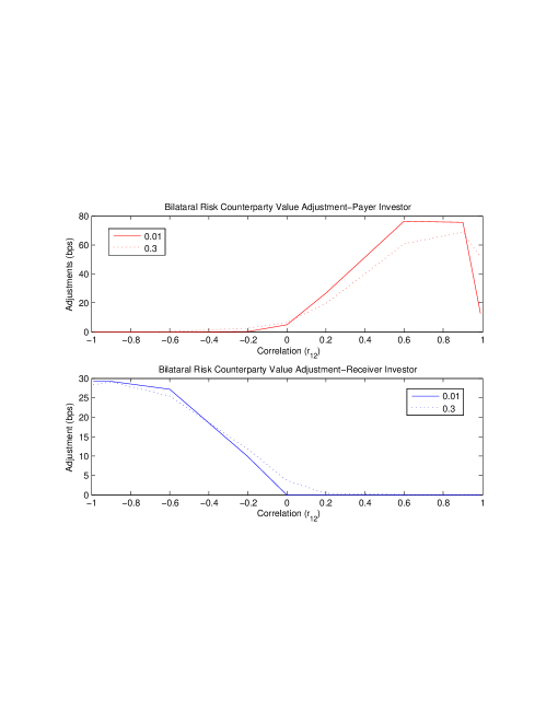
Figure 1: Patterns of the $\overline{\text{BR-CVA}}$ of the CDS contract for payer and receiver investor and for low (0.1) and high (0.3) reference credit spreads volatility $\nu_{1}$. We have that $\nu_{2}=0.01$ and $\nu_{0}=0.01$

Tables 6 and 7 report the BR-CVA adjustments for the Payer CDS under a set of five different riskiness scenarios. The assignments of credit risks in Table 2 to the three names determine the scenario in place. We have:

• Scenario 1 (Base Scenario). The investor has low credit risk, the reference entity has high credit risk, and the counterparty has middle credit risk

• Scenario 2 (Risky counterparty). The investor has low credit risk, the reference entity has middle credit risk, and the counterparty has high credit risk.

• Scenario 3 (Risky investor). The counterparty has low credit risk, the reference entity has middle credit risk, and the investor has high credit risk.

• Scenario 4 (Risky Ref). Both investor and counterparty have middle credit risk, while the reference entity has high credit risk.

• Scenario 5 (Safe Ref). Both investor and counterparty have high credit risk, while the reference entity has low credit risk.

$(r_{01},r_{02},r_{12})$	Base Scenario	Risky Counterparty	Risky Investor	Risky Ref	Safe Ref
(0, 0, 0)	6.0(0.4)	3.6(0.2)	-0.8(0.0)	-0.0(0.0)	5.5(0.4)
(0, 0, 0.1)	15.1(0.8)	12.6(0.5)	-0.8(0.0)	-0.0(0.0)	13.2(1.0)
(0, 0, 0.3)	37.0(2.0)	37.4(1.5)	-0.8(0.1)	0.1(0.0)	34.6(2.1)
(0, 0, 0.6)	73.7(4.4)	92.5(3.8)	-0.3(0.5)	0.7(0.1)	67.3(4.3)
(0, 0, 0.9)	83.4(6.0)	207.8(8.2)	-0.8(0.0)	1.5(0.3)	75.7(5.8)
(0, 0, 0.99)	26.0(3.5)	316.9(12.5)	-0.8(0.0)	1.8(0.5)	22.6(3.4)
(0, 0.1, 0)	6.0(0.4)	3.6(0.2)	-0.8(0.0)	-0.0(0.0)	4.2(0.3)
(0, 0.3, 0)	5.8(0.4)	3.6(0.2)	-0.8(0.0)	-0.0(0.0)	3.7(0.3)
(0, 0.6, 0)	6.0(0.4)	3.6(0.2)	-0.8(0.1)	-0.0(0.0)	5.9(0.4)
(0, 0.9, 0)	0.6(4.5)	3.5(0.2)	-0.8(0.0)	0.0(0.0)	15.0(1.5)
(0.1, 0, 0)	6.0(0.4)	3.6(0.2)	-0.1(0.0)	-0.0(0.0)	6.5(0.4)
(0.3, 0, 0)	6.0(0.4)	3.6(0.2)	0.0(0.0)	0.0(0.0)	6.6(0.4)
(0.6, 0, 0)	6.0(0.4)	3.6(0.2)	0.0(0.0)	0.0(0.0)	6.5(0.4)
(0.9, 0, 0)	5.9(0.4)	3.6(0.2)	0.0(0.0)	-0.1(0.0)	6.6(0.4)
(0.99, 0, 0)	5.9(0.4)	3.6(0.2)	-1.8(0.1)	-0.1(0.0)	6.7(0.4)

Table 6: BR-CVA under five different riskiness scenarios. The CIR volatilities are set to $\nu_{0}=\nu_{1}=\nu_{2}=0.1$. The correlation triple has two non-zero entries

$(r_{01},r_{02},r_{20})$	Base Scenario	Risky Counterparty	Risky Investor	Risky Ref	Safe Ref
(0.7, 0.4, 0.3)	37.0(2.1)	36.4(1.4)	-0.0(0.0)	-0.0(0.0)	8.4(0.7)
(0.7, 0.3, 0.4)	49.0(2.8)	51.4(2.1)	0.1(0.1)	0.2(0.0)	25.8(1.7)
(0.4, 0.7, 0.3)	35.3(2.0)	35.5(1.4)	0.1(0.1)	0.1(0.0)	27.0(1.7)
(0.4, 0.3, 0.7)	79.8(5.0)	117.4(4.9)	0.6(0.5)	0.6(0.1)	74.0(4.9)
(0.3, 0.4, 0.7)	80.8(5.1)	117.8(4.9)	0.0(0.0)	0.6(0.1)	73.6(5.5)
(0.3, 0.7, 0.4)	45.8(2.7)	50.0(2.0)	0.0(0.0)	0.4(0.0)	50.9(3.3)
(0.3, 0.3, 0.3)	36.4(2.0)	36.7(1.4)	0.0(0.0)	0.1(0.0)	28.2(1.7)
(0.4, 0.4, 0.4)	47.9(2.8)	50.8(2.1)	0.0(0.0)	0.2(0.0)	39.0(2.4)
(0.7, 0.7, 0.7)	77.4(5.0)	113.6(4.8)	0.0(0.0)	0.6(0.1)	82.5(6.5)

Table 7: BR-CVA under five different riskiness scenarios. The CIR volatilities are set to $\nu_{0}=\nu_{1}=\nu_{2}=0.1$. The correlation triple has all non-zero entries

Tables 6 and 7 clearly show the effect of the wrong way risk. For example, looking at the second column, we can see that as the correlation between counterparty and reference entity gets larger, the BR-CVA increases significantly. This is because (1) the counterparty is the riskiest name and (2) the high positive correlation makes the spread of the reference entity larger at the counterparty default, thus the option on the residual NPV for the payer investor will be deep into the money and worth more. If the only correlation is between reference credit and counterparty, then the adjustment is the largest, while when the counterparty is less correlated with the reference entity, but also positively correlated with the investor (see second column of Table 7), then the adjustment tends to decrease as the number of scenarios where the counterparty is the earliest to default is smaller.

The first six rows of Table 6 show how much the BR-CVA adjustment is driven by correlation and credit spreads volatility. When the counterparty and reference entity are loosely correlated, then the adjustments in Scenario 1 and Scenario 2 are very similar, although the counterparty is riskier in Scenario 2. However, as the correlation increases, the BR-CVA adjustment in Scenario 2 becomes significantly larger than the corresponding adjustment in Scenario 1. Differently from Tables 4 and 5, however, we have that low credit risk volatility values has the opposite effect and amplify the adjustment; this is because for 99% correlation between reference credit and counterparty, we now have that the counterparty always defaults earlier being riskier.

Consistently with the results in Table 4 and 5, no BR-CVA takes place in scenario 4. This is because the reference entity has the highest credit risk profile and since the credit risk volatilities of the three names are relatively low, the reference entity always defaults first, thus resulting in no adjustment taking place.

6 Application to a market scenario

We apply the methodology to calculate the mark-to-market price of a five-year CDS contract between British Airways (counterparty) and Lehman Brothers (investor) on the default of Royal Dutch Shell (reference credit). We consider two CDS contracts. In the first contract Lehman Brothers buys 5-year protection on Shell from British Airways on January 5, 2006. In the second contract, Lehman Brothers sells 5-year protection on Shell to British Airways on January 5, 2006. In both contracts, British Airways computes the mark-to-market value of the contract on May 1, 2008. We consider different correlation scenarios among the three names. The CDS quotes of the three names on those dates are reported in Tables 8 and 9.

Maturity	Royal Dutch Shell	Lehman Brothers	British Airways
1y	4	6.8	10
2y	5.8	10.2	23.2
3y	7.8	14.4	50.6
4y	10.1	18.7	80.2
5y	11.7	23.2	110
6y	15.8	27.3.3	129.5
7y	19.4	30.5	142.8
8y	20.5	33.7	153.6
9y	21	36.5	162.1
10y	21.4	38.6	168.8

Table 8: Market spread quotes in basis points for Royal Dutch Shell, Lehman Brothers and British Airways on January 5, 2006.

Maturity	Royal Dutch Shell	Lehman Brothers	British Airways
1y	24	203	151
2y	24.6	188.5	230
3y	26.4	166.75	275
4y	28.5	152.25	305
5y	30	145	335
6y	32.1	136.3	342
7y	33.6	130	347
8y	35.1	125.8	350.6
9y	36.3	122.6	353.3
10y	37.2	120	355.5

Table 9: Market spread quotes in basis points for Royal Dutch Shell, Lehman Brothers and British Airways on May 1, 2008.

The calibrated parameters for the CIR process dynamics on those dates are reported in Table 10 and Table 11 respectively. The calibration is done assuming zero shift and inaccessibility of the origin. To have a perfect calibration we should add a shift, but in this case the quality of fit is relatively good also without shift and this keeps the model simple. The absolute calibration errors $|S^{\mbox{\tiny CIR}}_{\mbox{\tiny CDS}}-S^{\mbox{\tiny MID-MKT}}_{\mbox{\tiny CDS}}|$ for the different names at the different dates range from less than one basis point to a maximum of 20 basis points for BA quotes about 355 basis points and of 23 for Lehman quotes about 188 basis points. These errors can be zeroed by introducing a shift, but for illustrating the CVA features the lack of shift does not compromise the analysis.

Credit Risk Levels (2006)	$y(0)$	$\kappa$	$\mu$	$\nu$
Lehman Brothers (name “0”)	0.0001	0.036	0.0432	0.0553
Royal Dutch Shell (name “1”)	0.0001	0.0394	0.0219	0.0192
British Airways (name “2”)	0.00002	0.0266	0.2582	0.0003

Table 10: The CIR parameters of Lehman Brothers, Royal Dutch Shell and British Airways calibrated to the market quotes of CDS on January 5, 2006.

Credit Risk Levels (2008)	$y(0)$	$\kappa$	$\mu$	$\nu$
Lehman Brothers (name “0”)	0.6611	7.8788	0.0208	0.5722
Royal Dutch Shell (name “1”)	0.003	0.1835	0.0089	0.0057
British Airways (name “2”)	0.00001	0.6773	0.0782	0.2242

Table 11: The CIR parameters of Lehman Brothers, Royal Dutch Shell and British Airways calibrated to the market quotes of CDS on May 1, 2008.

The procedure used for mark-to-market value valuation is detailed next:

• We take the CDS quotes of British Airways, Lehman Brothers and Royal Dutch Shell on January 5, 2006 and calibrate the parameters of the CIR processes associated to the three names assuming zero shift and inaccessibility of the origin. The results obtained from the calibration are the ones reported in Table 10.

• We calculate the value of the five year risk-adjusted CDS contract starting at $T_{a}$ = January 5, 2006 and ending five years later at $T_{b}$ = January 5, 2011 as

  $$CDS_{a,b}^{D}(T_{a},S_{1},\mathrm{LGD}_{0,1,2})=CDS_{a,b}(T_{a},S_{1},\mathrm{LGD}_{1})-\mathrm{BR\text{-}CVA\text{-}CDS}_{a,b}(T_{a},S_{1},\mathrm{LGD}_{0,1,2})$$ (6.1)

  where $S_{1}=120$ bps is the five-year spread quote of Royal Dutch Shell at time $T_{a}$, $\mbox{CDS}_{a,b}(T_{a},S_{1},\mathrm{LGD}_{1})$ is the value of the equivalent CDS contract which does not account for counterparty risk given by Eq. (3.1) and the loss given default of the three names are taken from a market provider and equal to 0.6.

• Let $T_{c}$ = May 1, 2008, be the time at which British Airways calculates the mark to market value of the CDS contract. We keep the CIR parameters of British Airways and Royal Dutch Shell at the same values calibrated in (a). We vary the volatility of the CIR process associated to Lehman Brothers, while keeping the other parameters fixed. We take the market CDS quotes of Lehman Brothers, British Airways and Royal Dutch Shell and recompute the shift process as

  $$\Psi_{i}(t;\bm{\beta}_{i}) = \log\left(\frac{\mathbb{E}[e^{-Y_{i}(t)}\ ]}{\mathbb{Q}(\tau_{i}>t)_{market}}\right)$$ (6.2)

  $$= \log\left(\frac{P^{CIR}(0,t,\bm{\beta}_{i})}{\mathbb{Q}(\tau_{i}>t)_{market}}\ \right)$$

  for any $T_{c}<t<T_{d}$, where $T_{d}$ = May 1, 2013. Here the market survival probabilities $\mathbb{Q}(\tau_{i}>t)_{market}$, are stripped from the CDS quotes of the three names at the date, May, 1, 2008, using a piece-wise linear hazard rate function. We compute the value $\mbox{CDS}_{c,d}^{D}(T_{c},S_{1},\mathrm{LGD}_{1})$ of a risk adjusted CDS contract starting at $T_{c}$ and maturing at $T_{d}$, where the five year running spread premium as well as the loss given defaults of the three parties are the same as in $T_{a}$. We have

  $$\mbox{CDS}^{D}_{c,d}(T_{c},S_{1},\mathrm{LGD}_{0,1,2})=\mbox{CDS}_{c,d}(T_{c},S_{1},\mathrm{LGD}_{1})-\mathrm{BR\text{-}CVA\text{-}CDS}_{c,d}(T_{c},S_{1},\mathrm{LGD}_{0,1,2})$$ (6.3)

  where $\mbox{CDS}_{c,d}(T_{c},S_{1},\mathrm{LGD}_{1})$ is the value of the equivalent CDS contract which does not account for counterparty risk and $\mathrm{BR\text{-}CVA\text{-}CDS}_{c,d}(T_{c},S_{1},\mathrm{LGD}_{1})$ is the adjustment for the period $[T_{c},T_{d}]$ calculated at time $T_{c}$.

• We calculate the mark-to-market value of the CDS contract as follows:

  $$MTM_{a,c}(S_{1},\mathrm{LGD}_{0,1,2})=CDS^{D}_{c,d}(T_{c},S_{1},\mathrm{LGD}_{0,1,2})-\frac{CDS^{D}_{a,b}(T_{a},S_{1},\mathrm{LGD}_{0,1,2})}{D(T_{a},T_{c})}$$ (6.4)

Table 12 reports the MTM value of the CDS contract between British Airways and Lehman Brothers on default of Royal Dutch Shell under a number of correlation scenarios. The CDS contract agreed on January 5, 2006 is marked to market on May, 1, 2008 by British Airways using the four-step procedure described above. We check the effect of the increasing riskiness of Lehman Brothers by varying the volatility of the CIR process associated to Lehman.

($r_{01},r_{02},r_{12}$)	Vol. parameter $\nu_{1}$	0.01	0.10	0.20	0.30	0.40	0.50
	CDS Impled vol	1.5%	15%	28%	37%	42%	42%
(-0.3, -0.3, 0.6)	(LEH Pay, BAB Rec)	39.1(2.1)	44.7(2.0)	51.1(1.9)	58.4(1.4)	60.3(1.7)	63.8(1.1)
	(BAB Pay, LEH Rec)	-84.2(0.0)	-83.8(0.1)	-83.5(0.1)	-83.8(0.1)	-83.8(0.2)	-83.8(0.2)
(-0.3, -0.3, 0.8)	(LEH Pay, BAB Rec)	13.6(3.6)	22.6(3.2)	35.2(2.6)	43.7(2.0)	45.3(2.4)	52.0(1.4)
	(BAB Pay, LEH Rec)	-84.2(0.0)	-83.9(0.1)	-83.6(0.1)	-83.9(0.1)	-83.9(0.2)	-83.8(0.2)
(0.6, -0.3, -0.2)	(LEH Pay, BAB Rec)	83.1(0.0)	81.9(0.2)	81.6(0.3)	82.4(0.3)	82.6(0.3)	82.8(0.4)
	(BAB Pay, LEH Rec)	-55.6(1.8)	-58.7(1.7)	-66.1(1.4)	-71.3(1.1)	-73.2(1.0)	-74.1(0.9)
(0.8, -0.3, -0.3)	(LEH Pay, BAB Rec)	83.9(0.0)	82.9(0.1)	82.3(0.3)	82.9(0.2)	82.9(0.3)	83.0(0.3)
	(BAB Pay, LEH Rec)	-36.4(3.3)	-41.9(3.0)	-55.9(2.2)	-63.4(1.6)	-65.8(1.5)	-66.4(1.5)
(0, 0, 0.5)	(LEH Pay, BAB Rec)	50.6(1.5)	54.3(1.5)	59.2(1.5)	64.4(1.1)	65.5(1.3)	68.8(0.8)
	(BAB Pay, LEH Rec)	-80.9(0.2)	-80.5(0.3)	-80.9(0.4)	-82.3(0.3)	-82.6(0.3)	-82.8(0.3)
(0, 0, 0.8)	(LEH Pay, BAB Rec)	12.3(3.5)	21.0(3.0)	34.9(2.5)	41.3(2.1)	44.6(1.9)	50.6(1.4)
	(BAB Pay, LEH Rec)	-80.9(0.2)	-81.5(0.2)	-81.9(0.3)	-81.9(0.4)	-82.1(0.4)	-82.7(0.3)
(0, 0, 0)	(LEH Pay, BAB Rec)	78.1(0.2)	77.9(0.3)	79.5(0.5)	79.5(0.5)	80.1(0.6)	82.1(0.4)
	(BAB Pay, LEH Rec)	-81.6(0.2)	-81.9(0.2)	-82.3(0.3)	-82.2(0.4)	-82.7(0.3)	-83.2(0.3)
(0, 0.7, 0)	(LEH Pay, BAB Rec)	77.3(0.3)	77.3(0.4)	78.5(0.5)	79.2(0.5)	79.7(0.6)	81.5(0.4)
	(BAB Pay, LEH Rec)	-81.2(0.2)	-81.8(0.2)	-81.9(0.3)	-80.8(1.3)	-82.4(0.3)	-82.6(0.3)
(0.3, 0.2, 0.6)	(LEH Pay, BAB Rec)	54.1(1.4)	56.7(1.3)	62.5(1.1)	63.6(1.1)	66.4(0.9)	69.7(0.6)
	(BAB Pay, LEH Rec)	-81.3(0.2)	-81.7(0.2)	-81.4(0.4)	-81.3(0.5)	-81.6(0.4)	-82.1(0.4)
(0.3, 0.3, 0.8)	(LEH Pay, BAB Rec)	22.8(4.2)	28.8(3.5)	38.6(2.9)	42.6(2.9)	45.9(2.5)	52.0(2.2)
	(BAB Pay, LEH Rec)	-83.0(0.2)	-83.2(0.2)	-82.8(0.3)	-82.4(0.4)	-82.5(0.4)	-82.9(0.4)
(0.5, 0.5, 0.5)	(LEH Pay, BAB Rec)	62.8(0.8)	64.5(0.8)	67.7(0.8)	68.5(0.9)	71.3(0.7)	73.2(0.6)
	(BAB Pay, LEH Rec)	-67.4(1.1)	-70.4(0.9)	-72.9(0.9)	-74.4(0.9)	-75.8(0.8)	-76.7(0.7)
(0.7, 0, 0)	(LEH Pay, BAB Rec)	77.4(0.2)	77.3(0.3)	78.9(0.5)	79.1(0.5)	79.9(0.5)	81.4(0.4)
	(BAB Pay, LEH Rec)	-47.3(2.2)	-55.0(1.9)	-61.6(1.6)	-65.0(1.5)	-67.5(1.3)	-69.6(1.1)

Table 12: Value of the CDS contract between British Airways and Lehman Brothers on default of Royal Dutch Shell agreed on January 5, 2006 and marked to market by Lehman Brothers on May 1, 2008. The pairs (LEH Pay, BAB Rec) and (BAB Pay, LEH Rec) denote respectively the mark-to-market value when Lehman Brothers is the CDS receiver and CDS payer. The mark-to-market value of the CDS contract without risk adjustment when Lehman Brothers is respectively payer (receiver) is 84.2(-84.2) bps, due to the widening of the CDS spread curve of Royal Dutch Shell.

Table 12 reveals sensitivity of the BR-CVA to both default correlation and credit risk volatility of Lehman. We notice the following behavior. If British Airways is negatively correlated or uncorrelated with Royal Dutch Shell, see triples $(0.6,-0.3,-0.2)$, $(0.8,-0.3,-0.3)$, and $(0.7,0,0)$, then the mark-to-market value of the risk adjusted CDS contract appears to be the largest for Lehman (this is true both if Lehman is the CDS payer and the CDS receiver). The adjustments are quite sensitive to the credit spreads volatility of Royal Dutch Shell. In particular, it appears from Table 12 that increases in credit spreads volatility of Shell increase the mark-to-market valuation of the CDS contract when Lehman is the CDS payer and decrease the contract valuation when Lehman is the CDS receiver. This is the case because larger credit spreads volatility increases the number of scenarios where the counterparty British Airways precedes Shell in defaulting. When Lehman is the CDS payer, this translates in larger CDS contract valuation for Lehman, as the negative adjustment done at the counterparty default time if the option on the residual net present value is in the money (and this is the case as the default intensity of Shell in 2008 has increased) does not take place. Conversely, when Lehman is the CDS receiver, this implies smaller CDS contract valuations for Lehman due to a symmetric reasoning.

We next invert the role of Lehman Brothers and Royal Dutch Shell, hence Royal Dutch Shell becomes the investor and Lehman Brothers the reference entity.

We consider the following two CDS contracts. In the first contract Royal Dutch Shell buys 5-year protection on Lehman from British Airways on January 5, 2006. In the second contract, Royal Dutch Shell sells 5-year protection on Lehman to British Airways on January 5, 2006. As in the earlier case, British Airways computes the mark-to-market value of the two CDS contracts on May 1, 2008.

The results are reported in Table 13.

($r_{01},r_{02},r_{12}$)	Vol. parameter $\nu_{1}$	0.01	0.10	0.20	0.30	0.40	0.40
	CDS Impled vol	1.5%	15%	28%	37%	42%	42%
(-0.3, -0.3, 0.6)	(BAB Pay, RDSPLC Rec)	513.0(1.9)	512.4(1.9)	512.8(1.9)	512.7(1.9)	513.4(1.9)	514.0(1.8)
	(RDSPLC Pay, BAB Rec)	-520.0(0.2)	-520.0(0.2)	-520.0(0.2)	-520.0(0.2)	-520.0(0.2)	-520.1(0.2)
(-0.3, -0.3, 0.8)	(BAB Pay, RDSPLC Rec)	511.1(2.3)	511.1(2.4)	511.4(2.3)	511.3(2.3)	511.9(2.3)	513.0(2.2)
	(RDSPLC Pay, BAB Rec)	-520.0(0.2)	-520.0(0.2)	-520.0(0.2)	-520.0(0.2)	-520.0(0.2)	-520.1(0.2)
(0.6, -0.3, -0.2)	(BAB Pay, RDSPLC Rec)	525.9(0.1)	525.9(0.1)	525.9(0.1)	525.9(0.1)	525.9(0.1)	525.8(0.1)
	(RDSPLC Pay, BAB Rec)	-442.2(3.6)	-442.7(3.5)	-442.6(3.5)	-442.6(3.5)	-442.3(3.5)	-441.2(3.6)
(0.8, -0.3, -0.3)	(BAB Pay, RDSPLC Rec)	526.5(0.0)	526.5(0.0)	526.5(0.0)	526.5(0.0)	526.5(0.0)	526.5(0.0)
	(RDSPLC Pay, BAB Rec)	-405.1(5.2)	-405.3(5.2)	-403.3(5.3)	-405.4(5.2)	-407.6(5.1)	-403.9(5.3)
(0, 0, 0.5)	(BAB Pay, RDSPLC Rec)	516.0(1.4)	515.7(1.4)	515.5(1.5)	516.3(1.3)	515.6(1.5)	516.7(1.3)
	(RDSPLC Pay, BAB Rec)	-503.7(0.8)	-503.7(0.8)	-503.7(0.8)	-503.6(0.8)	-503.8(0.8)	-503.9(0.8)
(0, 0, 0.8)	(BAB Pay, RDSPLC Rec)	511.6(2.4)	511.5(2.4)	512.1(2.2)	512.1(2.2)	505.7(7.1)	512.6(2.2)
	(RDSPLC Pay, BAB Rec)	-503.7(0.8)	-503.7(0.8)	-503.7(0.8)	-507.5(4.0)	-503.7(0.8)	-503.9(0.8)
(0, 0, 0)	(BAB Pay, RDSPLC Rec)	524.2(0.3)	524.2(0.3)	524.1(0.3)	524.2(0.3)	524.2(0.3)	524.2(0.3)
	(RDSPLC Pay, BAB Rec)	-504.2(0.8)	-504.1(0.8)	-504.2(0.8)	-504.0(0.8)	-504.2(0.8)	-504.3(0.8)
(0, 0.7, 0)	(BAB Pay, RDSPLC Rec)	524.8(0.3)	524.7(0.4)	524.8(0.3)	524.7(0.3)	524.7(0.3)	524.8(0.3)
	(RDSPLC Pay, BAB Rec)	-504.3(0.8)	-504.3(0.8)	-504.4(0.8)	-504.2(0.8)	-504.4(0.8)	-504.5(0.8)
(0.3, 0.2, 0.6)	(BAB Pay, RDSPLC Rec)	516.6(1.5)	517.0(1.5)	516.6(1.5)	517.3(1.4)	517.1(1.5)	517.2(1.4)
	(RDSPLC Pay, BAB Rec)	-484.3(1.7)	-484.4(1.7)	-484.3(1.7)	-484.4(1.6)	-484.5(1.6)	-484.3(1.7)
(0.3, 0.3, 0.8)	(BAB Pay, RDSPLC Rec)	507.4(5.5)	505.6(5.7)	508.9(4.5)	508.1(3.5)	502.6(7.7)	497.5(14.2)
	(RDSPLC Pay, BAB Rec)	-487.0(6.0)	-484.5(1.7)	-490.6(4.9)	-492.7(9.4)	-487.1(2.7)	-488.3(3.3)
(0.5, 0.5, 0.5)	(BAB Pay, RDSPLC Rec)	519.6(1.1)	519.6(1.1)	519.1(1.2)	519.7(1.1)	519.7(1.1)	519.4(1.1)
	(RDSPLC Pay, BAB Rec)	-460.2(2.8)	-460.2(2.8)	-459.6(2.8)	-460.1(2.8)	-459.4(2.8)	-458.1(2.8)
(0.7, 0, 0)	(BAB Pay, RDSPLC Rec)	523.8(0.3)	523.8(0.3)	523.7(0.3)	523.8(0.3)	523.8(0.3)	523.9(0.3)
	(RDSPLC Pay, BAB Rec)	-426.3(4.3)	-426.0(4.3)	-426.5(4.3)	-427.5(4.2)	-428.8(4.2)	-424.4(4.4)

Table 13: Value of the CDS contract between British Airways and Royal Dutch Shell on default of Lehman Brothers agreed on January 5, 2006 and marked to market by British Airways on May 1, 2008. The pairs (RDSPLC Pay, BAB Rec) and (BAB Pay, RDSPLC Rec) denote respectively the mark-to-market value when British Airways is the CDS receiver and CDS payer. The mark-to-market value of the CDS contract without risk adjustment when British Airways is respectively payer (receiver) is 529(-529) bps, due to the widening of the CDS spread curve of Lehman Brothers.

The risk-adjusted mark-to-market value of the CDS contract is sensitive to correlation and it follows a pattern similar to the one discussed earlier for the other CDS contract. However, differently from the previous case, there is less sensitivity to credit spreads volatility. As the default intensity of Lehman on May 1 2008 is already high, we have that increases in its credit spreads volatility does not vary significantly the number of scenarios where Lehman is the first to default. Therefore, the risk-adjusted mark-to-market value of the CDS contract does not depend much on credit spreads volatility in this case.

7 Conclusions

We have provided a general framework for calculating the bilateral counterparty credit valuation adjustment (BR-CVA) for payoffs exchanged between two parties, an investor and her counterparty. We have then specialized our analysis to the case where also the underlying portfolio is sensitive to a third credit event, and in particular to the case where the underlying portfolio is a credit default swap on a third entity. We have then developed a Monte-Carlo numerical scheme to evaluate the formula and thus compute the BR-CVA in the specific case of credit default swap contracts. We have provided a case study in Section 5, and experimented with different levels of credit risk and credit risk volatilities of the three names as well as with different scenarios of default correlation. The results obtained confirm that the adjustment is sensitive to both default correlation and credit spreads volatility, having richly structured patterns that cannot be captured by rough multipliers. This points out that attempting to adapting the capital adequacy methodology (Basel II) to evaluating wrong way risk by means of rough multipliers is not feasible. Our analysis confirms that also in the bilateral-symmetric case, wrong way risk - namely the supplementary risk that one undergoes when the correlation assumes the worst possible value - has a structured pattern that cannot be captured by simple multipliers applied to the zero correlation case.

8 Acknowledgements

The authors are grateful to Su Chen at Stanford University for critically reading the paper and pointing out some issues in the original derivation of the formula in Eq. (4.4).

Appendix A Proof of the general counterparty risk pricing formula

We next prove the proposition.

Proof.

We have that

$$\Pi(t,T) = \mbox{C{\tiny ASHFLOWS}}(t,T)$$ (A.1)

$$= \mathbf{1}_{A\cup B}\mbox{C{\tiny ASHFLOWS}}(t,T)+\mathbf{1}_{C\cup D}\mbox{C{\tiny ASHFLOWS}}(t,T)+\mathbf{1}_{E\cup F}\mbox{C{\tiny ASHFLOWS}}(t,T)$$

since the events in Eq. (2.4) form a complete set. From the linearity of the expectation, we can rewrite the right hand side of Eq. (2.6) as

$$\mathbb{E}_{t}\{\Pi(t,T)+\mathrm{LGD_{0}}\cdot\mathbf{1}_{A\cup B}\cdot D(t,\tau_{0})\cdot\left[-\mathrm{NPV}(\tau_{0})\right]^{+}-\mathrm{LGD_{2}}\cdot\mathbf{1}_{C\cup D}\cdot D(t,\tau_{2})\cdot\left[\mathrm{NPV}(\tau_{2})\right]^{+}\}$$ (A.2)

We can then rewrite the formula in Eq. (A.2) using Eq. A.1 as

$$= E_{t}[\mathbf{1}_{A\cup B}\mbox{C{\tiny ASHFLOWS}}(t,T)+(1-\mbox{R{\tiny EC,0}})\mathbf{1}_{A\cup B}D(t,\tau_{0})[-NPV(\tau_{0})]^{+}$$ (A.3)

$$+\mathbf{1}_{C\cup D}\mbox{C{\tiny ASHFLOWS}}(t,T)+(\mbox{R{\tiny EC,2}}-1)\mathbf{1}_{C\cup D}D(t,\tau_{2})[NPV(\tau_{2})]^{+}$$

$$+\mathbf{1}_{E\cup F}\mbox{C{\tiny ASHFLOWS}}(t,T)]$$

$$= E_{t}[\mathbf{1}_{A\cup B}\mbox{C{\tiny ASHFLOWS}}(t,T)+(1-\mbox{R{\tiny EC,0}})\mathbf{1}_{A\cup B}D(t,\tau_{0})[-NPV(\tau_{0})]^{+}]$$

$$+E_{t}[\mathbf{1}_{C\cup D}\mbox{C{\tiny ASHFLOWS}}(t,T)+(\mbox{R{\tiny EC,2}}-1)\mathbf{1}_{C\cup D}D(t,\tau_{2})[NPV(\tau_{2})]^{+}]$$

$$+E_{t}[\mathbf{1}_{E\cup F}\mbox{C{\tiny ASHFLOWS}}(t,T)]$$

We next develop each of the three expectations in the equality of Eq. (A.3).

The expression inside the first expectation can be rewritten as

$$\mathbf{1}_{A\cup B}\mbox{C{\tiny ASHFLOWS}}(t,T)+(1-\mbox{R{\tiny EC,0}})\mathbf{1}_{A\cup B}D(t,\tau_{0})[-NPV(\tau_{0})]^{+}$$

$$= \mathbf{1}_{A\cup B}\mbox{C{\tiny ASHFLOWS}}(t,T)+\mathbf{1}_{A\cup B}D(t,\tau_{0})[-NPV(\tau_{0})]^{+}-\mbox{R{\tiny EC,0}}\mathbf{1}_{A\cup B}D(t,\tau_{0})[-NPV(\tau_{0})]^{+}$$

(A.4)

Conditional on the information at $\tau_{0}$, the expectation of the expression in Eq. (A.4) is equal to

$$\mathbb{E}_{\tau_{0}}\left[\mathbf{1}_{A\cup B}\mbox{C{\tiny ASHFLOWS}}(t,T)+\mathbf{1}_{A\cup B}D(t,\tau_{0})\left(-NPV(\tau_{0})\right)^{+}-\mbox{R{\tiny EC,0}}\mathbf{1}_{A\cup B}D(t,\tau_{0})[-NPV(\tau_{0})]^{+}\right]$$

$$= \mathbb{E}_{\tau_{0}}[\mathbf{1}_{A\cup B}[\mbox{C{\tiny ASHFLOWS}}(t,\tau_{0})+D(t,\tau_{0})\mbox{C{\tiny ASHFLOWS}}(\tau_{0},T)+D(t,\tau_{0})\left(-\mathbb{E}_{\tau_{0}}\left[\mbox{C{\tiny ASHFLOWS}}(\tau_{0},T)\right]\right)^{+}$$

$$-\mbox{R{\tiny EC,0}}D(t,\tau_{0})[-NPV(\tau_{0})]^{+}]]$$

$$= \mathbf{1}_{A\cup B}[\mbox{C{\tiny ASHFLOWS}}(t,\tau_{0})+D(t,\tau_{0})\mathbb{E}_{\tau_{0}}\left[\mbox{C{\tiny ASHFLOWS}}(\tau_{0},T)\right]+D(t,\tau_{0})\left(-\mathbb{E}_{\tau_{0}}\left[\mbox{C{\tiny ASHFLOWS}}(\tau_{0},T)\right]\right)^{+}$$

$$-\mbox{R{\tiny EC,0}}D(t,\tau_{0})[-NPV(\tau_{0})]^{+}]$$

$$= \mathbf{1}_{A\cup B}[\mbox{C{\tiny ASHFLOWS}}(t,\tau_{0})+D(t,\tau_{0})\left(\mathbb{E}_{\tau_{0}}\left[\mbox{C{\tiny ASHFLOWS}}(\tau_{0},T)\right]\right)^{+}-\mbox{R{\tiny EC,0}}D(t,\tau_{0})[-NPV(\tau_{0})]^{+}]$$

$$= \mathbf{1}_{A\cup B}[\mbox{C{\tiny ASHFLOWS}}(t,\tau_{0})+D(t,\tau_{0})\left(NPV(\tau_{0})\right)^{+}-\mbox{R{\tiny EC,0}}D(t,\tau_{0})[-NPV(\tau_{0})]^{+}]$$

where the first equality in Eq. (A) follows because

$$\mathbf{1}_{A\cup B}\mbox{C{\tiny ASHFLOWS}}(t,T)=\mathbf{1}_{A\cup B}[\mbox{C{\tiny ASHFLOWS}}(t,\tau_{0})+D(t,\tau_{0})\mbox{C{\tiny ASHFLOWS}}(\tau_{0},T)]$$ (A.5)

being the default time $\tau_{0}$ always smaller than $T$ under the event $A\cup B$. Conditioning the obtained result on the information available at $t$, and using the fact that $E_{t}[E_{\tau_{0}}[.]]=E_{t}[.]$ due to $t<\tau_{0}$, we obtain that the first term in Eq. (A.3) is given by

$$\mathbb{E}_{t}\left[\mathbf{1}_{A\cup B}\left[\mbox{C{\tiny ASHFLOWS}}(t,\tau_{0})+D(t,\tau_{0})(NPV(\tau_{0}))^{+}-\mbox{R{\tiny EC,0}}D(t,\tau_{0})(-NPV(\tau_{0}))^{+}\right]\right]$$ (A.6)

which coincides with the expectation of the third term in Eq. (2).

We next repeat a similar argument for the second expectation in Eq. (A.3). We have

$$\mathbf{1}_{C\cup D}\mbox{C{\tiny ASHFLOWS}}(t,T)+(\mbox{R{\tiny EC,2}}-1)\mathbf{1}_{C\cup D}D(t,\tau_{2})[NPV(\tau_{2})]^{+}$$

$$= \mathbf{1}_{C\cup D}\mbox{C{\tiny ASHFLOWS}}(t,T)-\mathbf{1}_{C\cup D}D(t,\tau_{2})[NPV(\tau_{2})]^{+}+\mbox{R{\tiny EC,2}}\mathbf{1}_{C\cup D}D(t,\tau_{2})[NPV(\tau_{2})]^{+}$$

(A.7)

Conditional on the information available at time $\tau_{2}$, we have

$$\mathbb{E}_{\tau_{2}}\left[\mathbf{1}_{C\cup D}\mbox{C{\tiny ASHFLOWS}}(t,T)-\mathbf{1}_{C\cup D}D(t,\tau_{2})\left(NPV(\tau_{2})\right)^{+}\mbox{R{\tiny EC,2}}\mathbf{1}_{C\cup D}D(t,\tau_{2})[NPV(\tau_{2})]^{+}\right]$$ (A.8)

$$= \mathbb{E}_{\tau_{2}}[\mathbf{1}_{C\cup D}[\mbox{C{\tiny ASHFLOWS}}(t,\tau_{2})+D(t,\tau_{2})\mbox{C{\tiny ASHFLOWS}}(\tau_{2},T)-D(t,\tau_{2})\left(\mathbb{E}_{\tau_{2}}\left[\mbox{C{\tiny ASHFLOWS}}(\tau_{2},T)\right]\right)^{+}$$

$$+\mbox{R{\tiny EC,2}}D(t,\tau_{2})[NPV(\tau_{2})]^{+}]]$$

$$= \mathbf{1}_{C\cup D}[\mbox{C{\tiny ASHFLOWS}}(t,\tau_{2})+D(t,\tau_{2})\mathbb{E}_{\tau_{2}}\left[\mbox{C{\tiny ASHFLOWS}}(\tau_{2},T)\right]-D(t,\tau_{2})\left(\mathbb{E}_{\tau_{2}}\left[\mbox{C{\tiny ASHFLOWS}}(\tau_{2},T)\right]\right)^{+}$$

$$+\mbox{R{\tiny EC,2}}D(t,\tau_{2})[NPV(\tau_{2})]^{+}]$$

$$= \mathbf{1}_{C\cup D}\left[\mbox{C{\tiny ASHFLOWS}}(t,\tau_{2})-D(t,\tau_{2})\left(\mathbb{E}_{\tau_{2}}\left[-\mbox{C{\tiny ASHFLOWS}}(\tau_{2},T)\right]\right)^{+}+\mbox{R{\tiny EC,2}}D(t,\tau_{2})[NPV(\tau_{2})]^{+}\right]$$

$$= \mathbf{1}_{C\cup D}\left[\mbox{C{\tiny ASHFLOWS}}(t,\tau_{2})-D(t,\tau_{2})(-NPV(\tau_{2}))^{+}+\mbox{R{\tiny EC,2}}D(t,\tau_{2})[NPV(\tau_{2})]^{+}\right]$$

where the first equality follows because

$$\mathbf{1}_{C\cup D}\mbox{C{\tiny ASHFLOWS}}(t,T)=\mathbf{1}_{C\cup D}[\mbox{C{\tiny ASHFLOWS}}(t,\tau_{2})+D(t,\tau_{2})\mbox{C{\tiny ASHFLOWS}}(\tau_{2},T)]$$ (A.9)

being the default time $\tau_{2}$ always smaller than $T$ under the event $C\cup D$. Conditioning the obtained result on the information available at $t<\tau_{2}$, we obtain that the second term in Eq. (A.3) is given by

$$\mathbb{E}_{t}\left[\mathbf{1}_{C\cup D}\left[\mbox{C{\tiny ASHFLOWS}}(t,\tau_{2})+D(t,\tau_{2})\mbox{R{\tiny EC,2}}(NPV(\tau_{2}))^{+}-D(t,\tau_{2})(-NPV(\tau_{2}))^{+}\right]\right]$$ (A.10)

which coincides exactly with the expectation of the second term in Eq. (2).

The third expectation in Eq. (A.3) coincides with the first term in Eq. (2), therefore their expectations ought to be the same. Since we have proven that the expectation of each term in Eq. (2) equals the expectation of the corresponding term in Eq. (A.3), the desired result is obtained. ∎

Appendix B Proof of the survival probability formula

Proof.

We have

$$\mathbf{1}_{C\cup D}\mathbf{1}_{\tau_{1}>\tau_{2}}\mathbb{Q}(\tau_{1}>t|\mathcal{G}_{\tau_{2}})$$

$$=\mathbf{1}_{\tau_{2}\leq T}\mathbf{1}_{\tau_{2}\leq\tau_{0}}\left(\mathbf{1}_{t<\tau_{2}<\tau_{1}}+\mathbf{1}_{\tau_{2}<t}\mathbf{1}_{\tau_{1}\geq\tau_{2}}\mathbb{E}[\mathbb{Q}(\Lambda_{1}(t)<\xi_{1}|\mathcal{G}_{\tau_{2}},\xi_{1})|\mathcal{G}_{\tau_{2}}]\right)$$

$$=\mathbf{1}_{\tau_{2}\leq T}\mathbf{1}_{\tau_{2}\leq\tau_{0}}\mathbf{1}_{\bar{A}}+\mathbb{E}[\mathbf{1}_{\tau_{2}<t}\mathbf{1}_{\tau_{1}\geq\tau_{2}}\mathbf{1}_{\tau_{0}\geq\tau_{2}}\mathbb{Q}(\Lambda_{1}(t)<\xi_{1}|\mathcal{G}_{\tau_{2}},\xi_{1})|\mathcal{G}_{\tau_{2}}]$$

$$=\mathbf{1}_{\tau_{2}\leq T}\mathbf{1}_{\tau_{2}\leq\tau_{0}}\left(\mathbf{1}_{\bar{A}}+\mathbf{1}_{\tau_{2}<t}\mathbf{1}_{\tau_{1}\geq\tau_{2}}\mathbb{E}[F_{\Lambda_{1}(t)-\Lambda_{1}(\tau_{2})}(\xi_{1}-\Lambda_{1}(\tau_{2}))|\mathcal{G}_{\tau_{2}},\{\tau_{1}>\tau_{2}\},\{\tau_{0}>\tau_{2}\}]\right)$$

(B.1)

The last step follows from the fact that the $\Lambda_{1}(t)<\xi_{1}$ is the same as $\Lambda_{1}(t)-\Lambda_{1}(\tau_{2})<\xi_{1}-\Lambda_{1}(\tau_{2})$ and the right hand side $\xi_{1}-\Lambda_{1}(\tau_{2})$ becomes known once we condition on $\xi_{1}$ and $\mathcal{G}_{\tau_{2}}$. Here, by $F_{\Lambda_{1}(t)-\Lambda_{1}(\tau_{2})}$, we indicate the cumulative distribution function of the integrated (shifted) CIR process $\Lambda_{1}(t)-\Lambda_{1}(\tau_{2})$. Let us denote $\overline{U}_{i,j}=1-\exp(-\Lambda_{i}(\tau_{j}))$, where $0\leq i,j\leq 3$ denote the three names under consideration. Since $\xi_{1}=-\log(1-U_{1})$ and $\tau_{1}=\Lambda_{1}^{-1}(\xi_{1})$, we can rewrite the inner term in Eq. (B.1) as

$$\mathbf{1}_{\bar{A}}+\mathbf{1}_{\tau_{2}<t}\mathbf{1}_{\tau_{1}\geq\tau_{2}}\mathbb{E}[F_{\Lambda_{1}(t)-\Lambda_{1}(\tau_{2})}(-\log(1-U_{1})-\Lambda_{1}(\tau_{2}))|\mathcal{G}_{\tau_{2}},\{\xi_{1}>\Lambda_{1}(\tau_{2})\},\{\xi_{0}>\Lambda_{0}(\tau_{2})\}]$$

$$= \mathbf{1}_{\bar{A}}+\mathbf{1}_{\tau_{2}<t}\mathbf{1}_{\tau_{1}\geq\tau_{2}}\mathbb{E}[F_{\Lambda_{1}(t)-\Lambda_{1}(\tau_{2})}(-\log(1-U_{1})-\Lambda_{1}(\tau_{2}))|\mathcal{G}_{\tau_{2}},U_{1}>\overline{U}_{1,2},U_{0}>\overline{U}_{0,2}]$$

Then we can rewrite Eq. (LABEL:eq:second_step_proof) as

$$\mathbf{1}_{\bar{A}}+\mathbf{1}_{\tau_{2}<t}\mathbf{1}_{\tau_{1}\geq\tau_{2}}\int_{0}^{1}F_{\Lambda_{1}(t)-\Lambda_{1}(\tau_{2})}(-\log(1-u_{1})-\Lambda_{1}(\tau_{2}))d\mathbb{Q}(U_{1}<u_{1}|\mathcal{G}_{\tau_{2}},U_{1}>\overline{U}_{1,2},U_{0}>\overline{U}_{0,2})$$

$$= \mathbf{1}_{\bar{A}}+\mathbf{1}_{\tau_{2}<t}\mathbf{1}_{\tau_{1}\geq\tau_{2}}\int_{\overline{U}_{1,2}}^{1}F_{\Lambda_{1}(t)-\Lambda_{1}(\tau_{2})}(-\log(1-u_{1})-\Lambda_{1}(\tau_{2}))d\mathbb{Q}(U_{1}<u_{1}|\mathcal{G}_{\tau_{2}},U_{1}>\overline{U}_{1,2},U_{0}>\overline{U}_{0,2})$$

The conditional distribution may be computed as follows. Denote

$$C_{1|0,2}(u_{1};U_{2}):=\mathbb{Q}(U_{1}<u_{1}|\mathcal{G}_{\tau_{2}},U_{1}>\overline{U}_{1,2},U_{0}>\overline{U}_{0,2})$$ (B.4)

Eq. (B.4) may be rewritten as

$$C_{1|0,2}(u_{1};U_{2}) = \mathbb{Q}(U_{1}<u_{1}|U_{2},U_{1}>\overline{U}_{1,2},U_{0}>\overline{U}_{0,2})$$ (B.5)

$$= \frac{\mathbb{Q}(U_{1}<u_{1},U_{1}>\overline{U}_{1,2}|U_{2},U_{0}>\overline{U}_{0,2})}{\mathbb{Q}(U_{1}>\overline{U}_{1,2}|U_{2},U_{0}>\overline{U}_{0,2})}$$

Notice that $U_{2}$ is explicitly known once we condition on $\mathcal{G}_{\tau_{2}}$ and is given by $1-\exp(\Lambda_{2}(\tau_{2}))$. Let us next express Eq. (B.5) in terms of the copula function. We start with the numerator, which may be expressed as

$$\mathbb{Q}(U_{1}<u_{1},U_{1}>\overline{U}_{1,2}|U_{2},U_{0}>\overline{U}_{0,2}) = \frac{\mathbb{Q}(U_{1}<u_{1},U_{1}>\overline{U}_{1,2},U_{0}>\overline{U}_{0,2}|U_{2})}{\mathbb{Q}(U_{0}>\overline{U}_{0,2}|U_{2})}$$

$$= \frac{\mathbb{Q}(U_{1}<u_{1},U_{0}>\overline{U}_{0,2}|U_{2})-\mathbb{Q}(U_{1}<\overline{U}_{1,2},U_{0}>\overline{U}_{0,2}|U_{2})}{\mathbb{Q}(U_{0}>\overline{U}_{0,2}|U_{2})}$$

We have that

$$\mathbb{Q}(U_{1}<u_{1},U_{0}>\overline{U}_{0,2}|U_{2}) = \mathbb{Q}(U_{1}<u_{1}|U_{2})-\mathbb{Q}(U_{1}<u_{1},U_{0}<\overline{U}_{0,2}|U_{2})$$ (B.7)

$$= \frac{\partial C_{1,2}(u_{1},u_{2})}{\partial u_{2}}\bigg{|}_{u_{2}=U_{2}}-\frac{\partial C(\overline{U}_{0,2},u_{1},u_{2})}{\partial u_{2}}\bigg{|}_{u_{2}=U_{2}}$$

where $C_{1,2}$ denotes the bivariate copula connecting the default times of names “1” and “2”, while $C$ denotes the trivariate copula. Similarly, we have that

$$\mathbb{Q}(U_{1}<\overline{U}_{1,2},U_{0}>\overline{U}_{0,2}|U_{2}) = \frac{\partial C_{1,2}(\overline{U}_{1,2},u_{2})}{\partial u_{2}}\bigg{|}_{u_{2}=U_{2}}-\frac{\partial C(\overline{U}_{0,2},\overline{U}_{1,2},u_{2})}{\partial u_{2}}\bigg{|}_{u_{2}=U_{2}}$$ (B.8)

The denominator in Eq. (B.5) may be computed as

$$\mathbb{Q}(U_{1}>\overline{U}_{1,2}|U_{2},U_{0}>\overline{U}_{0,2}) = \frac{\mathbb{Q}(U_{1}>\overline{U}_{1,2},U_{0}>\overline{U}_{0,2}|U_{2})}{\mathbb{Q}(U_{0}>\overline{U}_{0,2}|U_{2})}$$ (B.9)

where

$$\mathbb{Q}(U_{1}>\overline{U}_{1,2},U_{0}>\overline{U}_{0,2}|U_{2}) = \mathbb{Q}(U_{0}>\overline{U}_{0,2}|U_{2})-\mathbb{Q}(U_{0}>\overline{U}_{0,2},U_{1}<\overline{U}_{1,2}|U_{2})$$

$$= 1-\frac{\partial C_{0,2}(\overline{U}_{0,2},u_{2})}{\partial u_{2}}\bigg{|}_{u_{2}=U_{2}}-\frac{\partial C_{1,2}(\overline{U}_{1,2},u_{2})}{\partial u_{2}}\bigg{|}_{u_{2}=U_{2}}+\frac{\partial C(\overline{U}_{0,2},\overline{U}_{1,2},u_{2})}{\partial u_{2}}\bigg{|}_{u_{2}=U_{2}}$$

All together, we have that

$$C_{1|0,2}(u_{1};U_{2}) = \frac{\frac{\partial C_{1,2}(u_{1},u_{2})}{\partial u_{2}}\bigg{|}_{u_{2}=U_{2}}-\frac{\partial C(\overline{U}_{0,2},u_{1},u_{2})}{\partial u_{2}}\bigg{|}_{u_{2}=U_{2}}-\frac{\partial C_{1,2}(\overline{U}_{1,2},u_{2})}{\partial u_{2}}\bigg{|}_{u_{2}=U_{2}}+\frac{\partial C(\overline{U}_{0,2},\overline{U}_{1,2},u_{2})}{\partial u_{2}}\bigg{|}_{u_{2}=U_{2}}}{1-\frac{\partial C_{0,2}(\overline{U}_{0,2},u_{2})}{\partial u_{2}}\bigg{|}_{u_{2}=U_{2}}-\frac{\partial C_{1,2}(\overline{U}_{1,2},u_{2})}{\partial u_{2}}\bigg{|}_{u_{2}=U_{2}}+\frac{\partial C(\overline{U}_{0,2},\overline{U}_{1,2},u_{2})}{\partial u_{2}}\bigg{|}_{u_{2}=U_{2}}}$$

∎

The case when the investor is the first to default is symmetric, leading to the conditional distribution given by

$$C_{1|2,0}(u_{1};U_{0}) := \mathbb{Q}(U_{1}<u_{1}|U_{2},\{\tau_{1}>\tau_{0}\},\{\tau_{2}>\tau_{0}\})$$

$$= \mathbb{Q}(U_{1}<u_{1}|U_{0},U_{1}>\overline{U}_{1,0},U_{0}>\overline{U}_{2,0})$$

$$= \frac{\frac{\partial C_{0,1}(u_{0},u_{1})}{\partial u_{0}}\bigg{|}_{u_{0}=U_{0}}-\frac{\partial C(u_{0},u_{1},\overline{U}_{2,0})}{\partial u_{0}}\bigg{|}_{u_{0}=U_{0}}-\frac{\partial C_{0,1}(u_{0},\overline{U}_{1,0})}{\partial u_{0}}\bigg{|}_{u_{0}=U_{0}}+\frac{\partial C(u_{0},\overline{U}_{1,0},\overline{U}_{2,0})}{\partial u_{0}}\bigg{|}_{u_{0}=U_{0}}}{1-\frac{\partial C_{0,2}(u_{0},\overline{U}_{2,0})}{\partial u_{0}}\bigg{|}_{u_{0}=U_{0}}-\frac{\partial C_{0,1}(u_{0},\overline{U}_{1,0})}{\partial u_{0}}\bigg{|}_{u_{0}=U_{0}}+\frac{\partial C(u_{0},\overline{U}_{1,0},\overline{U}_{2,0})}{\partial u_{0}}\bigg{|}_{u_{0}=U_{0}}}$$

and the survival probability conditioned on the information known at the investor default time is given by

$$\mathbf{1}_{A\cup B}\mathbf{1}_{\tau_{1}>\tau_{0}}\mathbb{Q}(\tau_{1}>t|\mathcal{G}_{\tau_{0}})$$

$$=\mathbf{1}_{\tau_{0}\leq T}\mathbf{1}_{\tau_{0}\leq\tau_{2}}\left(\mathbf{1}_{\bar{B}}+\mathbf{1}_{\tau_{0}<t}\mathbf{1}_{\tau_{1}\geq\tau_{0}}\int_{\overline{U}_{1,0}}^{1}F_{\Lambda_{1}(t)-\Lambda_{1}(\tau_{0})}(-\log(1-u_{1})-\Lambda_{1}(\tau_{0}))dC_{1|2,0}(u_{1};U_{0})\right)$$

(B.13)

where

$$\bar{B}=\{t<\tau_{0}<\tau_{1}\}\\$$ (B.14)

References

- [1] Assefa, S., Bielecki, T., Crépey, S., and Jeanblanc, M. (2009). CVA computation for counterparty risk assesment in credit portfolio. Preprint.
-
[2]
T. Bielecki, M. Jeanblanc and M. Rutkowski.
Hedging of Credit Default Swaptions in a Hazard Process Model. December 2008, Working paper, available at
http://www.defaultrisk.com/pp_crdrv169.htm - [3] Blanchet-Scalliet, C., and Patras, F. (2008). Counterparty Risk Valuation for CDS. Available at defaultrisk.com
- [4] Beumee, J., Brigo, D., Schiemert, D., and Stoyle, G. (2009). Charting a Course Through the CDS Big Bang. Fitch Solutions research report.
- [5] Brigo, D. Market Models for CDS Options and Callable Floaters, Risk, (2005), January issue.
- [6] D. Brigo. Counterparty Risk valuation with Stochastic Dynamical Models: Impact of Volatilities and Correlations. 5-th World Business Strategies Fixed Income Conference, Budapest, 26 Sept. 2008.
- [7] D. Brigo and A. Alfonsi. Credit Default Swap Calibration and Derivatives Pricing with the SSRD Stochastic Intensity Model, Finance and Stochastic, 9, , 29–42, 2005.
- [8] D. Brigo, I. Bakkar. Accurate counterparty risk valuation for energy-commodities swaps. Energy Risk. March 2009 issue.
- [9] D. Brigo and N. El-Bachir. An exact formula for default swaptions’ pricing in the SSRJD stochastic intensity model. Accepted for publication in Mathematical Finance, 2008
- [10] D. Brigo and K. Chourdakis. Counterparty Risk for Credit Default Swaps: Impact of spread volatility and default correlation, forthcoming in International Journal of Theoretical and Applied Finance, 2008.
- [11] D. Brigo and M. Masetti. Risk Neutral Pricing of Counterparty Risk. In: Pykhtin, M. (Editor), Counterparty Credit Risk Modeling: Risk Management, Pricing and Regulation. Risk Books, 2005, London.
- [12] D. Brigo, and F. Mercurio. Interest Rate Models: Theory and Practice - with Smile, Inflation and Credit, Second Edition, Springer Verlag, 2006.
- [13] D. Brigo and A. Pallavicini. Counterparty Risk under Correlation between Default and Interest Rates. In: Miller, J., Edelman, D., and Appleby, J. (Editors). Numerical Methods for Finance, Chapman Hall, 2007.
- [14] D. Brigo, A. Pallavicini and V. Papatheodorou. Bilateral counterparty risk valuation for Interest rate products: Impact of volatilities and correlations. Forthcoming at SSRN and arXiv, 2009.
- [15] D. Coculescu, H. Geman and M. Jeanblanc. Valuation of Default Sensitive Claims Under Imperfect Information, Finance and Stochastics, 12 195-218, 2008
- [16] P. Collin-Dufresne, R. Goldstein, and J. Hugonnier. A general formula for pricing defaultable securities. Econometrica 72, 1377–1407, 2004.
- [17] J. Cox, J. Ingersoll, and S. Ross. A theory of the term structure of interest rates, Econometrica 53, 385–408, 1985.
- [18] K. Chourdakis. Option pricing using the fractional FFT, Journal of Computational Finance, 8, 1–18, 2005.
- [19] Crépey, S., Jeanblanc, M., and B. Zargari (2009) CDS with Counterparty Risk in a Markov Chain Copula Model with Joint Defaults. Working paper, available at http://www.maths.univ-evry.fr/pages_perso/jeanblanc/pubs/cjz_counter.pdf
- [20] De Prisco, B., and Rosen, D. (2005). Modelling Stochastic Counterparty Credit Exposures for Derivatives Portfolios. In: Pykhtin, M. (Editor), Counterparty Credit Risk Modeling: Risk Management, Pricing and Regulation. Risk Books, 2005, London
- [21] D. Duffie and D. Lando. Term structure of credit spreads with incomplete accounting information, Econometrica, 63, 633–664, 2001.
- [22] Hille, C.T., J. Ring and H. Shimanmoto (2005). Modelling Counterparty Credit Exposure for Credit Default Swaps in Pykhtin, M. (Editor), Counterparty Credit Risk Modeling: Risk Management, Pricing and Regulation. Risk Books, London.
- [23] J. Hull, and A. White. Valuing credit default swaps: Modeling default correlations. Working paper, University of Toronto, 2000.
- [24] Leung, S.Y., and Kwok, Y. K. (2005). Credit Default Swap Valuation with Counterparty Risk. The Kyoto Economic Review 74 (1), 25–45.
- [25] Lipton, A., and Sepp, A. (2009). Credit value adjustment for credit default swaps via the structural default model. Journal of Credit Risk, 123-146, Vol 5, N. 2.
- [26] E. Picoult (2005). Calculating and Hedging Exposure, Credit Value Adjustment and Economic Capital for Counterparty Credit Risk, in Counterparty Credit Risk Modelling (M. Pykhtin, ed.), Risk Books, London.
- [27] Pykhtin, M. (2005) (Editor). Counterparty Credit Risk Modelling, Risk Books, London.
- [28] Sorensen, E. H. and Thierry F. Bollier (1994). Pricing Swap Default Risk, Financial Analysts Journal, Vol. 50, No. 3, pp. 23-33
- [29] Yi, C. (2009). Dangerous Knowledge: Credit Value Adjustment with Credit Triggers. Bank of Montreal research paper.
- [30] Walker, M. (2005). Credit Default Swaps with Counterparty Risk: A Calibrated Markov Model. Working paper, http://www.physics.utoronto.ca/qocmp/CDScptyNew.pdf
- [31] P. Schonbucher. Credit Derivatives Pricing Models: Models, Pricing, Implementation. Wiley Finance, 2003.