Macroscopic quantum effects generated by the acoustic wave in a molecular magnet

Abstract

We have shown that the size of the magnetization step due to resonant spin tunneling in a molecular magnet can be strongly affected by sound. The transverse acoustic wave can also generate macroscopic quantum beats of the magnetization during the field sweep.

Single-molecule magnets(SMMs) have attracted much interest because they provide possibility to observe quantum effects at the macroscopic scale. Among these effects are step-wise magnetization curve caused by resonant spin tunneling Friedman ; EC-JT-book , topological interference of tunneling trajectories Wern-Sessoli , and crossover between classical and quantum superparamagnetism Theory ; Exp . Landau-Zener theory has been used to describe spin transitions that occur during the field sweep LZ-book . It has been recognized that spin-phonon interactions play an important role in the dynamics of spins in molecular magnets Gar-Chu-97 ; UnivDec . Possibility of Rabi oscillations of spins caused by the acoustic wave has been studied Cal-Chu . In recent years the effect of sound on molecular magnets has been explored in experiment Tejada . In this Letter we show that sound can significantly affect the size of the magnetization step due to resonant spin tunneling. In the presence of the field sweep an acoustic wave can also generate quantum beats of the magnetization of a macroscopic sample. We compute the parameters of the sound that are necessary to observe these effects.

Figure 1: Schematic diagram of the time dependence of the distance between spin energy levels. Thin solid line: The effect of the acoustic wave without the field sweep. Thick solid line: Field sweep is modulated by the acoustic wave.

The effect we are after is illustrated in Fig. 1. The lower curve shows how the sound modulates the distance between spin energy levels in the absence of the field sweep. In this case the phase of Rabi oscillations caused by a propagating sound wave depends on coordinates such that the oscillations average out over the volume of the sample if the latter is large compared to the wavelength of sound. In the presence of the field sweep (the upper curve) the phase of the Rabi oscillations is still a function of coordinates. However, the Landau-Zener probability of spin transitions that contribute to the oscillations depends on the rate of the field sweep. That rate becomes modulated by the sound. Consequently, the regions of the sample that contribute most to the dynamics of the magnetization add their contributions constructively. The resulting oscillations of the magnetic moment of the sample can be observed in a macroscopic experiment.

We consider a crystal of single-molecule magnets with the Hamiltonian,

$${\cal{H}_{\rm SMM}}=-DS^{2}_{z}-g\mu_{B}H_{z}S_{z}+{\cal{H}_{\rm trans}}\,,$$ (1)

where $S_{i}$ are Cartesian components of the spin operator and $D$ is the second-order anisotropy constant. The second term is the Zeeman energy due to the longitudinal field $H_{z}$, with $g$ being the gyromagnetic factor and $\mu_{B}$ being the Bohr magneton. The last term includes the transverse magnetic field and the transverse anisotropy, which produce level splitting. Local rotation produced by a transverse acoustic wave of frequency $\omega=c_{t}k$, wave vector $k$, and amplitude $u_{0}$, polarized along the $y$ axis and running along the $x$ axis, is given by LL

$${\delta{\bm{\phi}}({r})}={1\over 2}ku_{0}\cos(kx-\omega t)\hat{z}\,.$$ (2)

Due to the rotation of the local anisotropy axis by sound, the spin Hamiltonian becomes UnivDec

$${\cal{H}}=e^{-i{\delta{\bm{\phi}}}\cdot{\hat{\bf S}}}{\cal{H}_{\rm SMM}}e^{i{\delta{\bm{\phi}}}\cdot{\hat{\bf S}}}\,.$$ (3)

The simplest solution of the problem for an individual spin can be obtained in the coordinate frame that is rigidly coupled to the local crystallographic axes. The wave functions in the laboratory and lattice frames, $|\Psi\rangle$ and $|\Psi^{(\rm lat)}\rangle$, are related through

$$|\Psi^{(\rm lat)}\rangle=e^{i{\delta{\bm{\phi}}}\cdot{\hat{\bf S}}}|\Psi\rangle\,,$$ (4)

while the spin Hamiltonian in the lattice-frame is given by EC-94 ; EC-Martinez ; UnivDec

$${\cal{H}}^{(\rm lat)}={\cal{H}}_{\rm SMM}-\hbar\hat{\bf S}\cdot{\bf\Omega}\,,$$ (5)

with

$${\bf\Omega}\equiv\delta\dot{\bm{\phi}}={\omega^{2}\over 2c_{t}}u_{0}\sin(kx-\omega t)\hat{z}\,.$$ (6)

We are going to solve the problem locally for each spin in the lattice frame and then use the above formulas to obtain the solution for the entire crystal in the laboratory frame.

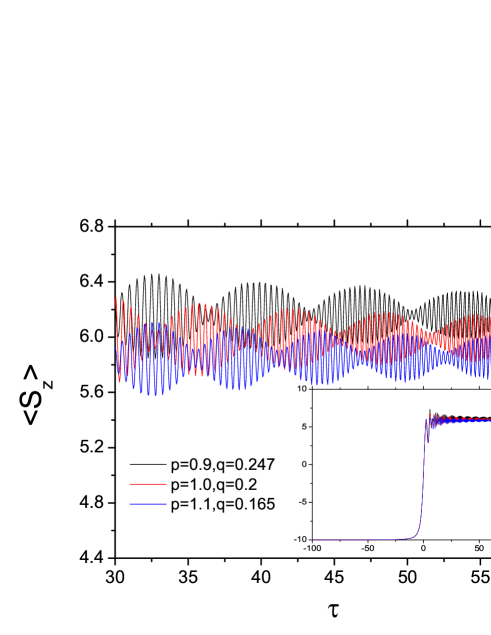
Figure 2: Color online: Time dependence of the average spin of the sample for given values of $p$ and $q$ at $S=10$, $M=0$, and $\gamma=0.02$. Inset: Magnetization step and oscillations in the wider range of $\tau$.

In the absence of transverse terms the energy levels of the Hamiltonian (1) are

$$E_{m}=-Dm^{2}-g\mu_{B}H_{z}m\,,$$ (7)

where $\hat{S}_{z}|m\rangle=m|m\rangle$. Close to the resonance between $|-S\rangle$ and $|S-M\rangle$ the Hamiltonian (5) can be projected onto these states, resulting effectively in a two-level model:

$${\cal{H}}^{(\rm lat)}_{\rm eff}=-{1\over 2}\Delta\hat{\sigma}_{x}-\delta E(\hat{\sigma}_{z}+\hat{I}),$$ (8)

where

$$\delta E=\left(S-{M\over 2}\right)\left[g\mu_{B}ct+{\hbar\omega_{R}\over S}\sin(kx-wt)\right]$$

$$\hat{\sigma}_{z}=|S-M\rangle\langle S-M|-|-S\rangle\langle-S|$$

$$\hat{\sigma}_{x}=|S-M\rangle\langle-S|+|-S\rangle\langle S-M|$$

$$\hat{I}=|S-M\rangle\langle S-M|+|-S\rangle\langle-S|\,,$$ (9)

$\Delta$ is the splitting of the resonant levels, $c=dH_{z}/dt$ is the field sweep rate, and

$$\omega_{R}={\omega^{2}\over 2c_{t}}u_{0}S$$ (10)

is the Rabi frequency. Treating $x$ as a parameter, we express the corresponding wave function as

$$|\Psi^{\rm(lat)}_{\rm eff}(t)\rangle=b_{S-M}(t)|S-M\rangle+b_{-S}(t)|-S\rangle.$$ (11)

and solve the time-dependent Schrödinger equation,

$$i\hbar{\partial|\Psi^{\rm(lat)}_{\rm eff}(t)\rangle\over\partial t}={\cal{H}}^{(\rm lat)}_{\rm eff}|\Psi^{\rm(lat)}_{\rm eff}(t)\rangle\,,$$ (12)

that at $M=0$ becomes equivalent to the following two coupled differential equations:

$${db_{S}\over d\tau} = 2iS\left[\gamma\tau-{qp\over S}\sin(p\tau-{kx})\right]b_{S}+{i\over 2}b_{-S}$$

$${db_{-S}\over d\tau} = {i\over 2}b_{S},$$ (13)

where we introduced dimensionless

$$\tau=t\left(\frac{\Delta}{\hbar}\right),\quad\gamma=\frac{\hbar g\mu_{B}c}{\Delta^{2}},\quad p=\frac{\hbar\omega}{\Delta},\quad q=\frac{\omega_{R}}{\omega}\,.$$ (14)

We consider samples of length that is large compared to the wavelength of the sound. The expectation value of the $z$-projection of the spin at $M=0$ is given by

$$\langle\Psi(t)|\hat{S}_{z}|\Psi(t)\rangle=S\left|b_{S}(\tau)\right|^{2}+(-S)\left|b_{-S}(\tau)\right|^{2}\,.$$ (15)

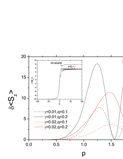
Figure 3: Color online: Final magnetization vs $p$ for the $M=0$ step with and without acoustic wave at different $\gamma$ and $q$. Inset: $\langle S_{z}\rangle$ vs $\tau$ at $\gamma=0.01$, $q=0.2$ and $p=0.9$.

Eqs. (13) have been solved numerically. Fig. 2 illustrates situation when the field was changing at a constant rate $\gamma$ and a pulse of sound was introduced shortly before reaching the resonance between the $|-S\rangle$ and $|S\rangle$ states. The tunnel splitting is assumed to be sufficient to produce transitions between these two states. The most striking feature of the magnetization dynamics observed in simulations are the beats which are in line with the idea outlined in the introduction. Fig. 3 shows the $p$-dependence of the final magnetization on crossing the step for various values of $\gamma$ and $q$. This strong dependence of the magnetization step on frequency and amplitude of the acoustic wave, as well as on the sweep rate, is one of our main results. We believe that it should not be difficult to observe this effect in experiment.

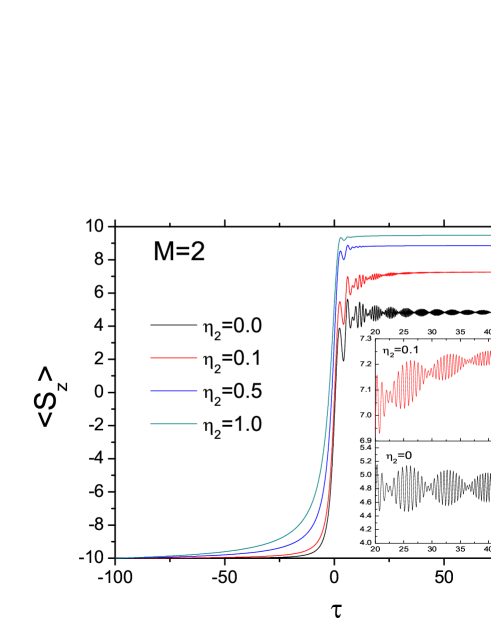
Figure 4: Color online: $\langle S_{z}\rangle$ vs $\tau$ for $\eta_{2}=$ 0, 0.1, 0.5, and 1.0 at $S=10$, $p=0.9$, $q=0.247$, $\gamma=0.02$, and $M=2$. Inset: Oscillations between $\tau=20$ and $\tau=50$ at $\eta_{2}=$0 and 0.1. Note that the beats and the oscillatory behavior disappear as $\eta_{2}$ increases.

Another possible experimental situation corresponds to the sample initially saturated in the $|-S\rangle$ state, after which the acoustic power of frequency $\omega\approx\Delta/\hbar$ is applied to the crystal and maintained during the sweep. Here $|S-M\rangle$ is the level that at a given sweep rate provides significant probability of the transition when it is crossed by the $|-S\rangle$ level. In order to study such a problem, we need to know the rate of relaxation of the $|S-M\rangle$ state to the lower energy states. Defining $\Gamma_{S-M+1,S-M}$ as the rate of the $|S-M\rangle\rightarrow|S-M+1\rangle$ transition and introducing $\eta_{M}=\hbar\Gamma_{S-M+1,S-M}/\Delta$, we obtain two coupled differential equations:

$${db_{S-M}\over d\tau} = izb_{S-M}+{i\over 2}b_{-S},$$

$${db_{-S}\over d\tau} = {i\over 2}b_{S-M},$$ (16)

where

$$z=(2S-M)\left[\gamma\tau-(qp/S)\sin\left(p\tau-kx\right)\right]+i\eta_{M}/2\,.$$ (17)

As the lifetimes of the excited states with $|S-M+1\rangle$,…,$|S-1\rangle$ are shorter than the lifetime of $|S-M\rangle$, their contributions to the above equations can be neglected. Then

$$\langle S_{z}\rangle=-2S|b_{-S}(\tau)|^{2}-M|b_{S-M}(\tau)|^{2}+S$$ (18)

We solve Eqs.(16) numerically for selected values of $\gamma$ and $\eta_{M}$. In the overdamped case, $\Gamma_{S-M+1,S-M}\gg\Delta$, we find no Rabi oscillations. For the underdamped case, $\Gamma_{S-M+1,S-M}\ll\Delta$, the numerical solution is illustrated in Fig. 4. As the damping increases, the magnetization jump becomes more pronounced but the oscillatory dynamics disappears. The comparative behavior of different resonances is shown in Fig. 5.

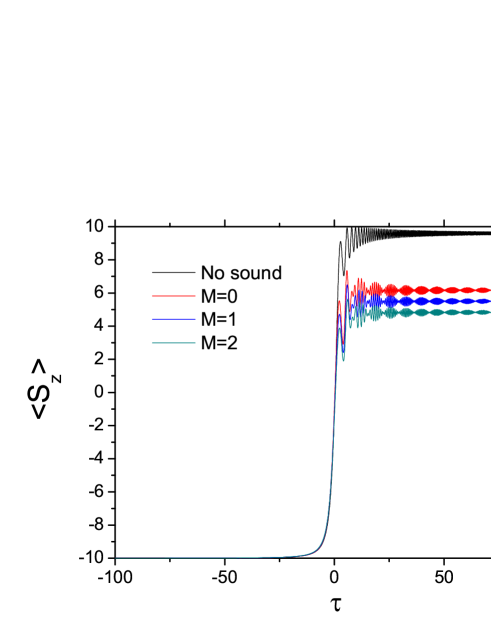
Figure 5: Color online:$\langle S_{z}\rangle$ vs $\tau$ for $M=$ 0, 1, and 2, at $\eta_{M}=0$, $S=10$, $p=0.9$, $q=0.247$, and $\gamma=0.02$.

Let us now study the optimal conditions for the observation of the macroscopic acoustic Rabi effect studied above. Defining $\omega_{q}(\tau,x)\equiv S[\gamma\tau-(qp/S)\sin(p\tau-2\pi x/\lambda)]$ where $\lambda=2\pi/k$ is the wavelength of the sound, the coupled differential equations (13) can be written as

$$\ddot{b}_{S}-2i\omega_{q}\dot{b}_{S}-\left(2i\dot{\omega}_{q}-{1\over 4}\right)b_{S}=0\,,$$ (19)

where $\dot{b}_{S}=db_{S}/d\tau$, $\ddot{b}_{S}=d^{2}b_{S}/d\tau^{2}$ and so on. Introducing $b_{S}=d_{S}\exp[iv(\tau)]$ and selecting $\dot{v}=\omega_{q}$, we get

$$\ddot{d}_{S}+\left(-i\dot{\omega}_{q}+\omega^{2}_{q}+{1\over 4}\right)d_{S}=0\,,$$ (20)

which describes damped oscillations. At $q\neq 0$ we have, e.g., for $x=0$ and $x=\lambda/2$

$$\omega_{q}(\tau,0)=S\left[\gamma\tau-{qp\over S}\sin(p\tau)\right],$$ (21)

$$\omega_{q}(\tau,\lambda/2)=S\left[\gamma\tau+{qp\over S}\sin(p\tau)\right],$$ (22)

respectively. This implies that each frequency generates slow and fast oscillatory regions due to the sinusoidal function, and they show different damped oscillatory structures in a given range of $\tau$. In other words if $\omega_{q}(\tau,0)$ is larger than $\omega_{0}\equiv S\gamma\tau$ in some range of $\tau$, $\omega_{q}(\tau,\lambda/2)$ is smaller than $\omega_{0}$, and vice versa (see Fig. 1). At $\tau\sim 0$ the frequencies are approximately given by $\omega_{q}(\tau,0)\simeq S(\gamma-qp^{2}/S)\tau$ and $\omega_{q}(\tau,\lambda/2)\simeq S(\gamma+qp^{2}/S)\tau$ Introducing $\tan\theta_{1}=\dot{\omega}_{q}(\tau,0)$, $\tan\theta_{2}=\dot{\omega}_{q}(\tau,\lambda/2)$, and $w=qp^{2}/S$, we get

$$|\tan(\theta_{1}-\theta_{2})|=\left|{2w\over 1+\gamma^{2}-w^{2}}\right|,$$ (23)

which increases monotonically in the range of $0<w<1+\gamma^{2}$. Under this condition, let us first consider two limiting cases: $w\gg\gamma$ and $w\ll\gamma$. In the first case $(\theta_{1}-\theta_{2})$ increases with $w$, and thereby $|\omega_{q}(\tau,0)-\omega_{q}(\tau,\lambda/2)|$ also increases, which is a less favorable situation for the beats. In the second case we have $\theta_{1}\simeq\theta_{2}$, which results in $\omega_{q}(\tau,0)\simeq\omega_{q}(\tau,\lambda/2)\simeq\omega_{0}$. This also is not a favorable situation for the beats because it does not generate slow and fast oscillatory regions for $x=0$ and $x=\lambda/2$, as discussed previously. The optimal condition for pronounced beats is then

$$\gamma\simeq{qp^{2}\over S}\,.$$ (24)

Figure 6: Time dependence of the magnetization of the sample for $M=0$ at $S=10$, $\gamma=0.006$, $q=0.01$, and $p=2.45$.

We shall now discuss what the above condition means for experiment. It is easy to see that Eq. (24) is equivalent to

$$\frac{u_{0}}{\lambda}=\frac{q}{\pi S}\,.$$ (25)

The validity of the continuous elastic theory that we employed requires $u_{0}\ll\lambda$, that is, one needs to satisfy the condition $q<1$. This is not sufficient, though. Since experiments on molecular magnets require temperature in the kelvin range or lower, one should also be concerned with the power of the sound. It should be sufficiently low to avoid the unwanted heating of the sample. The power per cross-sectional area of the sample is given by $P/A=\frac{1}{2}\rho u_{0}^{2}\omega^{2}c_{t}$. For, e.g., the parameters of Fe-8 molecular magnet we find that the optimal conditions of the experiment require sound of frequency $f=0.5$MHz -$1$MHz and power in the range $100$W/cm²-$200$W/cm² introduced into the sample simultaneously with the field sweep of $1$kG/s. Time dependence of the magnetization under these conditions is shown in Fig. 6.

In conclusion, we have demonstrated that the size of the magnetization step due to resonant spin tunneling in molecular magnets can be strongly affected by sound. The acoustic wave can also generate macroscopic quantum beats of the magnetization during a field sweep. The required frequency (MHz) and power (0.1kW/cm²) of the sound, and the required sweep rate (1kG/s) are within experimental reach.

The authors are grateful to D. A. Garanin for useful discussions. The work of GHK has been supported by the Grant No. R01-2005-000-10303-0 from Basic Research Program of the Korea Science and Engineering Foundation. The work of EMC has been supported by the NSF Grant No. DMR-0703639.

References

- (1) J. R. Friedman, M. P. Sarachik, J. Tejada, and R. Ziolo, Phys. Rev. Lett. 76, 3830 (1996).
- (2) E. M. Chudnovsky and J. Tejada, Macroscopic Quantum Tunneling of the Magnetic Moment (Cambridge University Press, Cambridge, 1998).
- (3) W. Wernsdorfer and R. Sessoli, Science 284, 5411 (1999).
- (4) E. M. Chudnovsky and D. A. Garanin, Phys. Rev. Lett. 79, 4469 (1997); D. A. Garanin, X. Martínez-Hidalgo, and E. M. Chudnovsky, Phys. Rev. B 57, 13639 (1998); D. A. Garanin and E. M. Chudnovsky, Phys. Rev. B 63, 024418 (2000); G.-H. Kim, Phys. Rev. 59, 11847 (1999).
- (5) A. D. Kent, Y. Zhong, L. Bokacheva, D. Ruiz, D. N. Hendrickson, and M. P. Sarachik, Europhys. Lett. 49, 521 (2000); L. Bokacheva, A. D. Kent, and M. A. Wallis, Phys. Rev. Lett. 85, 4803 (2000); W. Wernsdorfer, M. Murugesu, and G. Christou, Phys. Rev. B 96, 057208 (2006).
- (6) E. M. Chudnovsky and J. Tejada, Lectures on Magnetism (Rinton Press, Princeton, Paramus, NJ, 2006).
- (7) D. A. Garanin and E. M. Chudnovsky, Phys. Rev. B 56, 11102 (1997)
- (8) E. M. Chudnovsky, D. A. Garanin, and R. Schilling, Phys. Rev. B 72, 094426 (2005).
- (9) C. Calero and E. M. Chudnovsky, Phys. Rev. Lett. 99, 047201 (2007).
- (10) A. Hernández-Mínguez, J. M. Hernandez, F. Maciá, A. García-Santiago, J. Tejada, and P. V. Santos, Phys. Rev. Lett. 95, 217205 (2005); F. Maciá, J. Lawrence, S. Hill, J. M. Hernandez, J. Tejada, P. V. Santos, C. Lampropoulos, and G. Christou, Phys. Rev. B 77, 020403 (2008).
- (11) L. D. Landau and E. M. Lifshitz, Theory of Elasticity (Pergamon, New York, 1959).
- (12) E. M. Chudnovsky, Phys. Rev. Lett. 72, 3433 (1994).
- (13) E. M. Chudnovsky, Phys. Rev. Lett. 72, 3433 (1994); E. M. Chudnovsky and X. Martinez-Hidalgo, Phys. Rev. B66, 054412 (2002).