A multi-wavelength survey of AGN in the XMM-LSS field:
I. Quasar selection via the $KX$ technique

Abstract

Aims. We present a sample of candidate quasars selected using the $KX$-technique. The data cover $0.68\deg^{2}$ of the X-ray Multi-Mirror (XMM) Large-Scale Structure (LSS) survey area where overlapping multi-wavelength imaging data permits an investigation of the physical nature of selected sources.

Methods. The $KX$ method identifies quasars on the basis of their optical ($R$ and $z^{\prime}$) to near-infrared ($K_{s}$) photometry and point-like morphology. We combine these data with optical ($u^{*},g^{\prime}r^{\prime},i^{\prime},z^{\prime}$) and mid-infrared ($3.6-24\,\mu m$) wavebands to reconstruct the spectral energy distributions (SEDs) of candidate quasars.

Results. Of 93 sources selected as candidate quasars by the $KX$ method, 25 are classified as quasars by the subsequent SED analysis. Spectroscopic observations are available for 12/25 of these sources and confirm the quasar hypothesis in each case. Even more, 90% of the SED-classified quasars show X-ray emission, a property not shared by any of the false candidates in the KX-selected sample. Applying a photometric redshift analysis to the sources without spectroscopy indicates that the 25 sources classified as quasars occupy the interval $0.7\leq z\leq 2.5$. The remaining 68/93 sources are classified as stars and unresolved galaxies.

1 Introduction

Despite the enormous progress that wide-field imaging surveys have provided in understanding quasar populations over the past decade, concerns remain over the extent to which observational biases contribute to a partial view of the quasar phenomenon. Consequently, multi-wavelength observations are important not only to reproduce the spectral energy distribution (SED) of the objects under study, but also to provide as complete a census as is practical of the quasar population. Nevertheless, selecting source populations using different energy bands encompasses a risk of confusion between different types of objects or different physical processes. Thus, studying the selection effects is an essential step to understanding the properties of the parent population.

A classic method to identify type-1 quasars in optical imaging surveys is known as the $UV$-excess ($UVX$; Sandage 1965, Schmidt & Green 1983). The $UVX$ technique exploits the fact that quasars display an emission excess in blue wavebands compared to main sequence, late type Galactic stars, and therefore occupy a distinct (i.e. bluer) locus in a color-color diagram with respect to stars.

Based on a study of 323 radio-loud sources selected from the Parkes catalog (Wright & Otrupcek, 1990), approximately 70% of which were identified spectroscopically as quasars, Webster et al. (1995) claimed that up to 80% of quasars could be missed in optical surveys. Their suggestion was based on the $B_{J}-K$ color index of these radio-selected sources, which showed a much larger scatter ($1<B_{J}-K<8$) compared to the typical values for optically selected quasars. Various interpretations were suggested, such as (a) intrinsic light absorption, (b) absorption from dust along the line of sight or (c) differences in the internal processes in the active nucleus. Cases (a) and (b) would result in “reddened” quasars, whilst objects in category (c) would be considered as intrinsically “red” (in contrast to the “classical”, blue type-1 quasars).

However, a number of studies have questioned the dusty quasar hypothesis. Masci et al. (1998) rejected the dust hypothesis and Whiting et al. (2001) suggesting that the $B_{J}-K$ spread could be accounted for by synchrotron emission. Benn et al. (1998) claimed that the $B_{J}-K$ scatter could be attributed to observational effects such as variability, underestimated photometric uncertainties, etc. Although Francis et al. (2000) support the conclusions of Webster et al. (1995), Richards et al. (2003) demonstrate that, for the majority of the SDSS quasars, redder colors could be explained by intrinsic processes in the AGN and that the number of missed red and reddened quasars in surveys such as the SDSS (different from typical optical surveys because of the filter selection) comes down to “only” 15%. Brown et al. (2006) found similar results, suggesting that red type-1 quasars correspond to about 20% of the type-1 population.

With the advent of large field, near infrared (NIR) surveys, Warren et al. (2000) suggested a new colour excess criterion, designed to be less prone to the problem of dust reddening and extinction. Their method is the NIR analog of $UVX$: as the quasar SED follows a power-law, it displays a flux excess at NIR wavelengths compared to the Rayleigh-Jeans tail observed in stars. As a result quasars should also occupy a distinct region of the NIR color-color diagram, as they do in the $UBV$ color-color plane. The so-called $K$-excess criterion, hereafter $KX$, would serve as an alternative to the $UVX$ for selecting quasars at redshifts $z>2.2$. At these redshifts, the UV/optical colors of quasars become virtually indistinguishable from those of late type stars.

Despite being a prominsing technique, relatively few $KX$-selected quasar samples have appeared in the literature – mainly due to the considerable effort required to complete a large area NIR imaging survey. The conclusions drawn from the $KX$-selected quasar populations published to date are rather limited as various factors such as the small area of the survey (Croom et al., 2001), the relative shallow magnitudes sampled (Barkhouse & Hall, 2001) or the inhomogeneity and incompleteness of the survey (Sharp et al., 2002) have hampered an assessment of the potential of the method. The first detailed study of the $KX$ method was given by Jurek et al. (2007) while more recently Smail et al. (2008) also published a work on $KX$-selected quasars, raising the problem of contamination by foreground compact galaxies and their impact on spectroscopic follow-up observations.

In this paper we present an analysis of a sample of 93 $KX$-selected quasar candidates selected from 0.68 deg.² of $Rz^{\prime}K_{s}$  imaging data located in the X-ray Multi-Mirror (XMM) Large Scale Structure (LSS) survey field (Pierre et al., 2004). The XMM LSS survey is an X-ray imaging survey covering approximately $10\deg^{2}$ to an approximate point-source flux limit of $8\times 10^{-15}\rm ergs^{-1}cm^{-2}$ in the [0.5-2] keV energy band. The XMM LSS is associated with a number of imaging data sets at different wavebands: the XMM LSS contains the XMM Medium Deep Survey (XMDS), a deeper X-ray imaging component over 2 deg.² in addition to the optical Canada-France-Hawaii Telescope Legacy Survey (CFHTLS) and the Spitzer Wide area IR Extragalactic (SWIRE) survey. These additional data provide a panchromatic view of the quasar candidates and permit a detailed discussion of their physical nature.

The paper is organized as follows: Section 2 presents the optical and NIR data used in the $KX$ technique. Section 3 describes the multi-wavelength data available in the field. Section 4 describes the $KX$ selection criteria and discusses the physical nature of the selected sources using their multi-wavelength properties. In Section 5 we draw some conclusions on the color properties of the confirmed quasars selected using $KX$ and comment on the overall efficiency of the technique. We also consider some of the challenges to be overcome in applying the $KX$ technique to large data sets.

2 Optical and near-infrared observations and data reduction

Two data sets were combined to produce a single optical plus near-infrared catalog upon which to conduct a search for quasars using the $KX$ technique. Optical $R,z^{\prime}$ data were obtained at the Cerro Tololo Interamerican Observatory (CTIO) and near-infrared $K_{s}$-band data were obtained at Las Campanas Observatory (LCO). The two data sets were reduced independently and subsequently matched to form a single catalog. In this section we briefly describe the observations, data reduction and general properties of these photometric data sets.

2.1 Near-infrared observations

Near-infrared observations were performed during the period 25 $-$ 28 October 2002 using the 2.5 m (100 inch) Du Pont telescope, at Las Campanas Observatory. The XMDS field was observed in the $K_{s}$-band, using the Wide Field Infrared Camera (WIRC, Persson et al. 2002). WIRC is a NIR ($1.0-2.5\,\mu$m) camera consisting of four $1024^{2}$ Rockwell HAWAII arrays. Each array covers an area $3.4\times 3.4$ arcmin² with a scale of 0.2^′′/pixel. The four detectors are equally spaced with respect to the center of the configuration, with a gap between them of about 3.05$\arcmin$.

Each telescope pointing consisted of a regular grid of nine dithering pointings with a 20$\arcsec$ offset. A total of $4\times 28\rm s$ exposures were obtained at each dithered location and each combined image displays a total integration time of $9\times 4\times 28\rm s=1008s$ in the central area. The nights of Oct. 25 and Oct. 27 were of mediocre photometric quality, while the nights of Oct. 26 and Oct. 28 were photometric. The typical seeing conditions during the run were between $1.1-1.5^{\prime\prime}$ FWHM. Several hundred images were obtained and then combined to generate a mosaic of 0.8 $\deg^{2}$.

2.2 Optical observations

The full XMDS region was imaged in the $R$- and $z^{\prime}$-bands using the Mosaic II CCD imager mounted on the 4 m Blanco telescope at CTIO observatory. The Mosaic II camera consists of eight $2048\times 4096$ CCD arrays. The scale at the center of the camera is 0.27^′′/pixel, covering in total $36^{\prime}\times 36^{\prime}$ on the sky. The observations were obtained in November 2001 during photometric conditions with an average seeing of FWHM $\approx 1.3\arcsec$. Standard procedures were followed for the reduction of the obtained images.

The CTIO individual frames were astrometrically calibrated using the USNO-2 catalog (Monet et al., 2003) in order to generate mosaic images of the observed area. The final astrometric precision reached was on the order of 0.3^′′. Source extraction and photometry were performed using SExtractor (Bertin & Arnouts, 1996) with independent catalogs generated for each band. Detailed information regarding the data processing of the CTIO data can be found in Andreon et al. (2004).

2.3 Near-infrared data processing

Near-infrared data were processed using a set of scripts based upon the IRAF and PHIIRS (Hall et al., 1998) packages. The reduction strategy is based upon previous near-infrared surveys reported by  Chen et al. (2002) and Labbé et al. (2003). A comprehensive description of the pipeline is given by Nakos (2007) and in this paper we provide a brief description of the data processing sequence.

1. The sky background, residual features and electronic signatures were removed from individual (dithered) frames employing a combination of comparison frames from which objects had been masked.

2. Individual frames were corrected to a uniform photometric sensitivity. Corrections are required to (a) bring all four WIRC detectors to the same sensitivity level, (b) remove differential airmass effects, and (c) calibrate all frames to a standard photometric system. For this purpose, six photometric standard stars (Persson et al., 1998) were observed during the night of October 26. For the two photometric nights these observations were employed to calculate a zero point and extinction coefficient. For the non-photometric nights, the 2MASS photometry (Skrutskie et al., 2006) was used to set the zero point that would shift the instrumental $K_{s}$-band magnitudes to calibrated $K_{s}$-band photometry. Full details about the calibration can be found in Nakos (2007).

3. An astrometric solution was determined for the dithered frames and applied to generate a mosaic image. This was achieved by comparing the coordinates of point-like sources present in the $K_{s}$, 2MASS and $z^{\prime}$-band frames. Having determined the astrometric solution, individual frames were combined to generate four mosaic images.

4. The source completeness and false detection rate in the mosiac images were computed using simulations to determine a suitable magnitude limit in the $K_{s}$-band catalog. As the $K_{s}$  catalog is later matched to the $R$ and $z^{\prime}$ photometric catalogs it is the $K_{s}$-band ’s faintest magnitude that determines the $Rz^{\prime}K_{s}$ survey’s sensitivity limit.

Figure 1: Composite exposure map, generated by combining about 75 individual exposure maps in which the photometric calibration effects (zero point, airmass) have also been incorporated. By dividing the science mosaic by its corresponding composite exposure map we directly derive the calibrated magnitude of the sources in the field. The “sensitivity” of the lighter areas is three times higher to that of the dark areas. Sources lying in the overlapping regions of the mosaic (formed by adjacent pointings) have a better signal-to-noise ratio.

Analysis of the mosaiced images indicated that the impact of the reduction procedure on the photometric uncertainty was at the level of a few hundredths of a magnitude. Exposure mosaics indicating the exact exposure time of pixels in the associated science mosaic were also produced. These frames were used to convert the instrumental magnitudes measured on the science frames into magnitudes in the Vega photometric system. An exposure map of a sub-region of the LCO mosaic image is presented in Fig. 1. The sensitivity ratio between the deepest exposure maps (white) and the shallowest (dark-colored) is on the order of three.

Figure 2: Left panel: Average detection probability, over the four science mosaics, as a function of the $K_{s}$ magnitude (see text for more details). Right panel: Average false detection rate as a function of the $K_{s}$ magnitude. The dashed lines indicate the completeness (left panel) and expected percentage of false detections (right panel) for a catalog cut at $K_{s}=18$.

2.4 Constructing the $K_{s}$-band catalog

Figure 1 indicates that the total exposure time, and therefore the background noise, is not constant over the extent of a given mosaic. Therefore understanding the spatial noise properties of the mosaic is essential for generating the $K_{s}$-band object catalog. The limiting source brightness is determined considering: (a) the probability of detecting a real source, (b) the number of false detections as a function of source brightness. The first condition is required to determine the percentage of sources which are missed as a function of the limiting magnitude of the survey, while the second condition determines the balance between a faint brightness threshold, which will introduce many spurious detections, and a bright threshold which will exclude a significant number of interesting objects.

This study was performed using a code, kindly provided to us by E. Labbe (PUC) and F. Courbin (Ecole Polytechnique Fédérale de Lausanne, Switzerland), that simulates the presence of unresolved sources in our data. Artificial sources are introduced into each science mosaic in a regular grid of locations modulo a small random offset that varies with each simulation. The typical sky area associated with each grid location is 10$\arcsec$. Source extraction is performed on each simulated image and the relative frequency with which the artificial sources are recovered is stored as the detection probability. This process is then repeated for successively fainter artificial sources. The results of the simulations, run on all four mosaics, were averaged in order to obtain a mean value for the detection probability and for the false detection rate. Based on these averaged results, presented in Fig. 2, we concluded that excluding detections fainter than $K_{s}=18$ (within a Kron-type aperture) from the final $K_{s}$-band catalog provides a good balance between a low percentage of false detections (on the order of a few percent) and a satisfactory completeness of the $K_{s}$  catalog (80%). In addition to a magnitude cut, sources with erroneous photometry were removed from the catalog using a combination of SExtractor flag information and visual inspection. Such rejected sources were typically: (a) sources suffering from blending effects due to the presence of a counterpart within a few arcseconds, (b) sources close to saturated objects, (c) sources close to the mosaic borders, or (d) sources affected by bad columns or other artifacts.

The final $K_{s}$-band catalog contains the position (RA,Dec) and the fixed aperture (3^′′ diameter) photometry of some $\sim$4500 entries. These entries were selected according to: (a) their Kron magnitude (the one used during the simulations), and (b) the detection probability corresponding to the position of each detection in the mosaic images (as derived from the simulations).

2.5 Matching the $Rz^{\prime}K_{s}$ catalogs

Source extraction and photometry was performed using SExtractor for the optical $R$ and $z^{\prime}$ image mosaics using similar parameters and checks as used for the $K_{s}$ data. Source photometry in each band was combined into a single catalog by matching the source astrometry in each band within a specified $2\arcsec$ tolerance. The tolerance value was specified considering the astrometric precision of the catalogs and the object density in the LCO field: $R,z^{\prime}$ counterparts were identified for all $K_{s}$-band detections, even those with a poorer astrometric accuracy than average (0.5″), with a minimum risk of misidentification among the few cases of blended objects that were not removed throughout the “cleaning” process described above. The final matched catalog contains some 3400 sources and general catalog properties are presented in Table 1.

Matched sources were classified as point-like or extended on the basis of the $R$- and $z^{\prime}$-band magnitude and the SExtractor stellarity index. It should be noted that although the stellarity index provides reliable information concerning the morphology of relatively bright sources (typical magnitudes $R,z^{\prime}<22$), it is less relaible when considering fainter sources. A combination of the stellarity index and source magnitude provides a more reliable morphological classification. Additional details can be found in Andreon et al. (2004). Out of the 3400 sources in the matched $Rz^{\prime}K_{s}$ catalog some 2450 ($\sim 72$%) were classified as extended, while the remainder were classified as point-like.

Table 1: General properties of the $K_{s}$-band selected $Rz^{\prime}K_{s}$ survey. The astrometric and photometric precision are quoted at $1\,\sigma$.

Filter	Astr. prec.	Phot. prec.	Mag limit
$R$	0.3′′	0.02	22.5
$z^{\prime}$	0.3′′	0.02	21.0
$K_{s}$	0.5′′	0.07	18.0

The final matched catlogue features 3^′′ aperture photometry for all bands where the photometry is computed using the magnitude of Vega as a zero-point. Fig. 3 shows the ($R-z^{\prime}$) vs ($z^{\prime}-K_{s}$) color-color diagram, where the majority of point-like and extended sources occupy distinct regions. Despite the clear separation of the two populations a small fraction of point sources overlap with the extended ones and vice-versa, possibly reflecting uncertainties in the photometry or the morphological classification as well as intrinsically distinct populations.

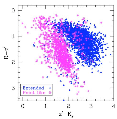
Figure 3: ($R-z^{\prime}$) vs ($z^{\prime}-K_{s}$) diagram for the LCO point-like (asterisks) and extended sources (triangles). The computed colors are based on the 3^′′ photometry (Vega magnitudes). The point-like sources (mainly stars) form a locus well separated from the region occupied by the extended sources (galaxies). For comparison we kept the axis convention of Fig. 2 from Warren et al. (2000), i.e. the vertical axis increases from top to bottom.

3 Multi-wavelength data within the XMDS field

This paper is primarily concerned with the properties of a quasar sample selected using a variant of the $KX$ method, i.e. employing the $Rz^{\prime}K_{s}$ colors of optically point-like sources in the XMDS field. In order to discuss the physical nature of the $KX$-selected quasar sample we will use photometric information at other wavelengths in order to construct low resolution spectral energy distributions (SEDs) for the candidate quasars. In addition, in order to discuss any possible bias in a $KX$-selected quasar sample, we will also compare the $KX$-selected sample to quasar samples selected in the mid-infrared waveband.

We begin by providing a description of the X-ray data products provided by the XMDS itself. In addition, the CFHT Legacy Survey (CFHTLS) and the Spitzer Wide-area InfraRed Extragalacic survey (SWIRE) are two “legacy”-type surveys that overlap the XMM Medium Deep Survey (XMDS) field. We provide below a brief description of the data products associated with these surveys. Detailed information can be found in Tajer et al. (2007) and references therein.

The XMDS was conducted between July 2001 and January 2003 using the European Photon Imaging Camera (EPIC) on board the XMM–Newton satellite (Turner et al., 2001; Strüder et al., 2001). It consists of 19 overlapping pointings (of typical exposure time $20-25$ ksec) covering a contiguous area of $\sim 2$ deg². The energy range of the EPIC instruments is between 0.1 to 12 keV. A detailed description of the pipeline used for reducing the X-ray observations and the catalog properties can be found in Chiappetti et al. (2005). The X-ray source sample used in the present paper was generated from the Chiappetti et al. (2005) source list by selecting unresolved sources displaying more than 20 counts in the B ($0.5-2$) keV energy band. This generated 370 X-ray sources in the $Rz^{\prime}K_{s}$ catalog area.

The XMM-LSS survey (of which the XMDS is a subset) is coincident with the Wide Synoptic component of the Canada France Hawaii Telescope Legacy Survey1 (CFHTLS-W1) (Gwyn, 2007). CFHTLS-W1 $u^{*},g^{\prime},r^{\prime},i^{\prime},z^{\prime}$ photometry is available for approximately 90% of the area covered by the $Rz^{\prime}K_{s}$ observations. The magnitude limit of the survey, at 50% completeness, for a point source observed in seeing of FWHM=0.8^′′ and a signal-to-noise ratio of 5 ($1.5\arcsec$ aperture photometry), is 26.4, 26.6, 25.9, 25.5 and 24.8 for the $u^{*},g^{\prime},r^{\prime},i^{\prime}$ and $z^{\prime}$ bands respectively (AB magnitudes).

SWIRE (Lonsdale et al. 2003, 2004) is the largest Legacy Program performed with the Spitzer Space Observatory (Surace, 2004). Once again, 90% of the sky area associated with the $Rz^{\prime}K_{s}$ catalog is covered by SWIRE data. The $5\sigma$ sensitivity for the 3.6, 4.5, 5.8, 8.0 and 24 $\mu m$  energy bands are 7.3, 9.7, 27.5, 32.5 and 450 $\mu$Jy, respectively (Lonsdale et al., 2003). Throughout this work we shall use the IRAC photometry measured within a 3^′′ aperture; for the MIPS 24 $\mu m$  band the fluxes presented are those measured using a 7.5^′′ diameter.

4 A $KX$-selected quasar sample

The original $KX$ method by Warren et al. (2000) made use of the $V$, $J$ and $K$ bands, noting that quasars with a $V-J$ color similar to that of stars would be redder in $J-K$, a method equally well suited for the detection of reddened quasars according to the authors. In the present work we implement a variant of the original $KX$ technique, using the ($R-z^{\prime}$) versus ($z^{\prime}-K_{s}$) diagram instead.

4.1 Seperating quasars from the stellar locus

Unresolved sources in the $Rz^{\prime}K_{s}$ plane essentially consist of stars, quasars and unresolved galaxies. The properties of the stellar locus on the $Rz^{\prime}K_{s}$ plane were computed using the Pickles (1998) library of 130 stellar spectra (Fig. 4). The locus of stellar photometry was then extended along the $z^{\prime}-K_{s}$  axis to display a half-width of $3\sigma$, where $\sigma$ is the photometric error on the ($z^{\prime}-K_{s}$) color index that dominates the photometric uncertainty in the stellar locus (see also Table 1). Consideration of the relative properties of the SEDs of stars and quasars indicates that quasars should be located toward $z^{\prime}-K_{s}$  colors redder than the stellar locus in Fig. 4. We therefore identify candidate quasars as unresolved sources displaying

$$(R-z^{\prime})=0.6\,(z^{\prime}-K_{s})-0.243\hskip 17.07182pt\mathrm{for}\hskip 5.69046pt(z^{\prime}-K_{s})<2.0,$$ (1)

$$(R-z^{\prime})=2.877\,(z^{\prime}-K_{s})-4.797\hskip 5.69046pt\mathrm{for}\hskip 5.69046pt2.0\leq(z^{\prime}-K_{s})\leq 2.4,$$ (2)

$$(R-z^{\prime})=0.109\,(z^{\prime}-K_{s})+1.983\hskip 17.07182pt\mathrm{for}\hskip 5.69046pt(z^{\prime}-K_{s})>2.4.$$ (3)

These selection criteria identify 93 candidate quasars.

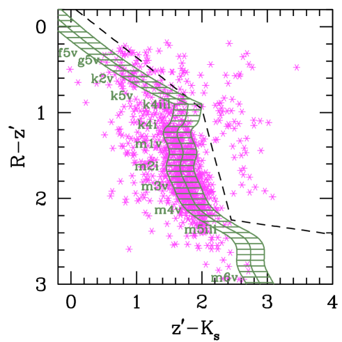
Figure 4: Simulated stellar colors (shaded region) and distribution of the unresolved sources on the $Rz^{\prime}K_{s}$  plane. The dashed line indicates the adopted color threshold seperating stellar and non-stellar sources given by Equations 1-3.

.

4.2 SED analysis of quasar candidates

In the absence of low- to medium-resolution spectroscopy we investigate the nature of the candidate quasar sample via analysis of their UV to MIR SEDs. The $Rz^{\prime}K_{s}$ catalog was therefore matched to the CFHTLS and SWIRE catalogs in order to reconstruct the SED of the objects. The CFHTLS catalog was matched to the $Rz^{\prime}K_{s}$ detections using a matching radius of 2^′′. Thanks to the large overlap between the two sets of observations, CFHTLS $u^{*},g^{\prime},r^{\prime},i^{\prime},z^{\prime}$ counterparts were found for 86/93 quasar candidates. Furthermore, 90/93 quasar candidates are matched to SWIRE sources using a tolerance of $1.5\arcsec$ and show emission in the first two IRAC bands (IRAC 1 = 3.6 $\mu m$ , IRAC 2 = 4.5  $\mu m$ (Fazio et al., 2004)). At longer wavelengths, however, the number decreases significantly with $\sim 30$% of the candidates showing emission in the IRAC 3 (5.8 $\mu m$) and IRAC 4 (8.0 $\mu m$) band and only 16% with emission in the MIPS 24 $\mu m$  channel (Rieke et al., 2004). Therefore, the SED of the quasar candidates will include up to 13 photometric points ($u^{*},g^{\prime},r^{\prime},R,i^{\prime},z^{\prime},z^{\prime}_{ctio},K_{s}$, IRAC 1, 2, 3  4 and MIPS 24 bands), spanning the range $0.4-24\,\mu m$.

The investigation of the candidate quasars sample was performed initially via a visual inspection of their SEDs. Quasar SEDs exhibit two unmistakable signatures in the UV/optical/IR domain: i) the UV/optical-bump customarily attributed to the accretion process; and ii) the minimum (in $\lambda F_{\lambda}$) or break with subsequent change of slope (in $F_{\lambda}$ or $F_{\nu}$), occurring at around 1 micron (see Hatziminaoglou et al. 2005; Richards et al. 2006), where the drop of the accretion bump meets with the T $\sim 1500$ K black-body rise (towards the IR), corresponding to the graphite grains believed to be one of the two main components of the dusty tori surrounding the active nucleus. This visual inspection yielded 25 quasars among the 93 candidates. The remaining sources were characterised as late type stars and (low redshift) galaxies, characterised either as early-type or starburst-type. The SED of elliptical galaxies peaks around 2 to 3 micron and then decreases monotonically towards redder wavelengths, while that of starbursts shows an excess in the IRAC 4 band due to the strong PAH emission centered at 7.7 micron (Weedman et al., 2006). For the quasars, 22/25 ($\sim 82$%) are “classical” (i.e. blue) type-1, and one ($\sim 6$%) is of type-2 (as its flux experiences a significant attenuation at bluer wavelengths). Although, at present, there is no clear definition of a red quasar (Canalizo et al. 2006 and references therein), there is no doubt that there exists a fraction of quasars where the optical spectrum deviates significantly from that of a type-1 object (e.g. Pierre et al. 2001; Leipski et al. 2007). Two entries in our quasar sample belong to this category, showing a signature of moderate reddening with a flat SED blue-ward of the $\sim$1 $\mu m$ inflection. The lack of spectroscopic information and the small number of objects do not allow any firm conclusion regarding the origin of the flattening of their optical SED. A possible explanation could be the presence of a moderate amount of dust along the line of sight to the active nucleus. In this scenario the dust would affect differentially the blue and red light emitted by the quasar, making the SED appear flatter compared to that of a blue type-1 quasar, but not as steep as that of a type-2. However, larger numbers of sources displaying this feature would be needed before claiming any robust conclusion. The results of the SED inspection are presented in Table 2 and examples of visually classified SEDs are shown in Fig. 5.

Table 2: Results of the SED inspection for the 93 quasar candidates.

SED type	Number
QSO Type-1	22
QSO Type-1 (reddened)	2
QSO Type-2	1
Galaxy	50
Star	18

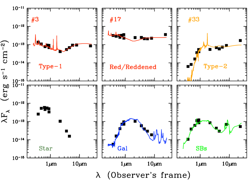
Figure 5: Upper Panel: Typical examples of the Spectral Energy Distribution of: a “blue” type-1 quasar (left), a quasar showing significant reddening signature (middle) and of the single type-2 quasar found in the LCO survey (right). In each case the best-fit template (as derived from the HyperZ calculation – see Section 4.6) is also plotted. Objects #3, #17 and #33 are found at redshifts of 1.513, 0.710 and 1.679, respectively. Lower Panel: SED of a star (left), an elliptical galaxy at redshift $z=0.545$ (middle) and a galaxy showing starburst activity at $z=$0.127.

4.3 The MIR color-color diagram

The $KX$ method seperates quasars and stars on the basis of their optical and near-infrared colors. An alternative method applies the same test on the mid-infrared colour plane. Hatziminaoglou et al. (2005) demonstrated that it is possible to isolate type-1 quasars using the first three IRAC bands (3.6, 4.5 and $5.8\,\mu m)$. These bands seperate quasars from stars as they sample the stellar Rayleigh-Jeans tail of the blackbody spectrum. As a result, the stellar colors are very close to zero in the Vega photometric system. Following their approach, we constructed the MIR color-color diagram for all unresolved sources in the $Rz^{\prime}K_{s}$ catalog (Fig. 6). Three sources classified as stars on the basis of their $Rz^{\prime}K_{s}$ photometry are located in the so-called “quasar locus” and visual inspection of their SEDs confirms the quasar hypothesis. Of these sources, two are located very close (about 0.2 mag in each direction) to the stellar locus on the $Rz^{\prime}K_{s}$ plane. The third source is an isolated quasar located in the stellar locus of Fig. 3, for which we possess a spectroscopic identification (see section 4.4). We finally note that two sources classified as quasars on the basis of their $Rz^{\prime}K_{s}$ photometry and SED analysis lie outwith yet close to the quasar locus defined by Hatziminaoglou et al. (2005).

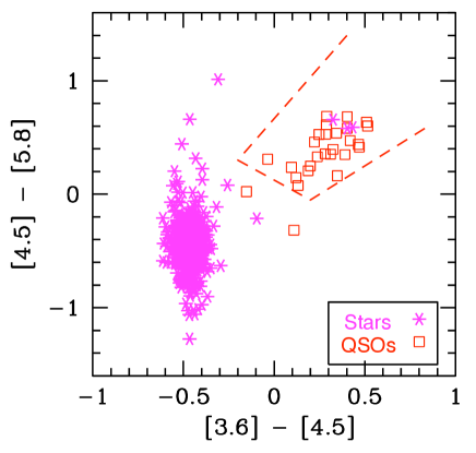
Figure 6: SWIRE color-color diagram for unresolved sources in the $Rz^{\prime}K_{s}$ catalog. Sources classified as stars are displayed as asterisks and sources classified as quasars (on the basis of $Rz^{\prime}K_{s}$ colors and SED inspection) are plotted as open squares. According to Hatziminaoglou et al. (2005) quasars are expected to be found in the region delineated with the long-dashed line. Visual inspection of the SED of the three “stars” within the quasar locus confirms the quasar hypothesis.

4.4 Spectroscopy of quasar candidates

To date it has not been possible to perform a systematic spectroscopic investigation of the $KX$-selected quasar sample presented in this paper. However, a number of spectroscopic programs have been performed which overlap the XMDS area with the result that spectroscopic information is available for a subset of sources presented in this paper. As part of the spectroscopic identification program for the XMM-Newton Survey Science Centre medium sensitivity serendipitous survey Tedds et al. (2006), the two degree field multi object spectrograph (2dF, Lewis et al. 2002) targeted some 800 X-ray detected sources with $r_{AB}<22$ including the XMM-LSS area. More details about the 2dF program will be given in a forthcoming X-ray Wide Area Survey (XWAS) catalog paper (Tedds et al. in prep.). A total of 22 sources with 2dF spectra were associated with sources in the $Rz^{\prime}K_{s}$ catalog. These included one star, 9 quasars and 12 galaxies as classified by their $Rz^{\prime}K_{s}$ photometry. In each case the spectroscopic classification matched the $Rz^{\prime}K_{s}$ classification. A further five spectra were available for sources with $K_{s}>18$ and therefore not included in the $Rz^{\prime}K_{s}$ catalog. These sources were classified as type-1 quasars. They are not used further in the analysis, except as part of a spectral training set for the photometric redshift analysis (Section 4.6). Three examples of good-quality 2dF spectra are presented in Fig. 7.

Figure 7: Examples of good-quality 2dF spectra used to investigate $Rz^{\prime}K_{s}$ sources. The identification of each object is presented in the upper left part of each spectrum; some of the spectral features employed to classify each source are also shown. Object # 528 is a star, object # 735 a quasar at $z=0.76$ and object # 243 a galaxy at $z=0.263$ (Garcet et al., 2007).

A further four sources classified as quasars on the basis of their $Rz^{\prime}K_{s}$ photometry and SED analysis have been confirmed spectroscopically as type-1 quasars (source numbers 2, 3, 20 and 27 in Table 2). Observations were conducted as part of the VLT/VIMOS program (080.A-0852B) to investigate X-ray selected AGN in the XMM-LSS survey area (Garcet et al. in prep.).

Therefore, for the $KX$-selected quasar sample, 12/25 sources classified as quasars on the basis of $Rz^{\prime}K_{s}$ photometry and SED analysis have been confirmed spectroscopically. However, it is important to note that the spectroscopic programs that observed these sources were constructed to investigate X-ray selected source samples. It is therefore important at this stage to consider the X-ray properties of the $KX$-selected quasar sample.

4.5 X-ray properties of the quasar sample

As noted in Section 3, there are 370 X-ray sources in the overlapping XMDS and $Rz^{\prime}K_{s}$ catalog area. Of these, 81 X-ray sources were matched to a single $Rz^{\prime}K_{s}$ source within a $7\arcsec$ matching radius. This radius was chosen on the basis of: (a) the density of X-ray detections; (b) the accuracy of the X-ray astrometric solution ($\sim 1^{\prime\prime}$); and (c) XMM-Newton’s point spread function ($6\arcsec$).

The relatively low fraction of matched sources, 81/370, is largely due to the shallow depth of the $K_{s}$ band observations compared to the optical observations. Approximately 20% of the $KX$-selected quasar sample, 21/93, are matched to an X-ray detection. Of these matched sources, 12/13 are spectroscopically confirmed quasars and 21/25 are SED classified quasars (note that the SED classified quasars include all of the spectroscopically confirmed quasars as well). None of the sources classified as stars or galaxies as a result of the SED inspection have an X-ray counterpart.

We intend to discuss the X-ray properties of the $KX$-selected quasar sample in greater detail in a subsequent paper. However, at this point we note that the X-ray-to-optical flux ratios of the SED-classified quasars occupy the interval $0.1<\log(F_{X}/F_{R})<10.0$, typically occupied by AGN (Della Ceca et al., 2004). Figure 8 indicates that the four sources classified as quasars yet lacking an X-ray counterpart are consistent with being drawn from the same population as the X-ray detected quasars if we consider that application of the above X-ray-to-optical flux ratio would place the X-ray fluxes for these four sources below the nominal flux limit of the XMDS X-ray source catalog.

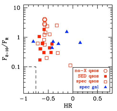
Figure 8: Plot of the X-ray to optical flux ratio for SED and spectroscopically classified quasars and spectroscopically classified galaxies (from the 2dF sample) versus X-ray hardness ratio. Hardness ratio is computed according to Equation 2 of  Garcet et al. (2007). The four quasar candidates that are undetected in X-rays are plotted as upper limits on $\rm F_{2-10}/F_{R}$ with the median HR value of the X-ray detected quasar sample. The region enclosed by the dashed rectangle indicates the anticipated locus of X-ray emitting stars.

Therefore, for the sample of 93 $KX$-selected quasars, 21/25 of the sources classified as quasars from the SED analysis show X-ray emission. The remaining four sources are consistent with being drawn from the same population. None of the 68 remaining sources classified as either stars or galaxies from the SED analysis is detected in X-rays. We therefore conclude that the X-ray properties of the $KX$-selected quasar sample support the previous conclusions on the nature of individual sources derived from the SED analysis.

4.6 Photometric redshift analysis

In the absence of complete spectroscopic informtion for the 93 sources in the $KX$-selected quasar sample we employed the HyperZ code (Bolzonella et al., 2000) to compute photometric redshifts. The spectral templates applied to the data are described in Polletta et al. (2007) and cover the wavelength interval 100 nm $-$ 100 $\mu$m. We tested the performance of HyperZ by first running the program on the 14 quasars with 2dF spectra, using various combinations of filters, reddening laws and templates. Based on the limiting magnitude of the $Rz^{\prime}K_{s}$ survey and the maximum spectroscopic redshift in our catalog, we set $z_{max}=3.0$. As HyperZ is limited to 15 templates per run, we selected five quasar templates (three type-1 and two type-2) while the remainder were selected among the templates for elliptical, starburst, Seyfert and spiral galaxies.

The performance of the photometric redshift method was estimated on the basis of two parameters: the fractional error $\Delta z$ and the $1\sigma$ dispersion $\sigma_{z}$ as defined by Tajer et al. (2007),

$$\Delta z=\left(\frac{z_{phot}-z_{spec}}{1+z_{spec}}\right)\hskip 14.22636pt\mathrm{and}\hskip 14.22636pt\sigma_{z}^{2}=\frac{1}{N}\sum\left(\frac{z_{phot}-z_{spec}}{1+z_{spec}}\right)^{2}$$ (4)

where $N$ is the number of sources with spectroscopic redshifts. After various trials we obtained a photometric redshift for 12 of the 14 sources with $\left|\Delta z\right|<0.3$ and $\sigma_{z}=0.19$.

The remaining 16 quasars without spectra consists of 15 type-1 and one type-2 object (#33), characterized as such on the basis of their SED. The best-fit template matched by HyperZ was in very good agreement with the SED-based classification, fitting the ID #33 quasar with a type-2 spectral template and 13 out of 15 type-1 objects with a type-1 spectral template. Only two type-1 objects were fit by a Seyfert 1.8 template (#27 and #57). Figure 9 shows the template fitting results for the full sample of 93 quasar candidates. Although the upper limit for the $A_{V}$ extinction coefficient was set to 0.5 no object was found to have $A_{V}>0.4$, with 13 out of 19 objects having $A_{V}<0.2$. Finally, the $B$-band absolute magnitude was set to vary between $-23.0<M_{B}<-28.8$, but no object was found to have an absolute magnitude brighter than $M_{B}=-26.22$. The final photometric redshifts for the 16 newly discovered quasars are presented in Table 5.

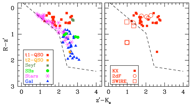
Figure 9: Left panel: Distribution in the color-color diagram of the initial sample of 93 quasar candidates. The color-coding is based on the best-fitting SED returned via the photometric redshift analysis. The dashed line indicates the border between the stellar and non-stellar colors used in our selection procedure. Right panel: Color-color diagram containing the quasars detected using jointly several methods (2dF, $KX$, SWIRE). The $KX$-selected quasars are marked with filled squares while the open circles denote the 6 quasars with 2dF spectra not selected by the $KX$. Three type-1 quasars, selected on the basis of their IRAC colors, are marked as open squares. The isolated object at $(R-z^{\prime})\approx 1.7$ is the type-2 $KX$-selected quasar found in our survey.

5 Conclusions

The distribution in $Rz^{\prime}K_{s}$ for the 93 quasar candidates is shown in the left panel of Fig. 9. The distribution of all quasars found in the $Rz^{\prime}K_{s}$ catalog, using $KX$-selection plus SED analysis, 2dF spectra (subsection 4.4) and IRAC colors (subsection 4.3) is presented in the right panel of the same figure. The first conclusion to be drawn from these two plots is that the majority of the quasar population (type-1) is concentrated in the bluer part of the ($R-z^{\prime}$) axis, with the ($R-z^{\prime}$) color ranging from 0.2 to 0.8 magnitudes. This occurs as the quasar power-law SED produces an excess in the $K_{s}$-band, with the result that quasars appear redder than stars along the $z^{\prime}-K_{s}$ axis. In addition, the same power-law SED causes quasars to appear bluer than galaxies. We note the presence of a single type-2 quasar detected by the $KX$-method. This object is much redder, with $R-z^{\prime}$$\approx 1.7$, and would have been missed if stricter color criteria had been applied, e.g. a bluer cut in $R-z^{\prime}$.

To assess the performance of the $KX$-method in a quantitative manner we adopt the formalism presented in Hatziminaoglou et al. (2000). Defining $N_{c}$ as the number of quasar selected candidates, $N_{f}$ as the number of quasars confirmed from the candidates and $N_{e}$ as the number of expected quasars (based upon model predictions), one may define the efficiency, $E$, of the technique as

$${E=\frac{N_{f}^{2}}{N_{e}N_{c}}.}$$ (5)

The $KX$-method identified 25 quasars in an area of 0.68 deg² at $K_{s}<18$. The $Rz^{\prime}K_{s}$ catalog is 80% complete at $K_{s}=18$ and therefore the effective surface density of $KX$-selected quasars at $K_{s}<18$ is $46\pm 9\deg^{-2}$. Maddox & Hewett (2006) use model predictions to estimate a quasar surface density at $K_{s}<18$ of $50\deg^{-2}$. Employing these values, the completeness of the $KX$-selected sample is on the order of 90%. The identification of 25 quasars from the 93 candidates indicates a confirmation rate on the order of 27%. Therefore, employing Equation 5, the overall efficiency of the $KX$-techniqe as applied in this paper is approximately 25%.

Detailed studies of quasar populations represent a key component of the current generation of wide-field optical to MIR imaging surveys. Selection by color provides an important technique for compiling large samples of quasar candidates. However, the application of color criteria alone are unlikely to generate uncontaminated quasar samples. SED classification of quasar candidates may provide an important technique for prioritizing the spectroscopic observations of large quasar samples – with the potential to improve considerably the efficiency of follow-up programs. Throughout the present analysis we have applied a visual classification of candidate quasar SEDs. Clearly an automated approach will be required for larger samples. Large surface IR surveys, such as UKIDSS (Hewett et al., 2006), will base their quasar selection on the $KX$ technique. Because of the depth of the surveys and the large area coverage (several thousand square degrees) it would be advantageous to minimize contamination prior to spectroscopic confirmation.

Appendix A Details concerning the photo-z calculations

In this appendix we present in detail the parameters used for computing the photometric redshifts of the quasars found in our survey, for which no spectroscopic information was available.

HyperZ was fed with 15 templates, taken from the Polletta et al. (2007) library. They were chosen from seven different categories of active (AGN) or non-active (ellipticals, spirals) galaxies. Concerning the starburst galaxies, the templates are those of Arp 220, M 82 and NGC 6090. The exact number of templates per category is presented in Table 3.

The minimum and maximum redshifts were 0.7 and 3.0, respectively, with a step of $\Delta z=0.01$.

In the photo-z computation, the possibility of dust reddening was incorporated via the Calzetti et al. (2000) reddening law. The minimum and maximum reddening values were 0.0 and 0.5, respectively, with a step of 0.1.

Constraints were also set on the absolute $M_{B}$-band magnitude of the sources. We used the $g^{\prime}$-band filter as a reference and computed the approximate limits in this band considering the formula by Smith et al. (2002):

$$B=g^{\prime}+0.47\,(g^{\prime}-r^{\prime})+0.17$$ (6)

with $-28.0\leq M_{B}\leq-22.0$ and using an average $(g^{\prime}-r^{\prime})_{AB}$ color index of 0.65. Based on the output of HyperZ, the brightest absolute magnitude was found to be $M_{B}=-25.42$ and the faintest $M_{B}=-22.5$, respectively.

The cosmological parameters used in this analysis are $H_{0}=70$ km s^-1 Mpc^-1, $\Omega_{\Lambda}=0.7,\,\Omega_{M}=0.3$.

Table 3: Distribution of the template categories used for the photometric redshift calculations.

Template type	Nr
Type-1 quasar	3
Type-2 quasar	2
Seyfert	2
Starbursts	3
Ellipt.	3
Spirals	2

Table 4: Sources in the LCO field with a 2dF spectroscopic identification. Column 1 gives the identifier of the source in the spectroscopic data base. Columns 2 and 3 give the right ascension and declination of each source, for equinox 2000. Columns 4, 5 provide the spectroscopic classification of the source (Star, Quasar or Galaxy) and its measured redshift (for the latter two object-types), respectively. The typical uncertainty on the estimated redshift is on the order of 0.001 and 0.005 for the galaxies and quasars, respectively. Columns $6-7$, $8-9$ and $10-11$ give the 3^′′ photometry and its error for the $R,z^{\prime}$ and $K_{s}$-bands, respectively. Columns $11-12$ provide the ($R-z^{\prime}$) and ($z^{\prime}-K_{s}$) color index for each source, respectively. The five quasars not included in the matched $Rz^{\prime}K_{s}$ catalog are presented at the bottom of Table 4 and are marked as “Q*”.

ID	RA (J2000)	Dec (J2000)	Type	Rdsft	$R$	$\sigma_{R}$	$z^{\prime}$	$\sigma_{z^{\prime}}$	$K_{s}$	$\sigma_{K_{s}}$	$R-z^{\prime}$	$z^{\prime}-K_{s}$
	h m     s	${}^{\circ}\hskip 8.53581pt{}^{\prime}\hskip 8.53581pt{}^{\prime\prime}$
528	2 22 55.08	$-$4 12 10.58	S	$-$	19.012	0.002	17.359	0.001	14.949	0.021	1.654	2.410
735	2 22 44.40	$-$4 33 47.02	Q	0.760	18.307	0.001	18.510	0.003	16.309	0.034	$-$0.203	2.201
736	2 22 47.90	$-$4 33 30.20	Q	1.629	20.151	0.006	20.122	0.013	17.900	0.128	0.029	2.222
97	2 23 26.47	$-$4 57 06.30	Q	0.826	20.994	0.013	20.968	0.029	17.843	0.135	0.026	3.125
100	2 23 54.82	$-$4 48 15.19	Q	2.463	18.163	0.001	18.371	0.003	16.092	0.023	$-$0.208	2.279
251	2 24 29.14	$-$4 58 08.11	Q	1.497	19.626	0.004	19.959	0.011	17.907	0.101	$-$0.333	2.052
23	2 25 14.40	$-$4 47 00.38	Q	1.924	19.225	0.003	18.456	0.004	16.918	0.045	0.769	1.538
41	2 25 40.61	$-$4 38 25.30	Q	2.483	19.860	0.005	19.898	0.013	17.625	0.096	$-$0.038	2.273
11	2 25 56.83	$-$4 58 53.29	Q	1.183	20.947	0.014	21.147	0.039	17.968	0.127	$-$0.200	3.179
14	2 25 57.62	$-$4 50 05.50	Q	2.263	19.454	0.004	19.722	0.011	17.826	0.084	$-$0.268	1.896
531	2 22 57.98	$-$4 18 40.50	G	0.237	19.047	0.003	18.112	0.002	14.674	0.010	0.935	3.438
544	2 23 02.04	$-$4 32 04.81	G	0.616	20.437	0.008	20.004	0.012	16.767	0.040	0.433	3.237
742	2 23 15.36	$-$4 25 58.69	G	0.190	19.695	0.004	19.423	0.007	17.099	0.064	0.272	2.324
743	2 23 19.66	$-$4 47 30.80	G	0.293	19.284	0.003	18.798	0.004	15.651	0.045	0.486	3.147
96	2 23 44.26	$-$4 57 25.42	G	0.157	19.803	0.005	19.576	0.008	16.635	0.034	0.227	2.941
65	2 23 51.29	$-$4 20 53.41	G	0.181	19.635	0.004	19.666	0.009	17.144	0.056	$-$0.031	2.522
125	2 24 18.79	$-$5 01 20.89	G	0.458	20.769	0.011	20.589	0.020	18.177	0.141	0.180	2.412
248	2 25 21.07	$-$4 39 49.90	G	0.265	19.416	0.003	18.941	0.005	16.074	0.048	0.475	2.867
243	2 25 24.70	$-$4 40 44.69	G	0.263	19.044	0.003	18.448	0.004	15.412	0.017	0.596	3.036
46	2 25 31.39	$-$4 42 20.30	G	0.209	20.015	0.006	19.929	0.013	17.806	0.074	0.086	2.123
42	2 25 32.02	$-$4 43 46.20	G	0.314	20.224	0.007	19.731	0.011	16.929	0.048	0.493	2.802
357	2 25 58.87	$-$5 00 54.50	G	0.148	18.324	0.001	17.921	0.002	15.106	0.029	0.403	2.815
530	2 22 49.63	$-$4 13 52.97	Q*	1.566	20.301	0.007	20.461	0.018	17.793	0.087	$-$0.160	2.668
281	2 23 51.10	$-$4 47 29.76	Q*	2.164	20.065	0.005	20.311	0.015	18.001	0.101	$-$0.246	2.310
91	2 23 58.66	$-$4 53 51.40	Q*	2.275	19.866	0.004	20.084	0.012	17.509	0.066	$-$0.218	2.575
271	2 24 13.46	$-$4 52 10.27	Q*	2.487	20.646	0.009	20.913	0.026	18.097	0.110	$-$0.267	2.816
375	2 25 37.03	$-$5 01 09.41	Q*	1.937	19.968	0.005	19.953	0.013	18.076	0.106	0.015	1.877

Table 5: Astrometry and optical photometry for the 19 type-1 and type-2 newly discovered quasars in a sub-region of the XMM-LSS field. Column 1 gives the identifier of the source. Columns 2 and 3 provide the right ascension and declination for the equinox 2000, respectively. Column 4 provides the photometric redshift of the source. Columns $5-6$, $7-8$, $9-10$ and $11-12$ give the 3^′′ photometry (Vega) and its error for the CFHTLS $u^{*},g^{\prime},r^{\prime},i^{\prime}$ and $z^{\prime}$-bands, respectively.
Notes on individual objects: Objects 1S and 2S are the quasars found among the point-like sources, using the SWIRE color-diagram. A third object found in the same way (see text for more details) coincides with the 2dF quasar #23 (see Table 4). Object $\#$33 is the only QSO with typical SED features of a type-2 object. Due to the lack of spectroscopic information, the objects presented in this table were characterized as type-1 quasars based on their SED. For objects 2,3, 20 and 27 we have recently obtained VIMOS spectra, which have indeed confirmed the SED classification. The measured spectroscopic redshift is 1.165, 1.900, 1.085 and 2.148 respectively.

ID	RA (J2000)	Dec (J2000)	Redshift	$u^{*}$	$\sigma_{u^{*}}$	$g^{\prime}$	$\sigma_{g^{\prime}}$	$r^{\prime}$	$\sigma_{r^{\prime}}$	$i^{\prime}$	$\sigma_{i^{\prime}}$	$z^{\prime}$	$\sigma_{z^{\prime}}$
	h m     s	${}^{\circ}\hskip 8.53581pt{}^{\prime}\hskip 8.53581pt{}^{\prime\prime}$		(Vega)		(Vega)		(Vega)		(Vega)		(Vega)
2	2 22 42.54	$-$4 30 18.49	1.110	21.371	0.020	21.304	0.020	20.540	0.013	20.527	0.014	20.326	0.018
3	2 22 42.92	$-$4 33 14.64	1.513	20.511	0.013	20.995	0.013	20.445	0.013	20.113	0.011	19.822	0.012
17	2 22 58.89	$-$4 58 52.41	0.710	19.693	0.009	20.006	0.009	19.217	0.007	18.790	0.006	18.376	0.005
19	2 23 04.15	$-$4 44 35.40	2.262	20.355	0.011	20.656	0.011	20.138	0.010	19.710	0.009	19.323	0.009
20	2 23 06.05	$-$4 33 23.93	0.910	20.381	0.011	20.693	0.011	20.292	0.012	20.156	0.011	19.779	0.012
27	2 23 25.63	$-$4 22 54.00	1.574	22.246	0.032	22.426	0.032	21.360	0.021	21.147	0.021	20.756	0.026
33	2 23 36.87	$-$4 30 51.84	1.679	23.928	0.093	23.817	0.093	22.509	0.044	21.181	0.021	20.479	0.020
37	2 23 40.78	$-$4 22 55.38	0.910	19.666	0.009	19.818	0.009	19.188	0.007	19.085	0.007	18.717	0.006
45	2 23 50.77	$-$4 31 58.25	1.158	19.731	0.010	19.922	0.010	19.200	0.006	18.810	0.006	18.660	0.006
2S	2 23 52.18	$-$4 30 31.81	2.113	19.679	0.012	19.975	0.012	19.514	0.007	19.149	0.007	18.859	0.007
47	2 23 52.54	$-$4 18 21.65	2.361	20.712	0.014	20.750	0.014	20.125	0.010	19.747	0.010	19.309	0.009
57	2 24 16.65	$-$4 56 43.02	1.481	21.270	0.019	21.381	0.019	20.663	0.014	20.373	0.013	19.965	0.014
1S	2 24 24.17	$-$4 32 29.85	1.901	18.842	0.006	19.207	0.006	18.841	0.005	18.449	0.005	18.318	0.005
78	2 25 15.34	$-$4 40 08.86	2.295	19.712	0.009	19.966	0.009	19.554	0.009	19.140	0.007	19.017	0.008
80	2 25 34.82	$-$4 24 01.69	0.910	20.595	0.014	20.985	0.014	20.524	0.012	20.233	0.012	19.767	0.013
81	2 25 37.16	$-$4 21 32.85	0.974	19.541	0.009	19.694	0.009	19.130	0.006	18.981	0.006	18.740	0.007
83	2 25 37.55	$-$4 54 40.29	2.445	21.448	0.021	21.111	0.021	20.115	0.017	19.586	0.010	19.324	0.011
84	2 25 39.36	$-$4 22 28.02	1.007	21.025	0.017	21.390	0.017	20.816	0.014	20.486	0.014	19.948	0.014
85	2 25 55.43	$-$4 39 18.16	0.948	20.769	0.015	21.027	0.015	20.371	0.011	20.166	0.012	19.806	0.012

Table 6: NIR and MIR properties of the type-1 and type-2 quasars presented in Table 5. Column 1 gives the source identification. Columns $2-3$, $4-5$ and $6-7$ give the 3^′′ photometry and its error for the $R,z^{\prime}$ (CTIO) and $K_{s}$-bands, respectively (Vega magnitudes). It should be noted that althought the cut-off magnitude limit of the $K_{s}$-band catalog is $K_{s}=18$, some of the $K_{s}$-band magnitudes might appear fainter. This results from the fact that the cut-off limit has been implemented using SExtractor’s Kron photometry, while the magnitudes presented here are computed based on the 3^′′ photometry. Columns $8-9$ $10-11,12-13$ and $14-15$ provide the photometry and the corresponding error for the four IRAC bands (3.6 $\mu m$, 4.5 $\mu m$, 5.8 $\mu m$  and 8.0 $\mu m$), in $\mu$Jy units. Columns $16-17$ provide the photometry and its photometric error for the MIPS 24 $\mu m$ photometric band.

ID	$R$	$\sigma_{R}$	$z^{\prime}_{ctio}$	$\sigma_{z^{\prime}}$	$K_{s}$	$\sigma_{K_{s}}$	Flux3.6	$\sigma_{F(3.6)}$	Flux4.5	$\sigma_{F(4.5)}$	Flux5.8	$\sigma_{F(5.8)}$	Flux8.0	$\sigma_{F(8.0)}$	Flux24	$\sigma_{F(24)}$
	(Vega)		(Vega)		(Vega)		($\mu$Jy)		($\mu$Jy)		($\mu$Jy)		($\mu$Jy)		($\mu$Jy)
2	20.677	0.010	20.484	0.030	18.065	0.195	67.19	1.03	85.41	1.20	103.62	5.70	129.28	5.74	403.71	25.88
3	20.610	0.010	20.080	0.021	18.316	0.195	63.27	1.24	101.75	1.79	177.03	7.37	252.46	8.17	673.71	26.94
17	19.337	0.003	18.774	0.006	16.407	0.029	291.91	2.32	318.66	2.64	396.30	8.54	591.00	8.88	2844.53	24.61
19	20.446	0.008	19.811	0.017	18.037	0.109	60.36	0.93	74.04	1.17	113.14	5.01	178.77	5.66	566.74	24.26
20	20.394	0.008	20.084	0.021	17.394	0.073	182.39	1.52	219.32	2.29	275.59	6.95	317.70	8.28	915.17	24.54
27	21.415	0.020	20.943	0.046	18.171	0.217	66.69	1.26	73.79	1.38	55.10	6.75	103.54	6.42	0.00	0.00
33	22.305	0.046	20.630	0.036	18.035	0.150	81.77	1.36	87.79	1.72	139.38	7.21	237.20	8.14	1329.34	26.89
37	19.473	0.004	19.049	0.008	17.351	0.065	270.60	1.81	417.24	2.61	611.26	7.73	915.69	8.34	3005.32	24.35
45	19.394	0.003	18.908	0.007	17.223	0.057	177.91	1.83	254.97	2.15	351.71	8.31	471.64	7.66	502.97	27.92
2S	19.847	0.005	19.170	0.009	17.820	0.099	96.81	1.19	130.62	1.70	239.63	6.41	405.71	7.52	1805.34	24.71
47	20.267	0.007	19.582	0.013	17.739	0.090	79.32	1.09	103.61	1.45	194.90	6.93	278.18	6.67	689.74	27.95
57	20.696	0.010	20.259	0.024	17.539	0.082	143.05	1.72	161.52	2.04	173.15	7.40	253.27	8.19	793.37	23.52
1S	18.914	0.002	18.382	0.005	17.400	0.146	147.40	1.52	219.71	2.26	378.36	7.73	546.59	8.70	1086.67	23.37
78	19.839	0.005	19.345	0.013	18.115	0.212	86.71	1.36	138.69	2.14	248.54	7.88	440.74	8.65	618.96	25.88
80	20.965	0.014	20.394	0.029	17.882	0.100	120.90	1.55	116.97	1.84	155.51	7.34	191.28	8.28	701.69	29.69
81	19.196	0.003	19.012	0.008	17.546	0.138	172.90	1.79	224.93	2.34	365.75	8.42	556.36	8.85	1113.69	28.03
83	20.399	0.009	19.717	0.018	17.658	0.089	43.84	0.96	43.20	1.49	0.00	0.00	178.43	8.20	0.00	0.00
84	20.889	0.013	20.338	0.028	17.756	0.136	105.96	1.48	92.05	1.74	94.04	7.19	0.00	0.00	0.00	0.00
85	20.660	0.010	20.221	0.028	18.086	0.158	134.12	1.62	173.74	2.08	241.01	7.76	297.63	8.39	752.02	26.36

References

- Andreon et al. (2004) Andreon, S., Willis, J., Quintana, H., et al. 2004, MNRAS, 353, 353
- Barkhouse & Hall (2001) Barkhouse, W. A. & Hall, P. B. 2001, AJ, 121, 2843
- Benn et al. (1998) Benn, C. R., Vigotti, M., Carballo, R., Gonzalez-Serrano, J. I., & Sánchez, S. F. 1998, MNRAS, 295, 451
- Bertin & Arnouts (1996) Bertin, E. & Arnouts, S. 1996, A&AS, 117, 393
- Bolzonella et al. (2000) Bolzonella, M., Miralles, J.-M., & Pelló, R. 2000, A&A, 363, 476
- Brown et al. (2006) Brown, M. J. I., Brand, K., Dey, A., et al. 2006, ApJ, 638, 88
- Calzetti et al. (2000) Calzetti, D., Armus, L., Bohlin, R. C., et al. 2000, ApJ, 533, 682
- Canalizo et al. (2006) Canalizo, G., Stockton, A., Brotherton, M. S., & Lacy, M. 2006, New Astronomy Review, 50, 650
- Chen et al. (2002) Chen, H.-W., McCarthy, P. J., Marzke, R. O., et al. 2002, ApJ, 570, 54
- Chiappetti et al. (2005) Chiappetti, L., Tajer, M., Trinchieri, G., et al. 2005, A&A, 439, 413
- Croom et al. (2001) Croom, S. M., Warren, S. J., & Glazebrook, K. 2001, MNRAS, 328, 150
- Della Ceca et al. (2004) Della Ceca, R., Maccacaro, T., Caccianiga, A., et al. 2004, A&A, 428, 383
- Fazio et al. (2004) Fazio, G. G., Hora, J. L., Allen, L. E., et al. 2004, ApJS, 154, 10
- Francis et al. (2000) Francis, P. J., Whiting, M. T., & Webster, R. L. 2000, PASA, 17, 56
- Garcet et al. (2007) Garcet, O., Gandhi, P., Gosset, E., et al. 2007, A&A, 474, 473
- Gwyn (2007) Gwyn, S. D. J. 2007, ArXiv e-prints, 710
- Hall et al. (1998) Hall, P., Green, R., & Cohen, M. 1998, ApJS, 119, 999
- Hatziminaoglou et al. (2000) Hatziminaoglou, E., Mathez, G., & Pelló, R. 2000, A&A, 359, 9
- Hatziminaoglou et al. (2005) Hatziminaoglou, E., Pérez-Fournon, I., Polletta, M., et al. 2005, AJ, 129, 1198
- Hewett et al. (2006) Hewett, P. C., Warren, S. J., Leggett, S. K., & Hodgkin, S. T. 2006, MNRAS, 367, 454
- Jurek et al. (2007) Jurek, R. J., Drinkwater, M. J., Francis, P. J., & Pimbblet, K. A. 2007, ArXiv e-prints, 710
- Labbé et al. (2003) Labbé, I., Franx, M., Rudnick, G., et al. 2003, AJ, 125, 1107
- Leipski et al. (2007) Leipski, C., Haas, M., Siebenmorgen, R., et al. 2007, A&A, 473, 121
- Lewis et al. (2002) Lewis, I. J., Cannon, R. D., Taylor, K., et al. 2002, MNRAS, 333, 279
- Lonsdale et al. (2004) Lonsdale, C., Polletta, M. d. C., Surace, J., et al. 2004, ApJS, 154, 54
- Lonsdale et al. (2003) Lonsdale, C. J., Smith, H. E., Rowan-Robinson, M., et al. 2003, PASP, 115, 897
- Maddox & Hewett (2006) Maddox, N. & Hewett, P. C. 2006, MNRAS, 367, 717
- Masci et al. (1998) Masci, F. J., Webster, R. L., & Francis, P. J. 1998, MNRAS, 301, 975
- Monet et al. (2003) Monet, D., Levine, S., & Canzian, B. 2003, AJ, 125, 984
- Nakos (2007) Nakos, T. 2007, PhD thesis, University of Liège, Belgium
- Persson et al. (2002) Persson, S., Murphy, D., Gunnels, S., et al. 2002, AJ, 124, 619
- Persson et al. (1998) Persson, S., Murphy, D., Krzeminski, W., Roth, M., & Rieke, M. 1998, AJ, 116, 2745
- Pickles (1998) Pickles, A. 1998, PASP, 110, 863
- Pierre et al. (2001) Pierre, M., Lidman, C., Hunstead, R., et al. 2001, A&A, 372, L45
- Pierre et al. (2004) Pierre, M., Valtchanov, I., Altieri, B., et al. 2004, Journal of Cosmology and Astro-Particle Physics, 9, 11
- Polletta et al. (2007) Polletta, M., Tajer, M., Maraschi, L., et al. 2007, ApJ, 663, 81
- Richards et al. (2003) Richards, G. T., Hall, P. B., Vanden Berk, D. E., et al. 2003, AJ, 126, 1131
- Richards et al. (2006) Richards, G. T., Lacy, M., Storrie-Lombardi, L. J., et al. 2006, ApJS, 166, 470
- Rieke et al. (2004) Rieke, G. H., Young, E. T., Engelbracht, C. W., et al. 2004, ApJS, 154, 25
- Sandage (1965) Sandage, A. 1965, ApJ, 141, 1560
- Schmidt & Green (1983) Schmidt, M. & Green, R. F. 1983, ApJ, 269, 352
- Sharp et al. (2002) Sharp, R. G., Sabbey, C. N., Vivas, A. K., et al. 2002, MNRAS, 337, 1153
- Skrutskie et al. (2006) Skrutskie, M. F., Cutri, R. M., Stiening, R., et al. 2006, AJ, 131, 1163
- Smail et al. (2008) Smail, I., Sharp, R., Swinbank, A. M., et al. 2008, MNRAS, 823
- Smith et al. (2002) Smith, J. A., Tucker, D. L., Kent, S., et al. 2002, AJ, 123, 2121
- Strüder et al. (2001) Strüder, L., Briel, U., Dennerl, K., et al. 2001, A&A, 365, L18
- Surace (2004) Surace, J. A. e. a. 2004, in Bulletin of the American Astronomical Society, Vol. 36, Bulletin of the American Astronomical Society, 1450
- Tajer et al. (2007) Tajer, M., Polletta, M., Chiappetti, L., et al. 2007, A&A, 467, 73
- Tedds et al. (2006) Tedds, J. A., Page, M. J., & XMM-Newton Survey Science Centre. 2006, in ESA Special Publication, Vol. 604, The X-ray Universe 2005, ed. A. Wilson, 843–+
- Turner et al. (2001) Turner, M. J. L., Abbey, A., Arnaud, M., et al. 2001, A&A, 365, L27
- Warren et al. (2000) Warren, S. J., Hewett, P. C., & Foltz, C. B. 2000, MNRAS, 312, 827
- Webster et al. (1995) Webster, R. L., Francis, P. J., Peterson, B. A., Drinkwater, M. J., & Masci, F. J. 1995, Nature, 375, 469
- Weedman et al. (2006) Weedman, D., Polletta, M., Lonsdale, C. J., et al. 2006, ApJ, 653, 101
- Whiting et al. (2001) Whiting, M. T., Webster, R. L., & Francis, P. J. 2001, MNRAS, 323, 718
- Wright & Otrupcek (1990) Wright, A. E. & Otrupcek, R. 1990, in PKSCAT90: Radio Source Catalogue and Sky Atlas, Australia Telescope National Facility