0.9

.

Abstract

We investigate orbifold compactifications of the heterotic string, addressing in detail their construction, classification and phenomenological potential. We present a strategy to search for models resembling the minimal supersymmetric extension of the standard model (MSSM) in $\mathbbm{Z}_{6}$–II orbifold compactifications. We find several MSSM candidates with the gauge group and the exact spectrum of the MSSM, and supersymmetric vacua below the compactification scale. They also exhibit the following realistic features: $R$-parity, seesaw suppressed neutrino masses, and intermediate scale of supersymmetry breakdown. In addition, we find that similar models also exist in other $\mathbbm{Z}_{N}$ orbifolds and in the $\mathrm{SO}(32)$ heterotic theory.

23 Angefertigt mit Genehmigung der Mathematisch–Naturwissenschaftlichen Fakultät der Universität Bonn

Referent:	Prof. Dr. Hans-Peter Nilles
Koreferent:	Prof. Dr. Albrecht Klemm
Tag der Promotion:	24. Juni 2008

Für die Frauen meines Lebens:

.     Virginia und Adriana

23 Mein Dank gebührt vor allem Prof. Hans-Peter Nilles für die Aufnahme in seine Arbeitsgruppe, seine gute Bretreuung, und die Möglichkeit, auf einem hochinteressanten, herausfordernden Forschungsgebiet meine Doktorarbeit schreiben zu können. Ich bedanke mich bei den Mitgliedern meines Promotionsausschusses, Prof. Frank Bertoldi, Prof. Klaus Desch und Prof. Albrecht Klemm. Ich danke auch Dr. Doris Thrun und Frau Petra Weiss der Bonner Internationalen Graduiertenschule (BIGS) für die Unterstützung, die ich ständig von ihnen bekam. Ich danke den Mitgliedern der Forschungsgruppe von Prof. Nilles für die hilfreichen Diskussionen, von denen ich viel gelernt habe, und die angenehme Arbeitsatmosphäre. Außerdem bedanke ich mich bei Takeshi Araki, Prof. Wilfried Buchmüller, Dr. Kang-Sin Choi, Prof. Stefan Förste, Dr. David Grellscheid, Prof. Koichi Hamaguchi, Dr. Mark Hillenbach, Prof. Tatsuo Kobayashi, Prof. Jisuke Kubo, Dr. Oleg Lebedev, Prof. Oscar Loaiza Brito, Dr. Andrei Micu, Prof. Michael Ratz, Prof. Stuart Raby, Dr. Gianmassimo Tasinato, Patrick Vaudrevange und Dr. Akın Wingerter, für das gute Zusammenarbeiten und die Beantwortung meiner zahlreichen Fragen. Ein herzlicher Dank gilt Michael Ratz und Patrick Vaudrevange für aufschlussreiche Diskussionen und das Korrekturlesen dieser Arbeit.

Schließlich danke ich herzlichst meiner Mutter Virginia Sánchez und meiner Frau Adriana Vergara González für ihre unermüdliche Liebe und Unterstützung, ohne die ich nie der Mensch geworden wäre, der ich bin.

Chapter 1 Introduction

Almost four centuries ago, Newton’s theory of gravity transformed our understanding of Nature. Newton’s idea seems today very simple: the force that makes an apple fall from a tree on the Earth is exactly the same that describes the movement of the planets around the Sun. All at once, Newton unified the natural laws on the Earth with those of the cosmos. It was the first time that someone found out that two phenomena, apparently so different, have indeed a single origin. However, this would not be the last time. By the end of the 19th century, Maxwell found out that electricity and magnetism are affections of the same fundamental force. Furthermore, the success of the electroweak theory, a model that unifies electromagnetic and weak interactions, appears to indicate as well that most of the phenomena in Nature could have a universal explanation.

One of the current goals of theoretical physics is to formulate a theory which explains all observed forces simultaneously. In this sense, the Standard Model (sm) of particle physics [1, 2, 3] is one of the major breakthroughs in physics of the last century. Including three of the four known fundamental forces through local $\mathrm{SU}(3)_{c}\times\mathrm{SU}(2)_{L}\times\mathrm{U}(1)_{Y}$ gauge invariance, the sm describes with great precision the interactions between particles at currently probed energies ($\sim 100$ GeV). It also predicts the existence of an $\mathrm{SU}(2)$ doublet, called Higgs boson, which gives masses to all quarks and leptons once it acquires a vacuum expectation value (vev). Although the Higgs boson is still to be discovered, there are good reasons to believe that this will occur at the Large Hadron Collider (LHC).

Despite its predictive power, from a theoretical point of view, the sm leaves still some questions unanswered, such as the stability of the electroweak scale (hierarchy problem), the large number of free parameters, the source of the accelerated expansion of the universe (dark energy), the origin of the observed repetition of families and, most importantly from the standpoint of unification, it does not offer a quantum description of gravity. These issues indicate that the sm is not a fundamental theory, but rather an effective limit of more general physics at higher energies. Thus, it results imperative to investigate physics beyond the sm.

An appealing extension of the sm is obtained by including a symmetry between bosons and fermions, known as supersymmetry (susy) [4, 5, 6, 7]. susy explains elegantly how a reasonable Higgs mass can be protected from (quadratically divergent) quantum corrections without fine-tuning the parameters of the theory. Therefore, the Higgs mass remains of the order of the electroweak scale, ensuring the stability of this scale even if the supersymmetric theory is valid up to very high energies. Unfortunately, just including susy in the sm is not enough to obtain a consistent theory as this would yield unwanted baryon ($B$) and lepton ($L$) number violating interactions such as $q_{i}\ell_{j}\bar{d}_{k}$ and $\bar{u}_{i}\bar{u}_{j}\bar{d}_{k}$, which combined lead to rapid proton decay. A solution to this problem is demanding the existence of symmetries that do not commute with supersymmetry, the so-called $R$-symmetries. The minimal supersymmetric extension of the sm is the mssm, in which unwanted interactions are suppressed thanks to the additional $R$-parity

$$R_{P}~{}=~{}(-1)^{3(B-L)+2S}\,,$$ (1.1)

where $S$ denotes spin. Despite its qualities, susy introduces new particles associated to those already known. The so-called superpartners of the sm particles differ only by their spin, so that the superpartner of a fermion is a boson and vice versa. Since no superpartner has been detected so far, susy must be broken. Yet one can argue that its breakdown occurs in a fashion such that some of the properties of susy influence low-energy physics.

There exist good reasons to think that all fundamental forces accept a unified description. To mention one, the running of the couplings and the symmetries of the particle content of the sm suggest a unified picture of strong and electroweak interactions through grand unified theories (guts) [8, 9]. The fundamental feature of these theories is that, at a higher scale $M_{GUT}$, all gauge interactions of the sm are gathered together in a single and bigger gauge group, such as $\mathrm{SU}(5)$, $\mathrm{SO}(10)$ or $\mathrm{E}_{6}$. Even though this idea is very appealing, the renormalization group equations of the couplings in the sm lead to a picture where at most two of them can be unified consistently. This situation is greatly improved if physics between the electroweak scale and $M_{GUT}$ include susy. In the mssm, all gauge couplings do meet at $M_{GUT}\sim 2\times 10^{16}$ GeV, stressing the key role that susy may play in physics beyond the sm.

One particularly interesting gut is the $\mathrm{SO}(10)$ unified model [10, 11], in which one generation of matter is accommodated in a single spinor representation, according to

$$\begin{array}[]{rl}\boldsymbol{16}~{}=&(\boldsymbol{3},\boldsymbol{2})_{1/6}+(\boldsymbol{\overline{3}},\boldsymbol{1})_{-2/3}+(\boldsymbol{\overline{3}},\boldsymbol{1})_{1/3}+(\boldsymbol{1},\boldsymbol{2})_{-1/2}+(\boldsymbol{1},\boldsymbol{1})_{1}+(\boldsymbol{1},\boldsymbol{1})_{0}\;,\\ &\mbox{\scriptsize${\qquad q\qquad\qquad\qquad\overline{u}\qquad\qquad\qquad\overline{d}\qquad\qquad\quad\ \ \ell\qquad\qquad\qquad\overline{e}\qquad\qquad\ \overline{\nu}}$}\end{array}$$ (1.2)

where quantum numbers with respect to $\mathrm{SU}(3)_{c}\times\mathrm{SU}(2)_{L}$ are shown in parentheses and the subscript denotes hypercharge. A remarkable prediction of this theory is the existence of right–handed neutrinos, which were not expected in the sm and can be used to explain left–handed neutrinos with mass. Moreover, the embedding of the hypercharge in $\mathrm{SU}(5)\subset\mathrm{SO}(10)$ predicts the weak mixing angle $\theta_{w}$ and provides thereby an explanation of the electric charge quantization.

Beside their attractive properties, guts introduce some problems of their own and leave some questions unsolved. A puzzling feature is that, while matter generations are described by complete gut representations, Higgs and gauge bosons appear only as incomplete or split gut multiplets. This is known as the doublet-triplet splitting problem and is present in all interesting guts. Other issues include questions like why there are three families in the sm, why their mass eigenstates mix as they do, what the explanation for dark energy is, are still riddles that await their resolution in these scenarios. Some proposals such as incorporating additional discrete (family) symmetries might answer some of these questions. However, we have still to deal with the fact that gravity does not admit a description by guts.

Unification of gravity with the rest of the fundamental forces into a single theory led Kaluza and Klein to introduce a fifth spatial dimension compactified on a minute circle [12, 13]. Their proposal consisted in extending general relativity to a five-dimensional spacetime. The resulting theory contains surprisingly a set of equations equivalent to those of general relativity, and another set equivalent to Maxwell’s equations. That the fifth dimension escapes to our observations was justified by arguing that it can be compact and very small. If the fifth dimension is compactified, then there must be in addition to the observed particles an infinite set of heavy particles (modes) which build the so-called Kaluza-Klein tower. Despite its beauty, this early attempt revealed soon not to be appropriate for the unified description of gravity and electromagnetism, since the resulting theory cannot be quantized. Therefore, with the growing success of quantum mechanics, the interest in Kaluza-Klein compactifications receded considerably. However, this idea came again to life several years later in a theory that, with its evolution, turned into a good candidate to unify consistently all known forces: string theory.

String Theory

String theory arose by attempting to describe the strong interactions, but, once it was noted that string theory includes a spin 2 particle corresponding to the graviton, it became clear that its purpose was very different.

String theory is a perturbative quantum theory in which ordinary point particles are replaced by one-dimensional objects, whose various vibrational modes at the string scale $M_{\mathrm{str}}$ can be identified at low energies with different particles. These extended objects, named strings, cover a two dimensional space called worldsheet, in which many of its properties acquire a description through conformal field theory. Depending on their boundary conditions, they can be closed or open (see fig. 1).

Figure 1.1: The worldline (with time-like coordinate $\tau$) of a point particle is replaced by the 2D worldsheet (with coordinates $\sigma$ and $\tau$ swept by a) open and b) closed strings.

Not only does string theory contain the graviton as one of the vibration modes of the strings, but it indeed reduces to Einstein’s theory of gravity at low energies and, due to the extended nature of the string theoretical graviton, this theory also avoids the ultraviolet divergences of graviton scattering amplitudes. Therefore, a quantized description of gravity is possible in string theory [14, 15, 16].

Several constraints are inherent to the quantum nature of strings. For instance, requiring that quantum anomalies do not spoil Lorentz invariance of the theory constrains the dimension of the spacetime in which the strings can consistently propagate. This is a striking theoretical achievement because no theory before offered a prediction about the dimensionality that our spacetime must have. At the same time, this poses a major challenge since no consistent string theory describes a spacetime with four dimensions like the one that is so familiar to us.

Historically, the first string theory discovered was the bosonic string, that is consistent in 26 dimensions. This theory was immediately discarded for it contains unphysical particles with imaginary rest mass (negative square mass) called tachyons. Furthermore, this theory clearly cannot yield a description of our universe because the particles composing the observed matter are fermions.

Consistent tachyonic-free string theories require (local worldsheet) supersymmetry (susy) at very high energies [17, 18] and predict a ten-dimensional spacetime. There exist only five consistent (super)string theories: type IIA, type IIB, type I, and the $\mathrm{E}_{8}$$\times$$\mathrm{E}_{8}$ and $\mathrm{SO}(32)$ heterotic theories. Both type II theories present $\mathcal{N}=2$ susy whereas the other string theories have $\mathcal{N}=1$ in ten dimensions. These theories are connected by a web of (conformal) dualities and thought of as different limits of an underlying 11-dimensional theory (M-theory) [19, 20], as we depict in fig. 1.

Figure 1.2: (Super)string theories are connected by a web of dualities.

The type I and the heterotic string theories are attached to a remarkable discovery, namely that the $\mathrm{SO}(32)$ gauge symmetry of the type I and $\mathrm{SO}(32)$ heterotic string as well as the $\mathrm{E}_{8}$$\times$$\mathrm{E}_{8}$ gauge group of the other heterotic theory [21, 22] follow from anomaly cancellation [23, 24]. In contrast to these theories, both type II string theories are not automatically endowed with gauge groups. This is why most of the early works on string theory were focused on the $\mathrm{E}_{8}$$\times$$\mathrm{E}_{8}$ heterotic string which seemed from the very beginning the most promising candidate to be a theory capable to describe physics at low energies. It was only after the discovery of extended higher dimensional objects called D–branes [25, 26, 27] that type II theories regained interest.

Ever since the discovery of the five consistent string theories, one of the most important tasks of string theorists has been to make contact with reality. In fact, this is the primary motivation of this thesis. There are, unfortunately, many aspects of string theory that make difficult to believe that it has something to do with the observed universe. Apart from the fact that the sm gauge group does not appear automatically in these theories, the most disturbing feature is that all superstring theories predict a ten-dimensional spacetime. Happily, the old idea of Kaluza and Klein can be adapted effectively in string theories to obtain a consistent reduction from ten to four dimensions.

String Compactifications

Consistent string theories are formulated in ten dimensions. If string theory has anything to do with the observable universe, it must provide us with a mechanism to ‘hide’ the six additional dimensions. Such a mechanism must guarantee that these dimensions become compact and small enough to escape experimental detection. Schemes proposed that render four-dimensional theories include Kaluza-Klein (KK) compactifications and D–brane worlds [28]. Let us spend some words on their general properties.

$\bullet$ KK compactifications are a natural extension of the five-dimensional KK approach. One considers the ten dimensional spacetime $\mathcal{M}^{10}$ of the string to be a direct product of a four-dimensional flat (Minkowski) spacetime $\mathbbm{M}^{3,1}$ and some unknown compact manifold $\mathcal{M}^{6}$, i.e. $\mathcal{M}^{10}=\mathbbm{M}^{3,1}\times\mathcal{M}^{6}$. Further, one assumes that the metric of the space is block-diagonal, such that

$$ds^{2}=g_{\mu\nu}^{(4)}(x)\,dx^{\mu}dx^{\nu}+g_{mn}^{(6)}(y)\,dy^{m}dy^{n}\,,$$ (1.3)

where $g_{\mu\nu}^{(4)}$ is the Minkowski metric and $g_{mn}^{(6)}$ is the metric of the compact internal space.

The expansions of the ten-dimensional fields in the modes of the internal manifold $\mathcal{M}^{6}$ yield the theory in four dimensions. As a result of these expansions, an infinite tower of massive states appears in the lower-dimensional theory. The masses of these four-dimensional states depend inversely on the size of the extra dimensions. If one chooses the size of the internal manifold to be sufficiently small, the massive KK states become heavy and thus decouple from the spectrum at low energies.

Not every six-dimensional manifold is admissible as internal manifold $\mathcal{M}^{6}$. In particular, if one insists on preserving $\mathcal{N}=1$ susy in the four-dimensional theory, the internal space must have $\mathrm{SU}(3)$ holonomy. Furthermore, it is necessary to choose the six-dimensional manifold to be Ricci flat, i.e. such that the Ricci tensor vanishes everywhere. Manifolds with these properties are called Calabi-Yau manifolds [29]. Compactifications of this type can lead to models that reproduce the matter spectrum of the mssm [30]. Unfortunately, in compactifications on Calabi-Yau manifolds, the computation of relevant physical quantities of the resulting four-dimensional models can be very difficult (if not impossible).

A good alternative to circumvent this problem is provided by compactifying on orbifolds, which will be the main focus of this thesis. Orbifold compactifications [31, 32, 33, 34, 35] are very similar to Calabi-Yau manifolds in the sense that both of them can lead to supersymmetric four-dimensional theories. Orbifolds are defined to be the quotient of a six-dimensional torus divided by a discrete set of its isometries. In comparison to Calabi-Yau manifolds, the advantage of orbifolds is that these are Riemann flat, with the exception of a finite set of points, where the curvature of the space concentrates. Therefore, the metric, which for (almost) all Calabi-Yau manifolds is still unknown, can be easily computed in orbifolds. Moreover, in these constructions it is comparatively straightforward to investigate phenomenological properties, such as the low–energy gauge symmetry, the particle spectrum, the Yukawa couplings and the Kähler potential, among others. For these reasons, orbifold compactifications are a rich and natural source of inspiration for phenomenological investigations.

$\bullet$ In D–brane world scenarios, D–branes play a crucial role. They are subspaces of the ten-dimensional spacetime on which open strings can end. This property equip them in general with a nonabelian gauge symmetry. Filling the space with several stacks of D–branes intersecting at angles in the type II string theories can reproduce not only the gauge group of the mssm, but also its matter content. Matter then lives on a four-dimensional hypersurface while the mediators of gravity propagate in the full ten dimensions. In that sense, brane world constructions do not really compactify the spacetime. A possible disadvantage of these constructions with respect to KK compactifications is that guts like $\mathrm{SO}(10)$ or $\mathrm{E}_{6}$ cannot be realized in these setups. Nevertheless, these constructions have recently revealed that, even though the global probability of getting something close to the mssm is rater low [36, 37, 38], promising models can also be found [39].

Realistic Phenomenology

In this thesis, we will focus on orbifold compactifications of the heterotic string theory. As it was very early noticed, it is preferable to consider the heterotic string with $\mathrm{E}_{8}$$\times$$\mathrm{E}_{8}$ gauge group since, on the one hand, it includes naturally the so-called chain of guts

$$\begin{array}[]{rl}&G_{SM}\;\subset\;\mathrm{SU}(5)\;\subset\;\mathrm{SO}(10)\;\subset\;\mathrm{E}_{6}\;\subset\;\mathrm{E}_{8}\\ \text{\footnotesize sometimes also labeled as}&{\scriptstyle{\ ``\mathrm{E}_{3}\text{''}\qquad\ \ ``\mathrm{E}_{4}\text{''}\qquad\quad\ ``\mathrm{E}_{5}\text{''}\qquad\ \,\mathrm{E}_{6}\qquad\;\mathrm{E}_{8}}}\end{array}$$ (1.4)

and, on the other, the presence of spinors like the $\boldsymbol{16}$–plet of $\mathrm{SO}(10)$ is more frequent than in the $\mathrm{SO}(32)$ theory. This particular fact facilitates enormously the task of getting models with sm generations.

In spite of its relative simplicity, orbifolds have not been systematically studied yet. Furthermore, although it is known that models resembling the mssm exist [35, 40, 41, 42, 43], as yet there is no model that accommodates simultaneously all properties of the mssm and everything suggests that it is complicated to find accidentally such a model. One is thus encouraged to turn to a strategy that sets a guiding principle through the search for realistic vacua.

In order to get phenomenological viable models from orbifold compactifications, one can draw on the insight gained from grand unified theories by introducing the concept of local guts [44, 45, 42, 46]. In scenarios with local guts, there are special (fixed) points in the internal space where the gauge symmetry is locally that of certain guts while the four-dimensional gauge symmetry is that of the sm (up to additional gauge factors that compose the hidden sector). If matter fields are localized at such special points, they form complete gut representations. This applies, in particular, to a $\boldsymbol{16}$–plet of a local $\mathrm{SO}(10)$. On the other hand, bulk fields form incomplete gut multiplets. In the particular case of $\mathrm{SO}(10)$, from the four-dimensional viewpoint, the localized states are complete matter generations whereas the bulk fields can adopt the form of, say, Higgs doublets (an incomplete representation of $\mathrm{SO}(10)$). This might offer an intuitive explanation for the observed family structure of the sm and, at the same time, a solution to the doublet-triplet splitting problem.

If there are orbifold models that, at least, have the matter spectrum of the mssm, addressing their phenomenological viability is of utmost importance. A number of questions can be posed in this direction. One challenge is, for instance, to verify whether these models admit supersymmetric vacua, that is, whether a combination of fields can attain vacuum expectation values (vevs), such that neither supersymmetry is borken at very high energies nor there appear inadmissible phenomenological features, such as unknown particles at observable energies. Models with realistic traits would also provide insights about the unavoidable breaking of supersymmetry, the origin of neutrino masses, the delicate suppression of the supersymmetric coupling $h_{u}\,h_{d}$ and the absence of proton decay, just to mention some issues.

The ultimate goal of physics beyond the sm is still to identify a theory that can reproduce our current knowledge and improve our understanding of physics. Unification provides doubtless a framework where physics beyond the sm takes an appealing form. Adopting this idea into more elaborated theories, such as orbifold compactifications of the heterotic string, can certainly shed light on some of the puzzles of contemporary science. In the present work, we utilize the beauty and mathematical consistency of string theory as a tool in order to build a bridge between confirmed or foreseeable physics and a theory possibly capable to describe all fundamental forces in a unified way.

Overview

To guide the reader through the present work, let us outline the discussion of the chapters to follow.

Chapter 2. After a brief introduction to the heterotic string, we proceed to explain the details of abelian orbifold compactifications of the heterotic string. This chapter intends to be as general as possible. Hence, we do not focus particularly on any of its two variants, $\mathrm{E}_{8}$$\times$$\mathrm{E}_{8}$ and $\mathrm{SO}(32)$. We also consider both $\mathbbm{Z}_{N}$ and $\mathbbm{Z}_{N}\times\mathbbm{Z}_{M}$ orbifolds on the same footing. The effect of the choice of the six-dimensional compactification lattice as well as the constraints on the orbifold parameters are given. We present then in all detail how to compute the massless matter spectrum of orbifold models with and without Wilson lines and illustrate the method with a simple example. Discrete torsion is introduced as an additional degree of freedom which, contrary to previous claims, can also appear in $\mathbbm{Z}_{N}$ orbifolds even in the absence of Wilson lines. We propose an interpretation of models with discrete torsion and a special type of gauge embeddings. To close the chapter, we provide a succinct discussion about Yukawa couplings on heterotic orbifolds.

Chapter 3. Due to the enormous number of redundancies in string constructions, it is necessary to implement a useful method to classify these constructions, that is, to determine all (or at least a large number of) different parameters leading to inequivalent orbifold models. We discuss in this chapter two methods. The first one goes by the name of Dynkin diagram strategy for it makes extensive use of the properties of the Dynkin diagram of a Lie algebra to determine all admissible gauge embeddings. The second method of classification resorts to a suitable ansatz describing all shifts and/or Wilson lines of a given order, minimizing duplicities. We discuss their advantages and drawbacks and give examples of their application. Finally, rather than constructing all gauge embeddings of certain classes of models, one would prefer to know the total number of models. With that purpose, we introduce a statistical procedure that, in addition, provides us samples of characteristic models. Some of the topics discussed in this chapter were presented in refs. [47, 48, 49].

Chapter 4. We describe a general strategy we proposed in ref. [50] to obtain orbifold models that resemble the mssm, using as guiding principle the concept of local guts. Our search is performed by compactifying the $\mathrm{E}_{8}$$\times$$\mathrm{E}_{8}$ heterotic string on the $\mathbbm{Z}_{6}$-II orbifold, since it has shown to house some models with realistic properties. After providing the criteria comprising our search strategy, we analyze the results obtained. We find that our approach, as opposed to a random scan, is successful and that a considerable fraction of the models with $\mathrm{SO}(10)$ and $\mathrm{E}_{6}$ local gut structures posseses promising features. We consider this to be one of the central results of this thesis.

Chapter 5. The study of some aspects of the phenomenology of our mssm candidates is presented in this chapter, following our previous discussions from refs. [51, 52, 53]. To illustrate our results, we describe one characteristic model with the exact spectrum of the mssm. Particular attention is given to the search of supersymmetric vacua, supersymmetry breaking proton decay and neutrino masses.

Chapter 6. We extend our search for realistic models. In addition to models with three Wilson lines in the $\mathbbm{Z}_{6}$-II orbifold, we also analyze the appearance of models with realistic features in other $\mathbbm{Z}_{N}$ orbifold compactifications of both the $\mathrm{E}_{8}$$\times$$\mathrm{E}_{8}$ and the $\mathrm{SO}(32)$ heterotic string theories.

Chapter 2 Orbifold Compactifications

In this chapter, we study the heterotic string theory compactified on orbifolds. We start by reviewing briefly some aspects of the heterotic string. Then we explain a method to get four-dimensional supersymmetric models based on abelian orbifold compactifications. Our discussion is abstract at some level, but it is addressed to people willing to get acquainted with orbifold constructions. We also introduce here the notation to be used along the entire work.

2.1 Heterotic String

It is well known that in closed-string theories left- and right-moving modes are decoupled [21, 22]. This offers the possibility of a new consistent string theory in which left- and right-movers are of different types. The heterotic string  arises as the result of combining a ten-dimensional right-moving superstring [54, 55] (ensuring thereby space-time supersymmetry) with a 26-dimensional left-moving bosonic string.

Right-movers

The right-moving bosonic and fermionic degrees of freedom of the superstring are denoted by $X^{i}_{R}$ and $\Psi^{i}_{R}$, respectively, where $i=1,\,\ldots,\,10$. We can assume that the first four coordinates correspond to the observed minkowskian spacetime. This situation is depicted in fig. 2.1. Since not all these degrees of freedom are independent, we choose the light-cone gauge, in which the coordinates corresponding to $i=1,2$ are fixed.

The solutions to the motion equations of the heterotic string action are given by the mode expansions of the bosonic and fermionic degrees of freedom

$$X_{R}^{i}(\tau-\sigma) = \frac{1}{2}x^{i}+\frac{1}{2}p^{i}(\tau-\sigma)+\frac{\mathrm{i}}{2}\sum_{n\neq 0}\frac{\alpha_{n}^{i}}{n}e^{-2\mathrm{i}n(\tau-\sigma)}\,,$$ (2.1)

$$\Psi_{R}^{i}(\tau-\sigma) = \sum_{n\in\mathbbm{Z}}d_{n}^{i}e^{-2\mathrm{i}n(\tau-\sigma)}\quad\qquad\mbox{\sc ramond}\,,$$ (2.2)

$$\Psi_{R}^{i}(\tau-\sigma) = \sum_{r\in\mathbbm{Z}+\frac{1}{2}}b_{r}^{i}e^{-2\mathrm{i}n(\tau-\sigma)}\qquad\mbox{\sc neveu-schwarz}\,,$$ (2.3)

where the constants $x^{i}$ and $p^{i}$ denote the center-of-mass coordinates and momenta, and the coefficients $\alpha^{i},d^{i},b^{i}$ are called oscillators. ramond and neveu-schwarz denote fermionic states with respectively periodic and antiperiodic boundary conditions, i.e

$$\Psi^{i}_{R}(\tau-(\sigma+\pi)) = +\Psi^{i}_{R}(\tau-\sigma)\qquad\mbox{\sc ramond}\,,$$ (2.4)

$$\Psi^{i}_{R}(\tau-(\sigma+\pi)) = -\Psi^{i}_{R}(\tau-\sigma)\qquad\mbox{\sc neveu-schwarz}\,.$$ (2.5)

Right-moving states are then (oscillator) perturbations to the vacuum state $|0\rangle_{R}$, which is defined by $b_{r}|0\rangle_{R}=d_{n}|0\rangle_{R}=0$ for $r,\,n>0$. The masses of these states are given by

$$\frac{m_{R}^{2}}{4}~{}=~{}N_{R}-a_{R}~{}=~{}\left\{\begin{array}[]{lccl}\sum_{n=1}^{\infty}\left(\alpha^{i}_{-n}\alpha^{i}_{n}+nd^{i}_{-n}d^{i}_{n}\right)&&&\text{\sc ramond}\,,\\[2.84526pt] \sum_{n=1}^{\infty}\alpha^{i}_{-n}\alpha^{i}_{n}+\sum_{r=\frac{1}{2}}^{\infty}rb^{i}_{-r}b^{i}_{r}-\frac{1}{2}&&&\text{\sc neveu-schwarz}\,,\end{array}\right.$$ (2.6)

where the constant $a_{R}$ is called zero point energy and arises during quantization from the normal-ordering of the oscillators. In the Ramond sector $a_{R}=0$ whereas in the Neveu-Schwarz sector $a_{R}=-\frac{1}{2}$. Note that $N_{R}$ counts the number of oscillators $\alpha,\,d,\,b$. We are interested in physical states that are massless at the string scale. From eq. (2.6), we observe that $m_{R}=0$ for states with one oscillator $b_{-1/2}$ acting on the vacuum, $b^{i}_{-1/2}|0\rangle_{R},$ in the Neveu-Schwarz sector, and for $d^{i}_{0}|0\rangle_{R}$ in the Ramond sector. The eight transverse excitations $b^{i}_{-1/2}|0\rangle_{R}$ ($i=3,\dots,10$) behave as bosons from the spacetime perspective and form the vectorial representation $\boldsymbol{8_{v}}$ of $\mathrm{SO}(8)$, which is the (transversal) Lorentz group of the uncompactified space.

On the other hand, after quantization the oscillators $d^{i}_{0}$ obey the (Clifford) algebra

$$\left\{\mathrm{i}\sqrt{2}d^{i}_{0},\,\mathrm{i}\sqrt{2}d^{j}_{0}\right\}=2\eta^{ij}\;,$$ (2.7)

the ground state $d^{i}_{0}|0\rangle_{R}$ forms a spinorial representation with 16 real components. In order to match the number of on-shell fermionic and bosonic degrees of freedom, one has to introduce a gso projection [17], which does not only reduce the number of massless degrees of freedom by a factor $\frac{1}{2}$, but also ensures an equal number of bosons and fermions at each mass level, as required by supersymmetry. After the gso projection, we are then left with the $\boldsymbol{8_{s}}$ representation of $\mathrm{SO}(8)$ in the Ramond sector.

Figure 2.1: Heterotic string degrees of freedom. The supersymmetric right-movers live in 10 dimensions whereas the bosonic left-movers, in 26 dimensions. The 16 additional bosonic coordinates compactified on a torus $T^{16}$ give rise to the gauge degrees of freedom. The first four dimensions of the ten dimensional heterotic string correspond to the Minkowski space $\mathbbm{M}^{4}$.

For convenience, $|q\rangle_{R}$ will denote the right-moving ground state for both sectors, where $q$ stands for the weights of the corresponding $\mathrm{SO}(8)$ representation in Cartan-Weyl labels

$$|q\rangle_{R}~{}=~{}\left\{\begin{array}[]{ccl}\big{|}\underline{\pm\,1,\quad\,0,\quad\,0,\quad\,0}\big{\rangle}_{R}&\sim&\boldsymbol{8_{v}}\;,\qquad\qquad\text{\sc neveu-schwarz}\phantom{a_{A_{A_{A}}}}\\ \big{|}\pm\tfrac{1}{2},\,\pm\tfrac{1}{2},\,\pm\tfrac{1}{2},\,\pm\tfrac{1}{2}\big{\rangle}_{R}&\sim&\boldsymbol{8_{s}}\;,\qquad\qquad\text{\sc ramond}\phantom{a_{A}^{A^{A}}}\end{array}\right.$$ (2.8)

where the spinor representation has an even number of plus signs. The underline denotes permutation of the entries. In this notation, eq. (2.6) becomes

$$\frac{m_{R}^{2}}{4}=\frac{1}{2}q^{2}-\frac{1}{2}\;.$$ (2.9)

Left-movers

The coordinates of the bosonic string are denoted by $X_{L}^{i},\,i=1,\,\ldots,\,10$, and $X_{L}^{I},\,I=1,\,\ldots,\,16$. As for the right-movers, the coordinates corresponding to $i=1,2$ are fixed by the light-cone gauge. The evident mismatch in the number of spatial dimensions of left- and right-movers is amended by compactifying the coordinates $X_{L}^{I}$ on a 16-dimensional torus $T^{16}$ with radii as small as the string scale, as illustrated in fig. 2.1. As a result of this compactification, the 16-dimensional internal momenta $p$ are nonvanishing and proportional to the winding of states in the compactified space.

The left movers are characterized by the mode expansions

$$X_{L}^{i}(\tau+\sigma) = \frac{1}{2}x^{i}+\frac{1}{2}p^{i}(\tau+\sigma)+\frac{\mathrm{i}}{2}\sum_{n\neq 0}\frac{\tilde{\alpha}_{n}^{i}}{n}e^{-2\mathrm{i}n(\tau+\sigma)}\qquad i=3,\dots,10\,,$$ (2.10)

$$X_{L}^{I}(\tau+\sigma) = \frac{1}{2}x^{I}+\frac{1}{2}p^{I}(\tau+\sigma)+\frac{\mathrm{i}}{2}\sum_{n\neq 0}\frac{\tilde{\alpha}_{n}^{I}}{n}e^{-2\mathrm{i}n(\tau+\sigma)}\qquad I=1,\dots,16\,,$$ (2.11)

where $\tilde{\alpha}_{n}$ are left-moving oscillators. As for the right movers, the left-moving states are (oscillator) perturbations to the vacuum $|0\rangle_{L}$. The masses of these states after compactifying the 16 internal degrees of freedom $X^{I}$ are given by

$$\frac{m^{2}_{L}}{4}=\frac{1}{2}p^{2}+\widetilde{N}-1\;,$$ (2.12)

where $\widetilde{N}$ counts left-moving oscillator excitations and $-1$ is the zero point energy of the bosonic string.

Gauge and gravitational anomaly cancellation is guaranteed by one-loop modular invariance. It imposes severe constraints on the theory. In particular, the underlying lattice $\Lambda$ of the 16-dimensional torus $T^{16}$ must be euclidean, even and self-dual. There are only two such lattices in 16 dimensions: the root lattice of $\mathrm{E}_{8}\times\mathrm{E}_{8}$ and the weight lattice of Spin(32)/$\mathbbm{Z}_{2}$. Consequently, the (nonabelian) gauge group $\mathcal{G}$ of rank 16 provided by the compactification can be either $\mathrm{E}_{8}\times\mathrm{E}_{8}$ or $\mathrm{SO}(32)$, depending on the choice of $\Lambda$. Each lattice yields an independent consistent heterotic string theory.

According to eq. (2.12), at the massless level we have the following left-moving states:

$$\widetilde{\alpha}^{i}_{-1}|0\rangle_{L} \qquad i=3,\ldots,10\;,$$ (2.13a)

$$\widetilde{\alpha}^{I}_{-1}|0\rangle_{L} \qquad I=1,\ldots,16\;,$$ (2.13b)

$$|p\rangle_{L} \qquad p^{2}=2.$$ (2.13c)

There are 480 internal momenta $p$ fulfilling $p^{2}=2$. As we will see below, it is not a coincidence that the adjoint representation of $\mathcal{G}$ contains 480 charged bosons, too. In fact, the states $|p\rangle_{L}$ correspond to the left-moving part of the gauge bosons (and gauginos) of this theory. For that reason, we will represent $p$ by the vectors in Cartan-Weyl labels for the corresponding charged bosons

$$\mathcal{G}=\mathrm{E}_{8}\times\mathrm{E}_{8}:\;\; p~{}\in~{}\left\{\begin{array}[]{l}\big{(}\underline{(\pm 1)^{2},0^{6}}\big{)}\big{(}0^{8}\big{)}\;,\;\;\big{(}0^{8}\big{)}\big{(}\underline{(\pm 1)^{2},0^{6}}\big{)}\;,\\[8.53581pt] \big{(}(\pm\frac{1}{2})^{8}\big{)}\big{(}0^{8}\big{)}\;,\;\;\big{(}0^{8}\big{)}\big{(}(\pm\frac{1}{2})^{8}\big{)}\;,\quad\text{even \# of +}\;,\end{array}\right.$$ (2.14c)

$$\mathcal{G}=\mathrm{SO}(32):\;\;\;\, p~{}\in~{}\left(\underline{(\pm 1)^{2},0^{14}}\right)\;,$$ (2.14d)

where the exponent of an entry counts the number of times that such an entry appears in the 16-dimensional vector, and the underline stands, as before, for all permutations.

Massless Heterotic Spectrum

Let us analyze the spectrum of the heterotic string. Physical states must fulfill the level matching condition

$$m_{R}^{2}=m_{L}^{2}\;,$$ (2.15)

which follows from the variation of the worldsheet metric. This constraint implies that, in contrast to other string theories, in the heterotic string the gso projection is not implemented in order to avoid the presence of tachyons. Since the mass of the lowest energy left-moving state ($\widetilde{N}=0,\;p=0$) is $m_{L}^{2}=-1$ whereas the mass of the right-moving (Neveu-Schwarz) tachyon ($N_{R}=0$) is $m_{R}^{2}=-\frac{1}{2}$, then eq. (2.15) enforces the absence of states with negative mass square in the spectrum of the heterotic string.

At the massless level, combining the right and left-moving states of eqs. (2.8) and (2.13) gives rise to the following states:

• a ten-dimensional $\mathcal{N}=1$ supergravity multiplet

  $$|q\rangle_{R}\otimes\widetilde{\alpha}_{-1}^{j}|0\rangle_{L}\;,\qquad i=3,\ldots,10\,,$$ (2.16)

  including the graviton $g^{ij}$, the dilaton $\phi$, the antisymmetric tensor $B^{ij}$ and their susy partners;

• 16 uncharged gauge bosons (and gauginos)

  $$|q\rangle_{R}\otimes\widetilde{\alpha}_{-1}^{I}|0\rangle_{L}\;,\qquad I=1,\ldots,16$$ (2.17)

  which comprise the set of Cartan generators $H_{I}$ of the gauge group $\mathcal{G}$;

• 480 charged gauge bosons (and gauginos)

  $$|q\rangle_{R}\otimes|p\rangle_{L}\;,\qquad p^{2}=2\;,$$ (2.18)

  with $p$ given by eq. (2.14).

Let us make a couple of remarks on the supergravity multiplet. As $p=0$, it is a gauge singlet. Further, since the oscillator $\widetilde{\alpha}^{j}_{-1}$ transforms as an $\boldsymbol{8_{v}}$ of $\mathrm{SO}(8)$, the states $|q\rangle_{R}\otimes\widetilde{\alpha}_{-1}^{j}|0\rangle_{L}$ can be expressed in group-theory language as

$$\begin{array}[]{rcccccc}\boldsymbol{8_{v}}\times\boldsymbol{8_{v}}&=&\boldsymbol{1}&+&\boldsymbol{28}&+&\boldsymbol{35_{v}}\,,\\ &&\varphi&&B^{ij}&&g_{ij}\end{array}\qquad\quad\text{\bf NS}$$ (2.21)

$$\begin{array}[]{rcccc}\boldsymbol{8_{s}}\times\boldsymbol{8_{v}}&=&\boldsymbol{8_{c}}&+&\boldsymbol{56_{c}}\,,\\ &&\widetilde{\varphi}&&\widetilde{g}^{ij}\end{array}\qquad\qquad\qquad\qquad\text{\bf R}$$ (2.24)

where $\varphi$ ($\widetilde{\varphi}$) denotes the dilaton (dilatino), $g^{ij}$ ($\widetilde{g}^{ij}$) is the graviton (gravitino), and $B^{ij}$ stands for the antisymmetric two-form.

Uncharged and charged gauge bosons together form the 496-dimensional adjoint representation of the gauge group $\mathcal{G}$. We notice that the effective theory with the massless content provided before is $\mathcal{N}=1$ supergravity in ten dimensions coupled to Yang-Mills. Such a theory has a gravitational anomaly of 496 units, which can be cancelled by including the 496 gauginos that we have at hand. This cancellation is not surprising because the heterotic string is, by construction, modular invariant and thus anomaly free.

2.2 Compactification on Orbifolds

It is clear that the heterotic string by itself is not a theory which describes the observable universe. A striking difference of this theory with respect to the four-dimensional spacetime of everyday experience is that the heterotic string is ten-dimensional. Further, the gauge symmetry group $\mathcal{G}$ is too big compared to the one of the sm or its minimal supersymmetric version, the mssm. Therefore, in order for the heterotic string theory to make contact with low–energy physics, one has to introduce a mechanism in the theory ensuring that the additional dimensions are as small as to escape detection.

Compactification of extra dimensions on circles and tori have been discussed since the pioneering works by Kaluza and Klein [12, 13]. However, if the heterotic string is compactified to four dimensions on a six-torus, the resulting theory is far from being phenomenologically acceptable. In torus compactifications no supersymmetry is broken, so one gets $\mathcal{N}=4$ susy in four dimensions. In supersymmetric theories with $\mathcal{N}\geq 2$, both vector and matter supermultiplets transform according to the same gauge group representation. Hence, these theories have the undesirable feature of being nonchiral.

Orbifold compactifications [31, 32] are much more attractive. Orbifolds are very similar to Calabi-Yau manifolds in the sense that both of them can lead to four-dimensional theories with $\mathcal{N}=1$. The advantage of orbifolds is that they are Riemann flat, with the exception of a finite set of points. Therefore, the metric, which for almost all Calabi-Yau manifolds is still unknown, can be easily computed in orbifolds. Consequently, in these constructions it is comparatively straightforward to investigate phenomenological properties, such as the low–energy gauge symmetry, the particle spectrum, the Yukawa couplings and the Kähler potential, among others.

In general, an orbifold is defined to be the quotient of a manifold by a discrete set of its isometries, called the point group $P$. The simplest example is a one dimensional circle $S^{1}$ divided by the point group $P=\mathbbm{Z}_{2}$. As illustrated in fig. 2.2, the points $x$ and $-x$ are identified by $\mathbbm{Z}_{2}$. This identification originates the space of points describing the complete orbifold to lie on the interval $x\in[0,\pi]$ (i.e. one half of $S^{1}$), which we shall call the fundamental region of the orbifold. A special feature of orbifolds is the appearance of singularities. In the case of $S^{1}/\mathbbm{Z}_{2}$, the points $x=0$ and $x=\pi$ are left invariant (or fixed) by the action of $\mathbbm{Z}_{2}$. Although not obvious in our one dimensional example, points left invariant under any nontrivial element of $P$ map to singular points of the orbifold.

Figure 2.2: Compactification of one dimension on an $\mathbbm{Z}_{2}$ orbifold. Points in the compactified dimension $S^{1}$ are identified by the $\mathbbm{Z}_{2}$ point group element $\vartheta$. Clearly, the points at $x=0$ and $x=\pi$ are left fixed by the $\mathbbm{Z}_{2}$ action. The fundamental region of $S^{1}/\mathbbm{Z}_{2}$ is $x\in[0,\pi]$.

2.2.1 Toroidal Orbifolds

To construct a heterotic orbifold, one first compactifies six dimensions on a torus $T^{6}$. The six-torus is understood as the quotient $\mathbbm{R}^{6}/\Gamma$, where $\Gamma$ is the lattice of a semisimple Lie algebra of rank 6. Points in $\mathbbm{R}^{6}$ differing by lattice vectors are identified on the torus, i.e.

$$X^{i}~{}\sim~{}X^{i}+n_{\alpha}e^{i}_{\alpha}\,,\;\qquad n_{\alpha}\in\mathbbm{Z}\;,\;i=5,\ldots,10\;,$$ (2.25)

where $e_{\alpha}$ denote the basis vectors of the lattice $\Gamma$.

In a second step, one has to conceive a suitable point group $P$. Considering only abelian point groups, we are left with the cyclic groups

$$\mathbbm{Z}_{N} = \left\{\theta=\vartheta^{k}\quad\;|\;0\leq k<N\right\}\qquad\text{ and }$$ (2.26a)

$$\mathbbm{Z}_{N}\times\mathbbm{Z}_{M} = \left\{\theta=\vartheta^{k}\omega^{\ell}\;|\;0\leq k<N;\;\,0\leq\ell<M\right\}\;,$$ (2.26b)

where $\vartheta^{N}=\omega^{M}=\mathbbm{1}$, $M$ is an integer multiple of $N$ and $k,\,\ell\in\mathbbm{Z}$. The point group generators $\vartheta$ and $\omega$, also called twists, are discrete rotation generators acting crystallographically on the torus lattice $\Gamma$. All point groups of these kinds have been already classified [31, 58]. It is common to combine the action of the point group on $\Gamma$ with the identification of points due to the torus compactification, eq. (2.25). The result is the so-called space group, defined by

$$S~{}=~{}P\ltimes\Gamma~{}=~{}\big{\{}g=(\theta,\,n_{\alpha}e_{\alpha})\;|\;\theta\in P,\;n_{\alpha}\in\mathbbm{Z}\big{\}}\;,$$ (2.27)

where the sum over $\alpha$ is understood. Due to the properties of the semidirect product ‘$\ltimes$’, the multiplication of two space group elements is given by

$$g_{1}g_{2}~{}=~{}(\theta_{1},\,n_{\alpha}e_{\alpha})(\theta_{2},\,m_{\alpha}e_{\alpha})~{}=~{}(\theta_{1}\theta_{2},n_{\alpha}e_{\alpha}+m_{\alpha}\theta_{1}e_{\alpha})\in S\;.$$ (2.28)

One can also verify that the inverse of a space group element is given by

$$g^{-1}~{}=~{}(\theta,\,n_{\alpha}e_{\alpha})^{-1}~{}=~{}(\theta^{-1},\,-n_{\alpha}\theta^{-1}e_{\alpha})\,.$$ (2.29)

Moreover, the action of a space group element $g=(\theta,\,n_{\alpha}e_{\alpha})$ on the six compact dimensions is provided by

$$X^{i}~{}\stackrel{{\scriptstyle g}}{{\longrightarrow}}(\theta X)^{i}+n_{\alpha}e_{\alpha}^{i}\;,\qquad i=5,\ldots,10\;.$$ (2.30)

Modular invariance requires the action of the space group $S$ to be embedded into the 16 gauge degrees of freedom

$$S\,\hookrightarrow\,G\;,$$ (2.31)

where the gauge twisting group $G$ is, in general, a subgroup of the automorphisms of the $\mathrm{E}_{8}\times\mathrm{E}_{8}$ or $\mathrm{SO}(32)$ Lie algebras. Space group elements are mapped to elements of the gauge twisting group, according to

$$\begin{array}[]{rll}\mathbbm{Z}_{N}~{}:{}&(\vartheta^{k},\,n_{\alpha}e_{\alpha})&\mapsto(kV,\,n_{\alpha}A_{\alpha})\\ \mathbbm{Z}_{N}\times\mathbbm{Z}_{M}~{}:{}&(\vartheta^{k}\omega^{\ell},\,n_{\alpha}e_{\alpha})&\mapsto(kV_{1}+\ell V_{2},\,n_{\alpha}A_{\alpha})\end{array}\quad k,\,\ell,\,n_{\alpha}\in\mathbbm{Z}\,,$$ (2.32)

where the 16-dimensional shift vectors $V,\,V_{i}$ parametrize the embedding automorphisms of the respective twists. The shifts $A_{\alpha}$ represent Wilson lines [33, 35, 60], i.e. they are gauge transformations associated to the noncontractible loops generated by $e_{\alpha}$. An element of the gauge twisting group acts on the 16 gauge degrees of freedom of the heterotic string as

$$\begin{array}[]{rll}\mathbbm{Z}_{N}~{}:{}&X^{I}~{}\longrightarrow&X^{I}+kV^{I}+n_{\alpha}A^{I}_{\alpha}\\ \mathbbm{Z}_{N}\times\mathbbm{Z}_{M}~{}:{}&X^{I}~{}\longrightarrow&X^{I}+kV_{1}^{I}+\ell V_{2}^{I}+n_{\alpha}A^{I}_{\alpha}\end{array}\;\qquad I=1,\ldots,16\;.$$ (2.33)

Finally, we are in position to define a heterotic orbifold. A heterotic orbifold is made up of the product of the quotient spaces of $T^{6}/P$ and $T^{16}/G$:

$$\mathcal{O}~{}=~{}T^{6}\big{/}P\,\otimes\,T^{16}\big{/}G~{}=~{}\mathbbm{R}^{6}\big{/}S\,\otimes\,T^{16}\big{/}G\;,$$ (2.34)

where we have made use of the definition of the space group.

Space Group Conjugacy Classes

Not all elements of the space group describe a distinct action on the orbifold. A useful concept to gather those elements producing the same effect on the orbifold is that of conjugacy class. Two space group elements $g_{1},\,g_{2}\in S$ are conjugate if there exists another space group element $h\in S$, such that

$$hg_{1}h^{-1}~{}=~{}g_{2}\quad\Leftrightarrow\quad g_{1}\backsimeq g_{2}\,.$$ (2.35)

One says then that both $g_{1}$ and $g_{2}$ belong to the same conjugacy class $[g]$, defined by

$$[g]=\left\{h\,g\,h^{-1}\;|\;h\in S\right\}\,,$$ (2.36)

and are therefore equivalent.

With help of eqs. (2.28) and (2.29), one can easily verify that conjugation of $g=(\theta,\,n_{\alpha}e_{\alpha})$ under an arbitrary group element $h=(\theta_{h},\,m_{\alpha}e_{\alpha})$ yields

$$\begin{array}[]{rl}h\,g\,h^{-1}&=~{}(\theta_{h},\,m_{\alpha}e_{\alpha})\,(\theta,\,n_{\alpha}e_{\alpha})\,(\theta_{h}^{-1},\,-m_{\alpha}\theta_{h}^{-1}e_{\alpha})\\[5.69054pt] &=~{}(\theta,\,n_{\alpha}\theta_{h}e_{\alpha}+(\mathbbm{1}-\theta)m_{\alpha}e_{\alpha})\,.\end{array}$$ (2.37)

Thus, the conjugacy class (2.36) of a general space group element $g$ becomes

$$[g]~{}=~{}\left\{(\theta,\,n_{\alpha}\theta_{h}e_{\alpha}+(\mathbbm{1}-\theta)m_{\alpha}e_{\alpha})\;|\;\theta,\,\theta_{h}\,\in P\right\}\,.$$ (2.38)

It is evident that there are several different conjugacy classes. It is convenient to organize them into two categories: a) $\theta~{}=~{}\mathbbm{1}$ and b) $\theta~{}\neq~{}\mathbbm{1}$. The conjugacy classes of the former case compose the so-called untwisted sector, denoted $U$. Those of the second case constitute one or more twisted sectors, denoted $T_{k,\ell}$, depending on the number of nontrivial $\theta$s available. The origin and meaning of the tags untwisted and twisted will be clarified in section 2.3.

Notice that the elements of the untwisted sector are just lattice translations, $(\mathbbm{1},\,n_{\alpha}e_{\alpha})$. The corresponding conjugacy classes, according to eq. (2.38), acquire then the form

$$[(\mathbbm{1},\,n_{\alpha}e_{\alpha})]~{}=~{}\left\{(\mathbbm{1},\,n_{\alpha}\theta_{h}e_{\alpha})\;|\;\theta_{h}\,\in P\right\}\,.$$ (2.39)

2.2.2 Consistency Conditions

We have seen in section 2.1 that the heterotic string has intrinsic theoretical constraints on its geometry and spectrum. It is then natural to expect some requirements for the needed parameters in orbifold compactifications. These constraints fall into three classes:

• $\mathcal{N}=1$ susy;

• $S\hookrightarrow G$ embedding conditions; and

• modular invariance.

$\boldsymbol{\mathcal{N}=1}$ susy

By compactifying on a six-dimensional space we clearly distinguish between our four-dimensional Minkowski space-time and the six internal coordinates. Consequently, the transversal $\mathrm{SO}(8)$ of the ten-dimensional Lorentz group will break. The specific form of this breaking depends on the geometry of the internal space and is directly related to the amount of supersymmetry in four dimensions. Generically, the breaking is of the form

$$\mathrm{SO}(8)\longrightarrow\mathrm{SO}(2)\times\mathrm{SO}(6)\sim\mathrm{U}(1)\times\mathrm{SU}(4)\,.$$ (2.40)

The $\mathrm{U}(1)$ is associated to the uncompactified directions of the Minkowski space-time and can therefore be interpreted as the four-dimensional helicity.

On the other hand, the ten-dimensional gravitino contains the two helicity states of the spin-3/2 four-dimensional gravitini, transforming as $\boldsymbol{4}$–plets under the internal $\mathrm{SU}(4)$ symmetry:

$$\boldsymbol{56_{c}}\supset\boldsymbol{4}_{3/2}+\boldsymbol{\overline{4}}_{-3/2}\,.$$ (2.41)

We denote the spinor fields associated to the four-dimensional gravitini by $\eta_{i}$, $i=1,\dots,4$. The amount of unbroken susy charges $Q_{i}$ is given by the number of covariantly constant spinors $\eta_{i}$, i.e. by the number of gravitini invariant under the holonomy group ($\nabla_{m}\eta_{i}=0$). We observe that, depending on the holonomy group of the compact space, we can have

trivial holonomy: $$\boldsymbol{4}\longrightarrow\boldsymbol{1}+\boldsymbol{1}+\boldsymbol{1}+\boldsymbol{1}\qquad\Rightarrow\mathcal{N}=4\,,$$ (2.42a)

$$\mathrm{SU}(2) \boldsymbol{4}\longrightarrow\boldsymbol{2}+\boldsymbol{1}+\boldsymbol{1}\qquad\qquad\!\Rightarrow\mathcal{N}=2\,,$$ holonomy: (2.42b)

$$\mathrm{SU}(3) \boldsymbol{4}\longrightarrow\boldsymbol{3}+\boldsymbol{1}\qquad\qquad\qquad\!\!\Rightarrow\mathcal{N}=1\,.$$ holonomy: (2.42c)

We know that theories with $\mathcal{N}>1$ are nonchiral and thus unrealistic and models with no supersymmetry are phenomenologically disfavored as they cannot alleviate some of the fundamental puzzles of the standard model. Thus, a natural phenomenological requirement for orbifold models is to have $\mathcal{N}=1$ susy. This can be guaranteed by an appropriate choice of the point group $P$.

Point group $P$	6D Lattice $\Gamma$	Twist vector $v$
$\mathbbm{Z}_{3}$	$\mathrm{SU}(3)^{3}$	$\frac{1}{3}(0,\,1,\,1,\,-2)$
$\mathbbm{Z}_{4}$	$\mathrm{SU}(4)^{2}$
	$\mathrm{SO}(5)\times\mathrm{SU}(4)\times\mathrm{SU}(2)$	$\frac{1}{4}(0,\,1,\,1,\,-2)$
	$\mathrm{SO}(5)^{2}\times\mathrm{SU}(2)^{2}$
$\mathbbm{Z}_{6}$-I	$\mathrm{G}_{2}^{2}\times\mathrm{SU}(3)$	$\frac{1}{6}(0,\,1,\,1,\,-2)$
$\mathbbm{Z}_{6}$-II	$\mathrm{G}_{2}\times\mathrm{SU}(3)\times\mathrm{SO}(4)$	$\frac{1}{6}(0,\,1,\,2,\,-3)$
	$\mathrm{SU}(6)\times\mathrm{SU}(2)$	$\frac{1}{6}(0,\,2,\,1,\,-3)$
	$\mathrm{SU}(3)\times\mathrm{SO}(8)$
	$\mathrm{SU}(3)\times\mathrm{SO}(7)\times\mathrm{SU}(2)$
$\mathbbm{Z}_{7}$	$\mathrm{SU}(7)$	$\frac{1}{7}(0,\,1,\,2,\,-3)$
$\mathbbm{Z}_{8}$-I	$\mathrm{SO}(9)\times\mathrm{SO}(5)$	$\frac{1}{8}(0,\,1,\,-3,\,2)$
$\mathbbm{Z}_{8}$-II	$\mathrm{SO}(10)\times\mathrm{SU}(2)$	$\frac{1}{8}(0,\,1,\,3,\,-4)$
	$\mathrm{SO}(9)\times\mathrm{SU}(2)^{2}$
$\mathbbm{Z}_{12}$-I	$\mathrm{E}_{6}$	$\frac{1}{12}(0,\,1,\,-5,\,4)$
	$F_{4}\times\mathrm{SU}(3)$
$\mathbbm{Z}_{12}$-II	$F_{4}\times\mathrm{SU}(2)^{2}$	$\frac{1}{12}(0,\,1,\,5,\,-6)$

Table 2.1: Admissible six-dimensional crystallographic lattices [61] and twist vectors for $\mathbbm{Z}_{N}$ orbifolds.

In abelian orbifolds, the point group is a subset of the full holonomy group. Insisting on $\mathcal{N}=1$ amounts to demanding

$$P\subset\mathrm{SU}(3)\subset\mathrm{SO}(6)\,.$$ (2.43)

Allowed point groups are the cyclic groups $\mathbbm{Z}_{N}$, with $N=3,4,6,7,8,12$, and $\mathbbm{Z}_{N}\times\mathbbm{Z}_{M}$, with $N,\,M=2,3,4,6$ and $M$ an integer multiple of $N$. As we are about to see, it turns out that the specific form of the twist $\vartheta$ is also constrained by $\mathcal{N}=1$.

To simplify the notation, the six compact coordinates of the torus $X^{i}$, $i=5,\ldots,10$, are conveniently combined into three complex coordinates

$$Z^{1}=\frac{1}{\sqrt{2}}\left(X^{5}+\mathrm{i}X^{6}\right)\,,\quad Z^{2}=\frac{1}{\sqrt{2}}\left(X^{7}+\mathrm{i}X^{8}\right)\,,\quad Z^{3}=\frac{1}{\sqrt{2}}\left(X^{9}+\mathrm{i}X^{10}\right)\,.$$ (2.44)

In the light-cone gauge, the observable spacetime can be represented by $Z^{0}=\frac{1}{\sqrt{2}}\left(X^{3}+\mathrm{i}X^{4}\right)$.

Further, we will assume the torus $T^{6}$ to be factorizable, i.e. it can be written as $T^{6}=T^{2}\otimes T^{2}\otimes T^{2}$. In the basis (2.44), the twist of a $\mathbbm{Z}_{N}$ orbifold is then a diagonal $3\times 3$-matrix of the form

$$\vartheta~{}=~{}\operatorname{diag}\left(e^{2\pi\mathrm{i}v^{1}},\,e^{2\pi\mathrm{i}v^{2}},\,e^{2\pi\mathrm{i}v^{3}}\right)\;.$$ (2.45)

where $v=(0,\,v^{1},\,v^{2},\,v^{3})$ is called the twist vector and carries the full information of the point group action. The action of the point group on the complex compact coordinates is then given by

$$Z^{a}\;\stackrel{{\scriptstyle\vartheta}}{{\longrightarrow}}\;\exp\{2\pi\mathrm{i}v^{a}\}\,Z^{a},\qquad\;\;a=1,2,3\,,$$ (2.46)

where we can include the trivial action of the twist on the observable spacetime plane $Z^{0}$.

Point group $P$	Twist vector $v_{1}$	Twist vector $v_{2}$
$\mathbbm{Z}_{2}\times\mathbbm{Z}_{2}$	$\frac{1}{2}(0,\,1,\,0,\,-1)$	$\frac{1}{2}(0,\,0,\,1,\,-1)$
$\mathbbm{Z}_{2}\times\mathbbm{Z}_{4}$	$\frac{1}{2}(0,\,1,\,0,\,-1)$	$\frac{1}{4}(0,\,0,\,1,\,-1)$
$\mathbbm{Z}_{3}\times\mathbbm{Z}_{3}$	$\frac{1}{3}(0,\,1,\,0,\,-1)$	$\frac{1}{3}(0,\,0,\,1,\,-1)$
$\mathbbm{Z}_{2}\times\mathbbm{Z}_{6}$-I	$\frac{1}{2}(0,\,1,\,0,\,-1)$	$\frac{1}{6}(0,\,0,\,1,\,-1)$
$\mathbbm{Z}_{2}\times\mathbbm{Z}_{6}$-II	$\frac{1}{2}(0,\,1,\,0,\,-1)$	$\frac{1}{6}(0,\,1,\,1,\,-2)$
$\mathbbm{Z}_{4}\times\mathbbm{Z}_{4}$	$\frac{1}{4}(0,\,1,\,0,\,-1)$	$\frac{1}{4}(0,\,0,\,1,\,-1)$
$\mathbbm{Z}_{3}\times\mathbbm{Z}_{6}$	$\frac{1}{3}(0,\,1,\,0,\,-1)$	$\frac{1}{6}(0,\,0,\,1,\,-1)$
$\mathbbm{Z}_{6}\times\mathbbm{Z}_{6}$	$\frac{1}{6}(0,\,1,\,0,\,-1)$	$\frac{1}{6}(0,\,0,\,1,\,-1)$

Table 2.2: Twist vectors for $\mathbbm{Z}_{N}\times\mathbbm{Z}_{M}$ orbifolds leading to $\mathcal{N}=1$. Six-dimensional compactification lattices can be found in e.g. [62, 63] (see also appendix D).

In $\mathcal{N}=1$ susy there is only one gravitino. So, we need to determine what the form of the twist vector must be so as to ensure that only one gravitino survives after compactification. The ten-dimensional gravitino contained in the supergravity multiplet (2.16) of the heterotic string splits into four gravitini in four dimensions:

$$\Big{|}\;\pm\frac{1}{2}\;;\;\;\;\pm\frac{1}{2},\,\pm\frac{1}{2},\,\pm\frac{1}{2}\;\Big{\rangle}_{R}\otimes\widetilde{\alpha}^{\nu}_{-1}\Big{|}\;0\;\Big{\rangle}_{L}\,,\qquad\text{even \# of $+$ signs}\,.$$ (2.47)

The first component of the right-mover provides both chiralities for the gravitini. Due to the compactification, the last three components are internal indices that account for a multiplicity factor of four for each chirality. Since the left-mover carries lorentzian index, only the right-mover transforms under the orbifold action

$$\big{|}\,\pm\tfrac{1}{2}\;;\;\;\pm\tfrac{1}{2},\,\pm\tfrac{1}{2},\,\pm\tfrac{1}{2}\,\big{\rangle}_{R}\;\stackrel{{\scriptstyle\vartheta}}{{\longrightarrow}}\;e^{-2\pi\mathrm{i}\left(\pm\frac{1}{2}v^{1}\pm\frac{1}{2}v^{2}\pm\frac{1}{2}v^{3}\right)}\big{|}\,\pm\tfrac{1}{2}\;;\;\;\pm\tfrac{1}{2},\,\pm\tfrac{1}{2},\,\pm\tfrac{1}{2}\,\big{\rangle}_{R}\,.$$ (2.48)

The spectrum of an orbifold contains only states that are invariant under the orbifold action. Thus, in order to get $\mathcal{N}=1$, the phase $\exp\{-\pi\mathrm{i}\left(\pm v^{1}\pm v^{2}\pm v^{3}\right)\}$ must be trivial for one gravitino. One notices that the condition $\pm v_{1}\pm v_{2}\pm v_{3}=0$ for one combination of signs assures the presence of solely one gravitino in the orbifold spectrum. Therefore, one can choose the components of the twist vector to satisfy

$$v^{1}+v^{2}+v^{3}=0\,,$$ (2.49)

so that $|\pm(\frac{1}{2};\,\,\frac{1}{2},\frac{1}{2},\frac{1}{2})\rangle_{R}\otimes\widetilde{\alpha}^{\nu}_{-1}|0\rangle_{L}$ be the surviving gravitino. Moreover, as the twist vector $v$ of $\mathbbm{Z}_{N}$ orbifolds corresponds to a twist $\vartheta\in P$ of order $N$ ($\vartheta^{N}=\mathbbm{1}$), then its components fulfill in general $Nv^{a}\in\mathbbm{Z},\;\,a=1,2,3$. Note that if one $v^{a}$ is zero (or integer), we obtain $\mathcal{N}=2$ in four dimensions, implying that all components $v^{a}$ of a $\mathbbm{Z}_{N}$ orbifold twist vector must be nontrivial. In the third column of table 2.1, we present our choice of twist vectors for all admissible $\mathbbm{Z}_{N}$ orbifolds.

Figure 2.3: A two-dimensional $\mathbbm{Z}_{3}$ transformation a) does not act crystallographically on the root lattice of $\mathrm{SO}(4)$. In contrast, b) the root lattice of $\mathrm{SU}(3)$ is mapped to itself under $\mathbbm{Z}_{3}$.

In $\mathbbm{Z}_{N}\times\mathbbm{Z}_{M}$ orbifolds, there are two twist vectors, $v_{1}$ and $v_{2}$, that also fulfill eq. (2.49). Only their combined action must lead to $\mathcal{N}=1$. In this case, one can choose the twist vectors as shown in table 2.2. Notice that each of the twist vectors leads to $\mathcal{N}=2$, but their conjoint action provides a theory with $\mathcal{N}=1$, as required.

A secondary effect of the restriction $\mathcal{N}=1$ occurs in the six-dimensional compactified space. As already mentioned, the point group $P$ has to act crystallographically on the root lattice $\Gamma$ of a six-dimensional Lie algebra. In other words, the lattice of the torus $T^{6}$ must be mapped to itself under the action of $P$. Provided a point group $P$, not any root lattice is admissible. As an example, consider fig. 2.2.2: in two dimensions, the action of $\mathbbm{Z}_{3}$ can be regarded as a rotation by $2\pi/3$. Clearly, whereas the root lattice of $\mathrm{SU}(3)$ is left invariant under $\mathbbm{Z}_{3}$, the root lattice of $\mathrm{SO}(4)$ is not. Suitable root lattices for $\mathbbm{Z}_{N}$ orbifolds are given in table 2.1. We have also compiled a list of some allowed lattices for $\mathbbm{Z}_{N}\times\mathbbm{Z}_{M}$ orbifolds in table D.2.

$\boldsymbol{S\hookrightarrow G}$ Embedding Conditions

The embedding of the space group into the gauge degrees of freedom imposes some conditions on the shift vector(s) $V$ and the Wilson lines $A_{\alpha}$. First of all, embedding the twist satisfying $\vartheta^{N}~{}=~{}\mathbbm{1}$ implies that the associated shift vector has to be also of order $N$, i.e.

$$NV\in\Lambda\,,$$ (2.50)

where $\Lambda$ is the 16-dimensional weight lattice of the corresponding heterotic string.

On the other hand, Wilson lines are subject to certain conditions depending on the compactification lattice $\Gamma$. Wilson lines are the embeddings of the six lattice generators $e_{\alpha}$, therefore one might be enticed to think that there are six distinct Wilson lines $A_{\alpha}$. However, not all directions $e_{\alpha}$ are independent in the orbifold. Consider for example the two-dimensional $\mathrm{SU}(3)$ lattice of fig. 2.2.2. One sees that a $\mathbbm{Z}_{3}$ transformation maps $e_{1}$ to $e_{2}$, implying that the corresponding Wilson lines $A_{1}$ and $A_{2}$ have to be equivalent in the orbifold. Consequently, in $\mathbbm{Z}_{3}$ orbifolds with compactification lattice $\Gamma=\mathrm{SU}(3)^{3}$ (cf. table 2.1), one finds

$$e_{\alpha}\stackrel{{\scriptstyle\vartheta}}{{\longrightarrow}}e_{\alpha+1}\;\Longrightarrow\;A_{\alpha}\approx A_{\alpha+1}\,,\quad\alpha=1,3,5;\;\,\vartheta\in\mathbbm{Z}_{3}\,,$$ (2.51)

where ‘$\approx$’ indicates that the Wilson lines are identical up to lattice translations in $\Lambda$.

In general, relations between the Wilson lines are effect of equivalences between space group elements. As we have seen before, elements of a given conjugacy class are equivalent. According to eq. (2.39), the conjugacy class of a lattice translation $g=(\mathbbm{1},\,n_{\alpha}e_{\alpha})$ is given by

$$[(\mathbbm{1},\,n_{\alpha}e_{\alpha})]=\left\{(\mathbbm{1},\,n_{\alpha}\theta e_{\alpha})\;|\;\theta\in P\right\}$$ (2.52)

and contains elements describing the same orbifold action. For example, in the case of $\mathbbm{Z}_{3}$ orbifolds, the relation

$$(\mathbbm{1},\,e_{1})\backsimeq(\vartheta,0)(\mathbbm{1},e_{1})(\vartheta,0)^{-1}=(\mathbbm{1},\,e_{2})\,,$$ (2.53)

implies that $(\mathbbm{1},\,e_{1})$ and $(\mathbbm{1},\,e_{2})$ are indistinguishable from the orbifold perspective. Then, their embedding into the gauge degrees of freedom should also be identified. This restricts $A_{1}$ and $A_{2}$ to be equal up to lattice vectors, as we had already shown.

It is not hard to realize that also the order of the Wilson lines gets restricted by the choice of $\Gamma$. Consider in the $\mathbbm{Z}_{3}$ orbifold the following elements of the same conjugacy class:

$$(\mathbbm{1},\,e_{2})\backsimeq(\vartheta,\,0)(\mathbbm{1},\,e_{2})(\vartheta,\,0)^{-1}=(\mathbbm{1},\,-e_{1}-e_{2})\,.$$ (2.54)

Embedding this relation into the gauge degrees of freedom and using $A_{1}\approx A_{2}$ yields

$$A_{2}\approx-A_{1}-A_{2}\approx-2A_{2}\quad\Leftrightarrow\quad 3A_{2}\approx 0\,.$$ (2.55)

In other words, $A_{2}$ (as well as $A_{1}$) has to be a Wilson line of order 3, $3A_{2}\in\Lambda$. Similar relations apply also for the other two $\mathrm{SU}(3)$ factors of the lattice $\Gamma$. Hence, all in all, we obtain

$$3A_{1}\approx 3A_{3}\approx 3A_{5}\approx 0\,;\;\;A_{1}\approx A_{2},\,A_{3}\approx A_{4},\,A_{5}\approx A_{6}\,.$$ (2.56)

The number of independent Wilson lines $A_{\alpha}$ and their order $N_{\alpha}$ for admissible choices of $\Gamma$ in $\mathbbm{Z}_{N}$ orbifolds are provided in table D.1. See table D.2 for constraints on Wilson lines of $\mathbbm{Z}_{N}\times\mathbbm{Z}_{M}$ orbifolds.

Modular Invariance

Terms of the one-loop partition function of abelian orbifolds acquire in general a nontrivial phase under modular transformations [64, 65]. Demanding the partition function to be modular invariant safeguards the resulting theory from anomalies. Therefore, we are committed to requiring the phase that arises from modular transformations to vanish. This imposes constraints on the orbifold parameters which, for $\mathbbm{Z}_{N}$ orbifolds without Wilson lines, are usually expressed as [32, 66, 65]

$$N(V^{2}-v^{2})=0\mod 2\,.$$ (2.57)

In including Wilson lines (and a second twist of the point group in the case of $\mathbbm{Z}_{N}\times\mathbbm{Z}_{M}$ orbifolds), eq. (2.57) has to be replaced by [48]

$$N\,\left(V_{1}^{2}-v_{1}^{2}\right) = 0\mod 2\;,$$ (2.58a)

$$M\,\left(V_{2}^{2}-v_{2}^{2}\right) = 0\mod 2\;,$$ (2.58b)

$$M\,\left(V_{1}\cdot V_{2}-v_{1}\cdot v_{2}\right) = 0\mod 2\;,$$ (2.58c)

$$N_{\alpha}\,\left(A_{\alpha}\cdot V_{i}\right) = 0\mod 2\;,$$ (2.58d)

$$N_{\alpha}\,\left(A_{\alpha}^{2}\right) = 0\mod 2\;,$$ (2.58e)

$$Q_{\alpha\beta}\,\left(A_{\alpha}\cdot A_{\beta}\right) = 0\mod 2\quad(\alpha\neq\beta)\;,$$ (2.58f)

where $N_{\alpha}$ corresponds to the order of the Wilson line $A_{\alpha}$ ($N_{\alpha}A_{\alpha}\in\Lambda$), and $Q_{\alpha\beta}\equiv\text{gcd}(N_{\alpha},N_{\beta})$ denotes the greatest common divisor of $N_{\alpha}$ and $N_{\beta}$. For $\mathbbm{Z}_{N}$ orbifolds, one has $V_{1}=V,\;v_{1}=v$ and eqs. (2.58c) and (2.58d) are clearly unnecessary.

2.2.3 Orbifold Geometry

Figure 2.4: Fixed points arise naturally by the action of a discrete symmetry on the torus. In an $\mathrm{SU}(3)$ lattice, the action of $\mathbbm{Z}_{3}$ is counteracted by lattice translations, leaving three points fixed.

Fixed points appear naturally in orbifold compactifications due to the action of the twist on the compact space. As an example, consider a one-complex-dimensional $\mathbbm{Z}_{3}$ orbifold on an $\mathrm{SU}(3)$ torus lattice. $\mathbbm{Z}_{3}$ acts as a rotation by $2\pi/3$ on the complex plane. Evidently, the point at the origin is not affected by the $\mathbbm{Z}_{3}$ action and is therefore fixed. Furthermore, considering torus translations, one finds that there are two additional fixed points inside the fundamental cell of the torus. Observe the situation depicted in figure 2.2.3. The discrete rotation of those points is counteracted by translations in the torus lattice, so that the points remain unaffected in the orbifold.

Let us make two remarks. First, note that the three fixed points described above can be related neither by further lattice translations nor by the repeated action of $\mathbbm{Z}_{3}$. This independence characterizes all fixed points on the orbifold. Secondly, if one considers not only the fundamental cell of the torus illustrated in figure 2.2.3, but the entire (infinite) root lattice of $\mathrm{SU}(3)$, clearly, one finds an infinite set of fixed points. Yet all of them are identified to the three fixed points on the orbifold by the conjoint action of $\mathbbm{Z}_{3}$ rotations and lattice translations, that is, by the action of the space group. Hence, the fixed points belong to only three different classes and, for describing all of them, it suffices to take one representative out of each of these classes.

Figure 2.5: The fundamental region of a one-complex-dimensional $\mathbbm{Z}_{3}$ orbifold is reduced to one third of the fundamental cell of the $\mathrm{SU}(3)$ root lattice. Folding appropriately the fundamental region, one can see that the $\mathbbm{Z}_{3}$ orbifold is a flat manifold everywhere except at the three singularities corresponding to the fixed points.

Orbifolds are generalizations of manifolds in the sense that they are smooth (almost) everywhere, with exception of a constrained set of points, where the curvature concentrates; i.e. orbifolds admit singularities. That can be realized in the last example, by observing the space resulting after moding out the discrete group $\mathbbm{Z}_{3}$. In that case, the entire space can be described by one third of the area of the torus, the so-called fundamental region, as sketched in figure 2.2.3. Then, one notices that points along the boundaries of the fundamental region of the orbifold are identified under the action of the space group. To visualize the orbifold space, one has to fold the fundamental region and paste the edges together. The outcome is a triangular pillow-like object with sharp corners located at the fixed points. One can proof that such corners are conical singularities that concentrate the curvature of the orbifold. This means that only at the fixed points the holonomy group is nontrivial (generically, it is a subgroup of $\mathbbm{Z}_{N}$).

In any six-dimensional orbifold, fixed points are determined by considering the underlying lattice and the space group action. To be more precise, consider an arbitrary space group element $g=(\theta,\,n_{\alpha}e_{\alpha})$. Following from eq. (2.30), its action on the complex coordinates $Z^{a}$ is given by

$$Z\;\stackrel{{\scriptstyle g}}{{\longrightarrow}}\;\theta Z+n_{\alpha}e_{\alpha}\,,$$ (2.59)

where the basis vectors $e_{\alpha}$ of the six-torus are now expressed in the complexified basis eq. (2.44), and $\theta$ denotes an arbitrary point group element taking the form $\theta=\vartheta^{k}$ for $\mathbbm{Z}_{N}$ orbifolds or $\theta=\vartheta^{k}\,\omega^{\ell}$ for $\mathbbm{Z}_{N}\times\mathbbm{Z}_{M}$ orbifolds. A point $Z_{f}$ in the compact space is said to be fixed in the orbifold if it is invariant under the action of a particular space group element $g_{f}$. This means that fixed points satisfy

$$Z_{f}=g_{f}Z_{f}=\theta Z_{f}+n_{\alpha}e_{\alpha}\quad\Leftrightarrow\quad(\mathbbm{1}-\theta)\,Z_{f}\,\in\,\Gamma$$ (2.60)

for a given $g_{f}\in S$.

It is convenient to label a fixed point by the corresponding space group element $g_{f}$ instead of by its spatial coordinates $Z_{f}^{a}$. The space group elements $g_{f}$ will be called constructing elements. This notation is rather convenient for several reasons. We know that, even though the number of solutions of eq. (2.60) is infinite, only a reduced finite number of points are inequivalent in the orbifold. In fact, inequivalent points in the compact space are related to space group elements from different conjugation classes. Secondly, we can say that points expressed by $g_{f}=(\mathbbm{1},\,n_{\alpha}e_{\alpha})$ belong to the untwisted sector. Further, fixed points represented by $g_{f}=(\theta,\,n_{\alpha}e_{\alpha})$ with $\theta\neq\mathbbm{1}$ ‘live’ in one of the twisted sectors. For example, fixed points left invariant under the action of $\theta=\vartheta^{k}\neq\mathbbm{1}$ of a $\mathbbm{Z}_{N}$ orbifold are said to belong to the $k$-th twisted sector ($k=1,\ldots,N-1$). Analogously, invariant points under $\theta=\vartheta^{k}\omega^{\ell}\neq\mathbbm{1}$ in $\mathbbm{Z}_{N}\times\mathbbm{Z}_{M}$ are called fixed points of the $(k,\,\ell)$-th twisted sector.

The number of distinct (conjugacy classes of) fixed points varies for different sectors of an orbifold. One first notices that in the untwisted sector, every point of the space is evidently invariant and $g_{f}=(\mathbbm{1},\,0)$. Thus, we end up with a six-dimensional fixed torus without singularities in the untwisted sector. A less boring situation appears in the twisted sectors. There, the solutions of eq. (2.60) are either isolated fixed points or one-complex-dimensional invariant surfaces, commonly called fixed tori. The former case applies to points fixed under $\theta$ such that $\mathbbm{1}-\theta$ is nonsingular (i.e. $\det(\mathbbm{1}-\theta)\neq 0$). The latter appears when $\mathbbm{1}-\theta$ is singular. This is easy to understand because $\mathbbm{1}-\theta$ is singular only if one of the eigenvalues of $\theta$ is one or, stated differently, only if one complex plane is left invariant under $\theta$.

In case that $\det(\mathbbm{1}-\theta)\neq 0$ and the lattice of the compact space is factorizable, the number of isolated fixed points in the twisted sector corresponding to $\theta$ is given by an (over)simplified version of the Lefschetz fixed point theorem [67]

$$\#Z_{f}~{}=~{}\det(\mathbbm{1}-\theta)~{}=~{}\prod_{a=1}^{3}4\,\sin^{2}(\pi v^{a})\,,$$ (2.61)

where $v^{a}$ are the entries of the twist vector. Formula (2.61) is, at first sight, very appealing, since it does not depend on the particular geometry of the underlying lattice $\Gamma$. Nonetheless, there are too few cases for which eq. (2.61) applies. For example, in most of the $\mathbbm{Z}_{N}$ orbifolds, only the number of fixed points in the first twisted sector ($\theta=\vartheta^{1}$) are determined by that formula. Few other twisted sectors of both $\mathbbm{Z}_{N}$ and $\mathbbm{Z}_{N}\times\mathbbm{Z}_{M}$ orbifolds can also be addressed in this way.

In presence of fixed tori, that is, when $\det(\mathbbm{1}-\theta)=0$, one might conjecture that it suffices to extract the nontrivial two-complex-dimensional part of $~{}\theta$ and then to apply formula (2.61). Unfortunately, the result obtained in that way is, in general, wrong. The reason can be traced back to the origin of formula (2.61). In a more complex version, the Lefschetz fixed point theorem states that the number of fixed points (or fixed tori) is given by the index of the space of elements $g_{f}$ (associated to the fixed points) divided by the largest set of (sub)symmetries of the space group relating fixed points among each other. Only if the set of modded out symmetries comprises exclusively lattice translations on the lattice $\Gamma$ (and $\Gamma$ is factorizable), then formula (2.61) (or a lower dimensional version of it) yields a correct result.

Figure 2.6: Fixed points of the $\vartheta^{2}$ twisted sector on the torus spanned by the root lattice of $\mathrm{G}_{2}$. The point group generator $\vartheta$ acts as a rotation by $2\pi/6$. Some points invariant under $\vartheta^{2}$ on the torus are identified on the orbifold by the action of $\vartheta$; such points are equivalent in the orbifold.

Let us examine more closely this situation in an example. In $\mathbbm{Z}_{N}$ orbifolds, $\mathbbm{1}-\theta$ is singular only for higher twisted sectors corresponding to $\theta=\vartheta^{k}$ with $1<k<N$. Suppose $\vartheta$ to be a $\mathbbm{Z}_{6}$ generator and the compact space to be spanned by the root lattice of $\mathrm{G}_{2}\times\mathrm{SU}(3)\times\mathrm{SO}(4)$. As it will be detailed shortly, the action of $\vartheta^{2}$ is trivial in the sublattice spanned by $\mathrm{SO}(4)$, so that we get fixed tori in the second twisted sector. Now, focus on the sublattice spanned by $\mathrm{G}_{2}$. The point group generator $\vartheta$ acts as a rotation by $2\pi/6$ on the $\mathrm{G}_{2}$ plane; therefore, fixed points (tori) of the $\vartheta^{2}$ twisted sector are those points left invariant under a rotation by 120 degrees. In figure 2.2.3, we present the three points of the $\mathrm{G}_{2}$ sublattice left invariant by this rotation. Notice that a one-complex-dimensional version of formula (2.61) also leads to three invariant points:

$$\#Z_{f}^{\mathrm{G}_{2}}~{}=~{}\left|\,1-e^{2\times 2\pi\mathrm{i}/6}\,\right|~{}=~{}\left|\,\frac{3}{2}-\mathrm{i}\frac{\sqrt{3}}{2}\,\right|~{}=~{}\frac{9}{4}+\frac{3}{4}~{}=~{}3\,.$$ (2.62)

The points invariant under $\vartheta^{2}$ in the $\mathrm{G}_{2}$ sublattice are represented by the space group elements $g_{1}=(\vartheta^{2},\,0)$, $g_{2}=(\vartheta^{2},\,e_{1})$ and $g_{3}=(\vartheta^{2},\,2e_{1})$. Nevertheless, to conclude that there are three fixed points in the $\mathrm{G}_{2}$ plane of the second twisted sector is wrong. It is not hard to verify that

$$g_{3}~{}=~{}(\vartheta,\,e_{1})\,g_{2}\,(\vartheta,\,e_{1})^{-1}\,,$$ (2.63)

situation that is also depicted in figure 2.2.3. Then $g_{2}$ and $g_{3}$ belong to the same conjugacy class, implying that only the conjugacy classes of $g_{1}$ and $g_{2}$ are independent. Therefore, only two points (tori) are truly fixed under the action of the orbifold in the $\mathrm{G}_{2}$ sublattice.

Before proceeding to the details of two important examples, let us add a remark. The compactification lattice plays a very important role in the number of fixed points. For example, the usual $\mathbbm{Z}_{2}\times\mathbbm{Z}_{2}$ orbifold compactification on the factorizable lattice of $\mathrm{SU}(2)^{6}$ admits twice the amount of fixed tori of the same orbifold on the nonfactorizable root lattice of $\mathrm{SO}(12)$ [69]. In fact, it is possible to state that the number of fixed points (or tori) of orbifolds with factorizable compact space is, in general, bigger than that of the same orbifold with a nonfactorizable lattice. Our discussion here will restrict to the factorizable case.

Standard Example: The $\boldsymbol{\mathbbm{Z}_{3}}$ Orbifold

Figure 2.7: The geometry of $\mathbbm{Z}_{3}$ orbifolds compactified on an $\mathrm{SU}(3)^{3}$ lattice. The 27 fixed points of the $\vartheta^{1}$ and $\vartheta^{2}$ twisted sectors are identical.

The $\mathbbm{Z}_{3}$ orbifold has been long studied since the mid-eighties [31, 33, 70, 71] mainly because it is the simplest orbifold and because, even in that scope, there are chances to get semirealistic models [35, 40].

The compact space of the $\mathbbm{Z}_{3}$ orbifold is spanned by the root lattice of $\mathrm{SU}(3)^{3}$. The twist vector preserving $\mathcal{N}=1$ susy is given by

$$v~{}=~{}(0,\,1/3,\,1/3,\,-2/3)\,,$$ (2.64)

implying that the $\mathbbm{Z}_{3}$ point group generator $\vartheta$ acts as a simultaneous rotation by $2\pi/3$ on all three $\mathrm{SU}(3)$ sublattices. The $\mathbbm{Z}_{3}$ orbifold has three sectors: the untwisted sector ($\vartheta^{0}=\mathbbm{1}$) and two twisted sectors ($\vartheta^{1}$ and $\vartheta^{2}$). In the untwisted sector the action of the point group is trivial and, therefore, all points are invariant.

To find the points fixed under $\vartheta$, we use the fact that the underlying lattice is factorizable. We have already studied the $\mathbbm{Z}_{3}$ action on a single $\mathrm{SU}(3)$ lattice. We have seen that three independent points are left invariant by $\mathbbm{Z}_{3}$. As an extension of that case, we find that each of the three sublattices has three independent fixed points, so that the six-dimensional space of the first twisted sector contains a total of 27 fixed points, displayed in figure 2.2.3. This result can be verified by using formula (2.61).

The fixed points of the $\vartheta^{2}$ twisted sector are identical to those of the first twisted sector. Therefore, there is no need to consider these two sectors separately. We will see in section 2.3 that this structure will be reflected in the matter spectrum of the orbifold. In any orbifold, one can show that the fixed point structure of the sector $\theta$ is equal to that of the sector $\theta^{-1}$. Note that in the $\mathbbm{Z}_{3}$ case $\vartheta^{2}~{}=~{}\vartheta^{-1}$.

The $\boldsymbol{\mathbbm{Z}_{6}}$-II Orbifold

The $\mathbbm{Z}_{6}$-II orbifold was first studied in detail in ref. [72, 41]. In those works, the structure of the fixed points was suggested as a tool to get models with phenomenologically acceptable features. Since the present thesis is based on the $\mathbbm{Z}_{6}$-II orbifold, we discuss in detail the structure of its fixed points. We illustrate our results in figure 2.2.3.

We will consider the compact space of the $\mathbbm{Z}_{6}$-II orbifold to be spanned by the factorizable lattice

$$\Gamma_{\mathbbm{Z}_{6}-II}~{}=~{}\mathrm{G}_{2}\times\mathrm{SU}(3)\times\mathrm{SO}(4)\,.$$ (2.65)

An advantage of the lattice $\Gamma_{\mathbbm{Z}_{6}-II}$ being factorizable, is that we can find the fixed points independently for each sublattice without loss of information, and then put them all together in order to obtain the entire fixed point structure.

Figure 2.8: The geometry of $\mathbbm{Z}_{6}$-II orbifolds compactified on a $\mathrm{G}_{2}\times\mathrm{SU}(3)\times\mathrm{SO}(4)$ lattice. Fixed points of the $\vartheta^{1}$, $\vartheta^{2}$ and $\vartheta^{3}$ twisted sectors are presented. The fixed points of the $\vartheta^{4}$ and $\vartheta^{5}$ twisted sectors are identical to those of the $\vartheta^{1}$ and $\vartheta^{2}$ twisted sectors, respectively.

The point group $\mathbbm{Z}_{6}$-II is generated by $\vartheta$ which acts simultaneously as a rotation by $2\pi/6$ on the $\mathrm{G}_{2}$ plane, a rotation by $2\pi/3$ on the $\mathrm{SU}(3)$ plane, and a reflection on the origin of the $\mathrm{SO}(4)$ sublattice. The action of $\vartheta$ is then described by the twist vector

$$v~{}=~{}(0,\,1/6,\,1/3,\,-1/2)\,.$$ (2.66)

There are five twisted sectors corresponding to the different powers of $\vartheta$.

Let us consider the first twisted sector. Formula (2.61) tells us that there are 12 fixed points. Their precise location in the compact space can however only be found by means of eq. (2.60). The constructing elements corresponding to the fixed points are given by

$$g_{f}^{\vartheta}~{}\in~{}\big{\{}(\vartheta,\,n_{5}e_{5}+n_{6}e_{6}),\,(\vartheta,\,e_{3}+n_{5}e_{5}+n_{6}e_{6}),\,(\vartheta,\,e_{3}+e_{4}+n_{5}e_{5}+n_{6}e_{6})\big{\}}$$ (2.67)

with $n_{5},n_{6}=0,1$.

The action of $\vartheta^{2}$ is encoded in $2v=(0,\,1/3,\,2/3,\,-1)$. This means particularly that all points of the $\mathrm{SO}(4)$ sublattice are left invariant. Therefore, the action of $\vartheta^{2}$ on the compact space introduces fixed tori. In this case, formula (2.61) does not count correctly the number of fixed points. However, from previous discussions we know that, under a rotation of $2\times 2\pi/3$ on the $\mathrm{SU}(3)$ sublattice, three points are left fixed. Further, we have also seen that there are only two inequivalent fixed points in the $\mathrm{G}_{2}$ sublattice. All in all, we find $2\times 3$ fixed tori in the second twisted sector. The constructing elements are

$$g_{f}^{\vartheta^{2}}~{}\in~{}\big{\{}(\vartheta^{2},\,0),\,(\vartheta^{2},\,e_{1}),\,(\vartheta^{2},\,e_{4}),\,(\vartheta^{2},\,e_{1}+e_{4}),\,(\vartheta^{2},\,e_{3}+e_{4}),\,(\vartheta^{2},\,e_{1}+e_{3}+e_{4})\big{\}}\,.$$ (2.68)

In the third twisted sector, the point group action, described by $3v=(0,\,1/2,\,1,\,-3/2)$, acts trivially in the $\mathrm{SU}(3)$ sublattice, hence, we obtain fixed tori in this case too. It is easy to see that eq. (2.60) leads to four invariant points under $\vartheta^{3}$ in each of the other two sublattices. However, the points out of the origin of the $\mathrm{G}_{2}$ sublattice are equivalent. Let us denote the associated space group elements by $g_{1}=(\vartheta^{3},\,e_{1})$, $g_{2}=(\vartheta^{3},\,e_{1}+e_{2})$ and $g_{3}=(\vartheta^{3},\,e_{2})$. It is easy to verify that

$$g_{1}\backsimeq(\vartheta,\,e_{1})\ g_{1}\ (\vartheta,\,e_{1})^{-1}=g_{2}\quad\text{ and }\quad g_{2}\backsimeq(\vartheta,\,2e_{1}-e_{2})\ g_{2}\ (\vartheta,\,2e_{1}+e_{2})^{-1}=g_{3}\,,$$ (2.69)

whence it follows that all three elements belong to the same conjugacy class. We are then left with a total of $2\times 4$ fixed tori, described by the following constructing elements:

$$g_{f}^{\vartheta^{3}}~{}\in~{}\big{\{}(\vartheta^{3},\,n_{5}e_{5}+n_{6}e_{6}),\,(\vartheta^{3},\,e_{2}+n_{5}e_{5}+n_{6}e_{6})\big{\}}$$ (2.70)

with $n_{5},n_{6}=0,1$.

The fourth and fifth twisted sectors posses the structure of the second and first twisted sectors, respectively. Therefore, it is enough to study the three twisted sectors depicted in figure 2.2.3.

2.3 Strings on Heterotic Orbifolds

Figure 2.9: Closed strings in orbifold compactifications. a) Untwisted strings are closed on the torus, whereas b) twisted strings only close through the action of the twist $\vartheta$.

The final ingredient of orbifold compactifications is their spectrum of matter. Matter in heterotic orbifolds is described by closed strings. A special feature of orbifold compactifications is that they admit two types of closed strings: untwisted and twisted strings (see figure 2.3). Untwisted strings fulfill the following boundary conditions:

$$Z(\tau,\,\sigma+\pi)=Z(\tau,\,\sigma)+n_{\alpha}e_{\alpha}\,.$$ (2.71)

This indicates that they are closed already on the torus and free to propagate in the compact space. In contrast, twisted strings are closed only after identifying points by the twist $\theta$, according to their boundary conditions

$$Z(\tau,\,\sigma+\pi)=\theta Z(\tau,\,\sigma)+n_{\alpha}e_{\alpha}\,,$$ (2.72)

whence it follows that they are bound to the fixed points. The relation between the types of strings in an orbifold and the action of the point group is the reason why we have called untwisted to the space group elements with a trivial point group action, and twisted to those other which include a nontrivial element of the point group.

Since massive strings have masses of the order of $M_{str}$, they are too heavy to contribute directly to low–energy physics. Therefore, we will consider the spectrum of heterotic orbifolds to be composed only of massless string states, satisfying additionally the level matching condition for right- and left-movers, eq. (2.15).

Massless states differ for the several constructing elements $g$. On the one hand, untwisted states (with constructing element $g=(\mathbbm{1},\,0)$) are written in general as

$$|q\rangle_{R}\otimes\widetilde{\alpha}_{-1}^{x}|p\rangle_{L}\,,$$ (2.73)

where $q$ is a weight of $\mathrm{SO}(8)$ and $p\in\Lambda$ as given in eq. (2.14). $\widetilde{\alpha}_{-1}^{x}$ represents an oscillator excitation in one direction of either the Minkowski space ($\widetilde{\alpha}^{\mu}_{-1}$) or the compact space ($\widetilde{\alpha}^{a}_{-1},\widetilde{\alpha}^{\bar{a}}_{-1}$) or the gauge degrees of freedom ($\widetilde{\alpha}^{I}_{-1}$).

On the other hand, massless states associated to a twisted constructing element $g=(\vartheta^{k},\,n_{\alpha}e_{\alpha})$ (with $k=1,\ldots,N-1$) are in general expressed as

$$|q_{\text{sh}}\rangle\otimes\widetilde{\alpha}\ |p_{\text{sh}}\rangle\equiv|q+v_{g}\rangle_{R}\otimes\widetilde{\alpha}\ |p+V_{g}\rangle_{L}\,,$$ (2.74)

where $\widetilde{\alpha}$ denotes in this case a product of oscillators of the form $\widetilde{\alpha}^{a}_{-\eta^{a}}$ (or $\widetilde{\alpha}^{\bar{a}}_{-1+\eta^{a}}$) in the complex directions $a=1,2,3$ (or their conjugates $\bar{a}=\bar{1},\bar{2},\bar{3}$), with $\eta^{a}=k\,v^{a}\mod 1$, such that $0<\eta^{a}\leq 1$. Here we also defined the local twist and the local shift vectors associated to the constructing element $g$ as

$$\begin{array}[]{rl}v_{g}=&k\,v\,\quad\quad\text{ and }\\[2.84526pt] V_{g}=&k\,V+n_{\alpha}\,A_{\alpha}\,,\end{array}$$ (2.75)

respectively. One can trivially extend these results to $\mathbbm{Z}_{N}\times\mathbbm{Z}_{M}$ orbifolds by including a second twist vector $v_{2}$ and a second shift vector $V_{2}$ in eq. (2.75).

Orbifold Projections

As we have already mentioned, the matter spectrum of orbifolds will be composed only of those massless states which are invariant under the action of the space group $S$ and its counterpart, the gauge twisting group $G$, that is, under the orbifold group $O\subset S\otimes G$. The problem here is to find a prescription to figure out whether a massless state is projected out by the orbifold action. Let us make some general observations.

The boundary conditions for closed strings on orbifolds, eqs. (2.71) and (2.72), are summarized by

$$Z(\tau,\,\sigma+\pi)=gZ(\tau,\,\sigma)$$ (2.76)

for a constructing element $g$. The set of all states with compact coordinates fulfilling eq. (2.76) define a Hilbert space $\mathcal{H}_{g}$.

To ensure compatibility of the states from $\mathcal{H}_{g}$ with the orbifold, we let an arbitrary space group element $h\in S$ act on the coordinates describing the strings. The boundary condition becomes

$$\begin{array}[]{rl}(hZ)(\tau,\,\sigma+\pi)&=hgZ(\tau,\,\sigma)\\ &=hgh^{-1}(hZ)(\tau,\,\sigma)\,,\end{array}$$ (2.77)

where we have made use of eq. (2.76). To interpret this, we have to distinguish between two cases: a) $h$ commutes with $g$, and b) $h$ does not commute with $g$.

a) Let us consider first that $h$ commutes with $g$, i.e.

$$[g,\,h]=0\,.$$ (2.78)

In this case, eq. (2.77) translates to

$$(hZ)(\tau,\,\sigma+\pi)=g(hZ)(\tau,\,\sigma)$$ (2.79)

This boundary condition indicates that states described by the coordinates $h\ Z$ belong to the same Hilbert space $\mathcal{H}_{g}$. Consequently, $h$ must act trivially on the states from $\mathcal{H}_{g}$:

$$|q_{\text{sh}}\rangle_{R}\otimes\widetilde{\alpha}\ |p_{\text{sh}}\rangle_{L}~{}\stackrel{{\scriptstyle h}}{{\longmapsto}}~{}\Phi\,|q_{\text{sh}}\rangle_{R}\otimes\widetilde{\alpha}\ |p_{\text{sh}}\rangle_{L}~{}\stackrel{{\scriptstyle!}}{{=}}~{}|q_{\text{sh}}\rangle_{R}\otimes\widetilde{\alpha}\ |p_{\text{sh}}\rangle_{L}\,.$$ (2.80)

States from $\mathcal{H}_{g}$ that do not fulfill eq. (2.80) have to be projected out.

Let us define the centralizer $\mathcal{Z}_{g}$ of a constructing element $g$ as the set of all space group elements $h$ commuting with $g$:

$$\mathcal{Z}_{g}~{}=~{}\left\{h\in S\ |\ [g,\,h]=0\right\}\,.$$ (2.81)

The massless matter spectrum of orbifold compactifications is then formed by the massless states which are invariant under all elements of the centralizer.

b) Consider now a noncommuting space group element $h$,

$$[g,\,h]\neq 0\,.$$ (2.82)

In this case, eq. (2.77) indicates that $h$ maps states from a given Hilbert space $\mathcal{H}_{g}$ onto a different Hilbert space $\mathcal{H}_{h\,g\,h^{-1}}$. Subsequent application of $h$ then leads to the sequence

$$\mathcal{H}_{g}~{}\xrightarrow{h}~{}\mathcal{H}_{h\,g\,h^{-1}}~{}\xrightarrow{h}~{}\mathcal{H}_{h^{2}\,g\,h^{-2}}~{}\xrightarrow{h}~{}\mathcal{H}_{h^{3}\,g\,h^{-3}}~{}\xrightarrow{h}~{}\ldots\;.$$ (2.83)

The crucial point is now that, since $g$ and $hgh^{-1}$ belong to the same conjugacy class, $h\,Z$ and $Z$ are identified on the orbifold. This means that, on the orbifold, the different Hilbert spaces $\mathcal{H}_{h^{n}\,g\,h^{-n}}$ are to be combined into a single orbifold Hilbert space. Invariant states are then linear combinations of states from all $\mathcal{H}_{h^{n}\,g\,h^{-n}}$. Such linear combinations involve, in general, relative phase factors (often called $\gamma$–phase) [53].

Let us emphasize here that the action of noncommuting space group elements on physical states of $\mathcal{H}_{g}$ does not project out any state from the spectrum.

2.3.1 Untwisted Sector

In the untwisted sector $U$, the level matching condition for massless states of orbifolds coincides with that of the uncompactified heterotic string, that is,

$$\frac{m_{L}^{2}}{4}=\frac{1}{2}p^{2}+\widetilde{N}-1=0=\frac{1}{2}q^{2}-\frac{1}{2}=\frac{m_{R}^{2}}{4}\,,$$ (2.84)

where $p$ is a root of either $\mathrm{E}_{8}\times\mathrm{E}_{8}$ or $\mathrm{SO}(32)$ (see eq. (2.14)), $q$ denotes the $\mathrm{SO}(8)$ weight vector of the right-mover and $\widetilde{N}$ counts the number of oscillator excitations. As in the uncompactified heterotic string, eq. (2.84) has solution only if $q^{2}=1$ for the right-movers and either $p^{2}=0,\,\widetilde{N}=1$ or $p^{2}=2,\,\widetilde{N}=0$ for the left-movers. The spectrum of the untwisted sector, nevertheless, is different from that of the heterotic string discussed in section 2.1. The reason being that some states are projected out by the action of elements of the centralizer.

Transformation Phase

In the projection condition, eq. (2.80), we have considered that massless states of $\mathcal{H}_{g}$ acquire a phase $\Phi$ under the action of an arbitrary element $h$ of the centralizer $\mathcal{Z}_{g}$. In fact, every element of the massless states transform differently under the action of an element $h$ of the centralizer. Embedding $h$ into the gauge degrees of freedom shifts the bosonic coordinates $X^{I}$ by $V_{h}^{I}$, where $V_{h}$ is the local shift vector of $h$ (see eq. (2.75)). In the momentum space, this accounts for a phase that depends on the momentum $p$ of the state and the local shift vector $V_{h}$:

$$|p\rangle_{L}~{}\stackrel{{\scriptstyle h}}{{\longmapsto}}~{}e^{2\pi\mathrm{i}p\cdot V_{h}}|p\rangle_{L}\;.$$ (2.85)

The action of $h$ provides the right-moving states with a similar phase

$$|q\rangle_{R}~{}\stackrel{{\scriptstyle h}}{{\longmapsto}}~{}e^{2\pi\mathrm{i}q\cdot v_{h}}|q\rangle_{R}\,,$$ (2.86)

where $v_{h}$ is the local twist vector associated to $h$. Finally, oscillators are transformed as

$$\begin{array}[]{rl}\widetilde{\alpha}^{I}_{-1}&\stackrel{{\scriptstyle h}}{{\longmapsto}}~{}\widetilde{\alpha}^{I}_{-1}\,,\qquad\qquad I=1,\ldots,16\,,\\ \widetilde{\alpha}^{\mu}_{-1}&\stackrel{{\scriptstyle h}}{{\longmapsto}}~{}\widetilde{\alpha}^{\mu}_{-1}\,,\qquad\qquad\mu=2,\,3\,,\\ \widetilde{\alpha}^{a}_{-1}&\stackrel{{\scriptstyle h}}{{\longmapsto}}~{}e^{2\pi\mathrm{i}v_{h}^{a}}\;\widetilde{\alpha}^{a}_{-1}\,,\\ \widetilde{\alpha}^{\bar{a}}_{-1}&\stackrel{{\scriptstyle h}}{{\longmapsto}}~{}e^{-2\pi\mathrm{i}v_{h}^{a}}\;\widetilde{\alpha}^{\bar{a}}_{-1}\,.\end{array}$$ (2.87)

Left- and right-moving momenta lie on an even, self-dual lattice of lorentzian signature (22,6) [73], implying a relative sign between the phases of the left- and right movers. Therefore, the phase acquired by untwisted massless states under the action of $h$ is given by

$$\begin{array}[]{rl}|q\rangle_{R}\otimes|p\rangle_{L}:&\quad\Phi~{}=~{}e^{2\pi\mathrm{i}\left[p\cdot V_{h}\,-\,q\cdot v_{h}\right]}\\ |q\rangle_{R}\otimes\widetilde{\alpha}_{-1}^{x}|0\rangle_{L}:&\quad\Phi~{}=~{}e^{2\pi\mathrm{i}\left[-\,q\cdot v_{h}+(\delta_{x,a}-\delta_{x,\bar{a}})v_{h}^{a}\right]}\,,\end{array}$$ (2.88)

where $x$ stands for the direction in which the oscillator excitations acts.

Untwisted Spectrum

The constructing element of the untwisted sector is $g=(\mathbbm{1},\,0)$ and, therefore, the associated centralizer contains all elements of the space group. The spectrum of the untwisted sector is composed by those massless states of the uncompactified heterotic string which are invariant under all elements of the space group. In the following, we evaluate the effect of the orbifold projection on the massless spectrum of the heterotic string, discussed in section 2.1.

The ten-dimensional supergravity multiplet of the heterotic string splits into:

• a four-dimensional graviton $\boldsymbol{g^{\mu\nu}}$, dilaton $\boldsymbol{\varphi}$, antisymmetric tensor $\bf{B^{\mu\nu}}$ (whose dual is the model-independent axion $a_{MI}$), and their superpartners. They are given by the space-group-invariant components of

  $$|q\rangle_{R}\otimes\alpha_{-1}^{\nu}|0\rangle_{L}\,.$$ (2.89)

  Since the left-movers $\alpha_{-1}^{\nu}|0\rangle_{L}$ do not transform under any $h$, then the right-movers $|q\rangle_{R}$ must transform trivially too. From eq. (2.86), we see that this occurs only if the six-dimensional momenta $q$ in eq. (2.89) correspond to

  $$q=\left\{\begin{array}[]{l}\pm\left(\frac{1}{2},\,\frac{1}{2},\,\frac{1}{2},\,\frac{1}{2}\right)\\ \pm\left(1,\,0,\,0,\,0\right)\,.\end{array}\right.$$ (2.90)

  This is a trivial consequence of requiring to preserve $\mathcal{N}=1$ susy in orbifold compactifications (cf. section 2.2.2);

• some geometrical moduli given by states of the type

  $$|q\rangle_{R}\otimes\widetilde{\alpha}_{-1}^{a/\bar{a}}\;|0\rangle_{L}$$ (2.91)

  satisfying the invariance condition

  $$q\cdot v_{h}\pm v_{h}^{a}=0\mod 1\,,$$ (2.92)

  where the relative sign $-$ ($+$) is associated with an oscillator carrying holomorphic index $a$ (antiholomorphic index $\bar{a}$). These states are gauge singlet fields, arising from the compact components of the ten-dimensional graviton and antisymmetric tensor (and their superpartners). In particular, the symmetric combinations are the moduli for the flat metric of the compact space, which can be written as

  $$G_{\alpha\beta}~{}=~{}e_{\alpha}\cdot e_{\beta}\,,$$ (2.93)

  where $e_{\alpha}$ correspond to the basis vectors of the compact space. The surviving components of the antisymmetric tensor give rise to the so-called model-dependent axions $a_{MD}$.

The action of $h$ on the 16 ten-dimensional uncharged gauge bosons leaves invariant only their four-dimensional components specified by

$$|q\rangle_{R}\otimes\widetilde{\alpha}^{I}_{-1}|0\rangle_{L}$$ (2.94)

with the right-mover momenta $q$ also given by eq. (2.90) due to the invariance of $\widetilde{\alpha}^{I}_{-1}$. These states are the 16 Cartan generators of the four-dimensional gauge group $\boldsymbol{\mathcal{G}_{4D}}$. Therefore, the rank of the gauge group cannot be reduced by compactifying on this kind of orbifolds.

The 480 charged gauge bosons are of the form $|q\rangle_{R}\otimes|p\rangle_{L}$. Those states left invariant under the action of the space group acquire different natures depending on their transformation properties:

• the charged gauge bosons (and gauginos) of the four-dimensional gauge group $\mathcal{G}_{4D}$ are those states where both left- and right-movers transform trivially under the action of any element $h$ of the space group, that is, where $q\cdot v_{h}=0\mod 1$ and $p\cdot V_{h}=0\mod 1$, independently. The only right-moving momenta satisfying the former constraint are those provided in eq. (2.90), which are also the right-movers of the Cartan generators of the unbroken gauge group. The condition for the left-moving momenta must be fulfilled for any $h$, then it can be restated neatly as

  $$p\cdot V = 0\mod 1\,,\qquad\text{(for $V_{1}$ and $V_{2}$ in $\mathbbm{Z}_{N}\times\mathbbm{Z}_{M}$ orbifolds)}$$ (2.95a)

  $$p\cdot A_{\alpha} = 0\mod 1\,,\qquad\alpha=1,\ldots,6\,,$$ (2.95b)

  where $A_{\alpha}$ are Wilson lines. These states transform in the adjoint representation of $\mathcal{G}_{4D}$. Provided that not all 480 left-moving momenta $p$ of the ten-dimensional charged bosons satisfy eqs. (2.95), even though the rank is not reduced, the gauge symmetry can be broken;

• those states whose left- and right-moving components transform nontrivially and satisfy the invariance condition

  $$p\cdot V_{h}-q\cdot v_{h}=0\mod 1$$ (2.96)

  constitute the so-called untwisted charged matter of orbifold models. The various matter states form several susy chiral-multiplets. Their gauge transformation properties with respect to $\mathcal{G}_{4D}$ depend on their momenta $p$.

2.3.2 Twisted Sectors

Zero modes of twisted sectors $T_{k(,\ell)}$ are associated to the constructing elements $g$ of the fixed points. Requiring the states to be massless accounts for the following conditions on the left- and right-moving momenta:

$$\begin{array}[]{rl}\frac{1}{4}m_{L}^{2}=&\frac{1}{2}p^{2}_{\text{sh}}+\widetilde{N}-1+\delta c\stackrel{{\scriptstyle!}}{{=}}0\,,\\[5.69054pt] \frac{1}{4}m_{R}^{2}=&\frac{1}{2}q^{2}_{\text{sh}}-\frac{1}{2}+\delta c\stackrel{{\scriptstyle!}}{{=}}0\,,\end{array}$$ (2.97)

where $\delta c$ corresponds to a change in the zero point energy related to the appearance of twisted oscillators $\widetilde{\alpha}^{a}_{-\eta^{a}}$, $\widetilde{\alpha}^{\bar{a}}_{-1+\eta^{a}}$. It is expressed by

$$\delta c=\frac{1}{2}\sum_{a}\eta^{a}(1-\eta^{a})\;$$ (2.98)

with $\eta^{a}=v_{g}^{a}\mod 1$, such that $0<\eta^{a}\leq 1$. For massless states, one can write the twisted (fractional) oscillator number $\widetilde{N}$ as

$$\widetilde{N}=\sum_{a=1}^{3}\eta^{a}\widetilde{N}^{a}_{g}+\bar{\eta}^{a}\widetilde{N}^{*a}_{g}\,,$$ (2.99)

Here, $\bar{\eta}^{a}=-v_{g}^{a}\mod 1$ such that $0<\bar{\eta}^{a}\leq 1$, and $\widetilde{N}^{a}_{g}$ and $\widetilde{N}^{*a}_{g}$ are integer oscillator numbers, counting respectively the number of excitations in the holomorphic $a$ and antiholomorphic $\bar{a}$ directions.

Transformation Phase

The transformation of left- and right-moving states $|p_{\text{sh}}\rangle_{L},\,|q_{\text{sh}}\rangle_{R}$ under the action of an arbitrary centralizer element $h$ can also be read off from eqs. (2.85) and (2.86), where we have only to substitute $p$ for $p_{\text{sh}}$ and $q$ for $q_{\text{sh}}$.

Further, just as in the untwisted sector, only the oscillator excitations on the compact directions $a$ and $\bar{a}$ transform nontrivially. Their transformations are given by

$$\begin{array}[]{rl}\widetilde{\alpha}^{a}_{-\eta^{a}}&\stackrel{{\scriptstyle h}}{{\longmapsto}}~{}e^{2\pi\mathrm{i}v_{h}^{a}}\;\widetilde{\alpha}^{a}_{-\eta^{a}}\\ \widetilde{\alpha}^{\bar{a}}_{-1+\eta^{a}}&\stackrel{{\scriptstyle h}}{{\longmapsto}}~{}e^{-2\pi\mathrm{i}v_{h}^{a}}\;\widetilde{\alpha}^{\bar{a}}_{-1+\eta^{a}}\end{array}$$ (2.100)

Putting everything together, the complete transformation phase of a massless twisted states reads

$$\Phi~{}=~{}e^{2\pi\mathrm{i}\,[p_{\text{sh}}\cdot V_{h}-q_{\text{sh}}\cdot v_{h}+(\widetilde{N}_{g}-\widetilde{N}_{g}^{*})\cdot v_{h}]}\,\Phi_{\mathrm{vac}}\;,$$ (2.101)

where the vacuum phase

$$\Phi_{\mathrm{vac}}~{}=~{}e^{2\pi\mathrm{i}\,[\,-\frac{1}{2}(V_{g}\cdot V_{h}-v_{g}\cdot v_{h})\,]}\;$$ (2.102)

arises as consequence of the geometrical properties of twisted strings (cf. appendix of ref. [48]).

2.3.3 A $\boldsymbol{\mathbbm{Z}_{3}}$ Example

The model studied here was presented in refs. [35, 40]. In those works, the $\mathrm{E}_{8}\times\mathrm{E}_{8}$ heterotic string was compactified on a $\mathbbm{Z}_{3}$ orbifold with abelian embedding and two Wilson lines. Here, let us first study the spectrum of the model in the absence of Wilson lines and then consider the effect of these background fields.

The embedding of the point group into the gauge degrees of freedom is chosen to be given by the shift vector

$$V~{}=~{}\left(\,\frac{1}{3}^{4},\,\frac{2}{3},\,0^{3}\,\right)\left(\,\frac{2}{3},\,0^{7}\,\right)\,,$$ (2.103)

which, together with the twist vector of a $\mathbbm{Z}_{3}$ orbifold, $v=(0,\,1/3,\,1/3,\,-2/3)$, satisfies the modular invariance condition, eq. (2.57).

Untwisted Sector

Aside from the fields $G^{\mu\nu}$, $B^{\mu\nu}$ and $\varphi$ (and their superpartners), we have nine geometrical moduli of the type

$$|q\rangle_{R}\otimes\widetilde{\alpha}^{\bar{a}}|0\rangle_{L}\,.$$ (2.104)

They arise as follows. In the absence of Wilson lines, the transformation properties of the states in the orbifold spectrum are determined by the action of the point group generated by $\theta$. Therefore, denoting $\varrho=e^{2\pi\mathrm{i}/3}$, we can classify the right-movers according to their eigenvalues with respect to the space group element $h=(\vartheta,\,0)$:

$$\begin{array}[]{rll}\varrho^{0}:&|q\rangle_{R}\ \text{ with }&q=\pm(\phantom{-}\frac{1}{2},\,\phantom{-}\frac{1}{2},\,\phantom{-}\frac{1}{2},\,\phantom{-}\frac{1}{2}),\;\pm(1,\,\phantom{-}0,\,0,\,0)\,,\\[5.69054pt] \varrho^{1}:&|q\rangle_{R}\ \text{ with }&q=\phantom{-}(\phantom{-}\frac{1}{2},\,\phantom{-}\underline{\frac{1}{2},\,-\frac{1}{2},\,-\frac{1}{2}}),\;\phantom{-}(0,\,\underline{\phantom{-}1,\,0,\,0})\,,\\[5.69054pt] \varrho^{2}:&|q\rangle_{R}\ \text{ with }&q=\phantom{-}(-\frac{1}{2},\,\underline{-\frac{1}{2},\,\phantom{-}\frac{1}{2},\,\phantom{-}\frac{1}{2}}),\;\phantom{-}(0,\,\underline{-1,\,0,\,0})\,,\end{array}$$ (2.105)

where, as usual, the underscore denotes all permutations. On the other hand, left-moving oscillators with internal indices also transform:

$$\begin{array}[]{rl}\varrho^{1}:&\widetilde{\alpha}_{-1}^{a}\,,\\ \varrho^{2}:&\widetilde{\alpha}_{-1}^{\bar{a}}\,.\end{array}$$ (2.106)

Therefore, for each complex direction $a$ we obtain six $(\varrho^{1})_{R}(\varrho^{2})_{L}$ invariant states and other six with $(\varrho^{2})_{R}(\varrho^{1})_{L}$. However, note that the former states are conjugate to the latter ones. Together, they enter into a single physical state, so that it is enough to count left-chiral states, i.e. states where the Ramond (half-integer) $\mathrm{SO}(8)$ weight has $q^{0}=-\frac{1}{2}$. In the present example, we count only the six $(\varrho^{2})_{R}(\varrho^{1})_{L}$ invariant states. Furthermore, since susy is preserved, a physical state of the spectrum must contain a Ramond weight along with an Neveu-Schwarz (integer) weight. In this way, we come up to three invariant states for each of the three complex directions, as given in eq. (2.104). Combinations of these nine moduli correspond to the nine independent deformation parameters of the compact space of a $\mathbbm{Z}_{3}$ orbifold [74].

The unbroken gauge group has rank sixteen because all Cartan generators given in eq. (2.94) are invariant. The explicit breaking of $\mathrm{E}_{8}\times\mathrm{E}_{8}$ is obtained through the left-moving momenta $p$ (i.e. the roots of $\mathrm{E}_{8}\times\mathrm{E}_{8}$ in eq. (2.14c)) satisfying $p\cdot V=0\mod 1$. There are 72 invariant momenta $p$ from the first $\mathrm{E}_{8}$ and 84 from the second $\mathrm{E}_{8}$ factor. Adding to this number the eight Cartan generators of each $\mathrm{E}_{8}$ provides the dimensionality of the adjoint of the unbroken gauge group. In this case $72+8\rightarrow\boldsymbol{80}$ corresponds to the adjoint of $\mathrm{SU}(9)$ and $84+8\rightarrow\boldsymbol{91}\oplus\boldsymbol{1}$ correspond to the adjoint of $\mathrm{SO}(14)\times\mathrm{U}(1)$. The corresponding momenta $p$ constitute the roots of the unbroken gauge group. The left-moving states with these momenta $|p\rangle_{L}$ (transforming as $\varrho^{0}$) tensor together with the invariant ($\varrho^{0}$) right-movers of eq. (2.105). Since the number of left-chiral states gives the multiplicity of states, we find that these gauge bosons appear, as expected, only once. Therefore, the orbifold action with the shift vector eq. (2.103) breaks the gauge group as

$$\mathcal{G}=\mathrm{E}_{8}\times\mathrm{E}_{8}\quad\longrightarrow\quad\mathcal{G}_{4D}=\mathrm{SU}(9)\times\mathrm{SO}(14)\times\mathrm{U}(1)\,,$$ (2.107)

where the $\mathrm{U}(1)$ generator is given by the vector

$$\mathsf{t}~{}=~{}\left(\,0^{8}\,\right)\,\left(\,-18,\,0^{7}\,\right)\,.$$ (2.108)

More precisely, in order to determine the unbroken gauge group, one has to take the $72+84$ invariant roots $p$ and chose a basis that fixes a semiordering in the weight space [75]. From the semiordering, one can find the simple roots $\alpha_{i}$, defined as those roots which are positive and cannot be written as the sum of two positive roots. Provided that the roots have squared length 2, one can then compute the Cartan matrix $A_{ij}=\alpha_{i}\cdot\alpha_{j}$ for each gauge group factor $G_{a}$ (e.g. for $\mathrm{SU}(9)$), which describes uniquely the algebra. A more detailed discussion on how to obtain the unbroken gauge group in orbifold compactifications can be found in section 3.2 of ref. [76].

The untwisted charged matter is formed by tensoring together left-moving $|p\rangle_{L}$ and right-moving $|q\rangle_{L}$ states which, separately, acquire nontrivial transformation phases under the action of $h=(\vartheta,\,0)$. There are $2\,[84+(14+64)]$ momenta $p$ from eq. (2.14c) which lead to nontrivial phases for the left-moving states: $84+(14+64)$ of them transform with a phase $\varrho^{1}$ and the remaining $84+(14+64)$ with $\varrho^{2}$. Moreover, $2\times 84$ momenta come from the first $\mathrm{E}_{8}$ whereas $2\times(14+64)$ come from the second one. The gauge properties of the states are encoded in the momenta $p$. The nonabelian gauge quantum numbers with respect to $\mathcal{G}_{4D}$, eq. (2.107), are obtained by rewriting the momenta in Dynkin labels:

$$p\;\rightarrow\;p_{DL(G_{a})}=(\alpha_{1}\cdot p,\ldots,\alpha_{n}\cdot p)\quad\text{ for each }G_{a}\,,$$ (2.109)

where $\alpha_{i}$ are the roots of the gauge factor $G_{a}\subset\mathcal{G}_{4D}$ of rank $n$. Comparing the momenta in Dynkin labels $p_{DL}$ with the results in the tables of ref. [77], one identifies the representations. In our example, we summarize the properties of the left-moving states $|p\rangle_{L}$ by

$$\begin{array}[]{rl}|p\rangle_{L}\;\text{ with }\;\varrho^{1}&\sim(\boldsymbol{\overline{84}},\,\boldsymbol{1})_{0}\oplus(\boldsymbol{1},\,\boldsymbol{14})_{+18}\oplus(\boldsymbol{1},\,\boldsymbol{\overline{64}})_{-9}\,,\\[5.69054pt] |p\rangle_{L}\;\text{ with }\;\varrho^{2}&\sim(\boldsymbol{84},\,\boldsymbol{1})_{0}\oplus(\boldsymbol{1},\,\boldsymbol{14})_{-18}\oplus(\boldsymbol{1},\,\boldsymbol{64})_{+9}\,.\end{array}$$ (2.110)

The $\mathrm{U}(1)$ charge, denoted by the subscript, is given by $t\cdot p$, with $t$ representing the $\mathrm{U}(1)$ generator given in eq. (2.108). Finally, the physical states are the result of combining the left-movers described in eq. (2.110) with the right movers given in eq. (2.105), which provide the states with a multiplicity factor of three. Again, one finds that $(\varrho^{1})_{R}(\varrho^{2})_{L}$ left-chiral whereas $(\varrho^{2})_{R}(\varrho^{1})_{L}$ are right-chiral invariant states, thus they enter together into physical states. The untwisted charged matter spectrum is

$3(\boldsymbol{84},\,\boldsymbol{1})_{0}\oplus 3(\boldsymbol{1},\,\boldsymbol{14})_{-18}\oplus 3(\boldsymbol{1},\,\boldsymbol{64})_{+9}\phantom{{}^{A^{A^{A}}}}$

Twisted Sectors

Figure 2.10: In the absence of Wilson lines, all fixed points are degenerate. The twisted matter content correspond then to 27 copies of $(\boldsymbol{\overline{9}},\,\boldsymbol{1})_{12}$.

As discussed in section 2.2.3, the $\mathbbm{Z}_{3}$ orbifold has 27 fixed points on each of its two twisted sectors, labeled $T_{1}$ and $T_{2}$ for the action of $\vartheta^{1}$ and $\vartheta^{2}$, respectively. Twisted states are attached to the fixed points. They are described by the momenta satisfying the masslessness conditions eq. (2.97), $q_{\text{sh}}=q+v_{g}$ and $p_{\text{sh}}=p+V_{g}$, where $p\in\Lambda$, and $v_{g}$ and $V_{g}$ depend on the constructing element $g$ (see eq. (2.75)).

Let us compute the spectrum of the first twisted sector. Consider the fixed point at the origin. Its constructing element is $g=(\vartheta,\,0)$; therefore, the local twist vector is $v_{g}=v$ and the local shift vector is $V_{g}=V$. Since the Wilson lines are trivial in this example, notice that the local twist and shift vectors are the same for all constructing elements of this sector. Then it follows that the matter spectrum at each of the fixed points is the same, so that the spectrum of the sector is given by 27 copies of the matter at the origin.

The conditions on the left- and right-moving momenta for massless states read

$$\begin{array}[]{l}p^{2}_{\text{sh}}=(p+V)^{2}\stackrel{{\scriptstyle!}}{{=}}2-2\widetilde{N}-2\,\delta c=\frac{4}{3}-2\widetilde{N}\,,\\[5.69054pt] q^{2}_{\text{sh}}=(q+v)^{2}\stackrel{{\scriptstyle!}}{{=}}1-2\delta c=\frac{1}{3}\,,\end{array}$$ (2.111)

where we have used eq. (2.98) to compute $\delta c=1/3$. Further, since $V^{2}=4/3$ and $\widetilde{N}$ is nonnegative, eq. (2.111) has solution only for $\widetilde{N}=0$. There are only nine $p_{\text{sh}}$ and two $q_{\text{sh}}$ that solve eq. (2.111):

$p_{\text{sh}}$ :	$\left(\underline{-\frac{2}{3},\,\frac{1}{3}^{3}},\,-\frac{1}{3},\,0^{3}\right)\Big{(}\,\frac{2}{3},\,0^{7}\,\Big{)}$ ,	$q_{\text{sh}}$ :	$\left(0,\,\frac{1}{3},\,\frac{1}{3},\,\frac{1}{3}\right)$ ,
	$\left(\;\;\frac{1}{3}^{4},\,\phantom{\frac{2}{3}+\ \ \;}\frac{2}{3},\,0^{3}\right)\Big{(}\,\frac{2}{3},\,0^{7}\,\Big{)}$ ,		$\left(\frac{1}{2},\,-\frac{1}{6},\,-\frac{1}{6},\,-\frac{1}{6}\right)$ .
	$\left(-\frac{1}{6}^{4},\,\frac{1}{6},\,\underline{\frac{1}{2}^{2},\,-\frac{1}{2}}\right)\Big{(}\,\frac{2}{3},\,0^{7}\,\Big{)}$ ,
	$\left(-\frac{1}{6}^{4},\,\frac{1}{6},\,-\frac{1}{2}^{3}\phantom{\ \;\frac{1}{2}}\right)\Big{(}\,\frac{2}{3},\,0^{7}\,\Big{)}$ .

Notice that the states $|q_{\text{sh}}\rangle_{R}\otimes|p_{\text{sh}}\rangle_{L}$ of the first twisted sector are right-chiral ($q^{0}_{\text{sh}}=+1/2$ for the Ramond momentum).

It turns out that in the $T_{1}$ (and $T_{N-1}$) sector of $\mathbbm{Z}_{N}$ orbifolds all solutions to the mass equation enter into an invariant state. In other words, all states from the first twisted sector are invariant under the orbifold action. The reason is as follows. The elements $h$ of the centralizer $\mathcal{Z}_{g}$ can also be expressed as $g^{i}$ with $i=0,\ldots,N-1$. In this case, one can verify that momenta $p_{\text{sh}}$ and $q_{\text{sh}}$ solving the masslessness conditions always satisfy

$$p_{\text{sh}}\cdot V_{h}-q_{\text{sh}}\cdot v_{h}+(N_{g}-N^{*}_{g})\cdot v_{h}-\frac{1}{2}(V_{g}\cdot V_{h}-v_{g}\cdot v_{h})=0\mod 1$$ (2.112)

for any centralizer element $h$.

Therefore, all the momenta $p_{\text{sh}}$ and $q_{\text{sh}}$ given above survive the orbifold projection, providing, in considering all the fixed points of the $T_{1}$ sector, 27 right-chiral supermultiplets which transform as

$$27(\boldsymbol{9},\,\boldsymbol{1})_{-12}$$ (2.113)

under gauge transformations.

In the $T_{2}$ sector, the situation is similar. As in the $T_{1}$ sector, it suffices to consider the constructing element of the fixed point at the origin $g=(\theta^{2},\,0)$ and count 27 copies of the associated matter content, as illustrated in fig. 2.3.3. The associated massless momenta are given by

$p_{\text{sh}}$ :	$\left(\underline{\frac{2}{3},\,-\frac{1}{3}^{3}},\ \;\frac{1}{3},\ 0^{3}\ \right)\Big{(}-\frac{2}{3},\,0^{7}\,\Big{)}$ ,	$q_{\text{sh}}$ :	$\left(0,\,-\frac{1}{3},\,-\frac{1}{3},\,-\frac{1}{3}\right)$ ,
	$\left(-\frac{1}{3}^{4},\,\phantom{\frac{2}{3}\;}-\frac{2}{3},\,0^{3}\right)\Big{(}-\frac{2}{3},\,0^{7}\,\Big{)}$ ,		$\left(-\frac{1}{2},\,\frac{1}{6},\,\frac{1}{6},\,\frac{1}{6}\right)$ .
	$\left(\frac{1}{6}^{4},\,-\frac{1}{6},\,\underline{-\frac{1}{2}^{2},\,\frac{1}{2}}\right)\Big{(}-\frac{2}{3},\,0^{7}\,\Big{)}$ ,
	$\left(\frac{1}{6}^{4},\,-\frac{1}{6},\ \ \frac{1}{2}^{3}\phantom{\ \ \;\frac{1}{2}}\right)\Big{(}-\frac{2}{3},\,0^{7}\,\Big{)}$ .

Since these momenta differ from those of the $T_{1}$ by a sign, the states $|q_{\text{sh}}\rangle_{R}\otimes|p_{\text{sh}}\rangle_{L}$ of the $T_{2}$ sector correspond to the conjugate of the states in the $T_{1}$ sector. One can verify that these states have the following gauge transformations

$$27(\boldsymbol{\overline{9}},\,\boldsymbol{1})_{+12}\,.$$ (2.114)

Notice that these states are left-chiral and, therefore, combine with those states from the $T_{1}$ sector to form complete susy multiplets.

In summary, the matter content of the present $\mathbbm{Z}_{3}$ orbifold model is given in terms of the gauge representations of the states by

Sector	Matter content
$U$	$\ 3(\boldsymbol{84},\,\ \boldsymbol{1})_{0}$
	$\ 3(\ \boldsymbol{1},\,\boldsymbol{14})_{-18}$
	$\ 3(\ \boldsymbol{1},\,\boldsymbol{64})_{9}$
$T_{2}$	$27(\;\boldsymbol{\overline{9}},\,\ \boldsymbol{1})_{12}$

We omit here the gravity multiplet, the moduli and gauge bosons.

Including Wilson Lines

We introduce now the two Wilson lines given by the vectors [35, 40]

$$\begin{array}[]{rl}A_{1}&=\Big{(}0^{7},\,\frac{2}{3}\Big{)}\,\left(0,\,\frac{1}{3}^{2},\,0^{5}\right)\,,\\ A_{3}&=\left(\frac{1}{3}^{3},\,\frac{2}{3},\,\frac{1}{3},\,0,\,\frac{1}{3}^{2}\right)\,\left(\frac{1}{3}^{2},\,0^{6}\right)\,.\end{array}$$ (2.115)

Wilson lines $A_{\alpha}$ are gauge transformations associated to the noncontractible cycles in the directions $e_{\alpha}$ of the compact space. We have seen before that, due to the structure of the compact space, the Wilson lines of $\mathbbm{Z}_{3}$ orbifolds satisfy $A_{\alpha}=A_{\alpha+1}$ with $\alpha=1,3,5$ (cf. eq. (2.51)).

Geometrical moduli, the graviton, the dilaton and the antisymmetric tensor fields do not feel the presence of the Wilson lines because their transformation properties only depend on the geometry of the compact space (in other words, on the twist vector $v$ and the right-moving momenta $q$). Gauge bosons with left-moving momenta $p$, on the other hand, have to satisfy additionally

$$p\cdot A_{\alpha}=0\mod 1$$ (2.116)

in order to be invariant (cf. eq. (2.95b)). In this way, the gauge symmetry is further broken.

In the present example, the action of Wilson lines leave invariant only eight momenta $p$ from the first $\mathrm{E}_{8}$ and 40 from the second $\mathrm{E}_{8}$. We find that, together with the 16 invariant Cartan generators, they constitute the adjoint representations of the unbroken gauge group in four dimensions

$$\mathcal{G}_{4D}\quad\stackrel{{\scriptstyle A_{\alpha}}}{{\longrightarrow}}\quad\mathcal{G}_{4D}^{\prime}=\mathrm{SU}(3)\times\mathrm{SU}(2)\times[\mathrm{U}(1)^{5}\times\mathrm{SO}(10)\times\mathrm{U}(1)^{3}]\,.$$ (2.117)

Here, we have separated symbolically what we will call the observable sector from the hidden sector, choice justified on the appearance of the $\mathrm{SU}(3)\times\mathrm{SU}(2)$ gauge factors. Optimistically, one could at this point say that a model with such a gauge group is a good candidate for describing the standard model of particle physics. The eight $\mathrm{U}(1)$ generators are labeled $\mathsf{t}_{i}$ with $i=1,\ldots,8$.

Another effect of the presence of nontrivial Wilson lines is the change of the matter spectrum. Many of the formerly invariant momenta $p$ and $p_{\text{sh}}$ are not invariant any more with respect to all elements of the centralizer(s). Let us focus first on the untwisted sector. The centralizer of the constructing element $g=(\mathbbm{1},\,0)$ is, as mentioned before, the complete space group. A valid basis of $\mathcal{Z}_{g}$ is given by

$$\mathcal{Z}_{g}=\left\{(\vartheta,\,0),\,(\mathbbm{1},\,e_{1}),\,(\mathbbm{1},\,e_{2}),\,(\mathbbm{1},\,e_{3}),\,(\mathbbm{1},\,e_{4}),\,(\mathbbm{1},\,e_{5}),\,(\mathbbm{1},\,e_{6})\right\}\,.$$ (2.118)

In particular, the action of the space group elements $h=(\mathbbm{1},\,e_{\alpha})$ imposes new constraints on the momenta $p$ of the untwisted charged matter. From eq. (2.96) (with $V_{h}=A_{\alpha}$), it follows that these constraints are also given by eq. (2.116). We are then left with $2[(3+3\times 2+2)+16]$ momenta $p$. After tensoring left- and right-moving states together and computing their gauge quantum numbers, we find the following matter representations of $\mathrm{SU}(3)\times\mathrm{SU}(2)\times\mathrm{SO}(10)$ (we omit the $\mathrm{U}(1)$ charges):

$3(\boldsymbol{3},\,\boldsymbol{1},\,\boldsymbol{1})\oplus 3(\boldsymbol{\overline{3}},\,\boldsymbol{1},\,\boldsymbol{1})\oplus 3(\boldsymbol{1},\,\boldsymbol{2},\,\boldsymbol{1})\oplus 3(\boldsymbol{1},\,\boldsymbol{1},\,\boldsymbol{\overline{16}})\phantom{{}^{A^{A^{A}}}}$

Figure 2.11: The action of the Wilson lines $A_{1}$ and $A_{3}$ lifts the degeneracy of the fixed points of the first and second complex planes. Note that the Wilson line $A_{\alpha}$ is related to the directions $e_{\alpha}$ and $e_{\alpha+1}$ of the compact space.

The computation of the matter states in the twisted sectors gets more involved than before. In the previous discussion, we have used the fact that, in absence of Wilson lines, the solutions to mass equations and the projection condition are identical at any fixed point of a given twisted sector. Therefore, in that case, all fixed points are degenerate. This situation changes in presence of Wilson lines. Consider, for example, two different constructing elements of the $T_{2}$ sector: $g_{1}=(\vartheta^{2},\,0)$ and $g_{2}=(\vartheta^{2},\,e_{2})$. The massless momenta $p_{\text{sh}}=p+V_{g_{1}}$ for $g_{1}$ correspond to those found in the case without Wilson lines because $V_{g_{1}}=2V$. The right-moving momenta is not altered by the introduction of Wilson lines. The states $|q_{\text{sh}}\rangle_{R}\otimes|p_{\text{sh}}\rangle_{L}$ at $g_{1}$ form the gauge representations

$$1(\boldsymbol{1},\,\boldsymbol{2},\,\boldsymbol{1})\oplus 1(\boldsymbol{\overline{3}},\,\boldsymbol{1},\,\boldsymbol{1})\oplus 4(\boldsymbol{\overline{1}},\,\boldsymbol{4},\,\boldsymbol{1})$$ (2.119)

under the gauge group $\mathcal{G}_{4D}^{\prime}$ given in eq. (2.117) (excluding the $\mathrm{U}(1)$ charges).

For $g_{2}$ the local shift vector changes to $V_{g_{2}}=2V+A_{2}=2V+A_{1}$. Hence, the solutions to the mass equation for the left-movers take a different form:

$p_{\text{sh}}$ :	$\left(-\frac{1}{3}^{4},\,-\frac{2}{3},\,\quad 0^{3}\quad\right)\Big{(}\underline{\frac{1}{3}^{2},\,-\frac{2}{3}},\,0^{5}\,\Big{)}$ ,
	$\left(\frac{1}{6}^{4},\,-\frac{1}{6},\,\underline{-\frac{1}{2},\,\frac{1}{2}},\,\frac{1}{6}\right)\Big{(}\underline{-\frac{2}{3},\,\frac{1}{3}^{2}},\,0^{5}\,\Big{)}$ .

These nine momenta along with the right-moving momenta $q_{\text{sh}}$ of the orbifold without Wilson lines comprise the matter spectrum of the fixed point with constructing element $g_{2}$, which is written down in terms of the corresponding gauge quantum numbers (excluding $\mathrm{U}(1)$ charges):

$$9(\boldsymbol{1},\,\boldsymbol{1},\,\boldsymbol{1})\,.$$ (2.120)

Constructing element(s) $g$	Matter content
$(\vartheta^{2},\,n_{5}e_{5}+n_{6}e_{6})$	$1(\boldsymbol{1},\,\boldsymbol{2},\,\boldsymbol{1})\oplus 1(\boldsymbol{\overline{3}},\,\boldsymbol{1},\,\boldsymbol{1})\oplus 4(\boldsymbol{1},\,\boldsymbol{1},\,\boldsymbol{1})$
$(\vartheta^{2},\,e_{3}+n_{5}e_{5}+n_{6}e_{6})$
$(\vartheta^{2},\,e_{1}+e_{2}+e_{3}+n_{5}e_{5}+n_{6}e_{6})$	$2(\boldsymbol{1},\,\boldsymbol{2},\,\boldsymbol{1})\oplus 1(\boldsymbol{\overline{3}},\,\boldsymbol{1},\,\boldsymbol{1})\oplus 1(\boldsymbol{3},\,\boldsymbol{1},\,\boldsymbol{1})\oplus 8(\boldsymbol{1},\,\boldsymbol{1},\,\boldsymbol{1})$
$(\vartheta^{2},\,e_{1}+e_{2}+e_{3}+e_{4}+n_{5}e_{5}+n_{6}e_{6})$
$(\vartheta^{2},\,e_{3}+e_{4}+n_{5}e_{5}+n_{6}e_{6})$	$1(\boldsymbol{1},\,\boldsymbol{2},\,\boldsymbol{1})\oplus 1(\boldsymbol{3},\,\boldsymbol{1},\,\boldsymbol{1})\oplus 4(\boldsymbol{1},\,\boldsymbol{1},\,\boldsymbol{1})$
$(\vartheta^{2},\,e_{2}+e_{3}+e_{4}+n_{5}e_{5}+n_{6}e_{6})$
$(\vartheta^{2},\,e_{2}+n_{5}e_{5}+n_{6}e_{6})$	$9(\boldsymbol{1},\,\boldsymbol{1},\,\boldsymbol{1})$
$(\vartheta^{2},\,e_{1}+e_{2}+n_{5}e_{5}+n_{6}e_{6})$
$(\vartheta^{2},\,e_{2}+e_{3}+n_{5}e_{5}+n_{6}e_{6})$	$3(\boldsymbol{1},\,\boldsymbol{2},\,\boldsymbol{1})\oplus 3(\boldsymbol{1},\,\boldsymbol{1},\,\boldsymbol{1})$

Table 2.3: The matter content attached to the fixed points of the $T_{2}$ sector of a $\mathbbm{Z}_{3}$ orbifold model with two Wilson lines.

The difference between the matter content for $g_{1}$ and $g_{2}$, eqs. (2.119) and (2.120), makes manifest that Wilson lines lift the degeneracy of the fixed points. Only the points with coordinates in the last torus conserve the degeneracy as shown in fig. 2.3.3. The degeneracy of the last torus gives then a multiplicity factor of three for the twisted states. In principle, we could expect a different matter content at each of the nine fixed points with different coordinates in the first two complex planes. We list in table 2.3 the matter content associated to the different fixed points of the $T_{2}$ sector. Notice that there are only five classes of matter content. As we shall discuss shortly, the class of matter content of a constructing element $g$ is related to its local shift $V_{g}$.

The matter states in the $T_{1}$ sector are, as before, the right-chiral partners of the states in the $T_{2}$ sector. Hence, in terms of left-chiral states, the matter spectrum of this models is summarized as follows:

Sector	Matter content	Sector	Matter content
$U$	$\ 3(\boldsymbol{3},\,\boldsymbol{1},\,\ \boldsymbol{1})$	$T_{2}$	$\ 15(\boldsymbol{3},\,\boldsymbol{1},\,\boldsymbol{1})$
	$\ 3(\boldsymbol{\overline{3}},\,\boldsymbol{2},\,\ \boldsymbol{1})$		$\ 12(\boldsymbol{\overline{3}},\,\boldsymbol{1},\,\boldsymbol{1})$
	$\ 3(\boldsymbol{1},\,\boldsymbol{2},\,\ \boldsymbol{1})$		$\ 36(\boldsymbol{1},\,\boldsymbol{2},\,\boldsymbol{1})$
	$\ 3(\boldsymbol{1},\,\boldsymbol{1},\,\boldsymbol{\overline{16}})$		$171(\boldsymbol{1},\,\boldsymbol{1},\,\boldsymbol{1})$

Let us spend few words on some phenomenological properties of this model. If a string compactification is to reproduce the standard model of particle physics, it must have the gauge group $G_{\mathrm{SM}}=\mathrm{SU}(3)\times\mathrm{SU}(2)\times\mathrm{U}(1)_{Y}$. It has been shown that in the present model it is possible to find a combination of $\mathrm{U}(1)$’s producing the correct spectrum of the sm plus additional particles, which turn out to be vectorlike with respect to $G_{\mathrm{SM}}$ (see table 1 of ref. [40]). The vectorlike character of the exotic particles insinuates that such particles can acquire large masses provided that adequate couplings exist in the theory. As we will see in section 2.5.1, ensuring that such couplings do not vanish is quite nontrivial, for allowed nonvanishing couplings in string theory have to satisfy strong constraints.

Other qualities of this model include preservation of $\mathcal{N}=1$ susy and the spontaneous breaking of the hidden sector. Yet issues such as correct Yukawa-mass textures, proton decay, neutrino masses and compatibility with gut theories require further investigation.

2.3.4 Local Shift Vectors and Local Spectra

We have seen that there are five classes of local spectra at the different fixed points of a $\mathbbm{Z}_{3}$ orbifold model with Wilson lines. It turns out that this is a model-independent statement for all $\mathbbm{Z}_{3}$ orbifold models, as we will explain in the following.

Consider first an arbitrary $\mathbbm{Z}_{N}$ or $\mathbbm{Z}_{N}\times\mathbbm{Z}_{M}$ orbifold model. Locally, at a fixed point with constructing element $g$, the 480 gauge bosons of the ten dimensional gauge group $\mathcal{G}$ are affected only by the action of the local shift $V_{g}$. Therefore, the local gauge group $\mathcal{G}_{g}$ and the local matter spectrum coincide with the four-dimensional gauge group and the spectrum at one arbitrary fixed point of an orbifold model with global shift vector $V=V_{g}$ (and no Wilson lines). The roots of the local gauge group will be those roots $p$ of the ten-dimensional gauge group $\mathcal{G}$ satisfying

$$p\cdot V_{g}=0\mod 1\;\qquad p^{2}=2\;.$$ (2.121)

Clearly, matter states transform locally under $\mathcal{G}_{g}$ rather than under the four-dimensional gauge group. This restricts the number of local gauge groups (and local spectra) to be the number of (inequivalent) admissible shift vectors of the studied orbifold.

The intersection of the local gauge groups of the different fixed points in a particular model yields the (global) four-dimensional gauge group $\mathcal{G}_{4D}$:

$$\mathcal{G}_{4D}=\mathcal{G}_{g_{1}}\cap\mathcal{G}_{g_{2}}\cap\mathcal{G}_{g_{3}}\cap\ldots\,,$$ (2.122)

whence it follows that the local symmetry group is, in general, bigger than the $\mathcal{G}_{4D}$, i.e.

$$\mathcal{G}_{4D}\subset\mathcal{G}_{g_{i}}\,,\quad i=1,2,3,\ldots\,.$$ (2.123)

From a global perspective in four dimensions, local matter states form representations of $\mathcal{G}_{4D}$. These can be derived by the branching rule of the local representations under the breaking $\mathcal{G}_{g}\rightarrow\mathcal{G}_{4D}$. In higher twisted sectors, some of the local states can be projected out from a global perspective, so that only incomplete local representation survive in the full orbifold.

We can now return to our $\mathbbm{Z}_{3}$ example. Since, in the case of $\mathbbm{Z}_{3}$ orbifolds, there are only five admissible shift vectors $V$ (see table D.4), any local shift vector $V_{g}$ must be equivalent to one of them. It follows then that there are also five classes of different local spectra, in agreement with table 2.3. For concreteness, consider the constructing element $g_{2}=(\vartheta^{2},\,e_{2})$. The corresponding local shift vector is

$$V_{g_{2}}=2V+A_{1}=\left(\frac{2}{3}^{4},\,\frac{4}{3},\,0^{2},\,\frac{2}{3}\right)\left(\frac{4}{3},\,\frac{1}{3}^{2},\,0^{5}\right)\,\stackrel{{\scriptstyle\mathcal{W}+\Lambda}}{{\longrightarrow}}\,\left(\frac{2}{3},\,\frac{1}{3}^{2},\,0^{6}\right)\left(\frac{2}{3},\,\frac{1}{3}^{2},\,0^{6}\right)\,,$$ (2.124)

where $\mathcal{W}+\Lambda$ denotes Weyl rotations accompanied by $\mathrm{E}_{8}\times\mathrm{E}_{8}$ lattice translations. One can verify that $V_{g_{2}}$ corresponds to the shift vector $V^{(2)}$ listed in table 2.3. Therefore, the local gauge group is $\mathcal{G}_{g_{2}}=\mathrm{E}_{6}\times\mathrm{SU}(3)\times\mathrm{E}_{6}\times\mathrm{SU}(3)$ and the local matter content is given the bifundamental representation $(\boldsymbol{1},\,\boldsymbol{3},\,\boldsymbol{1},\,\boldsymbol{3})$. It is not difficult to confirm that the nine singlets of eq. (2.120) under $\mathcal{G}_{4D}^{\prime}$ arise from the breaking $\mathcal{G}_{g_{2}}\rightarrow\mathcal{G}_{4D}^{\prime}$.

We will see in chapter 4 that the local picture proves to be a useful tool in the search after orbifold models with realistic properties, such as grand unification.

2.3.5 Anomaly Cancellation

Orbifold models present generically one anomalous $\mathrm{U}(1)$ symmetry, $\mathrm{U}(1)_{A}$ [78]. However, it is reasonable to expect that the theory in four dimensions should be anomaly free as it arises from the heterotic string, where anomaly cancellation is achieved by the Green-Schwarz mechanism [23]. It has been shown [79] that modular invariance of the orbifold guarantees that the anomaly polynomial in four dimensions factorizes as $\operatorname{tr}F^{2}-\operatorname{tr}R^{2}$. From there it follows that the anomaly can be canceled by the generalized Green-Schwarz mechanism [80, 81, 82, 83]. Besides, the so-called $\mathrm{U}(1)_{A}$ universality condition holds automatically [84, 85]

$$\frac{1}{2}\operatorname{tr}\,(\ell\,Q_{A})=\frac{1}{2|\mathsf{t}_{j}|^{2}}\operatorname{tr}\,Q_{j}^{2}Q_{A}=\frac{1}{6|\mathsf{t}_{A}|^{2}}\operatorname{tr}\,Q_{A}^{3}=\frac{1}{24}\operatorname{tr}\,Q_{A}\,\big{(}\equiv~{}8\pi^{2}\delta_{GS}\big{)}\quad j\neq A\,,$$ (2.125)

where $\ell$ denotes the index of a given representation under a nonabelian gauge group. Furthermore, $\mathsf{t}_{j}$ are the generators of the $\mathrm{U}(1)$ factors ($\mathsf{t}_{A}$ corresponds to $\mathrm{U}(1)_{A}$) that define the charge $Q_{j}$ as:

$$Q_{j}|p_{\text{sh}}\rangle_{L}~{}=~{}(\mathsf{t}_{j}\cdot p_{\text{sh}})\,|p_{\text{sh}}\rangle_{L}\,.$$

The constant $\delta_{GS}$ enters in the transformation of the dilaton in the Green-Schwarz mechanism. Orbifold models contain at most one anomalous $\mathrm{U}(1)$. Hence the remaining $\mathrm{U}(1)$’s satisfy

$$\frac{1}{2}\operatorname{tr}\,(\ell\,Q_{i})=\frac{1}{2|\mathsf{t}_{j}|^{2}}\operatorname{tr}\,Q_{j}^{2}Q_{i}=\frac{1}{6|\mathsf{t}_{i}|^{2}}\operatorname{tr}\,Q_{i}^{3}=\frac{1}{24}\operatorname{tr}\,Q_{i}=0\quad i,j\neq A\,.$$ (2.126)

The universality condition, eq. (2.125), states also that pure abelian, mixed abelian–nonabelian, and mixed abelian–gravitational anomalies are not independent of each other. Therefore, all of them cancel simultaneously. In ref. [86] it is shown that this holds also for discrete symmetries present in orbifold constructions. Other anomalies, such as pure nonabelian anomalies or Witten’s anomaly [87], vanish automatically in orbifolds. The conditions (2.125) and (2.126) have been confirmed for all models appearing in the present work.

2.4 Discrete Torsion in Orbifold Models

It is well known that discrete torsion [66] introduces an additional degree of freedom in $\mathbbm{Z}_{N}\times\mathbbm{Z}_{M}$ orbifold constructions [58]. Nonetheless, there are some features of discrete torsion on orbifolds which have received little attention. Only recently we have noted [48] that $\mathbbm{Z}_{N}$ orbifolds also admit discrete torsion and, moreover, that discrete torsion can add more than one degree of freedom to orbifolds with Wilson lines. In this section, we study briefly $\mathbbm{Z}_{N}\times\mathbbm{Z}_{M}$ and $\mathbbm{Z}_{N}$ orbifold models with discrete torsion and introduce the concept of generalized discrete torsion. Then we analyze an interesting equivalence between models with generalized discrete torsion and torsionless brother models. For a more detailed discussion, ref. [88] is recommended.

The one-loop partition function $Z$ for orbifold compactifications has the overall structure

$$Z~{}=~{}\sum_{\begin{subarray}{c}g,h\\ [g,h]=0\end{subarray}}\varepsilon(g,h)\,Z(g,h)\;,\qquad g,h\in S\,.$$ (2.127)

The relative phases $\varepsilon(g,h)$ are called discrete torsion phases. Their values can vary between the different terms in the partition function and thus between the different sectors. Different assignments of phases lead, in general, to different orbifold models. The arbitrariness of $\varepsilon(g,h)$ corresponds to the freedom of turning on a background antisymmetric field on the torus [66].

Although the discrete torsion phases appear to be arbitrary, modular invariance at one loop and factorizability of the partition function at two loops impose certain constraints on the torsion phases. They are given by

$$\varepsilon(g_{1}g_{2},g_{3}) = \varepsilon(g_{1},g_{3})\,\varepsilon(g_{2},g_{3})\;,$$ (2.128a)

$$\varepsilon(g_{1},g_{2}) = \varepsilon(g_{2},g_{1})^{-1}\;.$$ (2.128b)

$$\varepsilon(g,g) = 1\;.$$ (2.128c)

The last equation is a convention, rather than a constraint, and can be seen as a sort of normalization of the phases.

2.4.1 Discrete Torsion without Wilson Lines

In orbifolds without Wilson lines, $g$ and $h$ are chosen to be elements of the point group $P$. It follows then that for $\mathbbm{Z}_{N}$ orbifolds the solution of eqs. (2.128) is trivial:

$$\varepsilon(g,h)~{}=~{}1\qquad\forall g,h\in P\;.$$ (2.129)

Therefore, in the case of $\mathbbm{Z}_{N}$ orbifolds without Wilson lines, non-trivial discrete torsion cannot be introduced.

In $\mathbbm{Z}_{N}\times\mathbbm{Z}_{M}$ orbifolds, still without Wilson lines, the situation is different because there are independent pairs of elements which commute with each other. If we take two point group elements $g=\vartheta^{k_{1}}\omega^{\ell_{1}}$ and $h=\vartheta^{k_{2}}\omega^{\ell_{2}}$, then the discrete torsion phase is determined by eqs. (2.128) to be [58]

$$\varepsilon(g,h)~{}=~{}\varepsilon(\theta^{k_{1}}\omega^{\ell_{1}},\theta^{k_{2}}\omega^{\ell_{2}})~{}=~{}\exp\left\{\tfrac{2\pi\mathrm{i}\,a}{N}(k_{1}\ell_{2}-k_{2}\ell_{1})\right\}\,,\quad\;a=0,1,\ldots,N\,,$$ (2.130)

where $N$ is the order of the twist $\vartheta$. Note that there are only $N$ inequivalent assignments of $\varepsilon$.

2.4.2 Generalized Discrete Torsion

More recently, the concept of discrete torsion has been extended by introducing a generalized discrete torsion phase in the context of type IIA/B string theory [89]. This generalized torsion phase depends on the fixed points rather than on the sectors of the orbifold. Therefore, one has to consider $g$ and $h$ to be elements of the space group $S$.

Considering the space group elements $g=(\vartheta^{k_{1}}\omega^{\ell_{1}},\,n_{\alpha}e_{\alpha})$ and $h=(\vartheta^{k_{2}}\omega^{\ell_{2}},\,m_{\alpha}e_{\alpha})$, the general solution to eqs. (2.128) for the discrete torsion phase is written down as

$$\varepsilon(g,h)~{}=~{}e^{2\pi\mathrm{i}\,[a\,(k_{1}\,\ell_{2}-k_{2}\,\ell_{1})+b_{\alpha}\,(k_{1}\,m_{\alpha}-k_{2}\,n_{\alpha})+c_{\alpha}\,(\ell_{1}\,m_{\alpha}-\ell_{2}\,n_{\alpha})+d_{\alpha\beta}\,n_{\alpha}\,m_{\beta}]}\;.$$ (2.131)

where the sum over $\alpha,\,\beta$ is understood. The values of $a,b_{\alpha},c_{\alpha},d_{\alpha\beta}$ are required by modular invariance and the geometry of the lattice $\Gamma$ to satisfy

$$\begin{array}[]{c}N\,a,\,N_{\alpha}\,b_{\alpha},\,N_{\alpha}\,c_{\alpha},\,N_{\alpha\beta}\,d_{\alpha\beta}~{}=~{}0\mod 1\,,\\ d_{\alpha\beta}~{}=~{}-d_{\beta\alpha}\,,\end{array}$$ (2.132)

for each $\alpha,\beta=0,\ldots,6$. Here $N$ is the order of the twist $\vartheta$, $N_{\alpha}$ the order of the Wilson line $A_{\alpha}$, and $N_{\alpha\beta}$ is the greatest common divisor of $N_{\alpha}$ and $N_{\beta}$ (compare with the conditions for modular invariance, eqs. (2.58)). Additional constraints on the parameters $b_{\alpha}$, $c_{\alpha}$, $d_{\alpha\beta}$ due to the choice of the lattice $\Gamma$ appear in a similar fashion as those on the order of Wilson lines, explained in section 2.2.2. It is not hard to see that if $e_{\alpha}\simeq e_{\beta}$ on the orbifold, then $b_{\alpha}=b_{\beta},\,c_{\alpha}=c_{\beta}$ and $d_{\alpha\beta}=0$ must hold.

The generalized discrete torsion is not restricted only to $\mathbbm{Z}_{N}\times\mathbbm{Z}_{M}$ orbifolds, as it was commonly believed, but will likewise appear in the $\mathbbm{Z}_{N}$ case. Clearly, since in $\mathbbm{Z}_{N}$ orbifolds there is only one shift, the parameters $a$ and $c_{\alpha}$ vanish.

Role of Discrete Torsion on Orbifolds

The most important consequence of nontrivial $\varepsilon$-phases for our discussion is that they modify the boundary conditions for twisted states and thus change the twisted spectrum. This can be seen from the transformation phase $\Phi$ of eq. (2.80), which is modified in the presence of discrete torsion according to

$$\Phi\longmapsto\Phi^{\prime}=\varepsilon(g,h)\,\Phi\;.$$ (2.133)

Clearly, the phases $\Phi^{\prime}$ depend on the constructing element $g$ and an element $h$ of its centralizer $\mathcal{Z}_{g}$, i.e. $\Phi^{\prime}=\Phi^{\prime}(g,h)$. The projection phases $\Phi^{\prime}$ and $\Phi$ project out different twisted matter states. Very frequently all the states located at some fixed point are projected out by the effect of the modified phase $\Phi^{\prime}$. One could say that these ‘empty’ fixed points disappear from the spectrum or, in other words, that they are nonphysical (at massless level). This feature is interesting because it allows to interpret the effect of discrete torsion in terms of a change in the metric of the compact space, as is discussed in section 2.4.4.

Examples

$\boldsymbol{\mathbbm{Z}_{3}}$Orbifolds. Let us consider the $\mathbbm{Z}_{3}$ orbifold compactified on an $\mathrm{SU}(3)^{3}$ lattice. As we have seen section 2.2.2, the lattice vectors of $\Gamma$ are related by the action of the point group generator. In particular, we have that $e_{\alpha}\simeq e_{\alpha+1}$, for $\alpha=1,3,5$, on the orbifold. This implies that there are only three independent $b_{\alpha}$, namely $b_{1},\,b_{3},\,b_{5}$, while the other $b$-parameters satisfy $b_{2}=b_{1},\,b_{4}=b_{3},\,b_{6}=b_{5}$. Further,the antisymmetric matrix $d_{\alpha\beta}$ takes the form

$$d_{\alpha\beta}~{}=~{}\left(\begin{array}[]{cccccc}0&0&d_{1}&d_{1}&d_{2}&d_{2}\\ 0&0&d_{1}&d_{1}&d_{2}&d_{2}\\ -d_{1}&-d_{1}&0&0&d_{3}&d_{3}\\ -d_{1}&-d_{1}&0&0&d_{3}&d_{3}\\ -d_{2}&-d_{2}&-d_{3}&-d_{3}&0&0\\ -d_{2}&-d_{2}&-d_{3}&-d_{3}&0&0\end{array}\right)\;.$$ (2.134)

Therefore, there are six independent discrete torsion parameter, which can take the values $0$, $\tfrac{1}{3}$ or $\tfrac{2}{3}$.

$\boldsymbol{\mathbbm{Z}_{3}\times\mathbbm{Z}_{3}}$Orbifolds. The $\mathbbm{Z}_{3}$$\times$$\mathbbm{Z}_{3}$ orbifold is very similar to $\mathbbm{Z}_{3}$. Since the compactification lattice is that of the $\mathbbm{Z}_{3}$ orbifold, the six discrete torsion parameters $b_{\alpha}$ and $d_{\alpha\beta}$ (eq. (2.134)) are also admissible in this case. Additionally, the parameters $c_{\alpha}$ appear in the theory. In the same way as $b_{\alpha}$, they are restricted by the geometry, so that only $c_{\alpha}$ with $\alpha=1,3,5$ are independent. Including $a$, we obtain ten independent discrete torsion parameters with values $0$, $\tfrac{1}{3}$ or $\tfrac{2}{3}$.

$\boldsymbol{\mathbbm{Z}_{6}}$-II Orbifolds. For the $\mathbbm{Z}_{6}$-II orbifold on a $\mathrm{G}_{2}$$\times$$\mathrm{SU}(3)$$\times$$\mathrm{SO}(4)$ lattice an analogous consideration shows that there are only few nontrivial discrete torsion parameters. We find that the only discrete torsion parameters that accept nonzero values are $b_{3}=b_{4}=0,\frac{1}{3},\frac{2}{3}$, $b_{5},b_{6}=0,\frac{1}{2}$ and $d_{56}=-d_{65}=0,\frac{1}{2}$; that is, only four independent parameters. However, very frequently the factors accompanying these parameters in eq. (2.131) (such as $(k_{1}\,m_{\alpha}-k_{2}\,n_{\alpha})$ for the parameters $b_{\alpha}$) vanish, implying that the corresponding parameters are nonphysical. This is explained by taking into account the space group elements $g,\,h$ entering the $\varepsilon$-phases, that is, all constructing and centralizer elements. It turns out that this happens for all discrete torsion parameters of $\mathbbm{Z}_{6}$-II orbifolds. Hence, discrete torsion is irrelevant in $\mathbbm{Z}_{6}$-II orbifolds. This will be important in chapter 4 for the classification of orbifolds of this type.

2.4.3 Brother Models

In most of the studies of orbifold models, it is claimed that two models whose parameters $(V_{1},V_{2},A_{\alpha})$ differ only by lattice translations are equivalent. This is, in general, not true. The reason being that lattice translations influence the projection condition of twisted states, eq. (2.80).

A (torsionless) model M is defined by $(V_{1},V_{2},A_{\alpha})$. A brother model M${}^{\prime}$ appears by adding lattice vectors to the shifts and Wilson lines, i.e. M${}^{\prime}$ is defined by

$$(V^{\prime}_{1},V^{\prime}_{2},A^{\prime}_{\alpha})~{}=~{}(V_{1}+\Delta V_{1},V_{2}+\Delta V_{2},A_{\alpha}+\Delta A_{\alpha})\;,$$ (2.135)

with $\Delta V_{i},\Delta A_{\alpha}\in\Lambda$. From the conditions (2.58), the choice of lattice vectors $(\Delta V_{i},\Delta A_{\alpha})$ is constrained by

$$M\left(V_{1}\cdot\Delta V_{2}+V_{2}\cdot\Delta V_{1}+\Delta V_{1}\cdot\Delta V_{2}\right) = 0\text{ mod }2~{}\equiv~{}2\,x\;,$$ (2.136a)

$$N_{\alpha}\left(V_{i}\cdot\Delta A_{\alpha}+A_{\alpha}\cdot\Delta V_{i}+\Delta V_{i}\cdot\Delta A_{\alpha}\right) = 0\text{ mod }2~{}\equiv~{}2\,y_{i\alpha}\;,$$ (2.136b)

$$Q_{\alpha\beta}\left(A_{\alpha}\cdot\Delta A_{\beta}+A_{\beta}\cdot\Delta A_{\alpha}+\Delta A_{\alpha}\cdot\Delta A_{\beta}\right) = 0\text{ mod }2~{}\equiv~{}2\,z_{\alpha\beta}\;,$$ (2.136c)

where $x,\,y_{i\alpha},\,z_{\alpha\beta}\,\in{\mathbb{Z}}$.

One can verify that the inclusion of the lattice vectors $(\Delta V_{1},\Delta V_{2},\Delta A_{\alpha})$ alters the projection phase of brother models as

$$\Phi\longmapsto\Phi^{\prime}=\widetilde{\varepsilon}(g,h)\,\Phi\;,$$ (2.137)

where the ‘brother phase’ $\widetilde{\varepsilon}$ is given by

$$\widetilde{\varepsilon}(g,h) = \exp\left\{-2\pi\mathrm{i}\,\left[(k_{1}\,\ell_{2}-k_{2}\,\ell_{1})\left(V_{2}\cdot\Delta V_{1}-\frac{x}{M}\right)+(k_{1}\,m_{\alpha}-k_{2}\,n_{\alpha})\left(A_{\alpha}\cdot\Delta V_{1}-\frac{y_{1\alpha}}{N_{\alpha}}\right)\right.\right.$$ (2.138)

$$\hphantom{\left\{\right.}{}\left.\left.+(\ell_{1}\,m_{\alpha}-\ell_{2}\,n_{\alpha})\left(A_{\alpha}\cdot\Delta V_{2}-\frac{y_{2\alpha}}{N_{\alpha}}\right)+n_{\alpha}\,m_{\beta}\left(A_{\beta}\cdot\Delta A_{\alpha}-\frac{z_{\alpha\beta}}{Q_{\alpha\beta}}\right)\right]\right\}\;,$$

corresponding to the constructing element $g=(\theta^{k_{1}}\omega^{\ell_{1}},n_{\alpha}e_{\alpha})$ and the centralizer element $h=(\theta^{k_{2}}\omega^{\ell_{2}},m_{\alpha}e_{\alpha})$. One can see that $D_{\alpha\beta}\equiv A_{\beta}\cdot\Delta A_{\alpha}-z_{\alpha\beta}/Q_{\alpha\beta}$ is (almost) antisymmetric in $\alpha,\,\beta$,

$$D_{\alpha\beta}=-D_{\beta\alpha}\text{ mod }1\,.$$ (2.139)

Like the discrete torsion phase, the brother phase is not the same for all fixed points; hence the local spectrum is changed.

The brother phase $\widetilde{\varepsilon}$ and the generalized discrete torsion phase eq. (2.131) are not only very similar, but can, in fact, be made coincide. This implies an unexpected connection between lattice translations of the parameters $(\Delta V_{1},\Delta V_{2},\Delta A_{\alpha})$ and discrete torsion. In other words, we find that models with discrete torsion can be mimicked by torsionless models with modified shift vector(s) and background fields. We find however that the noninteger values of the parameter $d_{\alpha\beta}$ do not allow an interpretation in terms of lattice translations in models with trivial Wilson lines. Therefore, discrete torsion is, in this sense, more general than the concept of brother models.

As an illustration of the relation between brother models and orbifolds with discrete torsion, we have investigated the distinct $\mathbbm{Z}_{N}\times\mathbbm{Z}_{M}$ orbifold models with standard embedding that one can find for different nonzero values of the discrete torsion parameter $a$. We have found that one can trade the parameter $a$ for a pair of lattice vectors $(\Delta V_{1},\,\Delta V_{2})$ which, added the standard embedding shift vectors, lead to the spectra obtained in the models with discrete torsion. Our findings are listed in table D.6.

2.4.4 Discrete Torsion and Nonfactorizable Lattices

Let us comment on one last interesting observation. We have found that in many cases orbifold models M with certain geometry, i.e. compactification lattice $\Gamma$, and generalized discrete torsion switched on are equivalent to torsionless models M${}^{\prime}$ based on a different lattice $\Gamma^{\prime}$. Model M${}^{\prime}$ has less fixed points than M, and the mismatch turns out to constitute precisely the ‘empty’ fixed points of model M due to the discrete torsion phase.

The simplest examples are based on $\mathbbm{Z}_{2}\times\mathbbm{Z}_{2}$ orbifolds with standard embedding and without Wilson lines. By varying the allowed discrete-torsion parameters of this orbifold (especially, $d_{\alpha\beta}$), we have found eight different models with nonzero net number of $\boldsymbol{27}$-plets of $\mathrm{E}_{6}$ (see ref. [48]). Interestingly, these models have already been discussed in the literature, but in a different context. They appeared first in ref. [90] in the context of free fermionic string models related to the $\mathbbm{Z}_{2}\times\mathbbm{Z}_{2}$ orbifold with an additional freely acting shift. More recently, new $\mathbbm{Z}_{2}\times\mathbbm{Z}_{2}$ orbifold constructions have been found in studying orbifolds of non-factorizable six-tori [69, 62]. (More recently, further details of these and similar models have been studied [91, 92].) For each of the models found by adding nonvanishing discrete torsion phases, there is a corresponding ‘non-factorizable’ model M${}^{\prime}$ with the following properties:

1. Each ‘non-empty’ fixed point, i.e. each fixed point with local zero-modes, in the model M can be mapped to a fixed point with the same spectrum in model M${}^{\prime}$.

2. The number of ‘non-empty’ fixed points in M coincides with the total number of fixed points in M${}^{\prime}$.

These relations are not limited to $\mathbbm{Z}_{2}\times\mathbbm{Z}_{2}$ orbifolds, rather we find an analogous connection also in other $\mathbbm{Z}_{N}\times\mathbbm{Z}_{M}$ cases ($\mathbbm{Z}_{N}\times\mathbbm{Z}_{M}$ orbifolds based on non-factorizable compactification lattices have recently been discussed in [63]). This result hints towards an intriguing impact of generalized discrete torsion on the interpretation of orbifold geometry. What the (zero-mode) spectra concerns, introducing generalized discrete torsion (or considering generalized brother models) is equivalent to changing the geometry of the underlying compact space, $\Gamma\to\Gamma^{\prime}$. To establish complete equivalence between these models would require to prove that the couplings of the corresponding states are the same, which is beyond the scope of the present study. It is, however, tempting to speculate that nonresolvable singularities (fixed points with no states attached) do not ‘really’ exist as one can always choose (for a given spectrum) the compactification lattice $\Gamma$ in such a way that there are no ‘empty’ fixed points.

2.5 String Interactions: Yukawa Couplings

To close this chapter, let us examine one crucial element necessary in order to study the low–energy field theory limit of orbifold compactifications: field interactions. In contrast to pure field theory, where couplings between matter fields are chosen ad hoc, in orbifold compactifications they are determined by strict rules derived from string theory.

2.5.1 String Selection Rules

Consider the $n$–point correlation function of two fermions and $n-2$ bosons. The corresponding physical states shall be denoted by $\Psi_{i}$, $i=1,\ldots,n$. Then, in the field theory limit, a non–vanishing correlation function induces the following term in the superpotential

$$W~{}\supset~{}\Psi_{1}\,\Psi_{2}\,\Psi_{3}\ldots\Psi_{n}\;.$$ (2.140)

A complete evaluation of the correlation function has only been performed for 3–point couplings and yields a moduli dependent coupling strength [93, 94, 74, 95]. Recently, the correlation function of $n$–point couplings has been discussed at some extent [96].

On the other hand, symmetries of the correlation function give rise to the so-called string selection rules. These rules determine whether a given coupling vanishes or not. We use the following notation: the constructing elements of $\Psi_{i}$ are denoted by $g_{i}=(\theta_{i},n_{\alpha}^{i}e_{\alpha})\in S$ and their left- and right-moving shifted momenta, by $p_{\mathrm{sh},i}$ and $q_{\mathrm{sh},i}$, respectively. Then, the string selection rules read:

$\bullet$ Gauge invariance.
Since the 16-dimensional left–moving momenta describe the gauge quantum numbers, the sum over all left–moving shifted momenta $p_{\mathrm{sh},i}$ must vanish:

$$\sum_{i}p_{\mathrm{sh},i}=0$$ (2.141)

This translates to the field theoretic requirement of gauge invariance for allowed terms in the superpotential. However, note that summing all momenta is, in practice, very cumbersome. Instead, one can verify gauge invariance directly by computing all abelian and nonabelian representations corresponding to the particles in the spectrum and then using well-known rules to form gauge invariant combinations of (super)fields. We apply this second approach.

$\bullet$ Conservation of R–charge.
In orbifold constructions, R–symmetries are discrete symmetries in the six-dimensional space inherited from Lorentz invariance of the ten-dimensional theory. Basically, they arise from demanding invariance of the compact space under the twist. Generically, there are three such symmetries –one for each complex plane– whose quantum numbers can be identified with the last three components of the $\mathrm{SO}(8)$ weight momenta $q_{\text{sh}}$ of the right movers. Since $q_{\text{sh}}$ is not invariant under the ghost picture changing [41], the R–charges have to be amended by some oscillator contributions, resulting in

$$R_{i}~{}=~{}q_{\mathrm{sh},i}-\widetilde{N}_{g,i}+\widetilde{N}_{g,i}^{*}$$ (2.142)

which lie in the $\mathrm{SO}(8)$ weight lattice. Here $\widetilde{N}_{g,i}$ and $\widetilde{N}_{g,i}^{*}$ are (vectors of) integer oscillator numbers, counting the number of holomorphic and antiholomorphic oscillator excitations, respectively. From the definition of the charges (2.142), one notices that the corresponding R–symmetries do distinguish between bosons and fermions.

In the untwisted sector, the bosonic R–charges, eq. (2.142), have only three different values. This allows to split the untwisted sector $U$ in further untwisted sectors $U_{1}$, $U_{2}$ and $U_{3}$ comprised by (super)fields with R–charges $(0,1,0,0)$, $(0,0,1,0)$ and $(0,0,0,1)$, respectively.

Invariance of the theory under R–symmetries constrains the superpotential of the theory. Since these symmetries are discrete (as they arise from discrete rotations), the invariance conditions can be stated as

$$\sum_{i}R_{i}^{a}~{}=~{}0\mod N^{a}\quad\text{ for }\ a=1,2,3\;,$$ (2.143)

where $N^{a}$ denotes the order of the twist action on the $a^{\mathrm{th}}$ complex plane, i.e.  it is the smallest integers such that $N^{a}v^{a}\in\mathbb{Z}$ (no summation). Here, two of the $R_{i}$ come from fermions and the rest from bosons in order to be allowed in the superpotential. For computational purposes, it is more convenient to use the purely bosonic notation, where eq. (2.143) becomes

$$\sum_{i}R_{i}^{a}=-1\text{ mod }N^{a}\ .$$ (2.144)

A caveat is in order here: in all moment we have assumed that the lattice $\Gamma$ of the compact space is factorizable, that is, that $\Gamma$ can be written as the product of three one-complex-dimensional sublattices, each of which is embedded in a complex plane $Z^{a}$ of the internal dimensions. If $\Gamma$ is nonfactorizable, eq. (2.143) has to be modified. A brief discussion on this issue is provided in appendix C.

Figure 2.12: The space group selection rule can be visualized as the ability of twisted strings to join. $g_{i}$ denote three constructing elements.

$\bullet$ Space group selection rule.
Since the states entering the superpotential carry also some information about their space group properties, the product of constructing elements $g_{i}$ must lie in the same conjugacy class as the identity, i.e.

$$\prod_{i}g_{i}\simeq(\mathbbm{1},0)\ .$$ (2.145)

In terms of conjugate elements $h_{i}g_{i}h_{i}^{-1}$ of $g_{i}$, this condition can be reformulated as [97]

$$\prod_{i}h_{i}g_{i}h_{i}^{-1}=(\mathbbm{1},v)\quad\text{ with }\quad v\in\sum_{i}(\mathbbm{1}-\theta_{i})\Lambda\,.$$ (2.146)

Notice that this rule implies in particular that

$$\prod_{i}\theta_{i}=\mathbbm{1}\,,$$ (2.147)

condition which is known in the literature as the point group selection rule. Stated in this way, the point group selection rule can be reinterpreted as a discrete symmetry [86]. In fact, also the translational part on the space group rule ($v\in\sum_{i}(\mathbbm{1}-\theta_{i})\Lambda$) can be seen as a discrete (flavor) symmetry.

This selection rule can be visualized as the geometrical ability of twisted strings to join (see fig. 2.5.1).

On the $\boldsymbol{\gamma}$–Rule(s)

In the literature, there exists an additional selection rule, usually called $\gamma$–rule. In our notation, it reads [74, 41]

$$\sum_{i}\gamma_{i}=0\mod 1\;,$$ (2.148)

where $\gamma_{i}$ denotes the so-called $\gamma$–phase of $\Psi_{i}$. If we suppose that the states $\Psi_{i}$ are associated to the conjugacy classes of $g_{i}\in S$, a phase $e^{2\pi\mathrm{i}\gamma_{i}(h)}$ arises from the action of a noncommuting element $h$ ($[g_{i},h]\neq 0$) on the geometrical part of $\Psi_{i}$. However, since the physical states $\Psi_{i}$ are, by definition, space group invariant, this phase comes always along with a phase $\Phi(p_{\text{sh}},q_{\text{sh}},h)$, such that

$$\Psi_{i}\,\stackrel{{\scriptstyle h}}{{\longrightarrow}}\,e^{2\pi\mathrm{i}\gamma_{i}(h)}\,\Phi_{i}(p_{\text{sh}},q_{\text{sh}},h)\;\Psi_{i}~{}=~{}\Psi_{i}\,.$$ (2.149)

It follows then that the gamma phases $\gamma_{i}(h)$ can also be written in terms of $p_{\text{sh}},q_{\text{sh}}$ and the embedding of $h$ in the gauge degrees of freedom. Considering a coupling $\Psi_{1}\Psi_{2}\Psi_{3}\ldots$, it turns out that this relation implies that

$$e^{-2\pi\mathrm{i}\sum_{i}\gamma_{i}(h)}=\prod_{i}\Phi_{i}(p_{\text{sh}},q_{\text{sh}},h)\,.$$ (2.150)

Further, we have shown [53] that $\prod_{i}\Phi_{i}(p_{\text{sh}},q_{\text{sh}},h)=1$ follows from the selection rules listed above. Therefore, the expression

$$\sum_{i}\gamma_{i}(h)=0\mod 1$$ (2.151)

with an arbitrary space group element $h\in S$, is always true for those couplings allowed by the previous rules. Notice that if we consider that the elements $h_{1}=(\vartheta,0)$, $h_{2}=(\omega,0)$ and $h_{\alpha+2}=(\mathbbm{1},e_{\alpha})$ form a basis of $S$, we can have at most eight $\gamma$–“rules”. The one traditionally considered corresponds to that associated with the space group element $h=(\vartheta,0)$ of $\mathbbm{Z}_{N}$ orbifolds. For a very detailed discussion on the derivation and triviality of the $\gamma$-rule(s), we refer to [88].

Chapter 3 Classification of Orbifolds

This chapter is devoted to the techniques used to arrive systematically to inequivalent orbifold compactifications of the heterotic string. We review first the frequently called Dynkin diagram method, based on a theorem by Kač. This method is used mainly to classify models without background fields (Wilson lines). Models with Wilson lines can be classified more effectively by using a proper ansatz that characterizes Wilson lines of a given order, as discussed in section 3.2. Finally, we introduce the C++ Orbifolder, a computer program developed to classify orbifold models and compute their properties.

3.1 $\boldsymbol{\mathbbm{Z}_{N}}$ Orbifolds without Wilson Lines

Figure 3.1: Extended Dynkin diagram of $\mathrm{E}_{8}$ and $\mathrm{SO}(32)$ and the associated Coxeter or Kač labels.

In the absence of Wilson lines, the Dynkin diagram method [98, 99, 68] is the standard strategy to obtain the gauge embeddings of the point group $P$. It consists in identifying the inner automorphisms of the Lie algebra of the gauge group $\mathcal{G}$ (either $\mathrm{E}_{8}$$\times$$\mathrm{E}_{8}$ or $\mathrm{SO}(32)$), as we will now describe.

Consider the extended Dynkin diagram of $\mathrm{E}_{8}$ and $\mathrm{SO}(32)$ given in fig. 3.1. The numbers attached to the nodes are the Coxeter or Kač labels $k_{i}$, which are by definition the expansion coefficients of the highest root $\alpha_{H}$ in terms of the simple roots, that is

$$\alpha_{H}=k_{1}\alpha_{1}+\ldots+k_{r}\alpha_{r}\,,$$ (3.1)

where $r$ is the rank of the algebra. For convenience, the Kač label of the most negative root $\alpha_{0}\equiv-\alpha_{H}$ is set to $k_{0}=1$. Then, by a theorem due to Kač [100], all order-$N$ inner automorphisms of an algebra up to conjugation are given by

$$\sigma_{s}(E_{\alpha_{i}})=\exp\left(2\pi\mathrm{i}s_{i}/N\right)E_{\alpha_{i}},\quad i=0,\ldots,r,$$ (3.2)

where $E_{\alpha}$ are the step operators of the Lie algebra of $\mathcal{G}$ and the sequence $s=(s_{0},\ldots,s_{r})$ may be chosen arbitrarily subject to the conditions that the coefficients $s_{i}$ be nonnegative, relatively prime integers and

$$\sum_{i=0}^{r}k_{i}s_{i}=N.$$ (3.3)

The Shift Vector

The embedding of the point group in the gauge degrees of freedom, described by $X^{I}\mapsto X^{I}+V^{I}$ (see eq. (2.32)), induces the transformations

$$\sigma_{V}(H_{i})=H_{i},\qquad\sigma_{V}(E_{\alpha})=\exp\left(2\pi\mathrm{i}\,\alpha\cdot V\right)E_{\alpha}$$ (3.4)

on the Cartan generators $H_{i}$ and step operators $E_{\alpha}$ of the Lie algebra of $\mathcal{G}$, with $\alpha$ being a root of $\mathcal{G}$, and $V$ the shift vector. These transformations clearly describe an automorphism of the algebra.

To derive the shift vector corresponding to a given automorphism is now particularly easy. Comparing eq. (3.2) to eq. (3.4), it follows that

$$\alpha_{i}\cdot V=\frac{s_{i}}{N},\quad i=1,\ldots,r,$$ (3.5)

for the $r$ linearly independent simple roots $\alpha_{i}$. Using that the simple roots $\alpha_{i}$ and the fundamental weights (their duals) satisfy $\alpha_{i}\cdot\alpha^{*}_{j}=\delta_{ij}$, one can expand the shift vector $V$ in terms of the fundamental weights as

$$V=\sum_{i=1}^{r}\frac{s_{i}}{N}\alpha_{i}^{*}\,,$$ (3.6)

i.e. the integers $s_{i}$ divided by the order $N$ are the Dynkin labels of $V$. A direct calculation reveals that this shift vector also gives the correct transformation for the step operator corresponding to the most negative root $\alpha_{0}$, $\sigma_{V}(E_{\alpha_{0}})=\exp\left(2\pi\mathrm{i}\,\alpha_{0}\cdot V\right)E_{\alpha_{0}}$.

Constructing shift vectors of $\mathrm{E}_{8}$$\times$$\mathrm{E}_{8}$ requires to find two sequences $s^{a}=(s^{a}_{0},\ldots,s^{a}_{8})$ and $s^{b}=(s^{b}_{0},\ldots,s^{b}_{8})$, each of which leads to independent automorphism, $V^{a}$ and $V^{b}$, acting differently on each of the two $\mathrm{E}_{8}$ gauge factors. One can show that the combination

$$V~{}=~{}(V^{a})\,(V^{b})$$ (3.7)

form an inner automorphism of $\mathrm{E}_{8}$$\times$$\mathrm{E}_{8}$.

To compute the explicit form of the shift vectors, we use tables D.7 and D.8, where we provide our choice of the basis for the simple roots and fundamental weights of $\mathrm{SO}(32)$ and $\mathrm{E}_{8}$, respectively.

The Unbroken Gauge Group $\boldsymbol{\mathcal{G}_{4D}}$

Figure 3.2: Symmetry breaking induced by an $\mathrm{E}_{8}$$\times$$\mathrm{E}_{8}$ inner automorphism of order $N=6$ described by $s^{a}=(0,1,0,1,0,0,0,0,0)$ and $s^{b}=(4,0,0,0,0,0,0,1,0)$.

To determine the unbroken gauge group $\mathcal{G}_{4D}$, one has to verify the action of an inner automorphism on the Cartan generators $H_{i}$ and the step operators $E_{\alpha}$ for the simple roots $\alpha_{i}$ of the algebra of $\mathcal{G}$. Their transformations due to the shift vector $V$ are given by eq. (3.4). We see first that the Cartan generators do not transform, confirming that the rank is not reduced by the action of the shift vector, as we learnt in section 2.3.1. Besides, from the transformation properties of the step operators, eq. (3.4), we note that the only step operators that are invariant under the automorphism are those that satisfy

$$\alpha_{i}\cdot V=0\mod 1\,.$$ (3.8)

Using that $\alpha_{i}\cdot\alpha_{j}^{*}=\delta_{ij}$, we conclude then that in the extended Dynkin diagram(s) depicted in fig. 3.1, the simple root $\alpha_{i}$ ($i=0,\ldots,r$) is projected out, if and only if the coefficient $s_{i}$ in eq. (3.3) is nonzero.

This allows an interpretation in terms of the Dynkin diagram of the corresponding Lie algebra. Given the parameters $(s_{1},\ldots,s_{r})$, the Dynkin diagram of the unbroken gauge group $\mathcal{G}_{4D}$ is obtained after deleting the nodes for which $s_{i}\neq 0$ from the Dynkin diagram of the original gauge group $\mathcal{G}$.

To illustrate our discussion, let us consider the $\mathrm{E}_{8}$$\times$$\mathrm{E}_{8}$ Lie algebra. The parameters

$$s^{a}=(0,1,0,1,0,0,0,0,0)\quad\text{ and }\quad s^{b}=(4,0,0,0,0,0,0,1,0)$$ (3.9)

acting on the first and second $\mathrm{E}_{8}$ factors, respectively, describe an automorphism of order $N=6$ because

$$\sum_{i=0}^{8}k_{i}s^{a}_{i}=\sum_{i=0}^{8}k_{i}s^{b}_{i}=6\;,$$ (3.10)

where $k_{i}$ are the mentioned Kač labels. By using the basis given in table D.8, we find that the corresponding eight-dimensional shift vectors are given by

$$V^{a}~{}=~{}\frac{1}{6}\left(\alpha_{1}^{*}+\alpha_{3}^{*}\right)~{}=~{}\frac{1}{6}\left(4,2,1^{2},0^{4}\right)\ \quad\text{and}\quad\ V^{b}~{}=~{}\frac{1}{6}\alpha_{7}^{*}~{}=~{}\frac{1}{6}\left(2,0^{7}\right)\,.$$ (3.11)

These vectors are the two components of a shift vector acting on the 16-dimensional degrees of freedom of the heterotic string. Therefore, we obtain

$$V^{\mathrm{SO}(10),1}~{}=~{}\frac{1}{6}\left(4,2,1^{2},0^{4}\right)\left(2,0^{7}\right)\,.$$ (3.12)

The unbroken gauge group is found from fig. 3.2 to be

$$\mathcal{G}~{}=~{}\mathrm{E}_{8}\times\mathrm{E}_{8}\ \stackrel{{\scriptstyle V^{\mathrm{SO}(10),1}}}{{\longrightarrow}}\ \mathcal{G}_{4D}~{}=~{}[\mathrm{SO}(10)\times\mathrm{SU}(2)\times\mathrm{SU}(2)\times\mathrm{U}(1)]\times[\mathrm{SO}(14)\times\mathrm{U}(1)]\,.$$ (3.13)

The $\mathrm{U}(1)$’s appear because the rank is not reduced by $V^{\mathrm{SO}(10),1}$.

As a side remark, we would like to point out that the shift vector $V^{\mathrm{SO}(10),1}$ turns out to be of particular interest. We will see in chapter 4 that the phenomenology of models with this shift vector is very promising. This feature will be associated to the existence of an $\mathrm{SO}(10)$ gauge group in the resulting $\mathcal{G}_{4D}$ and certain properties of the spectrum produced by $V^{\mathrm{SO}(10),1}$.

Restrictions on the Shift Vector

Not every shift vector $V$ which describes an automorphism of the algebra is an admissible choice for model construction. We have already seen in section 2.2.2 that for a twist $\vartheta\in P$ of order $N$, $\vartheta^{N}=\mathbbm{1}$ implies that $N\,V$ should act as the identity on the gauge degrees of freedom. Hence, a consistency condition on the shift vector $V$ is

$$N\,V\in\Lambda.$$ (3.14)

Further, modular invariance of the partition function requires that

$$N\left(V^{2}-v^{2}\right)=0\text{ mod }2$$ (3.15)

has to be satisfied, where $v$ is the twist vector, acting in the complexified coordinates of the compact space.

From eq. (3.14) it is clear that for a given order $N$ of the twist $\vartheta$, all shifts $V$ of order $N^{\prime}$ are also admissible, as long as $N^{\prime}$ divides $N$. In principle, we could determine the admissible shifts for each $N^{\prime}$ separately, but a more practical approach is to run through the outlined procedure for $N$, dropping the condition on the relative-primeness of the sequence $s=(s_{0},\ldots,s_{r})$. It is not hard to verify that, by dropping that condition, the order of the shift can be some $N^{\prime}$ which is smaller than $N$.

In the previous example, the shift vector $V^{\mathrm{SO}(10),1}$ of order 6 given in eq. (3.12) fulfills trivially eq. (3.14) because, by construction, $6\,V\in\Lambda^{*}$ and the lattice $\Lambda$ is self-dual. In general, all shift vectors generated by the Dynkin diagram method satisfy $N\,V\in\Lambda^{*}=\Lambda$. Further, we see that this shift vector combined with the $\mathbbm{Z}_{6}$-II twist vector $v=(1/6,\,1/3,\,-1/2)$ comply with the modular invariance condition:

$$6\left((V^{\mathrm{SO}(10),1})^{2}-v^{2}\right)~{}=~{}6\left(\tfrac{13}{18}-\tfrac{7}{18}\right)~{}=~{}2~{}=~{}0\mod 2\ \ \checkmark\,.$$ (3.16)

Hence, $V^{\mathrm{SO}(10),1}$ is an allowed $\mathbbm{Z}_{6}$-II shift vector.

Discriminating Equivalent Models

Notice that the form of the shift $V$ is not unique because the choice of the basis for the simple roots $\alpha_{i}$ and their duals is not unique. This implies the possibility that two apparently different shift vectors can lead to identical orbifold models. The reason is that the automorphisms $\sigma_{V}$ of a Lie algebra respect certain symmetries. Let us first enumerate them.

(a) Breaking due to V${}^{(3)}$ of table  D.5.

(b) Breaking due to V${}^{(4)}$ from table D.5.

Figure 3.3: Extended Dynkin diagram of $\mathrm{SO}(32)$ corresponding to the breaking due to the shifts V${}^{(3)}$ and V${}^{(4)}$ of the $\mathbbm{Z}_{4}$ orbifold

Weyl reflections. The action of an element $w$ of the Weyl group $\mathcal{W}$ on a shift vector $V$ is given by

$$V\ \stackrel{{\scriptstyle w}}{{\longrightarrow}}\ w(V)~{}=~{}V-2\,\frac{\alpha\cdot V}{\alpha^{2}}\alpha\,,$$ (3.17)

where $\alpha$ is an arbitrary root. The Weyl reflections corresponding to $\alpha_{1},\ldots,\alpha_{r}$ form a basis $w_{1},\ldots,w_{r}$, so that any other element of the Weyl group is described by products of these.

In $\mathrm{SO}(32)$, it is not hard to verify that the group of Weyl reflections alters the shift vector just by permuting its entries or changing simultaneously the sign of two entries. This follows from the fact that all simple roots have integer entries $0,\,\pm 1$. Weyl reflections in $\mathrm{E}_{8}$$\times$$\mathrm{E}_{8}$ are more complicated. Those related to roots with integer entries act on the shift permuting or pairwise sign-flipping its entries. However, if $\alpha$ is a half-integer weight of $\mathrm{E}_{8}$$\times$$\mathrm{E}_{8}$ (also called spinorial), the shift vector can change nontrivially. Consider, for instance, the Weyl element $w$ associated to the $\mathrm{E}_{8}$ root $\alpha=\left(\frac{1}{2},\,\frac{1}{2},\,\frac{1}{2},\,\frac{1}{2},\,\frac{1}{2},\,\frac{1}{2},\,\frac{1}{2},\,\frac{1}{2}\right)$ applied to both eight-dimensional components of the shift vector $V^{\mathrm{SO}(10),1}$ given in eq. (3.12). The result reads

$$w\left(V^{\mathrm{SO}(10),1}\right)~{}=~{}\frac{1}{6}\ \Big{(}\,2,\,0,\,-1,\,2,\,1,\,-2^{3}\,\Big{)}\,.\left(\,\frac{3}{2},\,-\frac{1}{4}^{7}\;\right)$$ (3.18)

Despite the difference between the original shift $V$ and its rotated counterpart $w(V)$, both have the same effect on the algebra. This can be seen as follows. A Weyl rotation does not affect only the shift, but the complete space, including the simple roots of the algebra. In fact, the Weyl group is an isomorphism of the algebra. Hence, scalar products are not modified. This implies particularly that $V\cdot\alpha_{i}=w(V)\cdot w(\alpha_{i})$, i.e. the unbroken gauge group is not modified by Weyl reflections. A less obvious consequence is that the orbifold spectrum is not altered either.

Lattice translations. We have seen in section 2.4.3 that lattice translations can have an influence in orbifold models. Namely, models whose gauge embedding is modified by lattice vectors, i.e. brother models, can mimic the effect of discrete torsion. We also pointed out, nevertheless, that in the case of $\mathbbm{Z}_{N}$ orbifold models without Wilson lines, this cannot occur. It follows then that adding lattice vectors to $\mathbbm{Z}_{N}$ shift vectors is an allowed symmetry of the automorphisms $\sigma_{V}$.

$V^{(\#)}$	$U$ Sector	$T_{1}$ Sector	$T_{2}$ Sector
3	$2(\boldsymbol{20},\boldsymbol{\overline{6}})_{\text{-}\frac{1}{2}}$,  $1(\boldsymbol{1},\boldsymbol{15})_{1}$,  $1(\boldsymbol{1},\boldsymbol{\overline{15}})_{\text{-}1}$	$16(\boldsymbol{1},\boldsymbol{15})_{\frac{1}{4}}$,  $80(\boldsymbol{1},\boldsymbol{1})_{\text{-}\frac{3}{4}}$	$10(\boldsymbol{1},\boldsymbol{15})_{\text{-}\frac{1}{2}}$,  $6(\boldsymbol{1},\boldsymbol{\overline{15}})_{\frac{1}{2}}$,  $10(\boldsymbol{1},\boldsymbol{1})_{\frac{3}{2}}$,  $6(\boldsymbol{1},\boldsymbol{1})_{\text{-}\frac{3}{2}}$
4	$2(\boldsymbol{20},\boldsymbol{6})_{\text{-}\frac{1}{2}}$,  $1(\boldsymbol{1},\boldsymbol{15})_{\text{-}1}$,  $1(\boldsymbol{1},\boldsymbol{\overline{15}})_{1}$	$16(\boldsymbol{20},\boldsymbol{1})_{\text{-}\frac{3}{4}}$,  $32(\boldsymbol{1},\boldsymbol{\overline{6}})_{\text{-}\frac{1}{4}}$	$10(\boldsymbol{1},\boldsymbol{\overline{15}})_{\text{-}\frac{1}{2}}$,  $6(\boldsymbol{1},\boldsymbol{15})_{\frac{1}{2}}$,  $10(\boldsymbol{1},\boldsymbol{1})_{\frac{3}{2}}$,  $6(\boldsymbol{1},\boldsymbol{1})_{\text{-}\frac{3}{2}}$

Table 3.1: Spectra of two $\mathbbm{Z}_{4}$ orbifold models of the $\mathrm{SO}(32)$ heterotic string with similar symmetry breakdown patterns. The $\mathrm{U}(1)$ charges are written as subindices.

Symmetries of the Dynkin diagram. It is usually argued that symmetries of the (extended) Dynkin diagram can help to avoid redundancies. Whereas $\mathrm{E}_{8}$$\times$$\mathrm{E}_{8}$ does not have any symmetry of this type, $\mathrm{SO}(32)$ has at least the symmetry defined by the operation $\alpha_{i}\leftrightarrow\alpha_{16-i}$, i.e. a reflection on a vertical axis crossing $\alpha_{8}$. The models described by automorphisms obeying this symmetry lead to identical spectra and gauge group, confirming thereby this symmetry.

However, not all symmetries of the Dynkin diagram are symmetries of the automorphisms, as we now explain. Another symmetry of the $\mathrm{SO}(32)$ Dynkin diagram is spinor conjugation, that is, the redefinition of the simple roots $\alpha_{15}\leftrightarrow\alpha_{16}$. Even though this operation is a symmetry of the Dynkin diagram, it is not a symmetry of orbifolds. As an example, consider the $\mathbbm{Z}_{4}$ shifts $V^{(3)}$ and $V^{(4)}$ of table D.5. They both induce the unbroken gauge group $\mathcal{G}_{4D}=\mathrm{SO}(20)\times\mathrm{SU}(6)\times\mathrm{U}(1)$ (see fig. 3.3), but their twisted matter spectra differ, as evident from table 3.1.

By using effectively these symmetries, one can discriminate the number of inequivalent $\mathbbm{Z}_{N}$ models without Wilson lines.

Advantages and Disadvantages

The classification strategy described in this section possesses certain features which make it useful to obtain all shift embeddings of $\mathbbm{Z}_{N}$ orbifolds. By construction, the only requirement on the shift vectors is imposed by modular invariance, eq. (3.15). One can directly determine the unbroken gauge group without need of further information about the massless spectrum. It is also straightforward to eliminate redundancies in the classification. However, this method also has some drawbacks. In considering $\mathbbm{Z}_{N}\times\mathbbm{Z}_{M}$ models or including Wilson lines, a complete classification requires to invoke additional mechanisms, such as adding linear combinations of $\mathrm{U}(1)$ directions to the shift vector(s) and Wilson lines (see e.g. [68]). In that case, the elegance of this method is lost.

3.1.1 The Classification

$\mathbb{Z}_{N}$	$\mathrm{E}_{8}\times\mathrm{E}_{8}$	$\mathrm{SO}(32)$
$\mathbb{Z}_{3}$	5	6
$\mathbb{Z}_{4}$	12	16
$\mathbb{Z}_{6}$-I	58	80
$\mathbb{Z}_{6}$-II	61	75
$\mathbb{Z}_{7}$	40	56
$\mathbb{Z}_{8}$-I	145	196
$\mathbb{Z}_{8}$-II	146	194
$\mathbb{Z}_{12}$-I	1669	2295
$\mathbb{Z}_{12}$-II	1663	2223

Table 3.2: Comparison between the number of inequivalent $\mathbbm{Z}_{N}$ shifts in the $\mathrm{E}_{8}$$\times$$\mathrm{E}_{8}$ heterotic string and in the $\mathrm{SO}(32)$ heterotic string [47].

We have used the method described in section 3.1 to classify all shift embeddings of $\mathrm{E}_{8}$$\times$$\mathrm{E}_{8}$ and $\mathrm{SO}(32)$ heterotic orbifolds. In table 3.2 we list the number of models without Wilson lines found for each $\mathbbm{Z}_{N}$ orbifold. With exception of the number of models for $\mathbbm{Z}_{8}$-II and $\mathbbm{Z}_{12}$ orbifolds, our results for the $\mathrm{E}_{8}$$\times$$\mathrm{E}_{8}$ agree with those presented in ref. [101]. We have verified that the results listed here are correct. Since not all $\mathrm{SO}(32)$ orbifold models were known, we have thought it would be useful to display them in a web page [102], where the following details of each of these models are provided:

• the twist vector $v$ and the root lattice $\Gamma$, which specifies the geometry,

• the shift vector $V$ and the corresponding gauge group,

• the matter content, listed by sectors, including all $\mathrm{U}(1)$ charges, where we have denoted the anomalous one by $\text{U}_{1A}$.

Comparing the numbers of inequivalent $\mathrm{SO}(32)$ models to those of $\mathrm{E}_{8}$$\times$$\mathrm{E}_{8}$, we find that the $\mathrm{SO}(32)$ heterotic string leads to a larger amount of models. This difference can become important if Wilson lines are present. We have learnt in section 2.3.4 that the local spectra at the fixed points of orbifold models with Wilson lines correspond always to the twisted spectra of the models without Wilson lines. In other words, if one defines a local shift vector $V_{g}$ for each of the constructing elements denoting the fixed points, then each $V_{g}$ (which includes Wilson lines) has to be equivalent to one of the shift vectors $V$ we have before nontrivial Wilson lines are switched on. In this sense, $\mathrm{SO}(32)$ orbifolds lead to a richer variety of models.

A remark is in order. In classifying orbifold models based on the $\mathrm{SO}(32)$ heterotic string, we were somehow surprised by the common presence of spinors in the spectra. We give some details about this feature in appendix B. This situation contrasts with the popular notion that only $\mathrm{E}_{8}$$\times$$\mathrm{E}_{8}$ orbifolds admit, say, $\mathrm{SO}(10)$ spinors and therefore sm families of quarks and leptons. Yet we have to admit, that spinors are more frequently encountered in $\mathrm{E}_{8}$$\times$$\mathrm{E}_{8}$ than in $\mathrm{SO}(32)$ orbifolds, what renders $\mathrm{E}_{8}$$\times$$\mathrm{E}_{8}$ more attractive.

Our classification of $\mathbbm{Z}_{N}$ orbifolds closes one of the unfinished tasks started already in the late eighties. Nonetheless, a classification of all $\mathbbm{Z}_{N}$ orbifolds is far from being useful if one does not include Wilson lines, for they trigger further symmetry breakdown and, hence, the appearance of models resembling the sm, which is, by the way, the true aim of any study of this kind. Therefore, one is forced to find a useful way to study systematically models with Wilson lines.

3.2 Including Wilson Lines and $\boldsymbol{\mathbbm{Z}_{N}\times\mathbbm{Z}_{M}}$ Orbifolds

A convincing approach to classify orbifold models with Wilson lines was first proposed in the context of $\mathbbm{Z}_{3}$ orbifolds in ref. [71]. The proposal consists in a generic ansatz that describes any (shift vector or) Wilson line of order three. As explained in more detail in appendix A, we find that this approach can easily be extended to any order. Let us summarize here our findings.

By identifying those models whose shifts and Wilson lines match after the action of lattice translations and Weyl reflections, one finds the shifts of order $N,M$ and Wilson lines of order $N_{\alpha}$ take a block-form:

$$V_{j} = \left(V_{j,\text{block 1}},\,V_{j,\text{block 2}},\,V_{j,\text{block 3}},\ldots\right)\,,$$ (3.19a)

$$A_{\alpha} = \left(A_{\alpha,\text{block 1}},\,A_{\alpha,\text{block 2}},\,A_{\alpha,\text{block 3}},\ldots\right)\,,$$ (3.19b)

where the blocks $V_{j,\text{block i}}$ and $A_{\alpha,\text{block i}}$ are $m_{i}$-dimensional vectors. The specific form of these blocks depends on the order of the respective shift vector $V_{j}$ and Wilson line $A_{\alpha}$. Let us denote by $X_{\text{block i}}$ an arbitrary block of a shift or Wilson line of order $\widetilde{N}$. The form of this block is then expressed by (see appendix A)

$$X_{\text{block i}}=\left\{\begin{array}[]{l}\frac{1}{\widetilde{N}}\left((\pm j)^{\alpha},\text{-}(\widetilde{N}\text{-}j)^{\beta},0^{n_{0}},1^{n_{1}},\ldots,(\widetilde{N}\text{-}j)^{n_{(\widetilde{N}-j)}-\alpha-\beta},\ldots,\left(\frac{\widetilde{N}}{2}\right)^{n_{\frac{\widetilde{N}}{2}}}\right)\qquad\quad\text{\bf\ \ case a)}\\ \frac{1}{2\widetilde{N}}\left((\pm j)^{\alpha},\text{-}(2\widetilde{N}\text{-}j)^{\beta},1^{n_{1}},3^{n_{3}},\ldots,(2\widetilde{N}\text{-}j)^{n_{(2\widetilde{N}-j)}-\alpha-\beta},\ldots,(\widetilde{N}\text{-}1)^{n_{\widetilde{N}-1}}\right)\quad\text{\bf case b)}\\ \frac{1}{\widetilde{N}}\left((\pm j)^{\alpha},\text{-}(\widetilde{N}\text{-}j)^{\beta},0^{n_{0}},1^{n_{1}},\ldots,(\widetilde{N}\text{-}j)^{n_{(\widetilde{N}-j)}-\alpha-\beta},\ldots,\left(\frac{\widetilde{N}\text{-}1}{2}\right)^{n_{\left(\frac{\widetilde{N}-1}{2}\right)}}\right)\quad\text{\bf\,case c)}\end{array}\right.$$ (3.20)

where $\alpha$ and $\beta$ are either $0$ or $1$ such that $\alpha+\beta=0,1$ and $\sum_{k}n_{k}=m_{i}$. Furthermore, $j$ depends on the value of $\widetilde{N}$ and the kind of building block, according to the following cases:

• a) even order $\boldsymbol{\widetilde{N}}$, ‘vectorial’ block. ‘Vectorial’ means here that the entries have a maximal denominator of $\widetilde{N}$. In this case $j$ takes the values $\{\frac{\widetilde{N}}{2}+1,\ldots,\widetilde{N}-1\}$;

• b) even order $\boldsymbol{\widetilde{N}}$, ‘spinorial’ block. ‘Spinorial’ means that the entries have a maximal denominator of $2\widetilde{N}$ and odd numerators. We have $j\in\{\widetilde{N}+1,\widetilde{N}+3,\ldots,2\widetilde{N}-1\}$;

• c) odd order $\boldsymbol{\widetilde{N}}$. In this case ‘vectorial’ and ‘spinorial’ blocks are equivalent; so it suffices to give one ansatz, where $j\in\{\frac{\widetilde{N}+1}{2},\frac{\widetilde{N}+3}{2},\ldots,\widetilde{N}\}$.

Shift vectors and Wilson lines obtained by the repeated use of the ansatz (3.20) have to satisfy the modular invariance conditions, eq. (2.58), and the embedding constraint $NV_{1}$, $MV_{2}$, $N_{\alpha}A_{\alpha}\in\Lambda$. In contrast to the Dynkin diagram strategy, the latter requirement is not automatically fulfilled. Indeed, that requisite implies that all blocks of a shift or Wilson line must be of the same type (either a, b or c). Once both consistency conditions are met by a set of parameters, one has encountered an admissible orbifold model. In this way, one arrives at a more general classification of orbifold models.

There is however a subtlety. As we have explained in section 2.4.3, brother models can appear by considering lattice translations of the shift(s) and/or Wilson lines. The matter spectrum of a brother to an orbifold model differs in the twisted sectors. Therefore, a model and its brother are not equivalent. Since in the derivation of the ansätze (3.20) we have taken lattice translations as a symmetry of the theory, brother models have been disregarded and thus a classification based on this method is not comprehensive. On the other hand, it is worth to mention that models with the same matter spectrum of the brother models can be found by varying the discrete torsion parameters. In a sense, then, a classification based on the proposed ansätze provides us with the full set of inequivalent torsionless models.

Discriminating Equivalent Models

In this method, we have tried to avoid redundancies by disregarding those gauge embeddings differing by lattice translations, and pairwise sign-flips and permutations of their entries. However, in $\mathrm{E}_{8}$$\times$$\mathrm{E}_{8}$ models, as mentioned in section 3.1, there are additional Weyl reflections (those based on the spinorial simple root), which modify in general shifts and Wilson lines in a very unpredictable way. In other words, our present strategy has not projected out all duplicities. Inspecting the symmetries due to those other Weyl symmetries is hopeless due to the huge amount of elements of the Weyl group $\mathcal{W}$. Hence, we have to look for an alternative to eliminate equivalent models.

It turns out more practical to use shifts and Wilson lines to compute the massless spectrum of each model and, then, consider two models as inequivalent if and only if their massless spectra are different. Of course, this job gets too ambitious if one has at hand a great many models and one lacks computer support. That might be one of the reasons why a comprehensive classification of orbifolds has been postponed for several years.

To perform the comparison of the spectra in a reasonable time, we compare the non-Abelian massless spectra and the number of singlets, that is, we avoid a comparison of $\mathrm{U}(1)$ charges. This underestimates the true number of models somewhat. Ideally, we should not only compare the full massless spectra (including $\mathrm{U}(1)$ charges), but also the localization of the particles and the couplings among them. Furthermore, it might be also necessary to consider the Kaluza-Klein tower of nonzero modes. This is evidently unfeasible.

We would like to point out that the problem of identifying inequivalent models does not appear only in this method. Also Dynkin diagram techniques suffer of the same problem when considering Wilson lines. An interesting question would be to find out whether there is another way to discriminate duplicities in a classification.

Advantages and Disadvantages

The classification method presented in this section is an alternative to classify orbifold models with Wilson lines. By means of computer programs, one can generate all models of a given orbifold in a direct manner. However, this method neglects brother models or, analogously, models with discrete torsion. Therefore, one is forced to vary the discrete torsion parameters in order to arrive to a complete set of models. Further, one cannot avoid to overcount some models, which can only be identified by directly comparing the states of their matter spectra.

3.2.1 Sample Classification of $\boldsymbol{\mathbbm{Z}_{3}\times\mathbbm{Z}_{3}}$ without Wilson Lines

As a concrete application, let us describe the classification of $\mathbbm{Z}_{3}\times\mathbbm{Z}_{3}$ orbifolds without Wilson lines. Here we make use of both classification methods introduced in this chapter. A $\mathbbm{Z}_{3}\times\mathbbm{Z}_{3}$ orbifold model is described by the twist vectors

$$v_{1}=(0,\,1/3,\,0,\,-1/3)\quad\text{ and }\quad v_{2}=(0,\,0,\,1/3,\,-1/3)\;,$$ (3.21)

two shift vectors $V_{1}$ and $V_{2}$ of order three and three Wilson lines, which are not important for our current discussion. We aim here basically at a classification of all admissible shift embeddings.

$V^{(\#)}$		Shift vector $V_{1}$	6D gauge group $\mathcal{G}_{6D}$
1		$\frac{1}{3}\left(0^{6},\,1^{2}\right)\left(\,0^{8}\,\right)$	$\mathrm{E}_{7}$$\times$$\mathrm{E}_{8}$
2		$\frac{1}{3}\left(0^{6},\,1^{2}\right)\left(0^{5},\,1^{2},\,2\right)$	$\mathrm{E}_{7}$$\times$$\mathrm{E}_{6}$$\times$$\mathrm{SU}(3)$
3		$\frac{1}{3}\left(0^{3},\,1^{4},\,2\right)\left(\,0^{8}\,\right)$	$\mathrm{SU}(9)$$\times$$\mathrm{E}_{8}$
4		$\frac{1}{3}\left(0^{6},\,1^{4},\,2\right)\left(0^{5},\,1^{2},\,2\right)$	$\mathrm{SU}(9)$$\times$$\mathrm{E}_{6}$$\times$$\mathrm{SU}(3)$
5		$\frac{1}{3}\left(0^{6},\,1^{6},\,2\right)\left(0^{6},\,1^{6},\,2\right)$	$\mathrm{SO}(14)$$\times$$\mathrm{SO}(14)$

Table 3.3: Five inequivalent $\mathrm{E}_{8}$$\times$$\mathrm{E}_{8}$ shift vectors $V_{1}$ of the $\mathbbm{Z}_{3}\times\mathbbm{Z}_{3}$ orbifold and their induced gauge symmetry breakdown.

First, by using the Dynkin diagram strategy depicted in section 3.1, one finds that there are only five consistent shift vectors $V_{1}$, which can be written in the generic form

$$V_{1}~{}=~{}\frac{1}{3}(0^{n_{0}},1^{n_{1}},2^{\alpha})\,(0^{n^{\prime}_{0}},1^{n^{\prime}_{1}},2^{\beta}),$$ (3.22)

where $\alpha$ and $\beta$ can be either 0 or 1, and $n_{i},n^{\prime}_{i}\in\mathbbm{Z}$, such that $n_{0}+n_{1}+\alpha=n^{\prime}_{0}+n^{\prime}_{1}+\beta=8$. The admissible shifts (listed in table 3.3) can be obtained by verifying the consistency conditions

$$\begin{array}[]{rcl}3(V_{1}^{2}-v_{1}^{2})&=&0\mod 2\qquad\text{ and }\\ 3V_{1}&\in&\Lambda\,.\end{array}$$

Note that the modular invariance condition forbids the trivial shift $V_{1}=(0^{8})(0^{8})$. This is a difference with respect to the $\mathbbm{Z}_{3}$ orbifold.

From the ansatz (3.20), it follows that the second shift $V_{2}$ of order three has the generic form

$$V_{2}~{}=~{} \dfrac{1}{3}\left(\left(\begin{array}[]{c}3\\ \vdots\\ \text{-}2\end{array}\right),\left(\begin{array}[]{c}1\\ 0\end{array}\right)^{n_{0}-1},\left(\begin{array}[]{c}1\\ 0\\ \text{-}1\end{array}\right)^{n_{1}+\alpha}\;\right)\left(\left(\begin{array}[]{c}3\\ \vdots\\ \text{-}2\end{array}\right),\left(\begin{array}[]{c}1\\ 0\end{array}\right)^{n^{\prime}_{0}-1},\left(\begin{array}[]{c}1\\ 0\\ \text{-}1\end{array}\right)^{n^{\prime}_{1}+\beta}\;\right)\;.$$ (3.39)

Together with one of the shift vectors $V_{1}$ from table 3.3, the shift vectors generated by this ansatz are subject to the usual lattice conditions and modular invariance, eq. (2.58). Disregarding those models that are equivalent at massless level, we get 109 shift embeddings.

Generalized Discrete Torsion

We use now the set of shift embeddings to generate all admissible models. As discussed in the examples of section 2.4.2, there are ten independent generalized discrete torsion parameters, whose values are $0,\,\frac{1}{3}$ or $\frac{2}{3}$. One might be tempted to deduce that the total number of models is $109\times 3^{10}$, but out of them only 1082 models (or more precisely, massless spectra) are inequivalent. These models comprise the complete set of admissible models without Wilson lines. The model definitions and the resulting spectra are detailed in our web page [102].

3.3 A Statistical Method

Neither the Dynkin method nor the use of a suitable ansatz is free of redundancies because shifts and Wilson lines can be related by elements of the Weyl group which has an enormous number of elements (cf. the discussion in [71]). This means that, as we have already commented, several models appear more than once in the classification. If the total number of models of a class is large (say, of the order of several millions), constructing all models and discriminating the inequivalent ones is an extremely time–consuming task.

Instead of the complete classification of models, we take a statistical approach [49]. To understand the basic idea, consider a simple example. Suppose we have a set of $M$ models out of which $N$ are inequivalent ($M,N\gg 1$). Assume also that each inequivalent model is represented $M/N$ times in the set $M$, which corresponds to a “flat distribution”. The probability that 2 randomly chosen models are equivalent is $1/N$. Take now a larger random selection of models $n$, $1\ll n\ll N$. The probability that there are equivalent models in this set is

$$p(n,N)~{}\simeq~{}\binom{n}{2}\frac{1}{N}~{}\simeq~{}\frac{n^{2}}{2N}\;.$$ (3.40)

For $n=\sqrt{N}$, this probability is 1/2. Thus, in a sample of $\sqrt{N}$ out of a total of $N$ models, there is order 1 probability that at least 1 model is redundant. This observation allows us to estimate the number of inequivalent models by studying a sample of order $\sqrt{N}$ models.

\psfrag{PnN}{\footnotesize$P(n,N)$}\psfrag{n}{\footnotesize$n$}\psfrag{sqrtN}{\footnotesize$\sqrt{N}$}\includegraphics[scale={0.8}]{statisticsTheory.eps}

Figure 3.4: Probability distribution for $N=10000$. The maximum occurs at $\sqrt{N}$.

In order to estimate the total number of models of a certain class and, simultaneously, to obtain a large sample of them, we propose the following algorithm. Start with a random model in the sample. Then

➊ generate another model; and

➋ compare it to the model(s) in the sample. If it is equivalent to any of them, the procedure is stopped. Otherwise, the model is included in the sample and we repeat step ➊.

In this procedure, the probability that a new model is equivalent to one of the previous models is $k/N$. Therefore, the probability that we arrive at a sample of size $n$ or larger is

$$\prod_{k=0}^{n-1}\left(1-\frac{k}{N}\right)\,.$$ (3.41)

The probability that this algorithm terminates at size $n$ is

$$P(n,N)~{}=~{}\frac{n}{N}\,\prod_{k=0}^{n-1}\left(1-\frac{k}{N}\right)~{}=~{}\frac{n(N-1)!}{N^{n}(N-n)!}\;.$$ (3.42)

It is easy to verify that this probability function is well-defined, i.e. $\sum_{n=1}^{N}P(n,N)=1$. The maximum of this function is at $n=\sqrt{N}$, as depicted in fig. 3.4. This implies that, if we produce various sets of models with different sizes $n$ and plot how common a particular $n$ is, the total number of models can be estimated by $N\simeq n_{0}^{2}$, where $n_{0}$ is the value at which the plot has a maximum, that is, the most frequent $n$.

An important assumption in this analysis is that all inequivalent models are equally likely to be generated. In practice, this is not the case and some models appear more often than the others. This has to do with the specifics of the model–generating routine. For example, if the Wilson lines are generated by selecting random entries constrained to a minimal region of the lattice (as in the ansätze proposed in sec. 3.2), trivial Wilson lines (with all entries set to zero) are very unlikely to be generated. To take this factor into account, we introduce a fudge parameter $t$ defined by $n_{0}\,t\simeq\sqrt{N}$, where $n_{0}$ is the predominant size of the sample and $N$ is the true number of inequivalent models. The parameter $t$ can be determined “experimentally” when both $n$ and $N$ are known.

As we shall see in chapter 6, this method is successful and let us determine the total amount of inequivalent models in cases that are untreatable otherwise.

3.4 The C++ Orbifolder

The extensive work that an orbifold classification requires, would not be feasible without computer programs. In collaboration with P.K.S. Vaudrevange and A. Wingerter, we have written the C++ Orbifolder. This program, which will be available to the scientific community, has been thought to cover the needs of a researcher interested in the phenomenological consequences of orbifold compactifications without dealing with the time-consuming and cumbersome computation.

Provided the shift vector(s) and Wilson lines, the C++ Orbifolder can compute the massless spectrum of the $\mathrm{E}_{8}$$\times$$\mathrm{E}_{8}$ or $\mathrm{SO}(32)$ heterotic string compactified on any symmetric $\mathbbm{Z}_{N}$ and $\mathbbm{Z}_{N}\times\mathbbm{Z}_{M}$ orbifold in much less than a second on a 2.66 GHz computer. Its results are given in a human readable format, which can be saved in “txt” or “TEX” format. The underlying compact lattice $\Gamma$ as well as the active parameters of generalized discrete torsion can be chosen at will. In computing orbifold spectra, the program verifies all consistency constraints, such as the conditions for cancellation of anomalies and modular invariance.

One can profit of the speed of the C++ Orbifolder in a classification of orbifold models. Some routines of this program use the classification methods outlined in this chapter. Thus, one can generate a large amount of models with and without discrete torsion in a reasonable time. In particular, the comparison of two different spectra takes less than a second, independently of how complicated they are.

A very useful feature of this program is that it is capable to determine all nonvanishing couplings entering in the superpotential of a given model, according to the string selection rules enumerated in section 2.5.1. This process has to be performed order by order in the superpotential and therefore is very demanding. As yet the program can determine the superpotential for $\mathbbm{Z}_{6}$-II orbifolds up to order eight in the fields within one week, in average. For other orbifolds, like e.g. $\mathbbm{Z}_{3}$ or $\mathbbm{Z}_{12}$, this computation can take significantly less time because there are less particles in the spectra and/or less allowed couplings.

A phenomenological viable orbifold model must have at least the sm gauge group and all possible exotic particles have to be decoupled from the low–energy spectrum. To chose a nonanomalous linear combination of $\mathrm{U}(1)$’s that play the role of the hypercharge is nontrivial. We have developed routines to perform this task in the case that hypercharge is embedded in an $\mathrm{SU}(5)$ gut theory. Moreover, the Orbifolder can identify the sm particles and determine whether additional exotics acquire large masses provided that some sm singlets attain vevs.

The C++ Orbifolder is still under development. One might be interested also in considering asymmetric orbifold constructions and a systematic study of discrete accidental symmetries of the superpotential, which can shed light, for instance, in the solution to the problem of proton stability.

Chapter 4 A Mini-Landscape of $\boldsymbol{\mathbbm{Z}_{6}}$-II Orbifolds

Inspired by the works by Kobayashi et al. [72] and Buchmüller et al. [103], we aim at promising models of the $\mathbbm{Z}_{6}$-II orbifold. We perform a systematic search of models with two Wilson lines guided by the concept of local guts, which is introduced in section 4.1. It turns out that out of $3\times 10^{4}$ $\mathbbm{Z}_{6}$-II orbifold models with local guts, about 200 models have the exact matter spectrum of the mssm and some other realistic properties. This chapter focuses mainly on the methodology of our search. We list the main results here and the discussion of the phenomenology of the models is left for chapter 5.

4.1 Orbifold Local guts

Let us focus on $\mathbbm{Z}_{N}$ orbifold compactifications. Consider a fixed point or fixed torus with constructing element $g=(\vartheta^{k},\,n_{\alpha}e_{\alpha})$. Thus, the associated local gauge shift and local twist vector are given by $V_{g}=kV+n_{\alpha}A_{\alpha}$ and $v_{g}=kv$, respectively. We have seen in section 2.3.4 that at the fixed point $g$, the local gauge group $\mathcal{G}_{g}$ is larger than the four-dimensional unbroken gauge group $\mathcal{G}_{4D}$. Furthermore, the matter states living at the fixed point $g$ furnish complete representations under $\mathcal{G}_{g}$, which can nonetheless be partly projected out when considering the complete orbifold by the action of Wilson lines. On the other hand, massless modes of untwisted (bulk) fields also build representations under $\mathcal{G}_{g}$, but they are always partly projected out (even in the absence of background fields). Therefore, bulk states are, in general, incomplete (also called ‘split’) multiplets from the four-dimensional perspective.

A useful concept in orbifold compactifications is that of local grand unification, or local guts, which appear when the local symmetry $\mathcal{G}_{g}$ at some fixed point(s) is a gut symmetry, such as $\mathrm{SO}(10)$ or $\mathrm{E}_{6}$. In presence of local guts, the sm gauge symmetry can arise as the intersection of different local gut groups.

Figure 4.1: Local guts at different fixed points: local vs. global picture. The intersection of all local groups is $\mathcal{G}_{4D}=G_{SM}$.

If we suppose, for example, that the local gauge symmetry is $\mathrm{SO}(10)$ whereas the unbroken gauge group in four dimensions is $\mathcal{G}_{4D}=G_{SM}=\mathrm{SU}(3)_{c}\times\mathrm{SU}(2)_{L}\times\mathrm{U}(1)_{Y}$, then the states attached to the fixed points can transform locally as $\boldsymbol{16}$–plets, which under the sm gauge group, form the representations

$$\boldsymbol{16}~{}=~{}(\boldsymbol{3},\boldsymbol{2})_{1/6}+(\boldsymbol{\overline{3}},\boldsymbol{1})_{-2/3}+(\boldsymbol{\overline{3}},\boldsymbol{1})_{1/3}+(\boldsymbol{1},\boldsymbol{2})_{-1/2}+(\boldsymbol{1},\boldsymbol{1})_{1}+(\boldsymbol{1},\boldsymbol{1})_{0}\;.$$ (4.1)

Similarly, $\boldsymbol{10}$–plets of $\mathrm{SO}(10)$ can appear in the same (or in a different) local spectrum. They correspond to the sm representations

$$\boldsymbol{10}~{}=~{}(\boldsymbol{3},\boldsymbol{1})_{-1/3}+(\boldsymbol{1},\boldsymbol{2})_{1/2}+(\boldsymbol{\overline{3}},\boldsymbol{1})_{1/3}+(\boldsymbol{1},\boldsymbol{2})_{-1/2}\;,$$ (4.2)

which are those of the Higgs doublets and Higgs triplets. As we already mentioned, once we abandon the local picture and consider the orbifold globally, some parts of the $\boldsymbol{16}$– or $\boldsymbol{10}$–plets might not be present in the global spectrum due to the orbifold projections. In the best of the cases, the parts of a local $\boldsymbol{10}$–plet which are projected out will be those corresponding to Higgs triplets, whereas the complete $\boldsymbol{16}$–plets of the matter generation will survive. This situation would then endow the theory with a natural explanation of the structure of the sm families [45, 42, 46, 103]. It would additionally provide a solution to the doublet-triplet splitting problem of 4D guts [104].

It is noteworthy that such an ideal case as the example just presented, including other gut symmetries, can be realized in orbifold constructions. We have to demand that matter generations appear from local guts localized at specific points, where the action of the orbifold group on the associated states is trivial. Furthermore, it is necessary that the Higgs representations come from the bulk or from fixed points where the orbifold projections can partly alter their structure. Since solely higher twisted-sector fields are affected by orbifold projections, the first requirement is met when local guts appear at the fixed points of the first twisted sector and the local matter spectrum includes gut generations (such as $\boldsymbol{27}$–plets of $\mathrm{E}_{6}$ or $\boldsymbol{16}$–plets of $\mathrm{SO}(10)$).

In section 2.3.4, we have concluded that a local shift vector $V_{g}$ has to be equivalent to one of the shift vectors $V$ that define $\mathbbm{Z}_{N}$ orbifold models without Wilson lines. Therefore, finding local guts with sm matter generations at fixed points of the $T_{1}$ sector amounts to first identifying those shifts leading to the desired gut symmetry as the gauge group of the theory in four dimensions and gut generations in the $T_{1}$ sector, and then selecting a suitable set of Wilson lines inducing the symmetry breakdown $\mathcal{G}_{GUT}\rightarrow G_{SM}$ (see fig. 4.1).

One of the qualities of this method is that it ensures the existence of standard gut hypercharge, which is consistent with gauge coupling unification, although no gut appears in 4D. Another advantage is that, even though matter fields form locally complete gut representations, interactions generally break gut relations since different local guts are supported at different fixed points. In particular, mixing of the localized generations with vectorlike bulk states breaks the unwanted gut relations for the fermion masses [105, 103]. As already mentioned, this approach can explain why the sm gauge and Higgs bosons do not form complete gut multiplets, while the matter fields do.

In the following sections, the concept of local guts is used as a guiding principle in the search for orbifold models with realistic features.

4.2 mssm Search Strategy

It is well known that with a suitable choice of Wilson lines it is not difficult to obtain the sm gauge group up to $\mathrm{U}(1)$ factors. The real challenge is to get the exact matter spectrum of the sm or, more precisely, of its minimal supersymmetric extension, the mssm. Demanding additionally gauge coupling unification constrains possible models. In order to find models which combine both properties, we base our strategy on the concept of local guts described in the previous section.

An $\mathrm{SO}(10)$ gut has very compelling features which make it appropriate for model building [44]. Among other reasons, it incorporates the success of Georgi-Glashow and Pati-Salam guts, provides a single gauge coupling, predicts the existence of right-handed neutrinos and gathers a complete sm generation within a single representation. Hence, we shall be mostly interested in the gauge shifts $V$ which allow for a local $\mathrm{SO}(10)$. Also $\mathrm{E}_{6}$ local guts can be reasonable promising as they embed the $\mathrm{SO}(10)$ structure. That is, the shift vectors $V$ we will consider are such that the left–moving momenta $p$ satisfying

$$p\cdot V~{}=~{}0\mod 1\;,\quad p^{2}~{}=~{}2$$ (4.3)

are roots of $\mathrm{SO}(10)$ or $\mathrm{E}_{6}$ (up to extra group factors). Furthermore, the massless states of the $T_{1}$ sector are required to contain $\boldsymbol{16}$–plets of $\mathrm{SO}(10)$ at the fixed points with $\mathrm{SO}(10)$ symmetry or $\boldsymbol{27}$–plets of $\mathrm{E}_{6}$ at the fixed points with $\mathrm{E}_{6}$ symmetry.

Since these massless states from $T_{1}$ are automatically invariant under the orbifold action, they all survive in 4D and appear as complete gut multiplets. In the case of $\mathrm{SO}(10)$, that gives one complete sm generation, while in the case of $\mathrm{E}_{6}$ we have $\boldsymbol{27}=\boldsymbol{16}+\boldsymbol{10}+\boldsymbol{1}$ under $\mathrm{SO}(10)$. It is thus necessary to decouple all (or part) of the $\boldsymbol{10}$–plets from the low–energy theory.

Shift		4D gauge group $\mathcal{G}_{4D}$
$V^{\mathrm{SO}(10),1}$		$\mathrm{SO}(10)\times\mathrm{SU}(2)^{2}\times\mathrm{SO}(14)\times\mathrm{U}(1)^{2}$
$V^{\mathrm{SO}(10),2}$		$\mathrm{SO}(10)\times\mathrm{SU}(3)\times\mathrm{E}_{7}\times\mathrm{U}(1)^{2}$
$V^{\mathrm{E}_{6},1}$		$\mathrm{E}_{6}\times\mathrm{E}_{8}\times\mathrm{U}(1)^{2}$
$V^{\mathrm{E}_{6},2}$		$\mathrm{E}_{6}\times\mathrm{SU}(3)\times\mathrm{E}_{7}\times\mathrm{U}(1)$

Table 4.1: Gauge group associated to shift vectors with local gut structure. Their matter spectrum in the $T_{1}$ (or equivalently $T_{5}$) sector includes 12 gut families.

The Wilson lines will be chosen such that the standard model gauge group is embedded into the local gut as

$$G_{SM}~{}\subset~{}\mathrm{SU}(5)\subset\mathrm{SO}(10)~{}\text{or}~{}\mathrm{E}_{6}\;.$$ (4.4)

It follows then that the hypercharge is that of standard guts and thus consistent with gauge coupling unification. Hypercharge will appear as a linear combination of several $\mathrm{U}(1)$s and, thus, the generator of hypercharge (in a standard basis),

$$\mathsf{t}_{Y}~{}=~{}\left(-\frac{1}{2},\,-\frac{1}{2},\,\frac{1}{3},\,\frac{1}{3},\,\frac{1}{3}\right)\,,$$ (4.5)

will be embedded in a 16-dimensional vector acting on the gauge degrees of freedom. Note that gauge coupling unification in orbifold models is due to the fact that the 10D (not 4D) theory is described by a single coupling.

Our model search is carried out in the $\mathbbm{Z}_{6}$-II orbifold compactification of the $\mathrm{E}_{8}$$\times$$\mathrm{E}_{8}$ heterotic string. Some properties of this orbifold were described in section 2.2.3 (see the discussion around eq. (2.65)). In this construction, there are two gauge shifts leading to a local $\mathrm{SO}(10)$ gut [106, 68],

$$V^{\mathrm{SO}(10),1}= \left(\tfrac{1}{3},\,\tfrac{1}{2},\,\tfrac{1}{2},\,0,\,0,\,0,\,0,\,0\right) \left(\tfrac{1}{3},\,0,\,0,\,0,\,0,\,0,\,0,\,0\right)\;,$$

$$V^{\mathrm{SO}(10),2}= \left(\tfrac{1}{3},\,\tfrac{1}{3},\,\tfrac{1}{3},\,0,\,0,\,0,\,0,\,0\right) \left(\tfrac{1}{6},\,\tfrac{1}{6},\,0,\,0,\,0,\,0,\,0,\,0\right)\;,$$ (4.6)

and 2 shifts leading to a local $\mathrm{E}_{6}$ gut,

$$V^{\mathrm{E}_{6},1}= \left(\tfrac{1}{2},\,\tfrac{1}{3},\,\tfrac{1}{6},\,0,\,0,\,0,\,0,\,0\right) \left(0,\,0,\,0,\,0,\,0,\,0,\,0,\,0\right)\;,$$

$$V^{\mathrm{E}_{6},2}= \left(\tfrac{2}{3},\,\tfrac{1}{3},\,\tfrac{1}{3},\,0,\,0,\,0,\,0,\,0\right) \left(\tfrac{1}{6},\,\tfrac{1}{6},\,0,\,0,\,0,\,0,\,0,\,0\right).$$ (4.7)

The symmetry breakdown of $\mathrm{E}_{8}$$\times$$\mathrm{E}_{8}$ due to these shift vectors is given in table 4.1. The shift $V^{\mathrm{SO}(10),1}$ of eq. (3.12) and the one presented here are equivalent. They differ because we have used Weyl transformations to reduce the number of nonzero entries in order to facilitate later analysis. We will focus on these shifts and scan over possible Wilson lines, employing the classification method of section 3.2, to get the sm gauge group. Due to its geometry, the $\mathbbm{Z}_{6}$-II orbifold with lattice $\mathrm{G}_{2}$$\times$$\mathrm{SU}(3)$$\times$$\mathrm{SO}(4)$ allows for up to two Wilson lines of order 2, $A_{5}$ and $A_{6}$, and for one Wilson line of order 3, $A_{3}$, as illustrated in fig. 4.2.

Figure 4.2: $T_{1}$ sector of the $\mathbbm{Z}_{6}$-II orbifold on a $\mathrm{G}_{2}$$\times$$\mathrm{SU}(3)$$\times$$\mathrm{SO}(4)$ lattice. The $\mathrm{SU}(3)$ torus admits one Wilson line $A_{3}$ of order 3 associated to the directions $e_{3}$ and $e_{4}$ while the $\mathrm{SO}(4)$ torus can allocate up to two Wilson lines, $A_{5}$ and $A_{6}$, of order 2.

The next question is how to get three matter generations. A geometric explanation of the origin of the three generations is somehow attractive and can be realized in orbifold compactifications. As depicted in fig. 4.2, there are $3\times 4$ fixed points in the $T_{1}$ sector, which, in the absence of Wilson lines, are degenerate, that is, are furnished with identical matter spectrum. Wilson lines lift this degeneracy in the direction they act. For example, if the Wilson line $A_{5}$ related to the torus direction $e_{5}$ is nontrivial, then in the $\mathrm{SO}(4)$ torus the points $\blacksquare$ and $\bullet$ as well as $\boldsymbol{\times}$ and $\blacktriangle$ are equivalent, but the horizontal symmetry is lost. The points that keep their local gut structure are in this case the six ones related to $\blacksquare$ and $\bullet$ in the $\mathrm{SO}(4)$ plane. Hence, the simplest possibility to get three matter generations is to use three equivalent fixed points with $\boldsymbol{16}$–plets [45] which appear in models with two Wilson lines of order 2. If the extra states are vectorlike and can be given large masses, the low–energy spectrum will contain three matter families. However, if one starts from the shifts given above, this strategy fails since all such models contain chiral exotic states [103]. In the case of $\mathrm{E}_{6}$, it does not work either since a simple analysis of the Dynkin diagram of $\mathrm{E}_{6}$ reveals that one cannot obtain $G_{\mathrm{SM}}~{}\subset~{}\mathrm{SU}(5)~{}\subset~{}\mathrm{E}_{6}$ with two Wilson lines of order 2.

The next–to–simplest possibility is to use two equivalent fixed points which give rise to two matter generations. This situation can be obtained in models with one Wilson line of order 3 and another of order 2. The third generation would then have to come from other twisted or untwisted sectors. The appearance of the third complete family can be linked to the sm anomaly cancellation. Indeed, since the shift vectors of eqs. (4.6) and (4.7) lead to gut families in the untwisted sector, that sector contains part of a $\boldsymbol{16}$–plet after the inclusion of Wilson lines. Then the simplest options consistent with the sm anomaly cancellation are that the remaining matter either completes the $\boldsymbol{16}$–plet or provides vectorlike partners of the untwisted sector. In more complicated cases, additional $\boldsymbol{16}$– or $\boldsymbol{\overline{16}}$–plets can appear. The localized $\boldsymbol{16}$– and $\boldsymbol{27}$–plets are true gut multiplets, whereas the third or “bulk” generation only has the sm quantum numbers of an additional $\boldsymbol{16}$–plet.

Figure 4.3: A successful approach to get models with three matter generations. Two gut generations are located at fixed points of the $T_{1}$ sector while the third one comes from other untwisted or twisted sectors.

We find that the above strategy is successful. First, we notice that the model presented in refs. [42, 103] adjusts precisely to this scheme. Secondly, also in the case of $\mathrm{E}_{6}$ guts we observe that it is not difficult to obtain the sm gauge group. As we will detail in section 4.4, in fact, other massless states present in the spectra of models based on this strategy are often vectorlike with respect to the sm gauge group and can be given large masses consistent with string selection rules.

Once established the basis of our study, let us specify now all other details of our search strategy. We enumerate the steps of our search as follows:

➀ Generate all models with two Wilson lines.

➁ Identify “inequivalent” models.

➂ Select models with $G_{SM}\subset\mathrm{SU}(5)\subset\mathrm{SO}(10)$ or $\mathrm{E}_{6}$.

➃ Select models with three net $(\boldsymbol{3},\boldsymbol{2})$.

➄ Select models with nonanomalous $\mathrm{U}(1)_{Y}\subset\mathrm{SU}(5)$.

➅ Select models with net three sm families + Higgses + vectorlike.

Notice that in step ➀ we have decided not to specialize to the case of one Wilson line of order 2 and one of order 3. Even though we already know that only in that case we can obtain realistic models, we would like also to know how frequently those models appear in the landscape patch that we have chosen. In other words, it might be useful to count with the total number of models in order to draw some reliable statistical results out of our search. To do so, we apply the classification method described in section 3.2, that is, we propose an ansatz describing generically Wilson lines of order 2 and 3, based on eqs. (3.19b) and (3.20).

Not all models obtained in step ➀ are inequivalent. In step ➁, we consider two models to be “equivalent” if they have identical spectra with respect to nonabelian gauge groups and have the same number of nonabelian singlets. Thus, models differing only in $\mathrm{U}(1)$ charges are treated as equivalent. In addition, some models differ only by the localization of states on the different fixed points. We know that these ambiguities occur and it is possible that in some cases Yukawa couplings are affected. Hence our criterion may underestimate somewhat the number of truly inequivalent models.

The criterion ➂ is crucial for obtaining viable models. We require particularly that $\mathrm{SU}(3)$$\times$$\mathrm{SU}(2)$ appears embedded in an $\mathrm{SU}(5)$ subgroup of the local guts. This constraint is imposed in order for the hypercharge to be of Georgi-Glashow type and, hence, consistent with gauge coupling unification.

Of course, we could try immediately to identify an appropriate hypercharge. It proves however to be more practical to first reduce further the number of models available. Criterion ➃ amounts to finding those models where three copies of quark-doublet-like particles exist. Let us just remark that, in general, both representations $(\boldsymbol{3},\boldsymbol{2})$ and $(\boldsymbol{\overline{3}},\boldsymbol{2})$ under $\mathrm{SU}(3)$$\times$$\mathrm{SU}(2)$ appear in the spectra. They form some vectorlike pairs that will eventually decouple from the low–energy spectrum. Thus, only models satisfying $|\#(\boldsymbol{3},\boldsymbol{2})-\#(\boldsymbol{\overline{3}},\boldsymbol{2})|=3$ will lead to realistic phenomenology.

After the above procedure, it is then straightforward to identify the hypercharge. In an ideal case, the hypercharge generator would be given by (4.5) embedded in a 16-dimensional vector. However, this form is basis-dependent. In general, what one does is to compare
the simple roots of the $\mathrm{SU}(5)$ embedded in the gut group to those of $\mathrm{SU}(3)$$\times$$\mathrm{SU}(2)$. Since the roots of $\mathrm{SU}(5)$ span a four-dimensional space whereas those of $\mathrm{SU}(3)$$\times$$\mathrm{SU}(2)$ only span a three-dimensional space, the hypercharge generator $\mathsf{t}_{Y}$ is uniquely
determined by the sole direction orthogonal to the simple roots of $\mathrm{SU}(3)$$\times$$\mathrm{SU}(2)$ which lies in the space of $\mathrm{SU}(5)$. In other words, the hypercharge results directly from the symmetry breakdown $\mathrm{SU}(5)\longrightarrow G_{SM}$. Ambiguities arise in certain seldom cases when $\mathrm{U}(1)_{Y}$ can be defined in different ways. In this case, we have to count the model twice. On the other hand, the hypercharge generator can unfortunately mix with the anomalous $\mathrm{U}(1)$ of the orbifold, what leads to the undesirable consequence that it has to be broken at very high energies. Therefore, at step ➄, one is forced to disregard those models where the hypercharge appears anomalous.

We are in position to identify the mssm candidates. In step ➅, we have to verify that the resulting spectrum contains exactly the spectrum of the mssm, i.e. three net matter generations and, at least, one pair of Higss-doublets with the correct quantum numbers under $G_{SM}=\mathrm{SU}(3)_{c}\times\mathrm{SU}(2)_{L}\times\mathrm{U}(1)_{Y}$. Other states in the spectra of admissible models, generically called exotics must form vectorlike pairs.

4.3 A Fertile Patch in the Landscape

The results of our search strategy are presented in table 4.2. Interestingly enough, this strategy has allowed us to find 223 explicit examples with the mssm matter content plus additional vectorlike particles. These models represent a major result in the context of string compactifications and are considered one of the central results of this work. We see that most of the mssm candidates arise from a local $\mathrm{SO}(10)$ gut. Naïvely, we can consider this result to be another argument why $\mathrm{SO}(10)$ guts might be preferred to other guts. On the other hand, it might just reflect the fact that two Wilson lines cannot break $\mathrm{E}_{6}$ enough to get a comparable amount of models with $G_{SM}$ gauge symmetry. One might then expect that adding a third Wilson line, many more models with promising properties arise from the $\mathrm{E}_{6}$ shifts.

We find that the properties of the models with the chiral mssm matter content, such as the number and type of vectorlike exotics and sm singlets, are so similar that there is no model which can be preferred a priori. This implies that, even though one is also interested in studying the phenomenological features of each model, some interesting conclusions can be drawn in a generic form. The details of the models are listed in [102].

Criterion $V^{\mathrm{SO}(10),1}$ $V^{\mathrm{SO}(10),2}$ $V^{\mathrm{E}_{6},1}$ $V^{\mathrm{E}_{6},2}$ ➁ inequivalent models with 2 Wilson lines $22,000$ $7,800$ $680$ $1,700$ ➂ sm gauge group $\subset$ $\mathrm{SU}(5)$ $\subset$ $\mathrm{SO}(10)$ (or $\mathrm{E}_{6}$) $3,563$ $1,163$ $27$ $63$ ➃ 3 net $(\boldsymbol{3},\boldsymbol{2})$ $1,170$ $492$ $3$ $32$ ➄ nonanomalous $\mathrm{U}(1)_{Y}\subset\mathrm{SU}(5)$ $528$ $234$ $3$ $22$ ➅ spectrum $=$ 3 generations $+$ vectorlike $128$ $90$ $3$ $2$

Table 4.2: Statistics of $\mathbbm{Z}_{6}$-II orbifold models based on the shifts $V^{\mathrm{SO}(10),1},V^{\mathrm{SO}(10),2},V^{\mathrm{E}_{6},1},V^{\mathrm{E}_{6},2}$ with two Wilson lines.

It is instructive to compare our model scan to others. In certain types of intersecting D–brane models, it was found that the probability of obtaining the sm gauge group and three generations of quarks and leptons, while allowing for chiral exotics, is $10^{-9}$ [36, 37]. More recently, in ref. [38] intersecting D–branes on $\mathbbm{Z}_{6}$-II orbifolds have lead to the conclusion that the probability of finding such matter configurations can be enhanced to $10^{-8}$. The criterion which comes closest to the requirements imposed in refs. [36, 37, 38] is ➃. We find that within our sample the corresponding probability is 5 %.

In refs. [107, 108], orientifolds of Gepner models were scanned for chiral mssm matter spectra, and it was found that the fraction of such models is $10^{-14}$. In our set of models, the corresponding probability, i.e. the fraction of models passing criterion ➅, is of order 1 %. Note also that, in all of our models, hypercharge is normalized as in standard guts and thus consistent with gauge coupling unification.

This comparison shows that our sample of heterotic orbifolds is unusually “fertile” compared to other constructions. The probability of finding something close to the mssm is much higher than that in other patches of the landscape analyzed so far. It would be interesting to extend these results to other regions of the landscape where promising models exist [30, 109, 43, 110].

We would like to make an additional remark. Our strategy to determine the hypercharge is, of course, not the only choice. One could instead express $\mathrm{U}(1)_{Y}$ as an arbitrary linear combination of all $\mathrm{U}(1)$’s (not only of those embedded in the local gut symmetry) which gives the correct values of hypercharge to the mssm particles. This approach was followed in ref. [111]. The authors of ref. [111] find that the majority of the models at step ➃ allow for a definition of a nonanomalous $\mathrm{U}(1)_{Y}$. However, only in 12 % of those models, hypercharge is in harmony with coupling unification. That means, in particular, that even in a more general scheme, relaxing the demand $\mathrm{U}(1)_{Y}\subset\mathrm{SU}(5)$, (almost) only those 223 models at step ➅ of our search meet all the phenomenological properties we require.

4.4 Towards Realistic String Models

Taking as a base the mssm candidates passing criteria ➂-➅, there are now many ways to address the question of their phenomenological viability. One could, for example, opt for a model–by–model approach, in an attempt to identify one model with many features that match the known low–energy physics and, simultaneously, to find the solution to as many as possible of the currently open questions in theoretical high energy physics. By that approach, certainly one might find one model with some beautiful properties that also gives answer to some puzzles. However, a different model will have some other nice features and will solve some other problems.

We would rather follow an alternative approach. Provided that the mssm candidates are very similar, one could ask general questions, such as whether the vectorlike exotics decouple, or whether susy preserving vacuum configurations are realizable from these models, among other matters. The answers to those questions are, of course, model dependent, but, on a statistical footing, they will probably yield some predictions or, at least, exclude some regions of the landscape.

4.4.1 Coupling Selection Rules in $\boldsymbol{\mathbbm{Z}_{6}}$-II

Let us start by stating the string selection rules which will be repeatedly used in our study. Assume a coupling between a number of states $\Psi_{i}$. Based on our discussion of section 2.5.1, couplings entering the superpotential must satisfy the following rules.

Gauge invariance. The usual rule on the left-moving momenta $p_{\mathrm{sh},i}$ of the states $\Psi_{i}$, $\sum_{i}p_{\mathrm{sh},i}=0$, applies.

R–charge conservation. Since the twist vector reads $v=(0,1/6,1/3,-1/2)$, the order of the corresponding (discrete) R–symmetries is respectively $6$, $3$ and $2$. Therefore, a coupling in the superpotential is invariant if the R–charges of the states involved fulfill the conditions

$$\sum_{i}R^{1}_{i}=-1\mod 6\,,\;\;\;\sum_{i}R^{2}_{i}=-1\mod 3\,,\;\;\;\sum_{i}R^{3}_{i}=-1\mod 2\;.$$ (4.8)

Space group selection rule. In general, this rule reads $\prod_{i}g_{i}\simeq(\mathbbm{1},\,0)$ with $g_{i}=(\vartheta^{i},n_{\alpha}^{i}e_{\alpha})\in S$ denoting the constructing elements of the states entering the coupling. It can be restated in $\mathbbm{Z}_{6}$-II orbifolds as the following set of constraints:

$$\frac{1}{6}\sum_{i}k_{i} = 0\mod 1\,,$$ (4.9a)

$$\frac{1}{3}\sum_{i}(n_{3}^{i}+n_{4}^{i}) = 0\mod 1\,,$$ (4.9b)

$$\frac{1}{2}\sum_{i}n_{5}^{i} = 0\mod 1\,,$$ (4.9c)

$$\frac{1}{2}\sum_{i}n_{6}^{i} = 0\mod 1\,.$$ (4.9d)

Notice that, in this notation, these rules can be identified with conservation of certain discrete $\mathbbm{Z}_{n}$ symmetries with (integer) charges $k$, $n_{3}+n_{4}$, $n_{5}$ and $n_{6}$. Some consequences of the appearance of these symmetries have been studied in ref. [86].

4.4.2 Decoupling Exotic Particles

Now we are in position to investigate the decoupling of vectorlike extra matter $\{x_{i}\}$. One could argue that the existence of these exotics in the spectra of our mssm candidates constitutes a problem by itself since vectorlikeness does not guarantee immediately that such exotics get large masses. Therefore, we have to corroborate whether the extra matter can be given a large mass by explicitly computing the couplings that endow exotics with masses. The mass terms for such states are provided by the superpotential

$$W~{}=~{}x_{i}\,\bar{x}_{j}\,\mathcal{M}^{ij}_{x\bar{x}}~{}\equiv~{}x_{i}\,\bar{x}_{j}\,\langle s_{1}\,s_{2}\dots\rangle\;,$$ (4.10)

where $s_{1},s_{2},\dots$ are sm singlets. Some singlets are required to get large (close to $M_{\mathrm{str}}$) vevs in order to cancel the Fayet–Iliopoulos (FI) term of the anomalous $\mathrm{U}(1)$ intrinsic to the majority of orbifold compactifications. Then, if the relevant Yukawa couplings are allowed by the string selection rules discussed above, mass terms as that of eq. (4.10) appear, making the vectorlike matter heavy. Thus the exotic particles decouple from the low–energy theory.

Clearly, one cannot switch on the singlet vevs at will. Instead, one has to ensure that they are consistent with susy. Supersymmetry requires vanishing $F$– and $D$–terms. The number of the $F$–term equations equals the number of complex singlet fields $s_{i}$, therefore there are in general nontrivial singlet configurations with vanishing $F$–potential. The $D$–terms can be made zero by complexified gauge transformations [113] if each field enters a gauge invariant monomial [114]. Thus, to ensure that the decoupling of exotics is consistent with susy, one has to show that all sm singlets appearing in the mass matrices for the exotics enter gauge invariant monomials involving only sm singlets and carrying anomalous charge. However, for simplicity, we will assume momentarily that all sm singlets entering the mass matrices develop large supersymmetric vevs.

In many cases, vectorlike exotics happen to have the same quantum numbers as the sm particles. Hence, in the process of decoupling, the vectorlike states can mix with the localized $\boldsymbol{16}$– and $\boldsymbol{27}$–plets (as long as it is allowed by the sm quantum numbers) such that the physical states at low energies are neither localized nor “true” gut multiplets. Even though part of the beauty of a geometrical explanation of the family structure dissolves thereby, it is clear that whatever the mixing, in the end exactly three sm families will be left if the mass matrices $\mathcal{M}_{x\bar{x}}$ have maximal rank.

Decoupling of exotics in susy preserving vacua has additional effects on the low–energy theory. Generally, there are supersymmetric vacua in which all or most of the sm singlets get large vevs. As a consequence, many of the (abelian and nonabelian) gauge group factors get spontaneously broken, such that the low–energy gauge group can be $G_{SM}$ up to a hidden sector:

$$G_{SM}\times G_{\mathrm{hidden}}\;,$$ (4.11)

where the sm matter is neutral under $G_{\mathrm{hidden}}$. This (true) hidden sector is important to deal with the problem of low–energy susy breaking, as we shall outline in section 5.3.

In practice, to show that the decoupling of exotics is consistent with string selection rules is a technically involved and time consuming issue. In order to simplify the task and to reduce the number of models, we first impose an additional condition. We require that the models possess a renormalizable top–Yukawa coupling as motivated by phenomenology (namely, by the large mass of the top–quark). We point out that this requirement, nevertheless, is not imperative since a large top–Yukawa coupling can also be obtained as a result of a conspiracy of the vevs of the fields or by other means.

As a second technical simplification, we consider only superpotential couplings up to order eight. Thus, the next two steps in our selection procedure are:

➆ Select models with a “heavy top”.

➇ Select models in which the exotics decouple at order 8.

In step ➆, we require a renormalizable $\mathcal{O}(1)$ Yukawa coupling of the type

$$q\,\bar{u}\,h_{u}\sim(\boldsymbol{3},\boldsymbol{2})_{1/6}\,(\boldsymbol{\overline{3}},\boldsymbol{1})_{-2/3}\,(\boldsymbol{1},\boldsymbol{2})_{1/2}\,.$$ (4.12)

To accomplish this condition, we have first to verify whether such a coupling is allowed by string theory. In the $\mathbbm{Z}_{6}$-II orbifold, combining the point group selection rule, eq. (4.9a), with R–charge conservation, one finds that only renormalizable couplings of fields from the sectors

$$U_{1}\,U_{2}\,U_{3}\;,\quad U_{3}\,T_{2}\,T_{4}\;,\quad U_{2}\,T_{3}\,T_{3}\;,\quad T_{1}\,T_{2}\,T_{3}\;,\quad T_{1}\,T_{1}\,T_{4}\;$$ (4.13)

are nonvanishing. On the other hand, the coupling strength of string interactions is given by their correlation function, which for renormalizable couplings has been computed analytically [93, 94]. It turns out that the coupling strength has a dependence on the localization of the fields involved. In particular, the coupling for twisted fields is proportional to $e^{-\mathcal{A}}$, where $\mathcal{A}$ denotes the area of the triangle formed by the fixed points where the strings are located; hence, it can be highly suppressed if the strings are located far apart from each other. Therefore, couplings including an untwisted field are unsuppressed whereas $T\,T\,T$-couplings are significant only when the twisted fields are localized at the same fixed point. We discard models in which the above couplings vanish or are suppressed.

In the next step ➇, we select models in which the mass matrices $\mathcal{M}_{x\bar{x}}$ for the exotics (cf. eq. (4.10)) have a maximal rank such that no exotic states appear at low energies. Here, we consider only superpotential couplings up to order eight and for this analysis we assume that all sm singlets can obtain supersymmetric vevs.

In table 4.3 we summarize our results (see ref. [102] for further details). We make a distinction between those having a “heavy top”, as in step ➆, and those without it, ➆. We identify 93 models that pass requirements ➆ and ➇. This means that a significant fraction of our models can serve as an ultraviolet completion of the mssm in string theory.

There are also many models which do not fulfill criterion ➆. As already mentioned, although our naïve approach indicates that no heavy top can be found directly in these models, it can be that further analysis reveals that such conclusion is incorrect. For that reason, we have analyzed also the decoupling of the exotics in these mssm candidates. In this set, exotic particles can get large masses in 103 models. All in all, we see that if the criterion ➆ is skipped, out of 223 mssm candidates, 196 do not present exotics at low energies.

$V^{\mathrm{SO}(10),1}$ $V^{\mathrm{SO}(10),2}$ $V^{\mathrm{E}_{6},1}$ $V^{\mathrm{E}_{6},2}$ Criterion ➆ ➆ ➆ ➆ ➆ ➆ ➅ spectrum $=$ 3 generations $+$ vectorlike 72 56 37 53 3 2 ➇ exotics decouple at order 8 56 50 32 53 3 2

Table 4.3: A subset of the mssm candidates. The number of models with “heavy top” are listed under ➆. ➆ denotes no “heavy top”.

A word on possible light exotics is in order. In ref. [115] it has been considered the possible presence of a special kind of vectorlike exotics (baptized exotica) in the low–energy spectrum. These exotic particles, which appear in some of our models, would not affect gauge coupling unification and could have a fractional electric charge. Although unlikely, one wonders whether such particles might appear in future colliders. If it happens, we would have to reconsider not to decouple all exotics.

We would like to point out an observation. We find that there are in our models several pairs of Higgs doublets with a matrix of $\mu$–like mass terms. Generally, all Higgs doublets can acquire large masses just as the (other) vectorlike exotics do. Hence, finding a massless pair of Higgses that eventually triggers the Higgs mechanism of the mssm is quite nontrivial. To get only one pair of massless Higgs doublets usually requires fine-tuning in the vevs of the sm singlets such that the mass matrix for the $({\bf 1},{\bf 2})_{-1/2},({\bf 1},{\bf 2})_{1/2}$ states gets a zero eigenvalue. This is the notorious supersymmetric $\mu$–problem. The fine-tuning can be ameliorated if the vacuum respects certain (approximate) symmetries [116, 117]. We will find in section 5.4 that such symmetries might appear regularly in promising orbifold constructions.

In conclusion, we have found a very interesting set of semi-realistic models. In the most optimistic case, we find that any of 196 models could very well house the physics of the sm. However, we are still far of making any phenomenological conjecture from string theory about physics at low energies. To verify whether our mssm candidates are consistent with phenomenology requires addressing several questions. Some important issues we must still clarify include

$\bullet$ susy preserving vacua at high energies,

$\bullet$ hierarchically small susy breaking,

$\bullet$ realistic flavor structures, and

$\bullet$ absence of fast proton decay.
These and some other phenomenological questions will be discussed in the next chapter.

Chapter 5 Low Energy Physics from Heterotic Orbifolds

In this chapter we examine the phenomenological properties of the models found in the previous chapter. First, we discuss the matter spectra of a characteristic model with the exact spectrum of the mssm, which serves as example all through this chapter. Then we proceed to evaluate the implications of the hidden sectors of the mssm-like models. We investigate a correlation between the realistic properties of these models and susy breaking via gaugino condensation. A surprising result is that the breakdown of susy occurs generically at an intermediate energy scale. Another interesting problem is whether it is possible to impose $R$-parity in order to guarantee proton stability. We find a chance, defining a matter parity from the spontaneous breaking of $\mathrm{U}(1)_{B\!-\!L}$ which however can only be defined in some models. Other plausible possibilities are not discussed here. Finally, we address the question of the viability of the seesaw mechanism in orbifold models. Contrary to previous statements, we find that the presence of $\mathcal{O}(100)$ right-handed neutrinos in mssm-like models supports the success of the seesaw mechanism in these models.

5.1 An Orbifold-mssm

In the last chapter we found more than 200 models with the mssm matter spectrum and vectorlike exotics. By demanding that the vectorlike exotics decouple from the low–energy spectrum, we have seen that the number of models is barely reduced. We then opted to take a more aggressive approach: we disregarded those models where a trilinear Yukawa coupling $q\,\bar{u}\,h_{u}$ is vanishing or suppressed according to string selection rules. Note that this requirement is not imperative and was implemented only as a technical simplification. It turns out that this criterion is rather strict and reduces the amount of realistic models by a factor $1/2$. The remaining $\mathcal{O}(100)$ models have many common properties and will lead us to interesting phenomenological conclusions along the lines of this chapter.

We study now one generic model out of the set of promising mssm candidates with “heavy top”, which will be referred to as orbifold-mssm. The model is based on the gauge shift

$$V^{{\rm SO(10)},1} = \left(\tfrac{1}{3},\,-\tfrac{1}{2},\,-\tfrac{1}{2},\,0,\,0,\,0,\,0,\,0\right)\left(\tfrac{1}{2},\,-\tfrac{1}{6},\,-\tfrac{1}{2},\,-\tfrac{1}{2},\,-\tfrac{1}{2},\,-\tfrac{1}{2},\,-\tfrac{1}{2},\,\tfrac{1}{2}\right)\;.$$ (5.1)

where we have added an $\mathrm{E}_{8}$$\times$$\mathrm{E}_{8}$ lattice vector to simplify computations. The Wilson lines are chosen as

$$A_{3} = \left(-\tfrac{1}{2},\,-\tfrac{1}{2},\,\tfrac{1}{6},\tfrac{1}{6},\,\tfrac{1}{6},\,\tfrac{1}{6},\tfrac{1}{6},\,\tfrac{1}{6}\right)\left(\tfrac{10}{3},\,0,\,-6,\,-\tfrac{7}{3},\,-\tfrac{4}{3},\,-5,\,-3,\,3\right)\,,$$

$$A_{5} = \left(\tfrac{1}{4},\,-\tfrac{1}{4},\,-\tfrac{1}{4},-\tfrac{1}{4},\,-\tfrac{1}{4},\,\tfrac{1}{4},\tfrac{1}{4},\,\tfrac{1}{4}\right)\left(1,\,-1,\,-\tfrac{5}{2},\,-\tfrac{3}{2},\,-\tfrac{1}{2},\,-\tfrac{5}{2},\,-\tfrac{3}{2},\,\tfrac{3}{2}\right)\,.$$ (5.2)

The hypercharge generator is identified with the $\mathrm{SU}(5)$ standard form

$$\mathsf{t}_{Y} = \left(0,\,0,\,0,\,-\tfrac{1}{2},\,-\tfrac{1}{2},\,\tfrac{1}{3},\,\tfrac{1}{3},\,\tfrac{1}{3}\right)\big{(}0,\,0,\,0,\,0,\,0,\,0,\,0,\,0\big{)}\,.$$ (5.3)

The gauge group after compactification is

$$G_{SM}\times\mathrm{SO}(8)\times\mathrm{SU}(2)\times\mathrm{U}(1)^{7}\;,$$ (5.4)

while the massless spectrum is given in table 5.1. From there, we see that the three sm particles $\ell_{i}$ and $\bar{d}_{i}$ come accompanied with additional vectorlike pairs $\ell-\bar{\ell}$ and $\bar{d}-d$, respectively. Exotics with nonzero hypercharge, such as $x^{+}_{i}$ and $x^{-}_{i}$ , are also vectorlike. Since the exotics with no hypercharge $m_{i}$ and $y_{i}$ are doublets under $\mathrm{SU}(2)_{L}$, they can allow couplings such as $m_{i}m_{j}$ and decouple from the low–energy spectrum. The remaining particles are either sm singlets or the three sm matter generations which need not be decoupled.

Note that Higgs doublets and lepton doublets cannot be distinguished in a supersymmetric theory, therefore both classes of particles are denoted by $\ell$. That implies particularly that the down–type Higgs $h_{d}$ is given by a linear combination of some $\ell_{i}$, whereas the up–type Higgs $h_{u}$ (required in supersymmetric theories) is a superposition of $\bar{\ell}_{i}$.

#	Representation	Label	#	(Anti-)Repr.	Label
3	$({\bf 3},{\bf 2};{\bf 1},{\bf 1})_{1/6}$	$q_{i}$
8	$({\bf 1},{\bf 2};{\bf 1},{\bf 1})_{-1/2}$	$\ell_{i}$	5	$({\bf 1},{\bf 2};{\bf 1},{\bf 1})_{1/2}$	$\bar{\ell}_{i}$
3	$({\bf 1},{\bf 1};{\bf 1},{\bf 1})_{1}$	$\bar{e}_{i}$
3	$(\boldsymbol{\overline{3}},{\bf 1};{\bf 1},{\bf 1})_{-2/3}$	$\bar{u}_{i}$
7	$(\boldsymbol{\overline{3}},{\bf 1};{\bf 1},{\bf 1})_{1/3}$	$\bar{d}_{i}$	4	$({\bf 3},{\bf 1};{\bf 1},{\bf 1})_{-1/3}$	$d_{i}$
4	$({\bf 3},{\bf 1};{\bf 1},{\bf 1})_{1/6}$	$v_{i}$	4	$({\boldsymbol{\overline{3}}},{\bf 1};{\bf 1},{\bf 1})_{-1/6}$	$\bar{v}_{i}$
20	$({\bf 1},{\bf 1};{\bf 1},{\bf 1})_{1/2}$	$s^{+}_{i}$	20	$({\bf 1},{\bf 1};{\bf 1},{\bf 1})_{-1/2}$	$s^{-}_{i}$
2	$({\bf 1},{\bf 1};{\bf 1},{\bf 2})_{1/2}$	$x^{+}_{i}$	2	$({\bf 1},{\bf 1};{\bf 1},{\bf 2})_{-1/2}$	$x^{-}_{i}$

#	Representation	Label
4	$({\bf 1},{\bf 2};{\bf 1},{\bf 1})_{0}$	$m_{i}$
2	$({\bf 1},{\bf 2};{\bf 1},{\bf 2})_{0}$	$y_{i}$
47	$({\bf 1},{\bf 1};{\bf 1},{\bf 1})_{0}$	$s_{i}^{0}$
26	$({\bf 1},{\bf 1};{\bf 1},{\bf 2})_{0}$	$h_{i}$
9	$({\bf 1},{\bf 1};{\bf 8},{\bf 1})_{0}$	$w_{i}$

.

Table 5.1: Massless spectrum. The quantum numbers are shown with respect to $\mathrm{SU}(3)_{c}\times\mathrm{SU}(2)_{L}\times\mathrm{SO}(8)\times\mathrm{SU}(2)$, the hypercharge is given by the subscript.

5.1.1 Renormalizable Couplings, “Heavy Top” and Proton Decay

At trilinear level, string selection rules (see section 4.4.1) allow only few couplings of sm particles. There is one coupling of the type $q_{i}\,\bar{\ell}_{j}\,\bar{u}_{k}$ with only untwisted fields, which we consider to be the Yukawa coupling that gives mass to the top–quark. Notice that this coupling allows us to identify the right–handed top, the up–type Higgs doublet $h_{u}$ and the quark doublet of the third generation.

There are also four couplings of the type $q_{i}\,\ell_{j}\,\bar{d}_{k}$ and four of the type $\bar{e}_{i}\,\ell_{j}\,\ell_{k}$. They can produce the down–type quark and lepton masses as well as lepton number violating interactions. Clearly, depending on the specifics of the vacuum configuration and, particularly, on the choice of the down–type Higgs $h_{d}$, it can be that lepton violating operators do not appear in this model.

Figure 5.1: Dangerous contribution to proton decay through exchange of the scalar component of $\bar{d}$ due to dimension four operators of the type $q_{i}\,\ell_{j}\,\bar{d}_{k}$ and $\bar{u}_{i}\bar{d}_{j}\bar{d}_{k}$. The proton decays rapidly as $p\rightarrow\pi^{0}e^{+}$.

Further, we note that lepton number violating interactions $q_{i}\,\ell_{j}\,\bar{d}_{k}$ are harmless to the stability of the proton as long as they do not come accompanied by quark interactions, $\bar{u}_{i}\bar{d}_{j}\bar{d}_{k}$ (see fig. 5.1.1). Thus, in this model, due to the absence of $\bar{u}_{i}\bar{d}_{j}\bar{d}_{k}$ operators, the proton is stable at trilinear level, so that dangerous effective dimension four operators can appear only suppressed by different powers of $M_{\mathrm{str}}$.

5.1.2 Spontaneous Symmetry Breaking and Decoupling of Exotics

Let us suppose that all sm singlets $s_{i}^{0}$ develop nonzero vevs. Since they are only charged under some hidden $\mathrm{U}(1)$’s, the gauge group gets spontaneously broken to

$$G_{SM}\times G_{\mathrm{hidden}}\;,$$ (5.5)

where $G_{\mathrm{hidden}}=\mathrm{SO}(8)\times\mathrm{SU}(2)$. Note that if more than one fields $h_{i}$ were allowed to develop vevs, the unbroken hidden gauge group would certainly be $G_{\mathrm{hidden}}=\mathrm{SO}(8)$.

Additionally, the vectorlike states get large masses. In order to verify this, one has to obtain the mass matrices $\mathcal{M}_{x\bar{x}}$ of the exotics and assume that the vevs of the singlets $s_{i}^{0}$ are of the same order $\langle s_{i}^{0}\rangle\approx s\approx M_{\mathrm{str}}$. Replacing the singlets by their vevs, one can then compute the rank of the effective mass matrices. A mass matrix with maximal rank ensures that all exotics of the corresponding class obtain masses proportional to the vevs $s$. We make at this point a strong assumption, namely that all singlets acquire vevs consistent with supersymmetry, that is, along $D$– and $F$–flat directions. This assumption will be confirmed later.

We have checked that the rank of all the mass matrices is maximal, such that the exotics do decouple from the effective low-energy theory. Below we present most of the matrices. There, $s^{n}$ indicates the dominant mass term for each entry, i.e. $s^{n}$ denotes that the corresponding coupling appears first when $n$ singlets are involved. Each entry usually contains many terms and involves different singlets as well as coupling strengths, which are presumed to be of order 1 in string units.
$\displaystyle\mathcal{M}_{mm}$ $\displaystyle=$ $\displaystyle\left(\begin{array}[]{cccc}0&s^{5}&s^{6}&s^{6}\\ s^{5}&0&s^{6}&s^{6}\\ s^{6}&s^{6}&0&s^{5}\\ s^{6}&s^{6}&s^{5}&0\\ \end{array}\right)\,,$ (5.10) $\displaystyle\mathcal{M}_{v\bar{v}}$ $\displaystyle=$ $\displaystyle\left(\begin{array}[]{cccc}s^{5}&s^{5}&s^{5}&s^{5}\\ s^{5}&s^{5}&s^{5}&s^{5}\\ s^{6}&s^{6}&s^{1}&s^{5}\\ s^{6}&s^{6}&s^{5}&s^{1}\\ \end{array}\right)\,,$ (5.15) $\displaystyle\mathcal{M}_{x^{+}x^{-}}$ $\displaystyle=$ $\displaystyle\left(\begin{array}[]{cc}s^{5}&s^{5}\\ s^{5}&s^{5}\\ \end{array}\right)\,,$ (5.18) $\displaystyle\mathcal{M}_{yy}$ $\displaystyle=$ $\displaystyle\left(\begin{array}[]{cc}s^{1}&s^{5}\\ s^{5}&s^{1}\\ \end{array}\right)\,,$ (5.21) $\displaystyle\mathcal{M}_{d\bar{d}}$ $\displaystyle=$ $\displaystyle\left(\begin{array}[]{ccccccc}s^{6}&s^{6}&s^{3}&s^{6}&s^{6}&s^{1}&s^{1}\\ s^{6}&s^{6}&s^{3}&s^{6}&s^{6}&s^{1}&s^{1}\\ s^{3}&0&0&s^{3}&0&s^{6}&s^{6}\\ s^{6}&s^{3}&0&s^{6}&s^{3}&s^{6}&s^{6}\\ \end{array}\right)\,,$ (5.26) $\displaystyle\mathcal{M}_{\ell\bar{\ell}}$ $\displaystyle=$ $\displaystyle\left(\begin{array}[]{ccccc}s^{3}&s^{1}&s^{1}&s^{1}&s^{1}\\ s^{1}&s^{3}&s^{3}&s^{3}&s^{3}\\ s^{1}&s^{3}&s^{3}&s^{3}&s^{3}\\ s^{1}&s^{3}&s^{3}&s^{3}&s^{3}\\ s^{1}&s^{3}&s^{3}&s^{3}&s^{3}\\ s^{1}&s^{3}&s^{6}&s^{6}&s^{3}\\ s^{4}&s^{2}&s^{6}&s^{2}&s^{2}\\ s^{4}&s^{2}&s^{6}&s^{2}&s^{2}\\ \end{array}\right)\,.$ (5.35)

Similarly, the $20\times 20$ mass matrix $\mathcal{M}_{s^{+}s^{-}}$ has also maximal rank. The $d\bar{d}$ mass matrix is $4\times 7$ such that there are three massless $\bar{d}$ states. The $\ell\bar{\ell}$ mass matrix is $8\times 5$, so there are effectively three massless lepton doublets.

As we already mentioned, without additional information, it is not possible to distinguish between lepton doublets and Higgs doublets. Therefore, since the mass matrix $\mathcal{M}_{\ell\bar{\ell}}$ has maximal rank, all possible Higgs pairs are massive. If one wishes to recover the Higgs mechanism, it is necessary to choose a special vacuum configuration where the rank of the matrix $\mathcal{M}_{\ell\bar{\ell}}$ is reduced. This corresponds precisely to the supersymmetric $\mu$–problem, that in a first approach is not automatically solved. Note that, since the matrix $\mathcal{M}_{\ell\bar{\ell}}$ is not diagonal per se, the resulting Higgs doublets will be indeed linear combinations of the fields $\ell_{i}$ and $\bar{\ell}_{i}$.

Summing up all the ingredients just described, we end up with the exact mssm spectrum.

Let us stress that these properties, although particular to this orbifold-mssm, are quite similar to those of other models. That is, all 93 mssm candidates with “heavy top” accept this description. Perhaps one of the most relevant differences will be the number of lepton doublets $\ell$ and $\bar{\ell}$ that can be interpreted as Higgs doublets. In some cases, there are only four susy fields $\ell_{i}$ and one $\bar{\ell}_{i}$, which may be seen as three lepton doublets and one pair of Higgses. This can lead to considering a particular model more predictive than another.

Let us stop our discussion on this model here and proceed to explain how to guarantee susy at high energies in these models. This model will appear regularly in the following sections in order to exemplify some of the new elements introduced.

5.2 Supersymmetric Vacua

In the previous section, we have assumed that all sm singlets can acquire nonvanishing vevs without destroying some of the properties of our orbifold-mssm. However, this is in general not true. In this section we discuss the constraints to get supersymmetric vacuum configurations, their consequences and a method to obtain such vacua.

Momentarily, let us assume only global supersymmetry. We would like to verify whether the mssm candidates admit supersymmetric vacuum configurations. This amounts to inspecting whether a combination of fields can attain vevs, such that the $D$– and $F$–terms vanish. This is explained as follows. The scalar potential in a supersymmetric gauge theory is given, in terms of the auxiliary fields $D_{a}$ and $F_{i}$ of the gauge and chiral multiplets, by

$$V(\phi_{i},\phi_{i}^{\dagger})=\frac{1}{2}\sum_{a}D_{a}(\phi_{i},\phi_{i}^{\dagger})^{2}+\sum_{i}|F_{i}|^{2}\,,$$ (5.36)

where the auxiliary fields are expressed in terms of the fields $\phi_{i},\phi_{i}^{*}$ and the gauge group generators $\mathsf{t}_{a}$ in the representation of $\phi_{i}$. The auxiliary fields are given by

$$D_{a} = \sum_{i}\phi_{i}^{\dagger}\mathsf{t}_{a}\phi_{i}\,,$$ (5.37)

$$F_{i} = \frac{\partial W}{\partial\phi_{i}}$$ (5.38)

with $W=W(\phi_{i})$ being the superpotential. From a field theoretical perspective, solutions of eqs. (5.37) and (5.38) represent supersymmetric vacua. However, string theory introduces a new element, namely an anomalous $\mathrm{U}(1)$ symmetry, $\mathrm{U}(1)_{A}$ (such that $\operatorname{tr}\mathsf{t}_{A}\neq 0$). In presence of $\mathrm{U}(1)_{A}$, the corresponding $D$–term analogous to eq. (5.37) gets an additional contribution $\xi$ [118], giving rise to the so-called FI $D$–term

$$D_{A}=\sum_{i}\phi_{i}^{\dagger}\mathsf{t}_{A}\phi_{i}+\xi\equiv\sum_{i}q^{A}_{i}|\phi_{i}|^{2}+\frac{g\ M_{\mathrm{Pl}}^{2}}{192\pi^{2}}\operatorname{tr}\mathsf{t}_{A}\,,$$ (5.39)

where $\mathsf{t}_{A}$ is the generator of $\mathrm{U}(1)_{A}$ and $g$ is the four-dimensional coupling constant, given by the vev of the four-dimensional dilaton $\varphi$ as $g=e^{\langle\varphi\rangle}$. In our conventions, $\operatorname{tr}\mathsf{t}_{A}>0$ and thus $\xi>0$. Note that the orbifold point vacuum, i.e. $\langle\phi_{i}\rangle=0$, is not supersymmetric as (for $g\neq 0$) the extra term $\xi$ induces susy breakdown at a scale too large to be realistic.

Supersymmetry remains unbroken if and only if the scalar potential admits a minimum $\phi_{i}=\langle\phi_{i}\rangle$ such that $V(\langle\phi_{i}\rangle,\langle\phi_{i}^{\dagger}\rangle)=0$. Therefore, any supersymmetric ground state has to satisfy the $D$– and $F$–flatness conditions

$$\langle D_{a}\rangle = 0\qquad\forall\,a\,,$$ (5.40a)

$$\langle F_{i}\rangle = 0\qquad\forall\,i\,.$$ (5.40b)

Note that there are as many $F_{i}$–constraints as fields $\phi_{i}$.

Provided a set of fields $\phi_{i}$, supersymmetric field configurations are given by the sets of vevs $\langle\phi_{i}\rangle$ satisfying eqs. (5.40). Naïvely, it appears that the number of constraints is larger than the number of variables, so that the system seems to be overconstrained. However, this is not the case. As well known, complexified gauge transformations along ($F$–)flat directions allow us to eliminate the $D$–term constraints, such that the number of variables equals the number of equations.

5.2.1 $\boldsymbol{D}$–Flatness

Let us review first the issue of $D$–flatness and cancellation of the FI term [114, 120, 121, 80, 122]. Since, in particular, $D_{A}$ must vanish in a supersymmetric vacuum, at least some of the scalars are forced to attain large vevs, typically not far below the string scale. This sets the scale of the breaking of $\mathrm{U}(1)_{A}$ and other gauge symmetries, under which the scalars might be charged. In other words, vanishing of the FI $D$–term triggers spontaneous symmetry breaking at a very high scale. On the other hand, the condition $D_{A}=0$ also implies that there must be at least one field whose anomalous charge $q^{A}$ is (in our convention) negative (i.e. opposite in sign to $\operatorname{tr}\mathsf{t}_{A}$).

$D$–flatness can be achieved by the noticeable observation that, in general, every holomorphic gauge invariant monomial (HIM) represents a $D$–flat direction [114]. Particularly, in theories without an anomalous $\mathrm{U}(1)$, the condition (5.40a) is satisfied if there exists a monomial $I(\phi_{i})$. Then, the vevs of the scalar fields in a $D$–flat vacuum configuration are read off from

$$\left\langle\frac{\partial I}{\partial\phi_{i}}\right\rangle=c\langle\phi_{i}^{\dagger}\rangle,$$ (5.41)

where $c$ is a complex dimensional constant, $c\neq 0$. This remarkable result follows simply from the gauge invariance of $I(\phi_{i})$ [114]. In the case that $\mathrm{U}(1)_{A}$ is present, the monomial $I(\phi_{i})$ must be invariant with respect to all gauge symmetries except $\mathrm{U}(1)_{A}$. The anomalous charge of this monomial must be negative [122]. Let us explain this in more detail and propose a method to find such HIMs.

In supersymmetric theories with a single $\mathrm{U}(1)$ gauge theory, the so-called $D$–term potential is given by

$$V_{D}~{}\propto~{}\left[\sum_{i}q_{i}\,|\phi_{i}|^{2}\right]^{2}\;.$$ (5.42)

Consider as a first example a $\mathrm{U}(1)$ gauge theory with two fields $\phi_{\pm}$ carrying the charges $\pm 1$. Since $V_{D}^{1/2}\propto|\phi_{+}|^{2}-|\phi_{-}|^{2}$, $V_{D}$ vanishes at the ground state $|\langle\phi_{+}\rangle|=|\langle\phi_{-}\rangle|$. That is, one has a $D$–flat direction, parametrized by $c=|\langle\phi_{+}\rangle|=|\langle\phi_{-}\rangle|$. Note that, if one writes the HIM $I(\phi_{\pm})=\phi_{+}\phi_{-}$, which is the only possible holomorphic and invariant monomial, eq. (5.41) yields the same result.

Consider now a theory with one field ($\phi_{1}$) with charge $2$ and two fields ($\phi_{2},\phi_{3}$) with charges $-1$. Then we have many flat directions, described by the roots of the equation $2|\langle\phi_{1}\rangle|^{2}-|\langle\phi_{2}\rangle|^{2}-|\langle\phi_{3}\rangle|^{2}=0$. The solutions are the three directions

$$|\langle\phi_{1}\rangle|=|\langle\phi_{2}\rangle|=|\langle\phi_{3}\rangle|=c\,;$$ (5.43a)

$$|\langle\phi_{2}\rangle|=0\,,\,|\langle\phi_{3}\rangle|=\sqrt{2}|\langle\phi_{1}\rangle|=c^{\prime}\,;$$ (5.43b)

$$|\langle\phi_{3}\rangle|=0\,,\,|\langle\phi_{2}\rangle|=\sqrt{2}|\langle\phi_{1}\rangle|=c^{\prime\prime}$$ (5.43c)

with complex parameters $c,c^{\prime}$ and $c^{\prime\prime}$. It is convenient to associate these directions to the HIMs

$$\phi_{1}\,\phi_{2}\,\phi_{3}\;,\quad\phi_{1}\,\phi_{3}^{2}\;,\quad\phi_{1}\,\phi_{2}^{2}\;,$$ (5.44)

respectively.

From this example, we notice that a monomial $I(\phi_{i})=\phi_{1}^{n_{1}}\,\phi_{2}^{n_{2}}\cdots\phi_{k}^{n_{k}}$ represents a flat direction defined by the relation

$$\frac{|\langle\phi_{1}\rangle|}{\sqrt{n_{1}}}~{}=~{}\frac{|\langle\phi_{2}\rangle|}{\sqrt{n_{2}}}~{}=~{}\dots~{}=~{}\frac{|\langle\phi_{k}\rangle|}{\sqrt{n_{k}}}\quad\text{and}\quad|\langle\phi_{j}\rangle|~{}=~{}0~{}~{}\text{for}~{}~{}n_{j}~{}=~{}0\;.$$ (5.45)

It is, however, clear that there is only a finite number of linearly independent $D$–flat directions. In the previous example, the third direction is not independent of the other two. In other words, the requirement $V_{D}=0$ poses only one constraint on the three real variables ($|\langle\phi_{i}\rangle|^{2}$) entering eq. (5.42). The space of absolute values $|\langle\phi_{i}\rangle|$ is two-dimensional. The power of using the monomials is that checking whether certain monomials are linearly independent or not is fairly simple. One identifies with each monomial the vector of exponents, $n=(n_{1},n_{2}\dots)$. The flat directions are independent if and only if the vectors are linearly independent. In the previous example one would get the vectors $(1,1,1)$, $(1,0,2)$, and $(1,2,0)$, out of which only two are linearly independent.

It is also clear how to obtain these vectors: all of them are orthogonal to the vector of charges $q=(q_{1},q_{2},\dots)$. That is, the problem of finding the above monomials (and thus the $D$–flat directions) is reduced to the problem of finding vectors $n$ with the following properties:

1. $q\cdot n=0$ ,

2. $n_{i}\in\mathbbm{N}_{0}$ .

The property that the $n_{i}$ be integer-valued does not pose a constraint in our models: since the charges are rational, one can rescale any $n$ having the first property such as to have integer entries. However, the requirement that the entries be nonnegative, which reflects that the monomials ought to be holomorphic, is a constraint.

The discussion so far can easily be extended to $\mathrm{U}(1)^{m}$ theories. Here the $D$–term potential is

$$V_{D}~{}\propto~{}\sum\limits_{j=1}^{m}\left[\sum_{i}q_{i}^{(j)}\,|\phi_{i}|^{2}\right]^{2}\;,$$ (5.46)

where $q_{i}^{(j)}$ is the charge of the field $\phi_{i}$ under the $j^{\mathrm{th}}$ $\mathrm{U}(1)$ factor. Now a $D$–flat direction has to satisfy the above constraints for each $\mathrm{U}(1)$ factor separately. Again, it is advantageous to represent $D$–flat directions by holomorphic gauge invariant monomials. Then the vector $n$ of exponents has to be orthogonal to every charge vector $q^{(j)}=(q_{1}^{(j)},q_{2}^{(j)},\dots)$. In other words, $n$ has to be in the kernel of the charge matrix $Q$,

$$Q\cdot n~{}=~{}0\;,\quad\text{with}\quad Q~{}=~{}\left(\begin{array}[]{ccc}q_{1}^{(1)}&q_{2}^{(1)}&\dots\\ q_{1}^{(2)}&q_{2}^{(2)}&\dots\\ \vdots&\vdots&\vdots\\ q_{1}^{(n)}&q_{2}^{(n)}&\dots\\ \end{array}\right)\;.$$ (5.47)

Hence, the problem of finding the $D$–flat directions of a $\mathrm{U}(1)^{m}$ gauge theory is reduced to the task of calculating the kernel of the charge matrix $Q$, and to forming linear combinations of elements of this kernel in such a way that the entries are nonnegative integers. The maximal linear independent set of such linear combinations is in one-to-one correspondence with the independent $D$–flat directions. It is straightforward to see that the results obtained so far generalize to the nonabelian case [114].

We can now review the issue of cancelling the FI term. For an anomalous $\mathrm{U}(1)$, the $D$–term potential $V_{D}$ follows from the FI $D$–term, eq. (5.39),

$$V_{D}^{A}~{}\propto~{}\left[\sum\limits q_{i}^{A}\,|\phi_{i}|^{2}+\xi\right]^{2}\;.$$ (5.48)

Recalling that $\xi>0$ in our conventions, to cancel the FI term one thus has to find a holomorphic monomial,

$$I~{}=~{}\phi_{1}^{n_{1}}\,s_{2}^{n_{2}}\,\dots$$ (5.49)

with net negative charge under $\mathrm{U}(1)_{A}$, i.e.

$$\sum_{i}n_{i}\,q_{i}^{A}~{}<~{}0\;.$$ (5.50)

To summarize, the $D$–flat directions are in one-to-one correspondence with holomorphic gauge invariant monomials. In the abelian case, such monomials can be identified with elements of the kernel of the charge matrix $Q$ with nonnegative integer entries. Cancellation of the FI term requires the existence of a holomorphic monomial with net negative charge under $\mathrm{U}(1)_{A}$, which is gauge invariant with respect to all other group factors.

5.2.2 $\boldsymbol{F}$–Flatness

Let us now turn to the discussion of $F$–flatness. Since the superpotential $W$ is nonrenormalizable, studying this question in detail is somewhat less general than $D$–flatness because most of the statements one can obtain are order-dependent.

However, ensuring that a vacuum configuration is $F$–flat (ignoring momentarily $D$–flatness) is mostly trivial because the number of equations

$$\langle F_{i}\rangle=\left\langle\frac{\partial W}{\partial\phi_{i}}\right\rangle=0\qquad\forall\,i$$ (5.51)

coincides with the number of variables and, in general, when the superpotential is a nontrivial polynomial, some of their solutions are nontrivial.

In particular, nontrivial solutions can always be found in orbifold compactifications. Let us illustrate it in the case of $\mathbbm{Z}_{N}$ orbifolds. If the superpotential $W_{0}$ at order $x$ in the fields $\phi_{i}$ is allowed by string selection rules, then an ‘extended’ superpotential $W\sim W_{0}+W_{0}^{N+1}+W_{0}^{2N+1}+\ldots$ is also admissible.

As an example, assume a $\mathbbm{Z}_{3}$ orbifold toy-model with two particles, $\phi_{1}$ and $\phi_{2}$. Suppose further that the superpotential $W_{0}=\phi_{1}\phi_{2}^{2}$ is allowed. Clearly, the solution to eq. (5.51) is given by $\langle\phi_{2}\rangle=0$ and $\langle\phi_{1}\rangle$ arbitrary. Suppose now that $\langle\phi_{2}\rangle=0$ is unwanted for some reason. An allowed extension of $W_{0}$ would be given by $W\sim W_{0}+W_{0}^{4}=\phi_{1}\phi_{2}^{2}+\phi_{1}^{4}\phi_{2}^{8}$. In this scenario, the previous solution is still a valid option, but there is also an additional nontrivial $F$–flat vacuum configuration, parametrized by $\langle\phi_{2}^{6}\rangle=-1/4\,\langle\phi_{1}^{3}\rangle$ and arbitrary $\langle\phi_{1}^{3}\rangle\neq 0$. Notice that $\langle\phi_{2}\rangle$ in this vacuum configuration is nontrivial. This discussion makes manifest the order-dependence of $F$–flatness. In this sense, verifying $F$–flatness at a given order in the superpotential is physically not so relevant in orbifold models.

After arriving to an $F$–flat vacuum configuration, the natural question is whether recovering $D$–flatness imposes additional conditions and, therefore, overconstrains the choice of the vacuum parameters. It has been shown [103] that in orbifold models, given a solution to the $F$–term equations (5.51), complexified gauge transformations scale this solution to give a family of solutions. Remarkably, particular rescalings succeed in rendering all the $D$–terms (including the FI $D$–term) zero.

$\boldsymbol{\langle W\rangle=0}$

Up to now, our considerations are valid only for globally supersymmetric models at perturbative level. An admissible vacuum configuration arising from string theory, however, must also be consistent with local susy. In fact, supergravity as well as nonperturbative effects can modify the properties of a particular vacuum configuration.

In an attempt to deal with those additional effects, the condition $\langle W\rangle=0$ is commonly imposed in the same footing as $F$–flatness (see e.g. refs. [40, 122]). Strictly speaking, this condition has nothing to do with preservation of susy. Since in supergravity the gravitino mass is given by

$$m_{3/2}\propto|\langle W\rangle|^{2}\,,$$ (5.52)

$\langle W\rangle=0$ implies $m_{3/2}=0$ and therefore, through the relation $\Lambda=-3\,M_{\mathrm{Pl}}^{2}\,m_{3/2}^{2}$, a vanishing cosmological constant $\Lambda$. Recall that in the context of supergravity, a nonvanishing gravitino mass does not necessarily imply breakdown of supergravity. That is, imposing the condition $\langle W\rangle=0$ amounts to requiring the existence of a Minkowski vacuum (similar to the vacuum we are living in) rather than unbroken supersymmetry.

A caveat is in order. To compute e.g. the gravitino mass, eq. (5.52), and thus to discriminate a vacuum according to its nature (Minkowski, De Sitter or anti-De Sitter), it is fundamental to consider the complete superpotential $W$, including, in particular, contributions due to nonperturbative effects. However, the superpotential considered in previous sections does not include those contributions because, at this level, they are hardly controllable in orbifold constructions. Therefore, requiring (the incomplete) $\langle W\rangle$ to vanish does not affect directly the vevs of the fields $\phi_{i}$, contrary to the $D$– and $F$–flatness conditions that we discussed above.

5.2.3 A susy Vacuum of the Orbifold-mssm

We are now in position to verify whether the orbifold-mssm introduced in section 5.1 possesses a supersymmetric vacuum. By following the method described above, we find the HIM

$$I~{}=~{}s^{0}_{1}\,s^{0}_{2}\,\left(s^{0}_{3}\right)^{3}\,\left(s^{0}_{5}\right)^{3}\,\left(s^{0}_{8}\right)\,\left(s^{0}_{22}\right)\,\left(s^{0}_{35}\right)^{2}\,\left(s^{0}_{41}\right)^{3}\,\left(s^{0}_{43}\right)^{4}\,\left(s^{0}_{46}\right)^{3}\,h_{2}^{4}\,h_{3}\,h_{5}^{5}\,h_{9}^{2}\,h_{13}^{2}\,h_{14}^{2}\,h_{20}\,h_{21}^{3}\,h_{22}^{6}$$ (5.53)

with net anomalous charge $\sum_{i}q^{A}_{i}=-52/3$. We further identify that some fields share the same gauge quantum numbers:

$$s^{0}_{5}\leftrightarrow s^{0}_{12}\leftrightarrow s^{0}_{9}\leftrightarrow s^{0}_{16}\,,\qquad s^{0}_{8}\leftrightarrow s^{0}_{15}\,,\qquad s^{0}_{22}\leftrightarrow s^{0}_{24}\,.$$ (5.54)

Therefore, we can consider a vacuum configuration where the sm singlets

$$\{\widetilde{s}_{i}\}=\{s^{0}_{1},s^{0}_{2},s^{0}_{3},s^{0}_{5},s^{0}_{8},s^{0}_{9},s^{0}_{12},s^{0}_{15},s^{0}_{16},s^{0}_{22},s^{0}_{24},s^{0}_{35},s^{0}_{41},s^{0}_{43},s^{0}_{46},h_{2},h_{3},h_{5},h_{9},h_{13},h_{14},h_{20},h_{21},h_{22}\}$$ (5.55)

develop nonzero vevs while the expectation values of all other fields vanish. Fields $s^{0}_{i}$ are singlets under all nonabelian gauge factors and hypercharge, but carry (hidden) $\mathrm{U}(1)$ charges; fields $h_{i}$ are doublets under the hidden $\mathrm{SU}(2)$ and charged under the $\mathrm{U}(1)$’s excepting hypercharge (cf. tables 5.1 and LABEL:tab:SpectrumSeesawModel).

Let us assume that all particles attain (almost) the same vev $\langle\widetilde{s}_{i}\rangle\approx s$. From eq. (5.39) with $\operatorname{tr}\mathsf{t}_{A}=170/3$ for the orbifold mssm, we see that the FI $D$–term is given by

$$\langle D_{A}\rangle\approx-\frac{52}{3}s^{2}+\frac{g\,M_{\mathrm{Pl}}^{2}}{192\pi^{2}}\frac{170}{3}\,.$$ (5.56)

Therefore, in order for the chosen vacuum to be $D$–flat, the expectation values of the sm singlets should be $s\approx\sqrt{g}\,M_{\mathrm{Pl}}\times 10^{-2}\approx\text{(few)}\times 10^{16}$ GeV.

In the vacuum configuration (5.55), the gauge symmetry group $\mathcal{G}_{4D}$ given in eq. (5.4) breaks spontaneously, as expected, to

$$G_{SM}\times G_{\mathrm{hidden}}\;,$$ (5.57)

where $G_{\mathrm{hidden}}=\mathrm{SO}(8)$. Notice that the rank of $G_{\mathrm{hidden}}$ is four. This will turn out to be very general in models with realistic features and will lead in the next section to the conjecture that susy breaking through gaugino condensation occurs generally at an intermediate energy scale for realistic heterotic orbifold models.

For completeness, let us address $F$–flatness in the orbifold-mssm. To verify whether this vacuum is also $F$–flat, we would need the complete superpotential $W$ (i.e. up to arbitrary order in sm singlets). Realistically, we have to stop computing the superpotential at a given order. We consider here, for simplicity, the order-six superpotential

$$W = s^{0}_{32}h_{5}(s^{0}_{5}h_{1}+s^{0}_{12}h_{2})+(s^{0}_{15}h_{15}+s^{0}_{8}h_{13})(s^{0}_{42}+s^{0}_{43})(h_{23}+h_{25})$$

$$+\ (s^{0}_{22}h_{14}+s^{0}_{24}h_{16})(s^{0}_{42}+s^{0}_{43})(h_{18}+h_{20})$$

$$+\ h_{22}(s^{0}_{5}h_{3}+s^{0}_{12}h_{4})\Big{(}s^{0}_{41}(s^{0}_{26}+s^{0}_{28})+s^{0}_{32}(s^{0}_{42}+s^{0}_{43})+s^{0}_{35}(s^{0}_{45}+s^{0}_{46})\Big{)}$$ .

The resulting $F$–terms are provided in eqs. (F.39). We observe that with nonvanishing vevs for the fields (5.55), there are still some nonzero $F$–terms, implying that some of those fields should have trivial vevs. However, as we have mentioned before, one can argue that, if we go to higher orders in $W$, nontrivial solutions to all $F_{i}=0$ equations can be found. As a matter of fact, we find that if we go to order eight in the superpotential, such nontrivial solutions exist.

5.3 Supersymmetry Breakdown

In the previous section, we have found that supersymmetric vacua can be achieved in mssm candidates (at least at perturbative-level). However, as susy is broken in nature, realistic models should admit spontaneous susy breaking at an intermediate scale. Remarkably, it is known that in most $\mathcal{N}=1$ vacua susy is broken spontaneously by nonperturbative effects. Our understanding of nonperturbative breaking of string theory is as yet very limited, but below the string scale we can work in the effective quantum field theory. Indeed, there is a reasonably coherent understanding of nonperturbative breaking of susy in field theory, and the low–energy theories emerging, in particular, from heterotic orbifolds are typically of the type in which this breaking happens. This topic is quite involved as there are several symmetry-breaking mechanisms, such as gaugino condensation, instantons or composite goldstinos.

In orbifold models with realistic features, there are frequently additional (nonabelian) gauge symmetries that remain unbroken even after all exotics have acquired large masses. This hidden sector $G_{\mathrm{hidden}}$ usually contains little or no matter at all. These are precisely the ingredients that can trigger spontaneous susy  breaking via hidden sector gaugino condensation [123, 124, 125, 126].

Gaugino condensation occurs when one or more gauge groups in the hidden sector become strongly coupled at an intermediate scale $\Lambda$. To determine the exact scale in which it happens, we need to know the running of the coupling of the hidden sector. It is given by

$$g^{2}_{G_{\mathrm{hidden}}}(\mu)\approx\frac{1}{g^{-2}(M_{\mathrm{GUT}})-\beta_{\mathrm{hidden}}\,\ln(M_{\mathrm{GUT}}^{2}/\mu^{2})}\,,\qquad\beta_{\mathrm{hidden}}=\frac{b_{0}}{16\pi^{2}}\,,$$ (5.59)

where $g$ is the four-dimensional (string) coupling constant given by $g^{-2}=e^{-2\langle\phi\rangle}=\operatorname{Re}\langle S\rangle$, and $b_{0}$ is the well known beta-coefficient which depends on the gauge group $G_{\mathrm{hidden}}$ and the (hidden) matter content. The Landau pole of the hidden sector is determined by $g^{2}_{G_{\mathrm{hidden}}}\rightarrow\infty$. Hence, we obtain

$$\Lambda\ \approx\ M_{\mathrm{GUT}}\,\exp\left\{-\frac{1}{2\beta}\frac{1}{g^{2}(M_{\mathrm{GUT}})}\right\}\,,$$ (5.60)

where we have omitted the label $\phantom{.}{}_{\mathrm{hidden}}$ to keep the results short. Note that the scale $\Lambda$ is below the string (and gut) scale, but above the scale where any of the observable gauge groups become strong. Just as with quarks in qcd, the strong attraction causes the gauginos to condense [123],

$$\langle\lambda\lambda\rangle\approx\Lambda^{3}\,.$$ (5.61)

As in qcd, this condensate breaks a chiral symmetry, but in the pure supersymmetric gauge theory (containing only gauge boson and gauginos) it does not break susy.

In string theory, the fields of the hidden sector couple to one special moduli, namely the dilaton $S$. In particular, the auxiliary field of $S$ couples to the (hidden) gauginos inducing, at scales below $\Lambda$, a nonperturbative effective interaction (compare with eq. (5.60))

$$F_{S}\,\langle\lambda\bar{\lambda}\rangle\approx F_{S}\,\Lambda^{3}\approx F_{S}\,M_{\mathrm{GUT}}^{3}\,e^{-\frac{3}{2\beta}S}\,.$$ (5.62)

It is usual to define the parameter $a\equiv 3/2\beta$ that, in a way, can be used to determine whether susy breaking occurs at a realistic energy scale (see e.g. ref. [127]).

The existence of such coupling implies an effective nonperturbative superpotential

$$W\approx M_{\mathrm{GUT}}^{3}e^{-aS}\,,\qquad a=\frac{3}{2\beta}\,.$$ (5.63)

This superpotential breaks supersymmetry. Despite the fact that a given model could be supersymmetric at all orders of perturbation theory, nonperturbatively, the term

$$F_{S}^{\dagger}=-\frac{\partial W}{\partial S}\approx aM_{\mathrm{GUT}}^{3}e^{-aS}$$ (5.64)

is nonzero and, thus, breaks susy. Furthermore, the $F$–term in eq. (5.64) leads to $S\rightarrow\infty$ at the minimum of the resulting scalar potential. This is the notorious dilaton run-away problem that appears in models with a single gaugino condensate and a classical (universal) Kähler potential

$$K=-\ln(S+\overline{S})\,.$$ (5.65)

To solve this problem, one can either employ multiple gaugino condensates or nonperturbative corrections to the Kähler potential. In orbifold models, nevertheless, the first option is generically ruled out since there is mostly just one unbroken gauge group factor in the hidden sector or the condensation scale of a possible second hidden gauge factor is too low (as is the case for e.g. $\mathrm{SU}(2)$ or $\mathrm{SU}(3)$). Thus, we are left with the second option only. It consists in amending the classical Kähler potential for the dilaton by a nonperturbative functional form, such that

$$K~{}=~{}-\ln(S+\overline{S})+\Delta K_{\mathrm{np}}\;.$$ (5.66)

The functional form of $\Delta K_{\mathrm{np}}$ has been studied in the literature [128, 129, 127, 130, 131, 132]. For a favorable choice of the parameters, this correction allows one to stabilize the dilaton at a realistic value, $\operatorname{Re}S\simeq 2$, while breaking supersymmetry [127, 131, 132, 133, 134]. The $T$–moduli can be stabilized at the same time by including $T$–dependence in the superpotential required by $T$–duality [135, 136]. In simple examples, the overall $T$–modulus is stabilized at the self–dual point such that $F_{T}=0$. This leads to dilaton dominated susy breaking. There are many problems attached to moduli stabilization that, in principle, can have some influence on our results. However, they are beyond the scope of this thesis.

If the dilaton is stabilized at a realistic value $\operatorname{Re}\langle S\rangle\approx 2$, gaugino condensation translates into susy breaking with the gravitino mass determined by the vev of the (hidden) gaugino condensate [124]

$$m_{3/2}\approx\frac{\langle\lambda\lambda\rangle}{M_{\mathrm{Pl}}^{2}}\approx\frac{\Lambda^{3}}{M_{\mathrm{Pl}}^{2}}\,.$$ (5.67)

In particular, notice that

$$\Lambda~{}\sim~{}10^{13}\,\text{GeV}$$ (5.68)

leads to the gravitino mass in the TeV range. It is clear that for certain (hidden) gauge groups and matter content, $\Lambda$ can be in the right range.

Let us point out that, even if the scale of gaugino condensation is adequate ($\sim 10^{13}$ GeV), there are many factors that can affect it. In particular, there are string threshold corrections [137, 138, 139, 140, 141, 142] which lead to different gauge couplings in the visible and hidden sectors. Whereas in the visible sector, due to gauge coupling unification, one requires $g^{-2}(M_{\mathrm{GUT}})\approx 2$, in the hidden sector string threshold corrections can alter its value as

$$g^{-2}_{\mathrm{hidden}}(M_{\mathrm{GUT}})~{}\approx~{}2\,(1-\Delta)\;,$$ (5.69)

where $\Delta$ parametrizes such corrections. In this case, the running of the hidden gauge coupling changes and, hence, so do the corresponding condensation scale:

$$\Lambda\ \approx\ M_{\mathrm{GUT}}\,\exp\left\{-\frac{1}{2\beta}2(1-\Delta)\right\}\,.$$ (5.70)

In the next section, we will have the opportunity to see how these corrections affect the breaking of supersymmetry.

5.3.1 susy Breakdown in the Orbifold-mssm

(a)

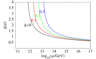
(b)

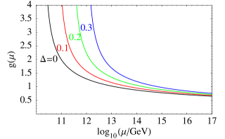
Figure 5.2: Running of the coupling constants of (a) $G_{\mathrm{hidden}}=\mathrm{SO}(8)$ (orbifold-mssm) and (b) $G_{\mathrm{hidden}}=\mathrm{SU}(4)$ [103] for different threshold corrections $\Delta$.

In section 5.2.3, we have seen that in an admissible vacuum configuration that preserves susy at high energies (as high as the string scale) the unbroken hidden sector is reduced to $G_{\mathrm{hidden}}=\mathrm{SO}(8)$. Furthermore, we observe that there are some $\boldsymbol{8}$–plets in this sector (cf. table 5.1). These states can be split in two sets, which form mass terms independently (see table F.1). In the vacuum configuration (5.55), their mass matrices are given by

$$\begin{array}[]{ccc}\mathcal{M}_{ww}=\left(\begin{array}[]{ccccc}\widetilde{s}&\widetilde{s}^{5}&0&\widetilde{s}^{5}&\widetilde{s}^{5}\\ \widetilde{s}^{5}&\widetilde{s}&0&\widetilde{s}^{5}&\widetilde{s}^{5}\\ 0&0&0&\widetilde{s}^{3}&\widetilde{s}^{3}\\ \widetilde{s}^{5}&\widetilde{s}^{5}&\widetilde{s}^{3}&\widetilde{s}^{6}&\widetilde{s}^{6}\\ \widetilde{s}^{5}&\widetilde{s}^{5}&\widetilde{s}^{3}&\widetilde{s}^{6}&\widetilde{s}^{6}\end{array}\right),&&\mathcal{M}_{f\bar{f}}~{}=~{}\left(\begin{array}[]{cc}0&\widetilde{s}^{3}\\ 0&\widetilde{s}^{3}\end{array}\right)\;.\end{array}$$ (5.71)

The first of these matrices has maximal rank, but from the second matrix there is a pair $f,\bar{f}$ that stays massless up to energies lower than $M_{\mathrm{GUT}}$.

Let us proceed to compute the gravitino mass $m_{3/2}$. We will require the beta-coefficient that can be computed by

$$b^{\mathrm{SO}(2N)}_{0}~{}=~{}6\cdot(N-1)-\#(\boldsymbol{2N}\text{--plets})\,;$$ (5.72)

in our case it is $b_{0}^{\mathrm{SO}(8)}=16$. Therefore, with the realistic value for the stabilization of the dilaton, $\operatorname{Re}\langle S\rangle\approx 2$, we obtain from eq. (5.60)

$$\Lambda~{}\approx~{}M_{\mathrm{GUT}}e^{-\pi^{2}}\approx 10^{12}\text{ GeV}\,,$$ (5.73)

what in turn yields the gravitino mass $m_{3/2}\approx 1$ GeV. This scale is phenomenologically unacceptable because that scale has been already ruled out by experiment. However, as we mentioned before, threshold corrections can modify this scale. In fact, by using eqs. (5.59) and (5.70), we find that threshold corrections enhance the scale of gaugino condensation and, therefore, also the gravitino mass. In fig. (5.2) we present the running of the gauge coupling $g(\mu)$ for two different cases. Fig. (5.2)(a) illustrates the influence of different values of $\Delta$ on the behavior of the gauge coupling. We notice that for $\Delta=0$ we recover the result given in eq. (5.73) whereas for $\Delta=0.3$ the condensation scale becomes almost $10^{14}$ GeV. In fig. (5.2)(b), we compare our result with a case where the hidden sector has an $\mathrm{SU}(4)$ gauge group and no massless matter in that sector. We might say that the situation in $\mathrm{SO}(8)$ is somewhat better than in $\mathrm{SU}(4)$. However, we must recall that there are of course other factors that can affect our estimates. For example, we have not described precisely the mechanism to stabilize the dilaton. Further, we have used the symbol ‘$\approx$’ in many of our equations because those values are not precise. Therefore, in this study the most important result is that the scale of susy lies around the phenomenologically interesting interval.

5.3.2 susy Breakdown in the (Mini-)Landscape

After having examined some of the most important aspects of gaugino condensation, we would like to continue our study on the set of mssm-candidates obtained in the last chapter through a search guided by grand unification. We have found 196 orbifold models (cf. table 4.3) with the following properties:
.     $\bullet$ sm gauge group times additional gauge factors,
.     $\bullet$ nonanomalous hypercharge of the Georgi-Glashow type, i.e. consistent with gauge .coupling unification,
.     $\bullet$ three mssm matter generations plus vectorlike exotics,
.     $\bullet$ all vectorlike exotics are decoupled from the massless spectrum.
In order to save some computation time, we have imposed an additional constraint on the models. Namely, we have demanded one trilinear coupling of the type $q\,\ell\,\bar{u}$ which might be responsible for the heavy mass of the top quark. Although this condition is not arbitrary, it is also not imperative since a heavy top quark might also appear through alternative methods. However, for consistency, we will stick to that constraint in this section.

The strategy we have followed consists in first finding a set of mssm candidates and then studying common features that could lead to some sort of low–energy predictions. In this section, we concentrate on the question of susy breaking. Particularly, we would like to figure out whether our mssm candidates yield a reasonable scale of susy breaking via hidden sector gaugino condensation.

With that purpose, we will impose an additional criterion in our search

1. Select models where exotics decouple + gaugino condensation

At this step, we select models in which the decoupling of the sm exotic states is possible without breaking the largest gauge group in the hidden sector. We find that all or almost all of the matter states charged under this group also attain large masses which allow for spontaneous susy breaking via gaugino condensation.

Criterion $V^{\mathrm{SO}(10),1}$ $V^{\mathrm{SO}(10),2}$ $V^{\mathrm{E}_{6},1}$ $V^{\mathrm{E}_{6},2}$ ➆ heavy top 72 37 3 2 ➇ exotics decouple at order 8 56 32 3 2 ➈ exotics decouple + gaugino condensation 47 25 3 2

Table 5.2: A subset of the mssm candidates.

Among the models satisfying all our criteria, ➁–➈, we consider the most promising mssm candidates. Our results are presented in table 5.2. We find it remarkable that out of ${\mathcal{O}}(10^{4})$ inequivalent models, ${\mathcal{O}}(10^{2})$ pass all of our requirements, including a hidden sector that allows susy breaking. In this sense, the region of the heterotic landscape endowed with local $\mathrm{SO}(10)$ and $\mathrm{E}_{6}$ guts is particularly attractive.

A comment is in order. We impose by hand the requirement that gaugino condensation be allowed. By assigning vevs to all sm singlets, i.e. without verifying explicitly $D$– and $F$–flatness, the hidden sector gauge group is broken by matter vevs charged under this group. Similarly, the sm gauge group is broken in more general “vacuum” configurations where many other fields can also acquire vevs. Clearly, most of the string landscape is not relevant to our physical world. It is only possible to obtain useful predictions from the landscape once certain criteria are imposed. Here we require that gaugino condensation be allowed so that susy can be broken. Since the largest hidden sector group factor would dominate susy breaking, we focus on vacua in which this factor is preserved by matter vevs. Within the set of our promising models, we can now study predictions for the scale of susy breaking.

Our mssm candidates have the necessary ingredients for supersymmetry breaking via gaugino condensation in the hidden sector. In particular, they contain nonabelian gauge groups under which little or no matter states are charged. The corresponding gauge interactions become strong at some intermediate scale which can lead to spontaneous supersymmetry breakdown. The specifics depend on the moduli stabilization mechanism, but the main features such as the scale of supersymmetry breaking hold more generally. In particular, the gravitino mass is given by

$$m_{3/2}\approx\frac{\Lambda^{3}}{M_{\mathrm{Pl}}^{2}}\;,$$ (5.74)

while the proportionality constant is model-dependent.

The gaugino condensation scale $\Lambda$ is given by the renormalization group invariant scale of the condensing gauge group,

$$\Lambda~{}\sim~{}M_{\mathrm{GUT}}\,\exp\left\{-\frac{1}{2\beta}\,\frac{1}{g^{2}(M_{\mathrm{GUT}})}\right\}\,.$$ (5.75)

With an appropriate mechanism, the dilaton can be stabilized at a realistic value $\operatorname{Re}\langle S\rangle\approx 2$ while breaking susy. As already mentioned, we see that for $\Lambda\sim 10^{13}$ GeV, the gravitino mass lies in the TeV range which is favored by phenomenology. susy breaking is communicated to the observable sector by gravity [123].

(a)

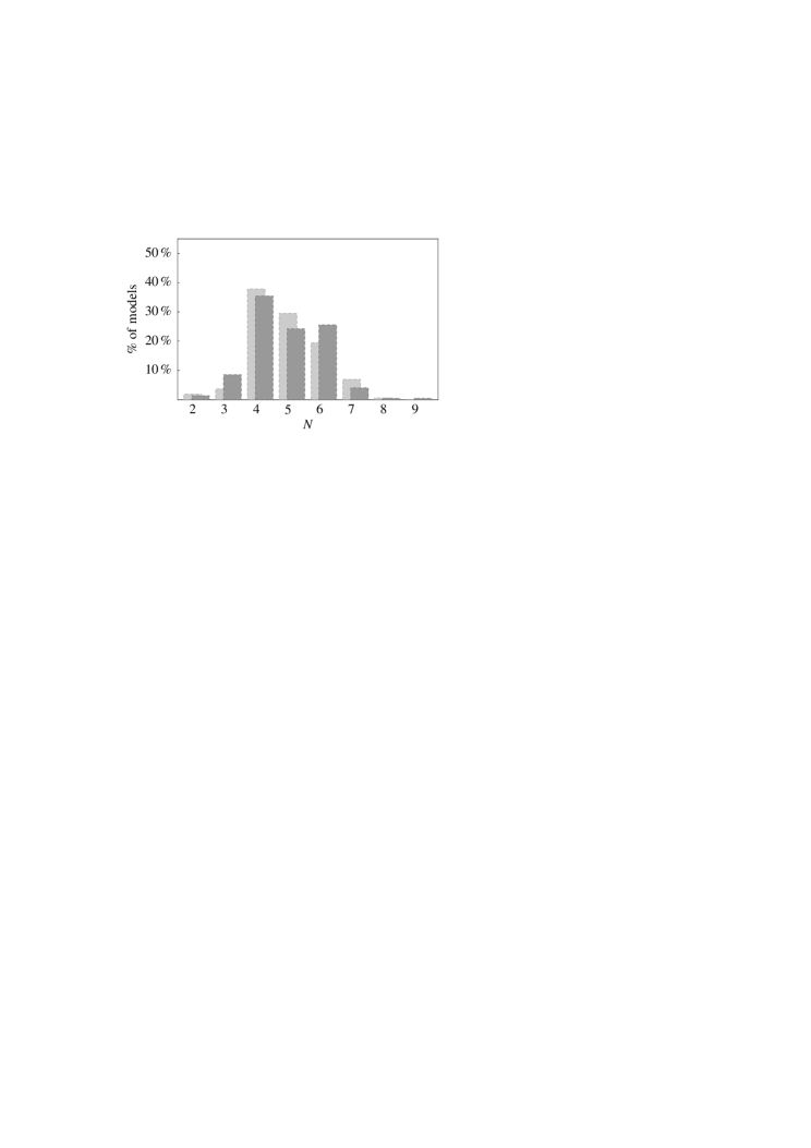
(b)

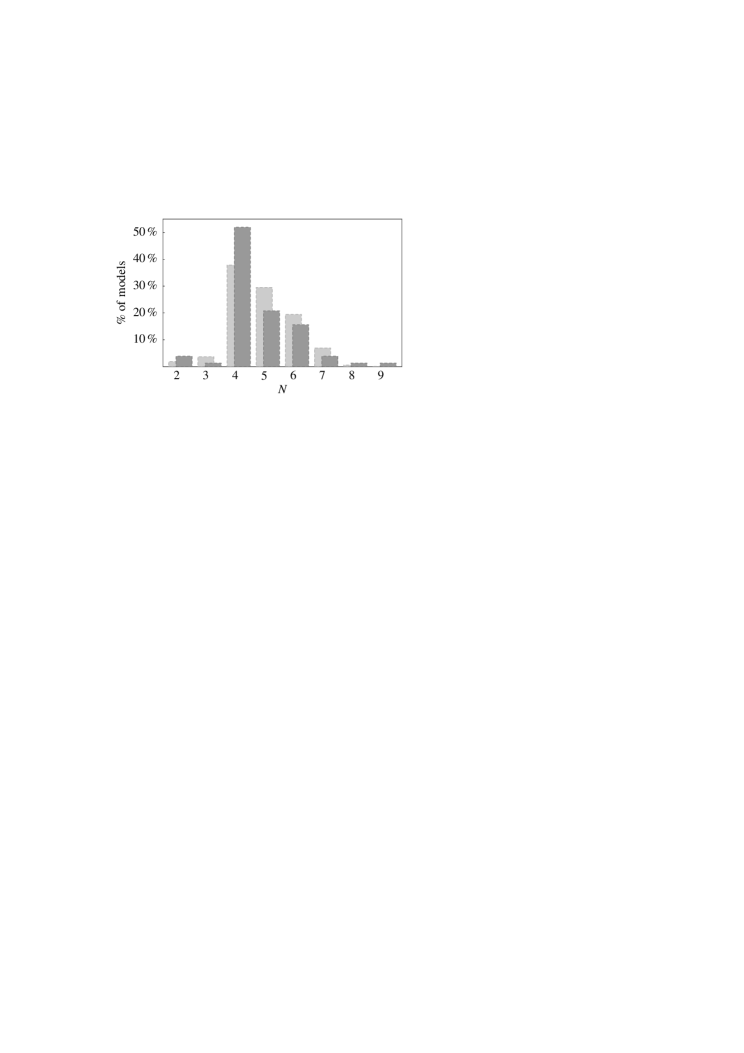
Figure 5.3: (a) Number of models vs. the size of largest gauge group in the hidden sector. $N$ labels $\mathrm{SU}(N)$, $\mathrm{SO}(2N)$, $\mathrm{E}_{N}$ groups. The background corresponds to step ➁, while the foreground corresponds to step ➅ (see table 4.2). (b) As before, but with models of step ➇ at the foreground.

In fig. 5.3(a), we display the frequency of occurrence of various gauge groups in the hidden sector. The preferred size ($N$) of the gauge groups depends on the conditions imposed on the spectrum. When all inequivalent models with two Wilson lines are considered, $N=4,5,6$ appear with similar likelihood and $N=4$ is somewhat preferred. If we require the massless spectrum to be the mssm + vectorlike matter, the fractions of models with $N=4,5,6$ become even closer. However, if we further require a heavy top quark and the decoupling of exotics at order eight, $N=4$ is clearly preferred (figure 5.3(b)). In this case, $\mathrm{SU}(4)$ and $\mathrm{SO}(8)$ provide the dominant contribution. Since all or almost all matter charged under these groups is decoupled, this leads to gaugino condensation at an intermediate scale. Possible scales of gaugino condensation are shown in fig. 5.4.

The correlation between the observable and hidden sectors comes about for a few reasons. First, it is due to modular invariance which ties the gauge shifts and Wilson lines in the two sectors. Second, the gauge shifts and Wilson lines in the hidden sector affect properties of the massless spectrum, for instance, through the masslessness equations.

We see that among the promising models, just as in the orbifold-mssm presented in section 5.3.1, intermediate scale supersymmetry breaking is preferred. The underlying reason is that realistic spectra require complicated Wilson lines, which break the hidden sector gauge group. The surviving gauge factors are neither too big (unlike in Calabi–Yau compactifications with the standard embedding) nor too small.

There are significant uncertainties in the estimation of the supersymmetry-breaking scale. First, the identification of $\Lambda$ with the renormalization group invariant scale is not precise. A factor of a few uncertainty in this relation leads to two orders of magnitude uncertainty in $m_{3/2}$. Also, there could be significant string threshold corrections which can affect the estimate although we see from fig. (5.2) that threshold corrections might enhance the scale of susy breaking. Thus, the resulting “prediction” for the superpartner masses should be understood within 2-3 orders of magnitude.

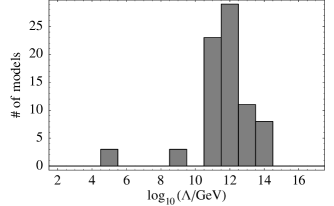
Figure 5.4: Number of models vs. scale of gaugino condensation.

5.4 $\boldsymbol{R}$-Parity and Proton Decay

An essential property of the mssm that a realistic model must exhibit is $R$-parity. This has the advantage of greatly reducing the number of arbitrary parameters in the superpotential, forbidding dimension three and four baryon or lepton number violating operators, and preserving a viable dark matter candidate, i.e. the LSP. However, obtaining a conserved $R$-parity in string constructions sets frequently an insurmountable hurdle, which must however be overcome in order to reach the mssm.

Our strategy for accomplishing this is, in principle, quite simple. We identify first a $\mathrm{U}(1)_{B\!-\!L}$ gauge symmetry and then give vevs to some sm singlets that break $\mathrm{U}(1)_{B\!-\!L}$ to the discrete subgroup

$$\mathbbm{Z}_{2}^{\mathcal{M}}~{}:~{}(-1)^{3(B\!-\!L)}\,.$$ (5.76)

This unbroken discrete symmetry is the so-called family reflection symmetry or matter parity [143], which, due to its properties, can be considered an $R$-parity. This is a global $\mathbbm{Z}_{2}$ symmetry which is even on the Higgs doublets and odd on all sm quark and lepton fields. Further, it forbids dangerous baryon or lepton number violating operators of dimension three and four:

$$\overline{u}\,\overline{d}\,\overline{d}\;,\quad q\,\overline{d}\,\ell\;,\quad\ell\,\ell\,\overline{e}\quad\text{and}\quad\ell\,h_{u}\;.$$ (5.77)

On the other hand, it allows quark and lepton Yukawa couplings as well as the Majorana neutrino mass operator $\bar{\nu}\bar{\nu}$. However, there are certain dimension five operators that are allowed by this symmetry:

$$\kappa^{(1)}_{ijkl}q_{i}\,q_{j}\,q_{k}\,\ell_{l}\,,\qquad\kappa^{(2)}_{ijkl}\bar{u}_{i}\,\bar{u}_{j}\,\bar{d}_{k}\,\bar{e}_{l}\,,$$ (5.78)

which can induce proton decay (see fig. (5.4)). $\kappa^{(1)}$ and $\kappa^{(2)}$ are coupling constants. In the mssm  $\kappa^{(1)}$ is constrained by [144]

$$\frac{\kappa^{(1)}_{1121}}{\Lambda^{cut}}\approx\frac{\kappa^{(1)}_{1122}}{\Lambda^{cut}}\lesssim 16\pi^{2}\frac{M_{\textrm{SUSY}}}{M_{\textrm{GUT}}^{2}}$$ (5.79)

and $\kappa^{(2)}$ can take arbitrary values as long as they are consistent with perturbation theory. Here, $\Lambda^{cut}$ denotes an intermediate cut-off scale and $M_{\textrm{SUSY}}\approx 10^{4}$ GeV is the scale at which susy is supposed to break.

Figure 5.5: Possible contribution to proton decay, involving the dimension five operator $q\,q\,q\,\ell$. The proton decays as $p\rightarrow K^{+}\bar{\nu}\text{ or }\pi^{+}\bar{\nu}$.

We build the $\mathrm{U}(1)_{B\!-\!L}$ symmetry as a superposition of all gauge $\mathrm{U}(1)$’s of the mssm candidates excepting the anomalous one. In our mssm candidates, a natural choice for the generator of $\mathrm{U}(1)_{B\!-\!L}$ follows from the standard breaking

$$\mathrm{SO}(10)\rightarrow\mathrm{SU}(5)\times\mathrm{U}(1)_{X}\rightarrow G_{SM}\times\mathrm{U}(1)_{X}\,,$$ (5.80)

where the generators of hypercharge and $B-L$ are given by

$$\mathsf{t}_{Y} = \left(-\frac{1}{2},\,-\frac{1}{2},\,\frac{1}{3},\,\frac{1}{3},\,\frac{1}{3}\right),\,$$ (5.81)

$$\mathsf{t}_{B\!-\!L} = \frac{2}{5}\left(2\,\mathsf{t}_{Y}+\mathsf{t}_{X}\right)~{}=~{}\left(0,\,0,\,\frac{2}{3},\,\frac{2}{3},\,\frac{2}{3}\right)$$ (5.82)

with $\mathsf{t}_{X}=(1^{5})$ generating the additional $\mathrm{U}(1)_{X}$. Under these symmetries, including $\mathrm{SU}(3)_{c}\times\mathrm{SU}(2)_{L}$, an mssm matter generation has the quantum numbers

$$\begin{array}[]{rcccccc}\boldsymbol{16}~{}=&(\boldsymbol{3},\boldsymbol{2})_{\frac{1}{6},\frac{1}{3}}+&(\boldsymbol{\overline{3}},\boldsymbol{1})_{-\frac{2}{3},-\frac{1}{3}}+&(\boldsymbol{\overline{3}},\boldsymbol{1})_{\frac{1}{3},-\frac{1}{3}}+&(\boldsymbol{1},\boldsymbol{2})_{-\frac{1}{2},-1}+&(\boldsymbol{1},\boldsymbol{1})_{1,1}+&(\boldsymbol{1},\boldsymbol{1})_{0,1}\,,\\[5.69054pt] &q&\bar{u}&\bar{d}&\ell&\bar{e}&\bar{\nu}\end{array}$$ (5.83)

where the subscripts denote hypercharge and $B\!-\!L$ charge, respectively. Further, the Higgs doublets $\phi$ and $\bar{\phi}$ have $\mathrm{U}(1)$ charges $(-1/2,0)$ and $(1/2,0)$, respectively.

Unfortunately, the symmetry generated by $\mathsf{t}_{B\!-\!L}$ mixes with $\mathrm{U}(1)_{A}$ in our mssm candidates and is, hence, ruled out. We have to search for a different “suitable” definition of $\mathrm{U}(1)_{B\!-\!L}$ which has to satisfy two conditions:
.    (i)  it must assign the standard $B\!-\!L$ charges, eq. (5.83) to all sm particles (including a pair of Higgs fields), and
.    (ii) it must give most sm singlets a value that satisfies $3(B\!-\!L)=0\mod 2$.

Condition (i) is clear, but the second condition requires some argumentation. Firstly, sm singlets with charges $3(B\!-\!L)=0\mod 2$ can obtain vevs for decoupling exotics, as well as giving effective quark and lepton Yukawa couplings. Secondly, if there are some singlets (let us call them $\chi_{i}$) satisfying $3(B\!-\!L)=0\mod 2$ and with nontrivial $B\!-\!L$ charge, they will break $\mathrm{U}(1)_{B\!-\!L}$, but will leave the $R$-parity, $\mathbbm{Z}_{2}^{\mathcal{M}}$, unbroken. Moreover, note that if singlets with $3(B\!-\!L)=1\mod 2$ develop nonvanishing vevs, $R$-parity is broken and dimension four baryon/lepton number violating operators are typically generated. We would like to remark that this approach to get $R$-parity is not unique. Alternatives arise from considering other internal symmetries, such as R-charge conservation (inherited from Lorentz invariance in ten dimensions) [112] or $T$–duality [145].

Searching for generators of $\mathrm{U}(1)_{B\!-\!L}$ is not difficult, but quite cumbersome. One has to express $\mathsf{t}_{B\!-\!L}$ as a superposition of all $\mathrm{U}(1)$’s, excepting the anomalous $\mathrm{U}(1)$,

$$\mathsf{t}_{B\!-\!L}=\sum_{i\neq A}x_{i}\mathsf{t}_{i}\,,$$ (5.84)

and solve (non)linear equations on the real parameters $x_{i}$ guaranteeing that the conditions (i) and (ii) explained above be fulfilled. The precise description of the method is provided in appendix D of ref. [53].

5.4.1 Supersymmetric mssm Candidates

Before going any further, there is a question that we have to clarify. In section 4.4, it was assumed that all sm singlets can acquire vevs. Nevertheless, we have learnt in section 5.2 a strategy to identify those singlets which admit a nonzero vev in a consistent supersymmetric vacuum. In the present case, since $B\!-\!L$ must be broken spontaneously, it results impossible to postpone the task of verifying $D$–flatness any longer.

$V^{\mathrm{SO}(10),1}$ $V^{\mathrm{SO}(10),2}$ Criterion ➆ ➆ ➆ ➆ ➅ spectrum $=$ 3 generations $+$ vectorlike 72 56 37 53 ➇ exotics decouple at order 8 56 50 32 53 ➇’ exotics decouple in susy configurations 55 50 32 53

Table 5.3: A subset of the mssm candidates. The number of models with “heavy top” are listed under ➆. ➆ denotes no “heavy top”. Only in one model, it was not possible to find a supersymmetric vacuum configuration where all exotics decouple.

Let us focus on the models based on the shifts $V^{\mathrm{SO}(10),1}$ and $V^{\mathrm{SO}(10),2}$, that is, in those that concentrate most promising models. According to our previous discussion, all we have to do is to verify whether there exist holomorphic invariant monomials (HIMs) with net negative anomalous charge. All fields entering the monomials are allowed to attain nonvanishing vevs and, therefore, contribute to the masses of the exotics.

We recall our results from chapter 4 and complement them with our new findings in table 5.3. In particular, observe that we have incorporated the nontrivial criterion ➇’. We have verified that all vectorlike exotics acquire large masses. These results are crucial for the discussion on breaking of $\mathrm{U}(1)_{B\!-\!L}$.

Notice that we have not discussed $F$–flatness or any other additional constraint (e.g. $\langle W\rangle=0$). As we mentioned in section 5.2, the reason is that other conditions are not relevant since they depend on technical particularities of the models, such as the order of the perturbative potential at hand. On the other hand, we do not have any prescription to write the full superpotential including all possible nonperturbative contributions. Additionally, we have shown that once one has found a $D$–flat configuration, it is always possible to find a nontrivial solution to the $F$–term equations.

5.4.2 $\boldsymbol{R}$-Parity Invariant mssm Candidates

For simplicity, we focus here only on those models from table 5.3 with a cubic top Yukawa coupling, that is, on those 55+32 mssm candidates satisfying simultaneously criteria ➆ and ➇’.

We notice that the shift $V^{\mathrm{SO}(10),1}$ seems still to be more promising in comparison to $V^{\mathrm{SO}(10),2}$. With our method, we find that 34 of the 55 (5 of the 32) mssm candidates from the first (second) shift vector admit nonanomalous definitions of $B\!-\!L$ . Each model, nevertheless, correspond to a big family of configurations with distinct acceptable $\mathrm{U}(1)_{B\!-\!L}$ symmetries. There are two reason for this to happen:

$\bullet$ In many cases there are vectorlike exotics with sm gauge charges identical to those of quarks and leptons. Further, without $B\!-\!L$ , each lepton doublet $\ell$ could very well be a Higgs boson $\phi$. Thus there are different ways to choose which of these states have standard $B\!-\!L$  charges. Each choice can lead to a different (and nonanomalous) definition of $B\!-\!L$ .

$\bullet$ For each choice of sm particles above, there may be more than one $B\!-\!L$ definition. The system of equations that determine the values of the variables $x_{i}$ in eq. (5.84) might be underconstrained. Therefore, in some cases, there are (continuous) families of $B\!-\!L$ generators (i.e. some of the $x_{i}$’s are free or fulfill equations with an undetermined number of solutions).

These ambiguities, although disturbing at first sight, might also be considered a rich source of new physics. However, it is clear that we need to implement new criteria in order to reduce the number of $B\!-\!L$ configurations. We require the presence of sm singlets with charges $B\!-\!L=0,\pm 2,\pm 2/3,\pm 2/5,\ldots,\pm 6/7$ in the spectrum. Configurations with singlets having $B\!-\!L$ charges consistent with $3(B\!-\!L)=0\mod 2$, but different from the values just mentioned are automatically disregarded.

Including only these possibilities, we find 3447 (144) consistent $B\!-\!L$ generators from the first (second) $\mathrm{SO}(10)$ shifts. The question is now whether all these configurations are inequivalent or not. It can be argued that, if one considers one single model (shift vector $+$ Wilson lines + hypercharge generator) with several $B\!-\!L$ configurations, we could distinguish the inequivalent configurations by comparing the sets of sm singlets with charges fulfilling $3(B\!-\!L)=0\mod 2$. If these sets (and not the charges) coincide in two models, one might state that they are equivalent and, thus, that one of them can be ignored. This is indeed the approach we follow.

In this approach, we find that there are “only” 85 (8) inequivalent $B\!-\!L$ configurations from $V^{\mathrm{SO}(10),1}$ ($V^{\mathrm{SO}(10),2}$). Further, as we are interested in models containing solely the sm gauge group times a hidden sector for gaugino condensation, one can verify whether all extra unbroken $\mathrm{U}(1)$’s break when fields with proper $B\!-\!L$ charges attain vevs. Requiring the absence of extra unbroken $\mathrm{U}(1)$’s reduces this set to 42 (0) acceptable configurations. Finally, demanding that all exotics decouple along $D$–flat directions leads to 15 (0) acceptable solutions with an exact low energy $R$-parity. We list the corresponding shifts, Wilson lines and generators of hypercharge and $B\!-\!L$  in table LABEL:tab:NiceBmLModels. These input parameters can be used to determine all other properties of the models.

This result is specific to our $(B\!-\!L)$-based strategy and we expect, in general, more acceptable models to exist. We point out that there is a big uncertainty in this number and, therefore, it should be taken as a lower bound.

5.4.3 $\boldsymbol{R}$-Parity in the Orbifold-mssm

The orbifold-mssm allows us to define a suitable $B\!-\!L$ generator which leads to the standard charges for the sm matter, eq. (5.83). The generator is given by

$$\mathsf{t}_{B\!-\!L}~{}=~{}\left(-1,\,-1,\,0,\,0,\,0,\,\tfrac{2}{3},\,\tfrac{2}{3},\,\tfrac{2}{3}\right)\left(-2x+\tfrac{1}{2},\,-\tfrac{1}{2},\,0,\,-x,\,-x,\,0,\,0,\,0\right)\;,$$ (5.85)

with arbitrary $x$. Let us take $x=\frac{1}{2}$. Then the $B\!-\!L$ generator we shall use is

$$\mathsf{t}_{B-L}~{}=~{}\left(-1,-1,0,0,0,\tfrac{2}{3},\tfrac{2}{3},\tfrac{2}{3}\right)\,,\left(-\tfrac{1}{2},-\tfrac{1}{2},0,-\tfrac{1}{2},-\tfrac{1}{2},0,0,0\right)\;.$$ (5.86)

An interesting feature is that the spectrum contains a pair of fields with $B\!-\!L$ charges $\pm 2$, so that, if the $B\!-\!L$ gauge symmetry is broken by vevs of these fields, the matter parity $(-1)^{3(B\!-\!L)}$ is conserved and proton decay due to dimension three and four operators is suppressed. In table F.1, we have summarized the matter spectrum of the model. Since now we include $B\!-\!L$ , we can now distinguish between fields with identical sm quantum numbers; in particular, we can distinguish now between Higgs and lepton doublets.

The vacuum configuration (5.55) is still admissible in presence of $\mathrm{U}(1)_{B\!-\!L}$. In this configuration, sm singlets with $B\!-\!L$  charges $\pm 2$, labeled $\chi_{1}\equiv s^{0}_{1}$ and $\chi_{2}\equiv s^{0}_{2}$, attain nonzero vevs and thus break $B\!-\!L$ by two units, such that, e.g. particles with $B\!-\!L$ charge $1$ are equivalent to particles with $B\!-\!L$ charge equal to $-1$. This example applies to the right–handed neutrinos to be studied in the next section.

Let us now proceed to enumerate some of the properties that the orbifold-mssm acquires after breaking $B\!-\!L$.

Absence of proton decay operators of dimension three and four. This is, of course, not surprising since we have imposed $B\!-\!L$ just to avoid these operators.

Cancellation of the $\boldsymbol{\mu}$–term. The Higgs mass terms are

$$\bar{\phi}_{i}\,(\mathcal{M}_{\bar{\phi}\phi})_{ij}\,\phi_{j}\;,\quad\text{where}\quad\mathcal{M}_{\bar{\phi}\phi}~{}=~{}\left(\begin{array}[]{cccc}\widetilde{s}^{4}&0&0&\widetilde{s}\\ \widetilde{s}&\widetilde{s}^{3}&\widetilde{s}^{3}&\widetilde{s}^{6}\\ \widetilde{s}^{5}&0&0&\widetilde{s}^{3}\\ \widetilde{s}&0&0&\widetilde{s}^{3}\end{array}\right)\;.$$ (5.87)

The up-type Higgs $h_{u}$ is a linear combination of $\bar{\phi}_{1}$, $\bar{\phi}_{3}$ and $\bar{\phi}_{4}$,

$$h_{u}~{}\sim~{}\widetilde{s}^{2}\bar{\phi}_{1}+\bar{\phi}_{3}+\widetilde{s}^{4}\,\bar{\phi}_{4}\;,$$ (5.88)

while the down-type Higgs is composed out of $\phi_{2}$ and $\phi_{3}$,

$$h_{d}~{}\sim~{}\,\phi_{2}+\phi_{3}\;.$$ (5.89)

Let us remark that this spoils our argument about the existence of “heavy top”.

Notice that in this vacuum configuration the $\mu$–term, being defined as the smallest eigenvalue of $\mathcal{M}_{\bar{\phi}\phi}$,

$$\mu~{}=~{}\left.\frac{\partial^{2}W}{\partial h_{d}\,\partial h_{u}}\right|_{h_{u}=h_{d}=0}\,,$$ (5.90)

vanishes term by term up to order $\widetilde{s}^{6}$, at which we work. This is a way to deal with the supersymmetric $\mu$–problem.

Charged fermion Yukawa matrices. The up-Higgs Yukawa couplings decompose into

$$W_{\mathrm{Yukawa}}~{}\supset~{}\sum\limits_{k=1}^{4}(Y_{u})_{ij}^{(k)}\,q_{i}\,\bar{u}_{j}\,\bar{\phi}_{k}\,,$$ (5.91)

where the matrices $Y_{u}^{(i)}$ are given in appendix F. Thus, the physical $3\times 3$ up-Higgs Yukawa matrix is

$$Y_{u}~{}\sim~{}\widetilde{s}^{2}\,Y_{u}^{(1)}+Y_{u}^{(3)}+\widetilde{s}^{4}\,Y_{u}^{(4)}~{}=~{}\left(\begin{array}[]{ccc}0&0&\widetilde{s}^{8}\\ 0&0&\widetilde{s}^{8}\\ \widetilde{s}^{5}&\widetilde{s}^{5}&\widetilde{s}^{2}\end{array}\right)\,.$$ (5.92)

Note that due to the Higgs mixing the top quark Yukawa coupling for this vacuum configuration is given by $\widetilde{s}^{2}$. Therefore, the corresponding $\widetilde{s}$ vevs are required to be quite large.

The down-Higgs Yukawa couplings decompose into

$$W_{\mathrm{Yukawa}}~{}\supset~{}\sum\limits_{k=1}^{4}(Y_{d})_{ij}^{(k)}\,q_{i}\,\bar{d}_{j}\,\phi_{k}\,,$$ (5.93)

where again the Yukawa matrices are provided in appendix F.

The physical $3\times 3$ down-Higgs Yukawa matrix emerges by integrating out a pair of vectorlike $d-$ and $\bar{d}-$quarks,

$$Y_{d}~{}=~{}\left(\begin{array}[]{ccc}1&\widetilde{s}^{3}&0\\ 1&\widetilde{s}^{3}&0\\ \widetilde{s}&\widetilde{s}^{4}&0\end{array}\right)\,.$$ (5.94)

We note that both the up and down quarks are massless at order six in sm singlets. However, we have checked that the up quark becomes massive at order seven and the down quark gets a mass at order eight.

Analogously, the physical $3\times 3$ matrix emerges by integrating out a pair of vector-like $\ell-$ and $\bar{\ell}-$leptons,

$$Y_{e}~{}=~{}\left(\begin{array}[]{ccc}1&1&\widetilde{s}\\ \widetilde{s}&\widetilde{s}&\widetilde{s}^{2}\\ 0&0&\widetilde{s}^{6}\\ \end{array}\right)\,.$$ (5.95)

Dimension five baryon and lepton number violating operators. We have looked for effective dimension five baryon and lepton number violating operators in this model. We find that to order $\tilde{s}^{6}$ no such operators exist. However, these operators can be generated once the exotics $\delta_{i},\ \bar{\delta}_{i}$ are integrated out. Fortunately, a clever choice of vevs for the fields $\{\widetilde{s}_{i}\}$ can guarantee sufficient suppression of all induced $q\,q\,q\,\ell$ operators, consistent with current bounds on proton decay, eq. (5.79).

$\boldsymbol{\mu}$–term and Minkowski space. In many mssm candidates, the $\mu$–term is identified with the singlet-superpotential, $W(\widetilde{s}_{i})$. This occurs if the product of the Higgs fields $h_{u}\,h_{d}$ fulfills trivially all selection rules. In such models, one can show that if $W(\widetilde{s}_{i})$ is endowed with an approximate $R$-symmetry, it follows directly that $\mu=\langle W(\widetilde{s}_{j})\rangle=0$ and, in the context of supergravity, also $D_{i}W=0$ [146]. That is, one obtains a supersymmetric Minkowski vacuum. Since string theories do not admit global symmetries at all orders in the superpotential, the $R$-symmetry of the superpotential is broken at higher orders in the superpotential. This implies that the effective $\mu$-term is highly suppressed.

Unfortunately, this is not the case in our orbifold-mssm. The problem is that $h_{u}\,h_{d}$ does not satisfy all selection rules, which follows from the fact that in the orbifold-mssm there are four Higgs pairs and they mix. The fact that we do obtain a Minkowski vacuum in this model is therefore not linked to a symmetry of the theory. This has the consequence that supergravity may lead to a deep anti-De Sitter vacuum.

Further details of the orbifold-mssm regarding the effect of our $B\!-\!L$ choice on the neutrino masses will be discussed in the next section. The detailed mass matrices are displayed in appendix F.

5.5 Neutrino Masses

The seesaw mechanism [147, 148, 149] is perhaps the most attractive way to explain the smallness of the neutrino masses. Its essential ingredients are heavy Majorana neutrinos and their Yukawa couplings to the left–handed neutrinos. The supersymmetric seesaw mechanism is described by the superpotential

$$W~{}=~{}Y_{\nu}^{ij}\,\bar{\phi}\,\ell_{i}\,N_{j}+\frac{1}{2}M_{jk}N_{j}\,N_{k}\;,$$ (5.96)

where $\bar{\phi}$ and $\ell_{i}$ ($i=1,2,3$) are the up–type Higgs and lepton doublets, and $N_{j}$ ($1\leq j\leq n$) are some heavy standard model singlets. At low energies, this leads to three light neutrinos with masses of order $(Y_{\nu}\,\langle\bar{\phi}\rangle)^{2}/M$, where $Y_{\nu}$ and $M$ represent typical values of $Y_{\nu}^{ij}$ and $M_{jk}$, respectively. For $Y_{\nu}\sim 1$ and $M\sim 10^{16}\,\mathrm{GeV}$, one has $m_{\nu}\sim 10^{-3}\mathrm{eV}$. The scales of the atmospheric and solar neutrino oscillations, [150]

$$\sqrt{\Delta m^{2}_{\mathrm{atm}}}\simeq 0.04\,\mathrm{eV}\,,\qquad\sqrt{\Delta m^{2}_{\mathrm{sol}}}\simeq 0.008\,\mathrm{eV}\,,$$ (5.97)

are suspiciously close to this scale. This hints at gut structures behind the seesaw.

In conventional guts, $N_{j}$ are members of gut matter multiplets, e.g. a $\boldsymbol{16}$–plet of $\mathrm{SO}(10)$, and $M_{jk}$ are related to a vev of a large gut representation, e.g. a $\overline{\boldsymbol{126}}$–plet of $\mathrm{SO}(10)$. In this case the Majorana mass terms originate from the coupling $\boldsymbol{16}\,\boldsymbol{16}\,\overline{\boldsymbol{126}}$ (cf. e.g. [151]).

5.5.1 Seesaw Mechanism with Several Neutrinos

Even though in our scheme we have local guts, the Yukawa couplings do not necessarily preserve the symmetry of these guts. The symmetry of the nonlocal coupling in ten dimensions is an intersection of the local gauge groups at the vertices. This implies, for example, that the Majorana mass terms for the neutrino components of the $\boldsymbol{16}$–plets can originate from the coupling

$$\nu_{\boldsymbol{16}}\times\nu_{\boldsymbol{16}}\times(\text{{\sc sm}\ singlets})\;,$$ (5.98)

where the singlets belong neither to $\accentset{(-\!\!-\!\!-)}{\boldsymbol{16}}$ nor to $\accentset{(-\!\!-\!\!-\!\!-\!\!-)}{\boldsymbol{126}}$ of $\mathrm{SO}(10)$.

Furthermore, any sm singlet can play the role of the right–handed neutrino as long as it has a Yukawa coupling to the lepton doublets and a large Majorana mass. These are abundant in orbifold models and typical models contain $\mathcal{O}(100)$ such singlets.

mssm candidates contain an anomalous $\mathrm{U}(1)$ which induces the FI $D$-term,

$$D_{A}~{}=~{}\frac{g\,M_{\mathrm{Pl}}^{2}}{192\pi^{2}}~{}\operatorname{tr}\mathsf{t}_{A}+\sum_{i}q_{i}\,|\phi_{i}|^{2}\;,$$ (5.99)

where $\mathsf{t}_{A}$ is the anomalous $\mathrm{U}(1)$ generator, $q_{i}$ are the anomalous charges of fields $\phi_{i}$ and $g$ is the gauge coupling. This triggers spontaneous gauge symmetry breaking while preserving supersymmetry [80]. Some of the fields charged under the anomalous $\mathrm{U}(1)$ (and, in addition, under other gauge groups) develop nonzero vevs thereby reducing gauge symmetry. The scale of these vevs is set by the FI term which is somewhat below the string scale. This eventually determines the seesaw scale. In general, any sm singlets can get large vevs as long as it is consistent with supersymmetry, and one can obtain the standard model gauge symmetry times that of the hidden sector,

$$\mathcal{G}_{4D}~{}\longrightarrow~{}G_{SM}\times G_{\mathrm{hidden}}\;.$$ (5.100)

The singlet vevs are not necessarily associated with flat directions in the field space and generally correspond to isolated solutions to supersymmetry equations [103]. The hidden matter gauge group $G_{\mathrm{hidden}}$ can be responsible for spontaneous supersymmetry breaking. In fact, within the class of models with the mssm spectrum, gaugino condensation in the hidden sector favors TeV–scale soft masses for the observable fields, as we have seen in section 5.3.2.

The nonzero singlet vevs lead to the mass terms for the vectorlike states,

$$W~{}=~{}x_{i}\,\bar{x}_{j}\,\langle s_{a}\,s_{b}\,\dots\rangle\;,$$ (5.101)

where $x_{i},\bar{x}_{j}$ are the vectorlike exotics and $\langle s_{k}\rangle$ are the sm singlet vevs in string units. Such a coupling must be consistent with string selection rules. In section 5.4, it has been shown that many $\mathbbm{Z}_{6}$-II models satisfy this requirement and all of the vectorlike exotics can be decoupled. This results in the mssm spectrum at low energies.

Similarly, the singlet vevs induce “Majorana” mass terms for the sm singlets as well as the neutrino Yukawa couplings of eq. (5.96),

$$M_{ij}\sim\langle s_{a}\,s_{b}\,\dots\rangle~{}~{},~{}~{}Y_{\nu}^{ij}\sim\langle s_{\alpha}\,s_{\beta}\,\dots\rangle~{},$$ (5.102)

as long as it is consistent with string selection rules.

Identification of right–handed neutrinos is intimately related to the issue of baryon/lepton number violation. In generic vacua, any sm singlet can play the role of the right–handed neutrino. However, such vacua also suffer from excessive $R$-parity violating interactions. The simplest way to suppress these interactions is to identify a $B\!-\!L$ gauge symmetry and enforce either its approximate conservation or conservation of its discrete (matter parity) subgroup. In local guts, the $B\!-\!L$ generator resembles the standard gut $B\!-\!L$, but also requires extra $\mathrm{U}(1)$ components beyond $\mathrm{SO}(10)$. It is nonanomalous and produces the standard $B\!-\!L$ charges for the sm matter. If $B\!-\!L$ is broken by vevs of fields carrying even charges under $B\!-\!L$, the matter parity $(-1)^{3(B\!-\!L)}$ is conserved. This forbids dangerous $R$-parity violating interactions and requires the right-handed neutrino to carry the charge $q_{B\!-\!L}=\pm 1$. Another possibility is that $\mathrm{U}(1)_{B\!-\!L}$ is broken at an intermediate scale $M_{B\!-\!L}$ such that all $R$-parity violating couplings are suppressed by $M_{B\!-\!L}/M_{\mathrm{Pl}}$. In this case, Majorana mass terms for the right–handed neutrinos are allowed only upon $B\!-\!L$ breaking, which lowers the seesaw scale to intermediate energies. In what follows, we consider these possibilities in specific heterotic orbifold models.

5.5.2 Seesaw Mechanism on the Orbifold-mssm

The $B\!-\!L$ generator is identified with

$$\mathsf{t}_{B\!-\!L}~{}=~{}\left(-1,-1,0,0,0,\tfrac{2}{3},\tfrac{2}{3},\tfrac{2}{3}\right)\,\left(-\tfrac{1}{2},-\tfrac{1}{2},0,-\tfrac{1}{2},-\tfrac{1}{2},0,0,0\right)\;.$$ (5.103)

In general supersymmetric configurations, many sm singlets get nonzero vevs. Choosing a subset of such singlets with 0 or $\pm 2$ $B\!-\!L$ charges, the unbroken gauge symmetry is

$$G_{\mathrm{SM}}\times G_{\mathrm{hidden}}\;,$$ (5.104)

where $G_{\mathrm{hidden}}=\mathrm{SO}(8)$, while all of the exotic states get large masses and decouple. This vacuum preserves the matter parity $(-1)^{3(B\!-\!L)}$.

We find that there are 39 right–handed neutrinos defined by $q_{B\!-\!L}=\pm 1$, two of which are members of the localized $\boldsymbol{16}$–plets. They have Yukawa couplings to the lepton doublets and large Majorana mass terms. We have calculated the $3\times 39$ Yukawa matrix $Y_{\nu}$ and $39\times 39$ Majorana mass matrix $M$ of eq. (5.96) up to order six in the singlet vevs. That is, for each matrix element, we have determined at which order in the superpotential a nonzero coupling is allowed by string selection rules. Each entry depends on the quantum numbers and the localization of the Majorana neutrinos, and involves products of different singlets and moduli-dependent Yukawa couplings. We then assume that the main hierarchy in these entries comes from products of singlet vevs so that these matrices can be treated as textures.

The effective mass matrix for the left–handed neutrinos,

$$M_{\mathrm{eff}}~{}=~{}-v_{u}^{2}\,Y_{\nu}\,M^{-1}\,Y_{\nu}^{T}$$ (5.105)

with $v_{u}$ being the up–type Higgs vev, can be represented by the texture

$$M_{\mathrm{eff}}~{}\sim~{}-\frac{v_{u}^{2}}{M_{*}}\left(\begin{matrix}1&s&s\\ s&s^{2}&s^{2}\\ s&s^{2}&s^{2}\end{matrix}\right)\;.$$ (5.106)

Here $s<1$ represents a generic singlet vev in string units and $M_{*}$ is the effective seesaw scale. $Y_{\nu}$ contains entries with powers of $s$ between 1 and 5, while the dependence of the eigenvalues of $M$ ranges from $s$ to $s^{8}$ (with no massless eigenstates at generic points in moduli space). This results in a strong $s$-dependence of the effective seesaw scale $M_{*}$. This scale is further suppressed by the large multiplicity of heavy singlets $N$, $M_{*}\propto N^{-x}$ with $0<x<2$. The value of $x$ depends on the texture. For example, when all the singlets contribute equally, $x=2$, whereas $x=0$ if only a fixed number of neutrinos have nonnegligible couplings. For the present model, we find

$$M_{*}~{}\sim~{}0.1\,s^{5}\,M_{\rm str}~{}\sim~{}10^{14}\,\mathrm{GeV}\;,$$ (5.107)

for the string scale $M_{\rm str}=2\cdot 10^{17}\,\mathrm{GeV}$ and $s\sim 0.3$. The obtained texture (5.106) is of course model dependent.

The corresponding charged lepton Yukawa matrix is of the form

$$Y_{e}~{}\sim~{}\left(\begin{matrix}1&1&c\\ c&c&c^{2}\\ 0&0&0\end{matrix}\right)\;,$$ (5.108)

where “0” denotes absence of the coupling up to order six in the singlet vevs $c$. Such zeros are expected to be filled in at higher orders. Here we are again using a single expansion parameter although in practice there are many variables.

These crude estimates show that reasonable fermion masses can in principle be obtained. Inserting order one coefficients in the textures, one finds that the eigenvalues scale as

$$m_{\nu_{i}}~{}\sim~{}(1,s^{2},s^{2})\,\frac{v_{u}^{2}}{M_{*}}\;,\quad m_{e_{i}}~{}\sim~{}(1,c,0)\,v_{d}\;,$$ (5.109)

where $v_{d}$ is the down–type Higgs vev. For $s\sim 0.3$ and $c\sim 0.1$ the textures reproduce roughly the observed lepton mass hierarchy. The above texture favors the normal neutrino mass hierarchy and can accommodate small and large mixing angles. Further details of the model are available in appendix F.

Chapter 6 Beyond the Mini-Landscape

We broaden our search of promising models. We drop the requirement of having a local $\mathrm{SO}(10)$ or $\mathrm{E}_{6}$ gut and look for $\mathbbm{Z}_{6}$-II orbifold models with three Wilson lines that yield the exact spectrum of the mssm. We find that the vast majority of these models present local guts at some fixed points. Besides constructing new models, this helps us understand whether (and how) the “intelligent” search strategy based on local guts is more efficient than a “blind scan”. In addition, we investigate whether mssm candidates also arise from other $\mathbbm{Z}_{N}$ orbifolds without discrete torsion. We find no model in $\mathbbm{Z}_{3}$ and $\mathbbm{Z}_{4}$ orbifolds that fulfill all our phenomenological criteria. In $\mathbbm{Z}_{6}$-I and $\mathbbm{Z}_{7}$ there is only a small set of realistic models. Finally, we comment on $\mathrm{SO}(32)$ orbifolds and their phenomenological potential.

6.1 Three Wilson Lines in the ‘Fertile Patch’

In the Mini-Landscape study of chapter 4, we have analyzed $\mathbbm{Z}_{6}$-II orbifold models with up to two Wilson lines and local $\mathrm{SO}(10)$ and $\mathrm{E}_{6}$ structures. There are only four shift vectors that admit these local guts. Having fixed these shifts, we have scanned over possible Wilson lines to get the sm gauge group and other desirable features.

In this section, we extend our previous analysis by allowing for three Wilson lines, which is the maximal possible number of Wilson lines in the $\mathbbm{Z}_{6}$-II orbifold. An immediate consequence of this is that all three matter generations obtained in this case would be distinct. In concrete, one generation would be located at the fixed point corresponding to the origin in the $T_{1}$ sector whereas the other two generations should be formed by pieces distributed irregularly in the bulk and at other fixed points. Furthermore, we relax the requirement of the hypercharge embedding into a local $\mathrm{SO}(10)$ or $\mathrm{E}_{6}$ gut, while still having the correct gut hypercharge normalization.

Our results are presented in table 6.1. Note the difference in step ➂ compared to that in the two Wilson line case: now we do not require the hypercharge embedding in $\mathrm{SU}(5)$$~{}\subset~{}$$\mathrm{SO}(10)$ at this step, whereas at step ➄ we require $\mathrm{U}(1)_{Y}\subset\mathrm{SU}(5)$ with $\mathrm{SU}(5)$ not necessarily being inside $\mathrm{SO}(10)$ (or $\mathrm{E}_{6}$). This allows us to retain more models while keeping the standard gut hypercharge normalization.

Compared to the two-Wilson-line case, the total number of inequivalent models has grown from $3\times 10^{4}$ to $10^{6}$. In the end, however, we retain only 81 models. Thus the efficiency is much lower than that in the two-Wilson-line case. It is interesting that most of the models at step ➇ come form the $\mathrm{E}_{6}$ local gut with the gauge shift $V^{\mathrm{E}_{6},1}$. The fact that $\mathrm{E}_{6}$ models contribute much more in the three-Wilson-line than two-Wilson-line case is understood by symmetry breaking: it is easier to get to the sm gauge group from $\mathrm{E}_{6}$ using three Wilson lines.

Criterion	$V^{\mathrm{SO}(10),1}$	$V^{\mathrm{SO}(10),2}$	$V^{\mathrm{E}_{6},1}$	$V^{\mathrm{E}_{6},2}$
➁ ineq. models with 3 WL	$942,469$	$246,779$	$8,815$	$37,407$
➂ SU(3)$\times$SU(2) gauge group	$373,412$	$89,910$	$2,321$	$13,857$
➃ 3 net $(\boldsymbol{3},\boldsymbol{2})$	$5,853$	$2,535$	$352$	$745$
➄ nonanomalous $\mathrm{U}(1)_{Y}\subset\mathrm{SU}(5)$	$2,620$	$1,294$	$314$	$420$
➅ spectrum $=$ 3 generations $+$ vectorlike	$45$	$19$	$123$	$0$
➆ heavy top	$44$	$1$	$123$	$0$
➇ exotics decouple at order 8	$20$	$1$	$60$	$0$

Table 6.1: Statistics of $\mathbbm{Z}_{6}-$II orbifold models based on the shifts $V^{\mathrm{SO}(10),1},V^{\mathrm{SO}(10),2},V^{\mathrm{E}_{6},1},V^{\mathrm{E}_{6},2}$ with three nontrivial Wilson lines.

6.2 General Models with three Wilson Lines

By following the statistical method proposed in sec. 3.3, we perform a search of models with three Wilson lines based on all 61 admissible shift vectors of $\mathbbm{Z}_{6}$-II orbifolds, not only on the Mini-Landscape shifts. In the procedure described in sec. 3.3, we have seen that the total number of models of a certain class can be estimated by

$$N~{}\simeq~{}\left(n_{0}\,t\right)^{2}\;,$$ (6.1)

in terms of the predominant size of random-generated sets of models $n_{0}$ and a fudge parameter $t$ that can be determined from previous results.

(a)  $V^{SO(10),1}$

\psfrag{n}{\footnotesize$n$}\psfrag{num}{\footnotesize\# of samples}\includegraphics[scale={0.55}]{2WL_V22.eps}

(b) $V^{SO(10),2}$

\psfrag{n}{\footnotesize$n$}\psfrag{num}{\footnotesize\# of samples}\includegraphics[scale={0.55}]{2WL_V56.eps}

Figure 6.1: Distribution of set sizes of random generated models with 2 Wilson lines. We find (a) $n_{0}\sim 73.5$ and (b) $n_{0}\sim 42.3$. Comparing eq. (6.1) and the total number of models in each case (see table 4.2), the fudge parameter $t$ is set to (a) $t\sim 2.02$ and (b) $t\sim 2.09$.

The parameter $t$ can be set by comparing the number of models $N$ with two Wilson lines of our previous scan (see table 4.2) and the value $n_{0}$ obtained through the statistical method. For example, consider the models with shift vector $V^{SO(10),1}$ and two Wilson lines. We have found that there are $N\sim 22,000$ inequivalent models. On the other hand, after generating about 4,000 sets of models, the resulting sample size distribution looks as in fig. 6.1(a). The predominant set size is $n_{0}\sim 73.5$, implying $t\sim 2.02$. This value can be improved if we also consider the other three shift vectors, for which we already know the amount of inequivalent models. Table 6.2 displays the obtained values for $t$ and $n_{0}$. The variations of $t$ are taken into account if one considers the weighted average of $t$

$$t=\frac{\sum_{(V)}N^{(V)}t^{(V)}}{\sum_{V^{\prime}s}N^{(V)}}\sim 2.16\;,$$ (6.2)

where $(V)$ denotes any of the Mini-Landscape vectors. We shall take this value as the best estimate of $t$. It will be used to estimate the total number of inequivalent models in other cases. The fifth column of table 6.2 correspond to the estimated number of inequivalent models when one replaces $t\sim 2.16$ in eq. (6.1). We see that there is an overall uncertainty of about 1%. Other uncertainties arise from our method to distinguish the inequivalent models. We have found that comparing only the nonabelian quantum numbers of the matter states and the number of singlets is not enough. Two models considered equivalent from these criteria might still differ in the localization and $\mathrm{U}(1)$ charges of the matter states, leading e.g. to different Yukawa couplings. Empirically, the resulting uncertainty is found to be within a factor of 2.

Shift	# ineq. models	$n_{0}$	$t$	$N$ from eq. (6.1)
	(cf. table 4.2)			with $t\sim 2.16$
$V^{SO(10),1}$	$22,000$	$73.5$	$2.02$	$25,183$
$V^{SO(10),2}$	$7,800$	$42.3$	$2.09$	$8,341$
$V^{E_{6},1}$	$680$	$11.4$	$2.29$	$606$
$V^{E_{6},2}$	$1,700$	$17.7$	$2.33$	$1,460$

Table 6.2: Determining the value of the parameter $t$. For each of the Mini-Landscape shifts, we compare the number of inequivalent models with two Wilson lines found previously and the statistically predominant sample size $n_{0}$.

One of the key results of this study is the total number of models for the $\mathbbm{Z}_{6}$-II orbifold. We can apply the statistical method to models with arbitrary shift and up to three Wilson lines. As illustrated in fig. 6.2, we find $n_{0}\sim 1510.3$. Hence, the total number of inequivalent models is around $1.06\times 10^{7}$. This means particularly that the 223 promising models found in the Mini-Landscape constitute about $0.002\%$ of all inequivalent $\mathbbm{Z}_{6}$-II orbifold models from the $\mathrm{E}_{8}$$\times$$\mathrm{E}_{8}$ heterotic string.

\psfrag{n}{\footnotesize$n$}\psfrag{num}{\footnotesize\# of samples}\includegraphics[scale={0.7}]{3WL_All.eps}

Figure 6.2: Distribution of set sizes of random generated models with 3 Wilson lines The maximum occurs at $n_{0}\sim 1510.3$. Eq. (6.1) implies that the estimated total number of inequivalent models is about $1.06\times 10^{7}$.

The explicit construction of all $\mathbbm{Z}_{6}$-II models is rather time–consuming. However, the statistical method used here allows us to arrive to a very large set of models. Out of the $10^{7}$ models with up to three Wilson lines, we have constructed explicitly all possible models with two Wilson lines (a total of $\sim 499,000$ models) and a sample of $5\times 10^{6}$ models with three Wilson lines. This resulted in 267 mssm candidates (i.e. models satisfying all criteria ➀-➇), $193$ with two Wilson lines and $74$ with three Wilson lines. Most of them originate from $\mathrm{E}_{6}$, $\mathrm{SO}(10)$ and $\mathrm{SU}(5)$ local guts as shown in table 6.3. Note that models with $\mathrm{SU}(5)$ local structure do not have a complete localized family, rather only part of it. The additional states come from other sectors of the model. The conclusion is that any model with the exact mssm spectrum, gauge coupling unification and a heavy top quark is likely to have come from some local gut.

Local gut “family” 2 WL 3 WL $\mathrm{E}_{6}$ $\boldsymbol{27}$ $14$ $53$ $\mathrm{SO}(10)$ $\boldsymbol{16}$ $87$ $7$ $\mathrm{SU}(6)$ $\boldsymbol{15}$+$\boldsymbol{\bar{6}}$ $2$ $4$ $\mathrm{SU}(5)$ $\boldsymbol{10}$ $51$ $10$ rest $39$ $0$ total $193$ $74$

Table 6.3: Local gut structure of the mssm candidates. These gauge groups appear at some fixed point(s) in the $T_{1}$ twisted sector. The $\mathrm{SU}(5)$ local gut does not produce a complete family, so additional “non-gut” states are required.

6.2.1 Hidden Sector Statistics of mssm Candidates

From the Mini-Landscape we obtained an interesting correlation between the scale of susy breaking and other realistic properties of promising orbifold models. We would like to examine whether this property holds in the current study. As we have seen, the size of the hidden sector determines the scale of gaugino condensation $\Lambda$ and consequently the scale of soft susy breaking masses $m_{3/2}$

$$m_{3/2}~{}\sim~{}\frac{\Lambda^{3}}{M_{\mathrm{Pl}}^{2}}\;,$$ (6.3)

where $M_{\mathrm{Pl}}$ denotes the Planck scale. If the largest hidden sector gauge factor is too big, e.g. $\mathrm{E}_{6}$ or $\mathrm{E}_{8}$, the gaugino condensation scale is too high and supersymmetry is irrelevant to low energy physics. If it is too low, the model is ruled out by experiment. For orbifold models with three Wilson lines, we present the statistics of the hidden sector gauge groups in fig. 6.3(a). There $N$ labels the “size” of the gauge groups $\mathrm{SU}(N)$ and $\mathrm{SO}(2N)$. Although the peak of this distribution is at $N=3$ corresponding to $\mathrm{SU}(3)$, a significant fraction of the models have $N=4,5$ which leads (in the absence of hidden matter) to gaugino condensation at an intermediate scale. If susy breaking is due to gaugino condensation, the corresponding soft masses are in the TeV range as favored by phenomenology.

(a)

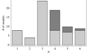
(b)

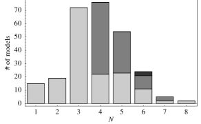
Figure 6.3: Hidden sector ‘rank’ distribution for (a) models with 3 nontrivial Wilson lines only, and (b) the combined set of models with 2 and 3 Wilson lines. $\mathrm{SU}(N)$/$\mathrm{SO}(2N)$/$\mathrm{E}_{N}$ are given by light/dark/darker bins.

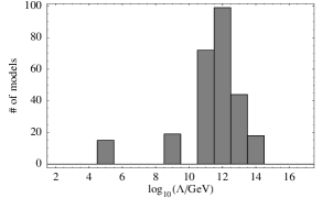
Figure 6.4: Number of mssm candidates with 2 and 3 Wilson lines vs. the scale of gaugino condensation.

Combining all models with two and three Wilson lines, we get the distribution peaking at $N=4$ displayed in fig. 6.3(b). The corresponding gaugino condensation scales are plotted in fig. 6.4. Notice that fig. 6.4 is almost identical to fig. 5.4, obtained in the case with two Wilson lines. It is remarkable that, just as in the case with two Wilson lines, requiring the exact mssm spectrum in the observable sector constrains the hidden sector such that gaugino condensation at an intermediate scale is automatically preferred. This provides a top-down motivation for TeV scales in particle physics.

6.3 Other $\boldsymbol{\mathbbm{Z}_{N}}$ Orbifolds

$\mathbbm{Z}_{6}$-II orbifolds yield a rich set of mssm candidates. An interesting question is whether this property is particular to this kind of orbifolds. The fact that $\mathbbm{Z}_{3}$ is a subset of $\mathbbm{Z}_{6}$-II and, therefore, there is a complex plane with three equivalent fixed points could be one advantage of $\mathbbm{Z}_{6}$ against $\mathbbm{Z}_{4}$ orbifolds. However, we have seen that mssm candidates have rather a structure with only two equivalent matter generations. Hence, one might argue that $\mathbbm{Z}_{4}$ could also produce good mssm candidates.

In this section, we search for realistic models in the context of $\mathbbm{Z}_{3}$, $\mathbbm{Z}_{4}$, $\mathbbm{Z}_{6}$-I and $\mathbbm{Z}_{7}$ orbifold compactifications. We are interested in torsionless models with the properties ➀–➅, that is, models where the chiral matter matter reproduces the exact spectrum of the mssm and the exotic particles are vectorlike. We do not verify the explicit decoupling of the exotics.

criterion	$\mathbbm{Z}_{3}$	$\mathbbm{Z}_{4}$	$\mathbbm{Z}_{6}$-I	$\mathbbm{Z}_{7}$
maximal # of Wilson lines	$3$	$4$	$1$	$1$
➁ ineq. models	$\sim 3,500$	$\sim 261,000$	$\sim 4,600$	$\sim 630,000$
➂ SU(3)$\times$SU(2) gauge group	$964$	$46,816$	$1,193$	$344,255$
➃ 3 net $(\boldsymbol{3},\boldsymbol{2})$	$228$	$683$	$217$	$16,536$
➄ nonanomalous $\mathrm{U}(1)_{Y}\subset\mathrm{SU}(5)$	$99$	$508$	$123$	$4,046$
➅ spectrum $=$ 3 generations $+$ vectorlike	$0$	$0$	$30$	$1$

Table 6.4: Statistics of $\mathbbm{Z}_{N}$ orbifolds with factorizable lattices and maximal number of Wilson lines.

Our results are presented in table 6.4. In $\mathbbm{Z}_{3}$ and $\mathbbm{Z}_{4}$, there are several models with three generations of quarks and leptons and nonanomalous hypercharge. However, their matter content includes some exotics that are not vectorlike.

In contrast, there are $\mathbbm{Z}_{6}$-I and $\mathbbm{Z}_{7}$ orbifold models that fulfill all our requirements. It is remarkable that in $\mathbbm{Z}_{6}$-I about $0.7\%$ of the total of models have realistic properties. We observe that these models have one family located at a fixed point (with or without local gut). The other two families arise from different twisted and untwisted sectors. In fact, it has been suggested that this picture may be phenomenologically favored [44]. In this sense, $\mathbbm{Z}_{6}$-I viable models are similar to $\mathbbm{Z}_{6}$-II models with three Wilson lines. We find only one $\mathbbm{Z}_{7}$ orbifold model that passes our criteria.

This study tells us that, despite the fact that $\mathbbm{Z}_{6}$-II orbifolds with local guts are indeed very appealing, other regions of the orbifold landscape could also render interesting vacua. A complete analysis of the models found here and of other successful geometries, such as $\mathbbm{Z}_{12}$ [152], is beyond the scope of this thesis and will be done elsewhere.

6.4 A Word on $\boldsymbol{\mathrm{SO}(32)}$ Orbifolds

There are good reasons to think that $\mathrm{SO}(32)$ orbifolds are less promising than compactifications of the E${}_{8}\times$E${}_{8}$ heterotic string. First, spinor representations appear only at the orbifold fixed points (see appendix B for a complete discussion). Noticing that matter generations can be embedded in spinorial representations of $\mathrm{SO}(10)$ guts indicates that it is less likely to get models with mssm matter. Secondly, there appear larger gauge groups, such as $\mathrm{SU}(15)$ which are more difficult to get broken to $\mathcal{G}_{SM}$. Finally, the Wilson lines in $\mathrm{SO}(32)$ orbifolds are more constrained by modular invariance and the embedding conditions. This is due to the fact that the length of spinorial Wilson lines in $\mathrm{SO}(32)$ is larger than in E${}_{8}\times$E${}_{8}$.

However, these claims do not mean that the SM cannot appear from $\mathrm{SO}(32)$ heterotic orbifolds. Therefore, it is unexplainable that there has been almost no effort in trying to get realistic $\mathrm{SO}(32)$ compactifications. To amend this, we have performed a search of mssm candidates in $\mathbbm{Z}_{3}$, $\mathbbm{Z}_{4}$ and $\mathbbm{Z}_{6}$-II orbifolds. In $\mathbbm{Z}_{3}$ and $\mathbbm{Z}_{4}$ orbifold models, the situation is quite similar to that of E${}_{8}\times$E${}_{8}$ orbifolds. At step (5) we find some models (comparatively, less models than in E${}_{8}\times$E${}_{8}$), but none of them is retained after demanding vectorlikeness of the exotics, at step (6).

In $\mathbbm{Z}_{6}$-II orbifolds the situation is different. We have studied models with arbitrary shift vector and up to two Wilson lines. There are about $380,000$ inequivalent models. Among them, only $2,276$ models have the sm gauge group, including nonanomalous hypercharge and three generations of quarks and leptons. The exotic particles can be decoupled from the low-energy spectrum in $87$ of these models.

It is noteworthy to compare our findings in $\mathrm{SO}(32)$ and E${}_{8}\times$E${}_{8}$. First of all, in E${}_{8}\times$E${}_{8}$ we have found a total of $352$ models with up to two Wilson lines at step (6), that is, about a factor $4$ more models than in $\mathrm{SO}(32)$. This is related to the difficulty of getting spinors in $\mathrm{SO}(32)$ orbifolds. On the other hand, looking at the low energy spectrum, the features of the models in both scenarios are very similar. In addition, we find that a good fraction (about $70\%$) of the $\mathrm{SO}(32)$ models exhibit local guts too. From these results, it seems reasonable to argue that there is no valid explanation to disregard semirealistic constructions appearing from the $\mathrm{SO}(32)$ heterotic string. In the following section we present some properties of one promising $\mathrm{SO}(32)$ orbifold. A complete discussion of these models and their phenomenological potential will be done elsewhere.

6.4.1 Phenomenology of SO(32) Orbifolds

In order to illustrate the qualities of potentially realistic $\mathrm{SO}(32)$ orbifolds, let us consider a $\mathbbm{Z}_{6}-$II orbifold model parametrized by the following gauge embedding:

$$V = \tfrac{1}{6}\left(3^{2},\,-1^{3},\,-2^{2},\,-3^{9}\right)\,,$$

$$A_{3} = \tfrac{1}{3}\left(0,\,3,\,1^{2},\,-1,\,0,\,-2,\,0^{2},\,-3,\,1^{2},\,-1,\,0,\,1^{2}\right)\,,$$ (6.4)

$$A_{5} = \tfrac{1}{2}\left(1^{2},\,-1,\,0,\,1,\,-1,\,1,\,-1^{2},\,0^{3},\,1^{4}\right)\,.$$

The unbroken gauge group in four dimensions is $\mathcal{G}_{4D}=\mathcal{G}_{SM}\times$ SO(10) $\times$ U(1)${}^{7}$, where the hypercharge generator takes the gut–like form

$$t_{Y}~{}=~{}\left(0^{10},\,\tfrac{1}{2}^{2},\,\tfrac{1}{3},\,0,\,-\tfrac{1}{3}^{2}\right)\,.$$ (6.5)

The matter spectrum of this model is provided in table 6.5. It comprises three mssm matter families plus additional vectorlike exotics, which decouple from the low energy theory at order 8 in singlets $\widetilde{s}=\{s^{0}_{i},\chi_{i}\}$, once these states acquire VEVs. In the generic vacuum, the relevant mass matrices are given by

$$\mathcal{M}_{d\bar{d}} \!\!\!\!\!=\! \!\!\!\!\!\left(\begin{array}[]{cccccc}\widetilde{s}&\widetilde{s}^{3}&\widetilde{s}&\widetilde{s}&\widetilde{s}&\widetilde{s}\\ \widetilde{s}^{5}&\widetilde{s}&\widetilde{s}^{3}&\widetilde{s}^{3}&\widetilde{s}^{3}&\widetilde{s}^{3}\\ \widetilde{s}^{5}&\widetilde{s}&\widetilde{s}^{3}&\widetilde{s}^{3}&\widetilde{s}^{3}&\widetilde{s}^{3}\end{array}\right)\;,$$ (6.6ae)

$$\mathcal{M}_{w\bar{w}}\!\! \!\!=\!\! \!\!\!\!\left(\begin{array}[]{cccc}\widetilde{s}^{2}&\widetilde{s}&\widetilde{s}^{2}&\widetilde{s}^{4}\\ \widetilde{s}^{5}&\widetilde{s}^{5}&\widetilde{s}^{5}&\widetilde{s}^{5}\\ \widetilde{s}^{2}&\widetilde{s}^{4}&\widetilde{s}^{2}&\widetilde{s}\\ \widetilde{s}^{5}&\widetilde{s}^{5}&\widetilde{s}^{5}&\widetilde{s}^{5}\\ \end{array}\right)\;.$$ (6.6aj)

Due to their size, we omit here $\mathcal{M}_{s^{+}s^{-}}$ and $\mathcal{M}_{mm}$.

Furthermore, the additional gauge bosons of U(1)${}^{7}$ also get massive, leaving only $\mathcal{G}_{\rm hidden}=$ SO(10) unbroken that serves to achieve a proper scale of susy breaking through gaugino condensation. Among the nonvanishing couplings, we find one unsuppressed trilinear coupling $q\bar{\phi}\bar{u}$, which indicates that the top quark acquires a mass hierarchically larger than the mass of the other quarks.

#	Representation	Label		#	Representation	Label
4	$\left(\boldsymbol{3},\boldsymbol{2};\boldsymbol{1}\right)_{(1/6,1/3)}$	$q_{i}$		1	$\left(\overline{\boldsymbol{3}},\boldsymbol{2};\boldsymbol{1}\right)_{(-1/6,-1/3)}$	$\bar{q}_{i}$
4	$\left(\overline{\boldsymbol{3}},\boldsymbol{1};\boldsymbol{1}\right)_{(-2/3,-1/3)}$	$\bar{u}_{i}$		1	$\left(\boldsymbol{3},\boldsymbol{1};\boldsymbol{1}\right)_{(2/3,1/3)}$	$u_{i}$
4	$\left(\boldsymbol{1},\boldsymbol{1};\boldsymbol{1}\right)_{(1,1)}$	$\bar{e}_{i}$		1	$\left(\boldsymbol{1},\boldsymbol{1};\boldsymbol{1}\right)_{(-1,-1)}$	$e_{i}$
6	$\left(\overline{\boldsymbol{3}},\boldsymbol{1};\boldsymbol{1}\right)_{(1/3,-1/3)}$	$\bar{d}_{i}$		3	$\left(\boldsymbol{3},\boldsymbol{1};\boldsymbol{1}\right)_{(-1/3,1/3)}$	$d_{i}$
8	$\left(\boldsymbol{1},\boldsymbol{2};\boldsymbol{1}\right)_{(-1/2,-1)}$	$\ell_{i}$		5	$\left(\boldsymbol{1},\boldsymbol{2};\boldsymbol{1}\right)_{(1/2,1)}$	$\bar{\ell}_{i}$
5	$\left(\boldsymbol{1},\boldsymbol{2};\boldsymbol{1}\right)_{(-1/2,0)}$	$\phi_{i}$		5	$\left(\boldsymbol{1},\boldsymbol{2};\boldsymbol{1}\right)_{(1/2,0)}$	$\bar{\phi}_{i}$
8	$\left(\overline{\boldsymbol{3}},\boldsymbol{1};\boldsymbol{1}\right)_{(1/3,2/3)}$	$\bar{\delta}_{i}$		8	$\left(\boldsymbol{3},\boldsymbol{1};\boldsymbol{1}\right)_{(-1/3,-2/3)}$	$\delta_{i}$
20	$\left(\boldsymbol{1},\boldsymbol{1};\boldsymbol{1}\right)_{(1/2,*)}$	$s^{+}_{i}$		20	$\left(\boldsymbol{1},\boldsymbol{1};\boldsymbol{1}\right)_{(-1/2,*)}$	$s^{-}_{i}$
17	$\left(\boldsymbol{1},\boldsymbol{1};\boldsymbol{1}\right)_{(0,1)}$	$\bar{n}_{i}$		14	$\left(\boldsymbol{1},\boldsymbol{1};\boldsymbol{1}\right)_{(0,-1)}$	$n_{i}$
4	$\left(\boldsymbol{3},\boldsymbol{1};\boldsymbol{1}\right)_{(-1/6,*)}$	$w_{i}$		4	$\left(\overline{\boldsymbol{3}},\boldsymbol{1};\boldsymbol{1}\right)_{(1/6,*)}$	$\bar{w}_{i}$
1	$\left(\boldsymbol{1},\boldsymbol{1};\boldsymbol{10}\right)_{(0,0)}$	$h_{i}$		16	$\left(\boldsymbol{1},\boldsymbol{2};\boldsymbol{1}\right)_{(0,*)}$	$m_{i}$
6	$\left(\boldsymbol{1},\boldsymbol{1};\boldsymbol{1}\right)_{(0,\pm 2)}$	$\chi_{i}$		68	$\left(\boldsymbol{1},\boldsymbol{1};\boldsymbol{1}\right)_{(0,0)}$	$s^{0}_{i}$

Table 6.5: Spectrum. The quantum numbers under SU(3)${}_{C}\times$SU(2)${}_{L}\times$ SO(10) are shown in boldface; hypercharge and $B\!-\!L$ charge appear as subscripts. Note that the states $s_{i}^{\pm}$, $w_{i}$, $\bar{w}_{i}$ and $m_{i}$ have different $B-L$ charges for different $i$, which we do not explicitly list.

It is possible to identify the nonanomalous $B\!-\!L$ generator

$$t_{B\!-\!L}~{}=~{}\left(0^{9},2,\,-1^{2},\,\tfrac{1}{3},\,0,\,-\tfrac{1}{3}^{2}\right)$$ (6.7)

under which some particles $\chi_{i}$ have $B\!-\!L$ charges $\pm 2$. The existence of U(1)${}_{B\!-\!L}$ has three direct consequences: first, it allows us to distinguish between lepton doublets $\ell_{i}$ and Higgs fields $\phi_{i}$, and between $\mathcal{G}_{\rm SM}\times$ U(1)${}_{B\!-\!L}$ singlets $\{s^{0}_{i},\,h_{i}\}$ and right–handed neutrinos $\bar{n}_{i}$; second, dimension four proton decay operators are forbidden; and third, couplings such as $(s^{0})^{n}\chi_{i}\bar{n}_{j}\bar{n}_{k}$ grant Majorana masses for the right–handed neutrinos. Note that, as before, if the fields $\chi_{i}$ attain VEVs, U(1)${}_{B\!-\!L}$ is spontaneously broken by two units to a $\mathbbm{Z}_{2}$ matter parity. Consequently, not only $\bar{n}_{i}$ but also $n_{i}$ shall correspond to right–handed neutrinos, giving a total of 31 right–handed neutrinos. We have verified that the corresponding mass matrix has full rank, implying that the masses of theses states is just below the string scale. As discussed in detail in section 5.5, the larger the number $N$ of heavy singlets the smaller the effective mass induced for the seesaw mechanism, $M_{*}\propto N^{-x}$ with $0<x<2$. The largest left–handed neutrino mass is then given by

$$M_{\mathrm{eff}}~{}\sim~{}v_{u}^{2}/M_{*}\,,$$ (6.8)

where $v_{u}$ corresponds to the VEV of the physical up–Higgs.

Another interesting property of this model is provided by the hidden sector, $\mathcal{G}_{\rm hidden}=$ SO(10). As discussed in section 5.3, assuming dilaton stabilization and gaugino condensation, the gravitino mass is fixed by the beta function of the hidden local interactions. In the current model, from eq. (5.72) follows that $b^{\mathrm{SO}(10)}_{0}=23$ and, consequently,

$$m_{3/2}\approx\frac{\Lambda^{3}}{M_{\mathrm{Pl}}^{2}}\approx\frac{2.1\times 10^{13}\ {\rm GeV}}{M_{\mathrm{Pl}}^{2}}\approx 9\ {\rm TeV}\,,$$ (6.9)

which fits well the usual expectations.

6.4.2 SO(32) Orbifolds, String Dualities and Prospects

We have seen in the previous section, that many appealing properties observed before in E${}_{8}\times$E${}_{8}$ models reappear in $\mathrm{SO}(32)$ constructions. Let us first contrast here the features of the $\mathrm{SO}(32)$ model with those of the Orbifold-mssm introduced in section 5.1. By mere comparison of the number of massless states, one sees that they are different. From the point of view of the spectrum, a phenomenological disadvantage of the $\mathrm{SO}(32)$ model is the number of quark doublets $q_{i}$. In the Orbifold-mssm there are only three of these states, two of them localized at the fixed points. This allows us to associate a geometrical picture to the origin of the hierarchy between the heavy family (in particular, the heavy top) and the two lighter generations. This picture is enhanced by the fact that a contribution to the physical Higgs $\bar{\phi}$ appears in the untwisted sector, yielding naturally an unsuppressed mass term for the top quark. In the $\mathrm{SO}(32)$ model, this intuition is lost and the existence of a large mass for the top quark seems rather accidental.

In fact, one can compare all models with phenomenologically attractive properties in both heterotic cases. We find that, at massless level, the spectra are all inequivalent. This can be easily explained by the fact that some (sm) matter generations in the E${}_{8}\times$E${}_{8}$ stem directly from the gauge fields whereas in $\mathrm{SO}(32)$ this cannot occur as spinors are not embedded into the adjoint representation $\boldsymbol{496}$.

However, it is well known that the heterotic E${}_{8}\times$E${}_{8}$ and $\mathrm{SO}(32)$ theories are related by T-duality. Therefore, one would expect that a large-volume E${}_{8}\times$E${}_{8}$ orbifold compactification can yield an identical theory in $\mathrm{SO}(32)$ when compactifying in an orbifold with small volume. Yet at the stage of the current analysis, due to the features mentioned before, it seems clear that the promising models we find are truly different. It might be interesting to verify whether the $\mathbbm{Z}_{6}$–II promising models in one heterotic theory can be found in a different $\mathbbm{Z}_{N}$ or $\mathbbm{Z}_{N}\times\mathbbm{Z}_{M}$ compactification. We note that it is also possible that an orbifold model in one theory could be only identified with a model from the dual theory just after blowing up the orbifold singularities [153]. Therefore, it is natural to wonder whether the dual model can be found among orbifold compactifications at all, or one should rather investigate other constructions such as fermionic models or Calabi-Yau compactifications.

Another interesting relation is provided by S-duality. It connects the weakly coupled $\mathrm{SO}(32)$ heterotic string with the strongly coupled type I theory and vice versa [154]. Some effort in the construction of semirealistic four-dimensional compactifications has been done [155, 156] via a $\mathbbm{Z}_{3}$ orbifold. However, as far as we know, none of these constructions groups all the properties of the heterotic orbifold models discussed in this work. Therefore, establishing the connection between heterotic $\mathrm{SO}(32)$ orbifolds and type I compactifications requires first a bigger effort in the context of type I.

Chapter 7 Conclusions and Outlook

In this thesis we have discussed orbifold compactifications of the heterotic string. We have emphasized their relation to low–energy phenomenology and, therefore, its viability as a unified theory of all observed forces. In particular, we have focused on the phenomenology of abelian orbifold compactifications of the $\mathrm{E}_{8}$$\times$$\mathrm{E}_{8}$ heterotic string theory.

We have briefly described the heterotic string and provided some recipes for the computation of the direct properties of symmetric abelian orbifold models, such as their fixed points and their matter spectra. We have also discussed the role that some additional degrees of freedom denominated discrete torsion play in theses constructions. In concrete, we have seen that discrete torsion alters the chiral-matter content of the orbifold. We have shown that, contrary to previous statements, $\mathbbm{Z}_{N}$ orbifolds with Wilson lines as well as $\mathbbm{Z}_{N}\times\mathbbm{Z}_{M}$ orbifold models admit discrete torsion. Further, we have found out that the assignments of discrete torsion can be traded for translations of the gauge embedding parameters (shifts and Wilson lines) in the gauge lattice $\Lambda$.

We have explained and extended some conventional methods employed to classify orbifold models, paying special attention to the construction of ansätze that allow us to obtain systematically all inequivalent input parameters of orbifold compactifications. The proposed classification methods are very flexible and can be adapted to both ($\mathrm{E}_{8}$$\times$$\mathrm{E}_{8}$ and $\mathrm{SO}(32)$) heterotic string theories. Our methods have already been tested in all $\mathbbm{Z}_{N}$ and $\mathbbm{Z}_{N}\times\mathbbm{Z}_{M}$ orbifolds. We have made an exhaustive classification of $\mathbbm{Z}_{N}$ orbifolds without background fields and also a complete classification of $\mathbbm{Z}_{3}$$\times$$\mathbbm{Z}_{3}$ orbifold models, including discrete torsion. Whenever possible, we have compared our results to those of the literature.

To address the question of whether there are realistic orbifold compactifications, we have analyzed the heterotic $\mathrm{E}_{8}$$\times$$\mathrm{E}_{8}$ string compactified on a $\mathbbm{Z}_{6}$-II orbifold, allowing for up to two discrete Wilson lines. Using a search strategy based on the concept of local guts, we have obtained about $3\times 10^{4}$ inequivalent models. Out of them, 223 models exhibit the mssm gauge group structure, three light families and vectorlike exotics. We show that all the vectorlike exotics can decouple without breaking supersymmetry for 190 of these models. This means that almost 1 % out of $3\times 10^{4}$ models have the gauge group and the chiral matter content of the mssm. This result shows that orbifold compactifications of the heterotic string correspond to a particularly fertile region in the landscape and that the probability of getting something close to the mssm is significantly higher than that in other constructions. It would be interesting to extend these results to other regions of the landscape where some promising models also exist.

Furthermore, we have found that requiring realistic features in the set of mssm candidates is correlated with the supersymmetry breaking scale such that, in the context of gaugino condensation, intermediate scale ($\sim 1$ TeV) of susy breaking is favored. This occurs because most of the models with realistic features have a hidden sector with $\mathrm{SU}(4)$ or $\mathrm{SO}(8)$ nonabelian symmetry.

In order to get closer to the mssm, we defined a successful strategy for obtaining models with an exact $R$-parity based on spontaneous breaking of a gauge $\mathrm{U}(1)_{B\!-\!L}$ symmetry. We find 87 models which have a renormalizable top Yukawa coupling. Out of these, we identify 15 models with an exact $R$-parity, no light exotics or $\mathrm{U}(1)$ gauge bosons and an order one top quark Yukawa coupling. We would like to remark that the number 15 is a lower bound, mainly since our search is based on a specific strategy related to $B\!-\!L$ symmetry. Additionally, many of our constraints, such as demanding a renormalizable coupling for the top quark are just artifacts invoked in order to simplify our analysis. Therefore, an interesting question would be to obtain similar results in cases where: a) no trilinear coupling for the top quark is demanded, b) no vectorlikeness of the sm matter generations with respect to $B\!-\!L$ is imposed, c) also models with anomalous $B\!-\!L$ are admitted, and d) $R$-parity results directly from the so-called R-charge conservation (string) selection rule.

On the other hand, we notice that dimension five baryon and lepton number violating operators, like $q\,q\,q\,\ell$, appear in orbifold models quite regularly even if $B\!-\!L$ is imposed. They are either generated in the superpotential to some order in sm singlets, or they may also be generated when integrating out heavy exotics. In some cases, only fine-tuning the vevs of some sm singlets can alleviate this problem. One is thus encouraged to investigate other possible solutions, such as the identification of some discrete symmetries.

Another aspect of phenomenology we have studied is the seesaw mechanism. Since there are no upper bounds on the amount of right–handed neutrinos that might appear, we find that in a scenario with $\mathcal{O}(100)$ right–handed neutrinos, the seesaw mechanism is realized from orbifold constructions. Moreover, (left–handed) neutrino masses are then enhanced (in comparison to the naïve estimate of the neutrino masses in guts) to more realistic values. We consider this setup to be plausible and perhaps even desirable, since some consequences of the existence of many right–handed neutrinos could shed some light in some open issues, such as leptogenesis [157, 158]. We might even consider the abundance of right–handed neutrinos to be a prediction of string theory.

We have also studied in detail one model that we have called orbifold-mssm. The propertiesof this model are generic in the sense that other mssm candidates possess very similar qualities: only the exact matter spectrum of the mssm (up to many sm singlet fields); admissible $B\!-\!L$ symmetry which is spontaneously broken to matter parity in a supersymmetric vacuum configuration; gaugino condensation scale leading to susy breaking at an intermediate scale; vanishing $\mu$–term; and proton decay through dimension five operators can be avoided by some fine-tuning. The top Yukawa coupling is order $\widetilde{s}^{2}$ due to Higgs doublet mixing in this model. Further, both the up and down quarks are massless at order six in sm singlets. However, the up quark becomes massive at order seven and the down quark gets a mass at order eight. These properties are very interesting, but we believe that the best model awaits still in some corner of the landscape.

Finally, we have extended our search of models with realistic features to $\mathbbm{Z}_{6}$-II orbifold models with three Wilson lines. Out of a total of $10^{7}$, we have found almost 300 inequivalent models with the mssm spectrum and gauge coupling unification. Most of these models originate from local guts. We also found that low energy supersymmetry breaking is also favored in these models. Further, we have explored $\mathbbm{Z}_{3}$, $\mathbbm{Z}_{4}$, $\mathbbm{Z}_{6}$-I and $\mathbbm{Z}_{7}$ orbifolds searching for promising models. We have found small sets of realistic models in $\mathbbm{Z}_{6}$-I and $\mathbbm{Z}_{7}$ orbifolds. This suggests that a broader scan could also help to understand how the mssm may be embedded in string theory.

There are some phenomenological issues that we have not addressed in this thesis. In particular, one issue concerns proton stability. The examples we studied are challenged by the presence of dimension five proton decay operators. Their suppression may require additional (discrete) symmetries or even a change in the geometry of the orbifold, as suggested in appendix C. There are also dimension six operators, generated by gut gauge boson exchange, which we have not discussed.

Further, we have not studied precision gauge coupling unification. Although hypercharge is normalized as in four-dimensional guts thus allowing gauge coupling unification in the first approximation, there are various corrections that can be important. First, a detailed analysis would require the calculation of string threshold corrections in the presence of discrete Wilson lines. However in specific cases these corrections are known to be small [159]. Second, there are corrections from the vectorlike exotic states. It is possible that precision gauge coupling unification may require anisotropic compactifications, leading to an effective orbifold gut. [160, 161, 41, 162]. These questions have been explored in ref. [163] and refs. [164, 165].

Another question that was not clarified in this thesis concerns moduli stabilization. We have seen that, e.g. in order to determine the scale of gaugino condensation, stabilizing the dilaton $S$ is crucial. The minimum of its potential affects strongly the scale of supersymmetry breakdown in the observable sector. However, the dilaton is not the sole modulus in the theory. Beside some geometrical moduli, many singlet fields (with neither vevs nor masses) appear in the matter spectrum of orbifolds. Their stabilization is also important for addressing cosmological issues, such as inflation and baryogenesis.

Appendix A Form of Shift Vectors and Wilson lines

Even though there is a straightforward prescription to obtain all $\mathbbm{Z}_{N}$ shift vectors (see section 3.1), it is necessary to implement a method which can be easily extended to $\mathbbm{Z}_{N}\times\mathbbm{Z}_{M}$ orbifolds and orbifolds with Wilson lines. An option is an ansatz that describes any shift or Wilson line. To start with, let us specify an ansatz for $\mathbbm{Z}_{N}$ shifts of $\mathrm{SO}(32)$ orbifolds. We will see in section A.2 that the resulting ansatz can be then trivially generalized.

A.1 $\boldsymbol{\mathbbm{Z}_{N}}$ Shift Vectors of $\boldsymbol{\mathrm{SO}(32)}$ Orbifolds

We will call vectorial shifts to those shift vectors of order $N$ ($NV\in\Lambda$) whose entries have a maximal denominator of $N$. Spinorial shifts will be those other which have a denominator of $2N$ and an odd numerator. As an example, consider the $\mathbbm{Z}_{4}$ shift vectors of table D.5. The first 12 of them are vectorial, whereas the last four are spinorial. It is convenient to describe separately these two cases and further distinguish between $\mathbbm{Z}_{N}$ shifts with $N$ even and $N$ odd.

To obtain the general form of a shift, we take for granted that two shift vectors are equivalent if they are related by lattice vectors or by Weyl reflections, i.e. by any permutation of the entries and pairwise sign flips.

a) Vectorial Shifts and $\boldsymbol{N}$ Even

Invariance under lattice translations implies that the entries $V_{i}$ of a shift of order $N$ are constrained by $-(N-1)/N\leq V_{i}\leq 1$. Therefore, we can start with the ansatz

$$V=\frac{1}{N}\big{(}-(N-1)^{n_{-(N-1)}},\,-(N-2)^{n_{-(N-2)}},\ldots,\,0^{n_{0}},1^{n_{1}},\ldots,N^{n_{N}}\big{)}$$ (A.1)

for a vectorial shift. As usual, the exponent $n_{i}$ of an entry $i$ counts how many times that entry is repeated; for instance, the entry $-(N-1)$ appears $n_{-1(N-1)}$ times. Therefore, the exponents $n_{i}$ are integers satisfying

$$\sum_{i}n_{i}=16\;.$$ (A.2)

Since pairwise sign-flips are allowed, we see that all negative entries can be made nonnegative as long as at least one $n_{-i}$ is even ($i=1,\ldots,N$). However, if there is an odd number of negative entries and $n_{0}=0$, one negative entry will remain. Combining both results, we get

$$V=\frac{1}{N}\big{(}(-j)^{\alpha},\,0^{n_{0}},1^{n_{1}},\ldots,j^{n_{j}-\alpha},\ldots,(N-1)^{n_{N-1}}\big{)}\,,\;\;\qquad 1\leq j\leq N-1$$ (A.3)

with $\alpha=0,1$. This ansatz contains still some redundancies. Lattice translations of the shifts amounts to adding $\pm 1$ to an even number of entries of $V$. One can thus apply $V_{i}\rightarrow V_{i}-1$ for an even number of entries fulfilling $V_{i}>\frac{N}{2}$ and then flip their signs. By this operation, a $\mathbbm{Z}_{N}$ vectorial shift can be finally expressed by

$$V=\frac{1}{N}\left((\pm j)^{\alpha},-(N-j)^{\beta},0^{n_{0}},1^{n_{1}},\ldots,(N-j)^{n_{(N-j)}-\alpha-\beta},\ldots,\left(\frac{N}{2}\right)^{n_{\frac{N}{2}}}\right)\,,$$ (A.4)

where $\alpha,\beta=0,1$ such that $\alpha+\beta=0,1$ and $j$ can take the values $\{\frac{N}{2}+1,\ldots,N-1\}$.

As a side remark, using the shift $V$ of eq. (A.4) and the $\mathrm{SO}(32)$ simple roots $\alpha_{i}$ provided in table D.7, one can compute $\alpha_{i}\cdot V$. Since those roots with $\alpha_{i}\cdot V\neq 0$ are projected out while the others form the Dynkin diagram of the unbroken gauge group $\mathcal{G}_{4D}$, one finds that the symmetry breakdown induced by a generic vectorial shift of $\mathrm{SO}(32)$ orbifolds is given by

$$\mathrm{SO}(32)\longrightarrow\mathrm{SO}(2n_{0})\times\mathrm{U}(n_{1})\times\ldots\times\mathrm{U}(n_{\left(\frac{N}{2}-1\right)})\times\mathrm{SO}(2n_{N/2})\,,$$ (A.5)

recalling that $\mathrm{U}(n)=\mathrm{SU}(n)\times\mathrm{U}(1)$.

b) Spinorial Shifts and $\boldsymbol{N}$ Even

An analogous analysis to that presented in the previous case leads to the conclusion that a generic spinorial shift can be written as

$$V=\frac{1}{2N}\left((\pm j)^{\alpha},-(2N-j)^{\beta},1^{n_{1}},3^{n_{3}},\ldots,(2N-j)^{n_{(2N-j)}-\alpha-\beta},\ldots,(N-1)^{n_{N-1}}\right)\,,$$ (A.6)

with $j\in\{N+1,N+3,\ldots,2N-1\}$. It is again not hard to confirm that a shift vector of this kind leads to the breaking

$$\mathrm{SO}(32)\longrightarrow\mathrm{U}(n_{1})\times\mathrm{U}(n_{3})\times\ldots\times\mathrm{U}(n_{N-3})\times\mathrm{U}(n_{N-1})\,.$$ (A.7)

c) $\boldsymbol{N}$ Odd

The general form of the shift vectors changes slightly. First, as explained in ref. [166], in this case it is enough to determine either the vectorial or the spinorial shifts, since one spinorial shift can always be transformed into a vectorial one by the action of Weyl reflections and lattice vectors. Choosing the vectorial form, we obtain the following shift vector of odd order:

$$V=\frac{1}{N}\left((\pm j)^{\alpha},-(N-j)^{\beta},0^{n_{0}},1^{n_{1}},\ldots,(N-j)^{n_{(N-j)}-\alpha-\beta},\ldots,\left(\frac{N-1}{2}\right)^{n_{\left(\frac{N-1}{2}\right)}}\right)\,,$$ (A.8)

where $j\in\{\frac{N+1}{2},\frac{N+3}{2},\ldots,N\}$. The resulting four dimensional gauge group is

$$\mathrm{SO}(32)\longrightarrow\mathrm{SO}(2n_{0})\times\mathrm{U}(n_{1})\times\ldots\times\mathrm{U}(n_{\left(\frac{N-3}{2}\right)})\times\mathrm{U}(n_{\left(\frac{N-1}{2}\right)})\,.$$ (A.9)

The shifts obtained by the ansätze given in eqs. (A.4)–(A.8) are further restrained by $NV\in\Lambda$ and the requirement that follows from invariance of the orbifold partition function:

$$N\left(V^{2}-v^{2}\right)=0\text{ mod }2$$ (A.10)

for a given twist vector $v$ of order $N$. Only those shifts satisfying these conditions are consistent with orbifold compactifications. The ansätze (A.4)–(A.8) constitute, as we will see in the next section, the basic constructing blocks of general $\mathbbm{Z}_{N}\times\mathbbm{Z}_{M}$ shifts and Wilson lines.

A.2 A General Ansatz

Now we are in position to propose an ansatz which covers all orbifolds, including Wilson lines. Consider a model with a given shift vector $V$. Independently of whether $V$ belongs to an $\mathrm{E}_{8}$$\times$$\mathrm{E}_{8}$ or an $\mathrm{SO}(32)$ orbifold, Weyl reflexions and lattice translations allow to make its entries as small as possible and to gather them in blocks $V_{\text{block i}}$, just as in the ansätze (A.4)–(A.8):

$$V=\frac{1}{N}\left(V_{\text{block 1}},\,V_{\text{block 2}},\,V_{\text{block 3}},\ldots\right)\,,$$ (A.11)

where each subvector $V_{\text{block i}}$ contains $m_{i}$ identical integer or half-integer entries, such that $\sum_{i}m_{i}=16$. Our task is then to find a universal second shift $V_{2}$ of order $M$, in the case of $\mathbbm{Z}_{N}\times\mathbbm{Z}_{M}$ orbifolds, or/and the general form of a Wilson line $A_{\alpha}$ of order $N_{\alpha}$, trying to avoid redundancies at maximum. From the block-structure of the shift vector, we can expect $V_{2}$ and $A_{\alpha}$ also to be splitted in blocks of length $m_{i}$ as

$$V_{2} = \left(V_{2,\text{block 1}},\,V_{2,\text{block 2}},\,V_{2,\text{block 3}},\ldots\right)\,,$$ (A.12a)

$$A_{\alpha} = \left(A_{\alpha,\text{block 1}},\,A_{\alpha,\text{block 2}},\,A_{\alpha,\text{block 3}},\ldots\right)\,.$$ (A.12b)

This would mean that each block $V_{2,\text{block i}}$ and $A_{\alpha,\text{block i}}$ is independent and can, therefore, be described separately. In other words, we have just to find an ansatz for a subvector $V_{2,\text{block i}}$ or $A_{\alpha,\text{block i}}$ of the corresponding order ($M$ or $N_{\alpha}$) and then to apply it consecutively over all blocks.

In the previous section, we have seen that the ansätze (A.4)–(A.8) describe the minimal form of a shift of order $N$. They can be used in order to build the blocks $V_{2,\text{block i}}$ and $A_{\alpha,\text{block i}}$, by replacing $N$ by $M$ or $N_{\alpha}$ and demanding that

$$\sum_{j}n_{j}=m_{i}$$ (A.13)

for each block. We have additionally to guarantee that the vectors obtained in this way lie on the lattice $\Lambda$, i.e. one has to impose $MV_{2},\,N_{\alpha}A_{\alpha}\in\Lambda$. This condition implies that, for even $N$, all blocks must be of the same type (either vectorial or spinorial). Clearly, admissible orbifold models are only those with shift(s) and Wilson lines fulfilling the modular invariance conditions provided in eq. (2.58).

Appendix B Spinors in SO(32) Orbifolds

Early works on orbifold compactifications considered the $\mathrm{SO}(32)$ heterotic string to be phenomenologically disfavored. One of the reasons being that the theory by itself does not include spinors in its massless spectrum. This situation was shown to be preserved in the simplest orbifold compactifications, leading to the somewhat naïve conclusion that, if spinors can be found from the $\mathrm{SO}(32)$ heterotic string at all, they must appear in a quite unnatural way.

Only recently, the interest in four-dimensional heterotic $\mathrm{SO}(32)$ orbifold constructions has been revived [167, 168]. In the case of $\mathbbm{Z}_{N}$ orbifolds, a complete classification of gauge embeddings in the absence of background fields has been achieved [166, 47]. Interestingly, that classification has shown that spinors of $\mathrm{SO}(2n)$ gauge groups appear rather frequently in the twisted sectors of $\mathrm{SO}(32)$ orbifolds. Spinors of $\mathrm{SO}(10)$, in particular, are found locally at fixed points of the first twisted sector of many orbifold models. Moreover, that classification reveals that the amount of available $\mathrm{SO}(32)$ orbifold models is comparable, at the same level, to that of its more famous brother: the $\mathrm{E}_{8}\times\mathrm{E}_{8}$ string. Thus, it is not adventurous rather to conclude that model building based on the heterotic $\mathrm{SO}(32)$ string theory might be as interesting as that based on the $\mathrm{E}_{8}\times\mathrm{E}_{8}$ theory.

On the other hand, the appearance of spinors on models derived from the $\mathrm{SO}(32)$ heterotic string might also be important for a possible understanding of the $\mathrm{SO}(32)$ heterotic type I duality in four spacetime dimensions. We know that spinors do not appear in the perturbative type I theory. Thus, the mentioned duality requires the implementation of nonperturbative effects.

B.1 $\boldsymbol{\mathrm{SO}(10)}$ Spinors and Shift Vectors

Let us investigate here the possibility of having the 16-dimensional spinor representation of SO(10) in $\mathbbm{Z}_{N}$ orbifolds of the $\mathrm{SO}(32)$ heterotic string theory. In the standard basis of the roots of $\mathrm{SO}(10)$, the highest weight of the $\boldsymbol{16}$–plet is given by the five-dimensional vector 

$$\boldsymbol{16}_{\text{HW}}=\left(\frac{1}{2}^{5}\right)\,.$$ (B.1)

To be included in the spectrum of an orbifold compactification, this vector must be part of a 16-dimensional solution $p_{\text{sh}}$ to the mass formula for massless states, eq. (2.84) or eq. (2.97). Therefore, $p_{\text{sh}}$ must be written as

$$p_{\text{sh}}~{}=~{}p+V_{g}~{}=~{}\left(\frac{1}{2}^{5},\,a_{1},\,\ldots,\,a_{11}\right)\,,$$ (B.2)

where $p\in\Lambda_{\text{Spin(32)}/\mathbbm{Z}_{2}}$, $V_{g}$ is the local shift of a constructing element $g$ and $a_{i}\in\mathbbm{R}$ are selected so that $p_{\text{sh}}$ fulfills $Np_{\text{sh}}\in\Lambda_{\text{Spin(32)}/\mathbbm{Z}_{2}}$ and the mass formula. There can be more than one combination of different $a_{i}$’s for which the resulting $p_{\text{sh}}$ satisfies all the conditions.

A first consequence of eq. (B.2) is that one cannot get $\boldsymbol{16}$–plets of $\mathrm{SO}(10)$ in the untwisted sector of any orbifold compactification. The reason is that the only $p_{\text{sh}}$ available for untwisted massless states correspond to the roots of $\mathrm{SO}(32)$, which are expressed by the 480 vectors $(\underline{\pm 1,\,\pm 1,\;0^{14}})$.

As a second consequence, one finds that it is not possible to get $\boldsymbol{16}$–plets of $\mathrm{SO}(10)$ in the $\mathbbm{Z}_{3}$ orbifold. This can be understood as follows. Since in $\mathbbm{Z}_{3}$ orbifolds $3p_{\text{sh}}$ must lie on the lattice $\Lambda_{\text{Spin(32)}/\mathbbm{Z}_{2}}$ and the first five entries of $3p_{\text{sh}}$ are half-integer, all $a_{i}$’s must also be half-integer, $3a_{i}\in\mathbb{Z}+1/2$. Assuming in the best of the cases that $3a_{i}=1/2$, it follows that $p_{\text{sh}}^{2}\geq 14/9$. However, masslessness of the states in $\mathbbm{Z}_{3}$ orbifolds constrains $p_{\text{sh}}$ to have at most squared length $4/3$.

It is possible to find the form of the local shift vectors producing $\mathrm{SO}(10)$ spinors. From eq. (B.2), for all $\mathbbm{Z}_{N}$ orbifolds with $N>3$ the local shift(s) giving rise to the $\boldsymbol{16}$ representation of $\mathrm{SO}(10)$ can be written as

$$V_{g}~{}=~{}p_{\text{sh}}-p\,$$ (B.3)

with $p_{\text{sh}}$ given as in eq. (B.2).

Hence, we can determine the shift vector $V$ of an orbifold model containing $\mathrm{SO}(10)$ spinors in the first twisted sector, relevant for phenomenology, as we have discussed in section 4.1. In absence of Wilson lines, the local shift vector $V_{g}$ at any fixed point of the first twisted sector coincides with $V$, therefore

$$V~{}=~{}p_{\text{sh}}-p\stackrel{{\scriptstyle p=0}}{{\longrightarrow}}p_{\text{sh}},$$ (B.4)

where we have chosen $p=0$ because two shifts are equivalent if they differ by an arbitrary lattice vector. This shift vector is automatically modular invariant. For each allowed $p_{\text{sh}}$ from eq. (B.2), one can verify that the shift vector $V$ obtained through eq. (B.4) leads to a four-dimensional $\mathrm{SO}(10)$ gauge group by applying the patterns provided in appendix A.1.

As an example, we consider the $\mathbbm{Z}_{4}$ orbifold without Wilson lines. The only possible shift vector consistent with $4V\in\Lambda_{\text{Spin(32)}/\mathbbm{Z}_{2}}$, the masslessness condition eq. (2.97) and eq. (B.4) is

$$V~{}=~{}p_{\text{sh}}~{}=~{}\left(\frac{1}{2}^{5},\,\frac{1}{4}^{2},\,0^{9}\right)\,,$$ (B.5)

which is one of the admissible shift vectors for the $\mathbbm{Z}_{4}$ orbifold, listed in table D.5.

Appendix C $\boldsymbol{\mathbbm{Z}_{6}}$-II on Nonfactorizable Lattices

$\mathbbm{Z}_{6}$-II orbifold compactifications on the lattice $\mathrm{G}_{2}\times\mathrm{SU}(3)\times\mathrm{SO}(4)$ have proven to lead to realistic models. The question here is how the properties of such models are influenced by the use of one of the other allowed lattices of $\mathbbm{Z}_{6}$-II. In the best of the cases, the possible changes shall be of relevance when dealing with unsolved phenomenological issues such as proton decay.

C.1 Lattices and Spectrum

The allowed lattices of $\mathbbm{Z}_{6}$-II orbifolds are presented in table C.1. Note that, with exception of the lattice (A), $\mathrm{G}_{2}\times\mathrm{SU}(3)\times\mathrm{SO}(4)$, all lattices are nonfactorizable. These lattices are independent in the sense that they cannot be deformed continuously into one another. Therefore, one knows that orbifolds on those lattices will have certainly distinct properties.

The choice of the lattice of the compact space will affect some other properties. Firstly, one finds that the number of fixed points of the orbifold varies according to

$$\begin{array}[]{clccc}&\text{\bf Lattice}&\boldsymbol{T_{1}}&\boldsymbol{T_{2}}&\boldsymbol{T_{3}}\\ (A)&\mathrm{G}_{2}\times\mathrm{SU}(3)\times\mathrm{SO}(4)&12&6&8\\ (B)&\mathrm{SU}(3)\times\mathrm{SO}(8)&12&3&8\\ (C)&\mathrm{SU}(3)\times\mathrm{SO}(7)\times\mathrm{SU}(2)&12&3&8\\ (D)&\mathrm{SU}(6)\times\mathrm{SU}(2)&12&3&4\end{array}$$

where, as usual, $T_{i}$ denotes the $i^{\mathrm{th}}$ twisted sector. Secondly, the number and order of the allowed Wilson lines changes. In the factorizable lattice (A), we have seen that there are two order 2 Wilson lines corresponding to the $\mathrm{SO}(4)$ torus, and one independent order 3 Wilson line in the $\mathrm{SU}(3)$ torus. This contrasts e.g. to the lattice $\mathrm{SU}(6)\times\mathrm{SU}(2)$ in which only two Wilson lines are allowed: an order 2 Wilson line in the $\mathrm{SU}(2)$ torus and an order 6 Wilson line in the $\mathrm{SU}(6)$ torus. The number and order of the Wilson lines in all lattices are shown in table C.1.

These two features have crucial effects on the matter spectrum of orbifold models. Evidently, the number of states of orbifolds on nonfactorizable lattices will be reduced compared to the number of states on the usual lattice (A). What is somehow more interesting is that the missing states in nonfactorizable orbifolds form vectorlike pairs.

Consider, for instance, the spectrum of the orbifold-mssm  listed in table C.2. We see that the number of exotics is reduced by compactifying on nonfactorizable lattices. All nonfactorizable lattices (B,C,D) yield in the observable sector only three mssm generations plus two pairs of Higgses. That means that unwanted quark triplets and two Higgs pairs have disappeared. Notice that we lose simultaneously some needed particles, such as some sm singlets $s^{0},\,h$, used to decouple exotics, and some right-handed neutrinos $n,\,\bar{n},\,\eta,\,\bar{\eta}$. This is not a problem as long as the remaining exotics can still be decoupled.

	6D Lattice $\Gamma$	Twist $v$	Conditions on Wilson lines
(A)	$\mathrm{G}_{2}\times\mathrm{SU}(3)\times\mathrm{SO}(4)$	$\frac{1}{6}(0,\,1,\,2,\,-3)$	$3A_{3}\approx 2A_{5}\approx 2A_{6}\approx 0;\;A_{1}\approx A_{2}\approx 0,\,A_{3}\approx A_{4}$
(B)	$\mathrm{SU}(3)\times\mathrm{SO}(8)$	$\frac{1}{6}(0,\,2,\,1,\,-3)$	$3A_{1}\approx 2A_{5}\approx 0;\;A_{1}\approx A_{2},\,A_{3}\approx A_{4}\approx 0,\,A_{5}\approx A_{6}$
(C)	$\mathrm{SU}(3)\times\mathrm{SO}(7)\times\mathrm{SU}(2)$	$\frac{1}{6}(0,\,2,\,1,\,-3)$	$3A_{1}\approx 2A_{5}\approx 2A_{6}\approx 0;\;A_{1}\approx A_{2},\,A_{3}\approx A_{4}\approx 0$
(D)	$\mathrm{SU}(6)\times\mathrm{SU}(2)$	$\frac{1}{6}(0,\,2,\,1,\,-3)$	$6A_{1}\approx 2A_{6}\approx 0;\;A_{1}\approx A_{2}\approx A_{3}\approx A_{4}\approx A_{5}$

Table C.1: Allowed lattices for $\mathbbm{Z}_{6}$-II orbifolds and constraints on the Wilson lines. With exception of (A), all lattices are nonfactorizable.

This situation is similar to what is observed between brother models of $\mathbbm{Z}_{2}\times\mathbbm{Z}_{2}$ orbifolds. In that case, nonvanishing discrete torsion on orbifolds with a given torus lattice projects out some of the states living at particular fixed points, reducing thereby the effective number of fixed points. Hence, the massless spectra of models with discrete torsion on a given lattice turn out to be identical to the spectra of models without discrete torsion on a different lattice [48]. A natural question is then whether discrete torsion also relates the spectra of $\mathbbm{Z}_{6}$-II orbifolds compactified on different lattices. Unfortunately, a close inspection of the parameters of discrete torsion in $\mathbbm{Z}_{6}$-II orbifolds convinces us that discrete torsion (as introduced in ref. [48]) does not have any effect on the spectrum of the models. An interesting question is whether discrete torsion does not exhaust all the available degrees of freedom that alter orbifold models.

C.1.1 A Comment on the String Selection Rules

Compactifying on nonfactorizable lattices affects more than the spectrum. The computation of Yukawa couplings in factorizable orbifold models is based on certain selection rules stated in a form that appears to be related with the factorizability of the lattice. Particularly, conservation of $R$-charge in $\mathbbm{Z}_{6}$-II factorizable orbifolds is expressed as

$$\sum_{i}R^{1}_{i}=-1\mod 6\,,\;\;\;\sum_{i}R^{2}_{i}=-1\mod 3\,,\;\;\;\sum_{i}R^{3}_{i}=-1\mod 2\,,$$ (C.1)

where the sum runs over the states of a given coupling. $R^{a}_{i}$ corresponds to the R-charge of the $i^{\mathrm{th}}$ particle of the coupling on the $a^{\mathrm{th}}$ complex plane of the compact space.

In the literature [121, 169], it is usually stated that R-charge conservation, eq. (C.1), follows from the symmetries of the three complex planes of a factorizable orbifold. In the case of factorizable $\mathbbm{Z}_{6}$-II orbifolds, it is clear that the three independent (discrete) rotations generated by the Cartan generators $H^{a}$ of the underlying $\mathrm{SO}(6)$ ($\simeq\mathrm{SU}(4)$) Lorentz symmetry leave the compactification lattice (A) invariant. Therefore, the original $\mathrm{SO}(6)$ Poincaré symmetry of the compact space is broken to $\mathbbm{Z}_{6}\times\mathbbm{Z}_{3}\times\mathbbm{Z}_{2}$ in the factorizable orbifold.

We might assume that this also holds for compactifications on other lattices and then we could apply the same R-charge conservation given in eq. (C.1). However, in this case, the relation between R-charge conservation and complex-plane rotation invariance is violated in nonfactorizable lattices. For example, consider the lattice $\mathrm{SU}(6)$$\times$$\mathrm{SU}(2)$. One can show that the only element of $\mathrm{SO}(6)$ containing only Cartan generators that leaves the lattice invariant is

$$\boldsymbol{R^{t}}\equiv e^{2\pi\mathrm{i}\frac{1}{6}(2H_{1}+H_{2}-3H_{3})}$$ (C.2)

and powers of it. We can then conjecture that the corresponding “R-charge conservation rule”, in analogy to the factorizable case, is

$$\sum_{i}R^{t}_{i}\equiv\sum_{i}(2R^{1}+R^{2}-3R^{3})_{i}=0\mod 6\,.$$ (C.3)

Nevertheless, one notices immediately one problem: charges $R^{t}_{i}$ of bosonic and fermionic superpartners coincide, i.e. the $\mathbbm{Z}_{6}$ symmetry generated by $2H_{1}+H_{2}-3H_{3}$ is not an R-symmetry. This issue will be investigated elsewhere.

C.2 (D) $\boldsymbol{\mathbbm{Z}_{6}}$-II on $\boldsymbol{\mathrm{SU}(6)\times\mathrm{SU}(2)}$

Figure C.1: The root lattice of $\mathrm{SU}(6)\times\mathrm{SU}(2)$ for $\mathbbm{Z}_{6}$-II orbifolds in complex coordinates.

The basis vectors of the root lattice of $\mathrm{SU}(6)$$\times$$\mathrm{SU}(2)$ are expressed in the six-dimensional orthogonal coordinates by

$$\begin{array}[]{rl}e_{1}=&(1,\,0,\,1/\sqrt{3},\,0,\,\sqrt{2/3},\,0)\,,\\ e_{2}=&(-1/2,\,\sqrt{3}/2,\,1/2\sqrt{3},\,1/2,\,-\sqrt{2/3},\,0)\,,\\ e_{3}=&(-1/2,\,-\sqrt{3}/2,\,-1/2\sqrt{3},\,1/2,\,\sqrt{2/3},\,0)\,,\\ e_{4}=&(1,\,0,\,-1/\sqrt{3},\,0,\,-\sqrt{2/3},\,0)\,,\\ e_{5}=&(-1/2,\,\sqrt{3}/2,\,-1/2\sqrt{3},\,-1/2,\,\sqrt{2/3},\,0)\,,\\ e_{6}=&(0,\,0,\,0,\,0,\,0,\,\sqrt{2})\,.\end{array}$$ (C.4)

Notice that the twist vector in this basis is given by $v=(0,\,1/3,\,1/6,\,-1/2)$. The lattice is illustrated in fig. C.2.

		Lattice $\Gamma$
sm Repr.	Label	(A)	(B)	(C)	(D)
( $\boldsymbol{1}$, $\boldsymbol{2}$)${}_{(-1/2,0)}$	$\phi$	4	2	2	2
( $\boldsymbol{1}$, $\boldsymbol{2}$)${}_{(1/2,0)}$	$\bar{\phi}$	4	2	2	2
( $\boldsymbol{\overline{3}}$, $\boldsymbol{1}$)${}_{(1/3,-1/3)}$	$\bar{d}$	4	3	3	3
( $\boldsymbol{3}$, $\boldsymbol{1}$)${}_{(-1/3,1/3)}$	$d$	1	0	0	0
( $\boldsymbol{1}$, $\boldsymbol{2}$)${}_{(-1/2,-1)}$	$\ell$	4	3	3	3
( $\boldsymbol{1}$, $\boldsymbol{2}$)${}_{(1/2,1)}$	$\bar{\ell}$	1	0	0	0
( $\boldsymbol{3}$, $\boldsymbol{2}$)${}_{(1/6,1/3)}$	$q$	3	3	3	3
( $\boldsymbol{1}$, $\boldsymbol{1}$)${}_{(1,1)}$	$\bar{e}$	3	3	3	3
( $\boldsymbol{\overline{3}}$, $\boldsymbol{1}$)${}_{(-2/3,-1/3)}$	$\bar{u}$	3	3	3	3
( $\boldsymbol{1}$, $\boldsymbol{1}$)${}_{(0,1)}$	$\bar{n},\bar{\eta}$	21	14	14	12
( $\boldsymbol{1}$, $\boldsymbol{1}$)${}_{(0,-1)}$	$n,\eta$	18	11	11	9
( $\boldsymbol{1}$, $\boldsymbol{1}$)${}_{(0,0)}$	$h,s^{0},w$	98	60	60	52
( $\boldsymbol{1}$, $\boldsymbol{1}$)${}_{(0,-2)}$	$\chi_{1}$	1	1	1	1
( $\boldsymbol{1}$, $\boldsymbol{1}$)${}_{(0,2)}$	$\chi_{2}$	1	1	1	1
( $\boldsymbol{1}$, $\boldsymbol{1}$)${}_{(0,1/2)}$	$\bar{f}$	16	8	8	8
( $\boldsymbol{1}$, $\boldsymbol{1}$)${}_{(0,-1/2)}$	$f$	16	8	8	8

		Lattice $\Gamma$
sm Repr.	Label	(A)	(B)	(C)	(D)
( $\boldsymbol{1}$, $\boldsymbol{1}$)${}_{(1/2,1)}$	$s^{+},x^{+}$	14	14	14	10
( $\boldsymbol{1}$, $\boldsymbol{1}$)${}_{(-1/2,-1)}$	$s^{-},x^{-}$	14	14	14	10
( $\boldsymbol{1}$, $\boldsymbol{1}$)${}_{(1/2,0)}$	$s^{+}$	8	8	8	6
( $\boldsymbol{1}$, $\boldsymbol{1}$)${}_{(-1/2,0)}$	$s^{-}$	8	8	8	6
( $\boldsymbol{1}$, $\boldsymbol{1}$)${}_{(1/2,2)}$	$s^{+}$	2	2	2	2
( $\boldsymbol{1}$, $\boldsymbol{1}$)${}_{(-1/2,-2)}$	$s^{-}$	2	2	2	2
( $\boldsymbol{3}$, $\boldsymbol{1}$)${}_{(-1/3,-2/3)}$	$\delta$	3	1	1	1
( $\boldsymbol{\overline{3}}$, $\boldsymbol{1}$)${}_{(1/3,2/3)}$	$\bar{\delta}$	3	1	1	1
( $\boldsymbol{\overline{3}}$, $\boldsymbol{1}$)${}_{(-1/6,2/3)}$	$\bar{v}$	2	2	2	0
( $\boldsymbol{3}$, $\boldsymbol{1}$)${}_{(1/6,-2/3)}$	$v$	2	2	2	0
( $\boldsymbol{\overline{3}}$, $\boldsymbol{1}$)${}_{(-1/6,-1/3)}$	$\bar{v}$	2	2	2	2
( $\boldsymbol{3}$, $\boldsymbol{1}$)${}_{(1/6,1/3)}$	$v$	2	2	2	2
( $\boldsymbol{1}$, $\boldsymbol{2}$)${}_{(0,-1)}$	$m$	2	2	2	2
( $\boldsymbol{1}$, $\boldsymbol{2}$)${}_{(0,1)}$	$m$	2	2	2	2
( $\boldsymbol{1}$, $\boldsymbol{2}$)${}_{(0,0)}$	$y$	4	4	4	4

.

Table C.2: Multiplicity of the sm fields of the orbifold-mssm in the different admissible compactification lattices of $\mathbbm{Z}_{6}$-II. The hidden-sector quantum numbers have been omitted. The labels coincide with those of table LABEL:tab:SpectrumSeesawModel.

Appendix D Orbifold Tables

$P$	6D Lattice $\Gamma$	Conditions on the Wilson lines
$\mathbbm{Z}_{3}$	$\mathrm{SU}(3)^{3}$	$3A_{1}\approx 3A_{3}\approx 3A_{5}\approx 0;\;A_{1}\approx A_{2},\,A_{3}\approx A_{4},\,A_{5}\approx A_{6}$
$\mathbbm{Z}_{4}$	$\mathrm{SU}(4)^{2}$	$4A_{1}\approx 4A_{4}\approx 0;\;A_{1}\approx A_{2}\approx A_{3},\,A_{4}\approx A_{5}\approx A_{6}$
	$\mathrm{SU}(4)\times\mathrm{SO}(5)\times\mathrm{SU}(2)$	$4A_{1}\approx 2A_{5}\approx 2A_{6}\approx 0;\;A_{1}\approx A_{3}\approx A_{4},\,A_{4}\approx 0$
	$\mathrm{SO}(5)^{2}\times\mathrm{SU}(2)^{2}$	$2A_{2}\approx 2A_{4}\approx 2A_{5}\approx 2A_{6}\approx 0;\;A_{1}\approx A_{3}\approx 0$
$\mathbbm{Z}_{6}$-I	$\mathrm{G}_{2}^{2}\times\mathrm{SU}(3)$	$3A_{5}\approx 0;\;A_{1}\approx A_{2}\approx A_{3}\approx A_{4}\approx 0,\,A_{5}\approx A_{6}$
$\mathbbm{Z}_{6}$-II	$\mathrm{G}_{2}\times\mathrm{SU}(3)\times\mathrm{SO}(4)$	$3A_{3}\approx 2A_{5}\approx 2A_{6}\approx 0;\;A_{1}\approx A_{2}\approx 0,\,A_{3}\approx A_{4}$
	$\mathrm{SU}(6)\times\mathrm{SU}(2)$	$6A_{1}\approx 2A_{6}\approx 0;\;A_{1}\approx A_{2}\approx A_{3}\approx A_{4}\approx A_{5}$
	$\mathrm{SU}(3)\times\mathrm{SO}(8)$	$3A_{1}\approx 2A_{5}\approx 0;\;A_{1}\approx A_{2},\,A_{3}\approx A_{4}\approx 0,\,A_{5}\approx A_{6}$
	$\mathrm{SU}(3)\times\mathrm{SO}(7)\times\mathrm{SU}(2)$	$3A_{1}\approx 2A_{5}\approx 2A_{6}\approx 0;\;A_{1}\approx A_{2},\,A_{3}\approx A_{4}\approx 0$
$\mathbbm{Z}_{7}$	$\mathrm{SU}(7)$	$7A_{1}\approx 0;\;A_{1}\approx A_{2}\approx A_{3}\approx A_{4}\approx A_{5}\approx A_{6}$
$\mathbbm{Z}_{8}$-I	$\mathrm{SO}(9)\times\mathrm{SO}(5)$	$2A_{4}\approx 2A_{6}\approx 0;\;A_{1}\approx A_{2}\approx A_{3}\approx A_{5}\approx 0$
$\mathbbm{Z}_{8}$-II	$\mathrm{SO}(10)\times\mathrm{SU}(2)$	$2A_{4}\approx 2A_{6}\approx 0;\;A_{1}\approx A_{2}\approx A_{3}\approx 0,\,A_{4}\approx A_{5}$
	$\mathrm{SO}(9)\times\mathrm{SU}(2)^{2}$	$2A_{4}\approx 2A_{5}\approx 2A_{6}\approx 0;\;A_{1}\approx A_{2}\approx A_{3}\approx 0$
$\mathbbm{Z}_{12}$-I	$\mathrm{E}_{6}$	$3A_{1}\approx 0;\;A_{1}\approx A_{2}\approx A_{3}\approx A_{4}\approx A_{5},\,A_{6}\approx 0$
	$F_{4}\times\mathrm{SU}(3)$	$3A_{5}\approx 0;\;A_{1}\approx A_{2}\approx A_{3}\approx A_{4}\approx 0,\,A_{5}\approx A_{6}$
$\mathbbm{Z}_{12}$-II	$F_{4}\times\mathrm{SU}(2)^{2}$	$2A_{5}\approx 2A_{6}\approx 0;\;A_{1}\approx A_{2}\approx A_{3}\approx A_{4}\approx 0$

Table D.1: Wilson lines are constrained in orbifold compactifications due to the compactification lattice $\Gamma$. The symbol ‘$\approx$’ means equivalence up to translations in the gauge lattice $\Lambda$, thus $N_{\alpha}A_{\alpha}\approx 0$ means that $N_{\alpha}A_{\alpha}\in\Lambda$. Some frequent typos in the current literature have been corrected here.

$P$	6D Lattice $\Gamma$	Conditions on the Wilson lines
$\mathbbm{Z}_{2}\times\mathbbm{Z}_{2}$	1: $\mathrm{SU}(2)^{6}$	$2A_{1}\approx 2A_{2}\approx 2A_{3}\approx 2A_{4}\approx 2A_{5}\approx 2A_{6}\approx 0$
	2: $\mathrm{SU}(3)\times\mathrm{SU}(2)^{4}$	$2A_{2}\approx 2A_{3}\approx 2A_{4}\approx 2A_{5}\approx 2A_{6}\approx 0;\;A_{1}\approx 0$
	3: $\mathrm{SU}(3)^{2}\times\mathrm{SU}(2)^{2}$-I	$2A_{3}\approx 2A_{4}\approx 2A_{5}\approx 2A_{6}\approx 0;\;A_{1}\approx A_{2}\approx 0$
	4: $\mathrm{SU}(4)\times\mathrm{SU}(2)^{3}$	$2A_{1}\approx 2A_{2}\approx 2A_{3}\approx 2A_{4}\approx 2A_{6}\approx 0;\;A_{1}\approx A_{5}$
	5: $\mathrm{SU}(3)^{2}\times\mathrm{SU}(2)^{2}$-II	$2A_{2}\approx 2A_{3}\approx 2A_{5}\approx 2A_{6}\approx 0;\;A_{1}\approx A_{4}\approx 0$
	6: $\mathrm{SU}(4)\times\mathrm{SU}(3)\times\mathrm{SU}(2)$	$2A_{1}\approx 2A_{3}\approx 2A_{4}\approx 2A_{6}\approx 0;\;A_{1}\approx A_{5};\;A_{2}\approx 0$
	7: $\mathrm{SU}(4)^{2}$	$2A_{1}\approx 2A_{2}\approx 2A_{3}\approx 2A_{4}\approx 0;\;A_{1}\approx A_{5};\;A_{2}\approx A_{6}$
	8: $\mathrm{SU}(3)^{3}$	$2A_{3}\approx 2A_{5}\approx 2A_{6}\approx 0;\;A_{1}\approx A_{2}\approx A_{4}\approx 0$
$\mathbbm{Z}_{2}\times\mathbbm{Z}_{4}$	$\mathrm{SU}(2)^{2}\times\mathrm{SO}(5)^{2}$	$2A_{1}\approx 2A_{2}\approx 2A_{4}\approx 2A_{6}\approx 0;\;A_{3}\approx A_{5}\approx 0$
$\mathbbm{Z}_{2}\times\mathbbm{Z}_{6}$-I	$\mathrm{SU}(2)^{2}\times\mathrm{SU}(3)\times G_{2}$	$2A_{1}\approx 2A_{2}\approx 0;\;A_{3}\approx A_{4}\approx A_{5}\approx A_{6}\approx 0$
$\mathbbm{Z}_{2}\times\mathbbm{Z}_{6}$-II	$\mathrm{G}_{2}^{2}\times\mathrm{SU}(3)$	$A_{1}\approx A_{2}\approx A_{3}\approx A_{4}\approx A_{5}\approx A_{6}\approx 0$
$\mathbbm{Z}_{3}\times\mathbbm{Z}_{3}$	$\mathrm{SU}(3)^{3}$	$3A_{1}\approx 3A_{3}\approx 3A_{5}\approx 0;\;A_{1}\approx A_{2},\,A_{3}\approx A_{4},\,A_{5}\approx A_{6}$
	$\mathrm{E}_{6}$	$3A_{1}\approx 3A_{3}\approx 0;\;A_{1}\approx A_{2}\approx A_{4}\approx A_{5}\approx A_{6}$
$\mathbbm{Z}_{3}\times\mathbbm{Z}_{6}$	$\mathrm{SU}(3)\times\mathrm{G}_{2}^{2}$	$3A_{1}\approx 0;\;A_{1}\approx A_{2},\,A_{3}\approx A_{4}\approx A_{5}\approx A_{6}\approx 0$
$\mathbbm{Z}_{4}\times\mathbbm{Z}_{4}$	$\mathrm{SO}(5)^{3}$	$2A_{2}\approx 2A_{4}\approx 2A_{6}\approx 0;\;A_{1}\approx A_{3}\approx A_{5}\approx 0$
$\mathbbm{Z}_{6}\times\mathbbm{Z}_{6}$	$\mathrm{G}_{2}^{3}$	$A_{1}\approx A_{2}\approx A_{3}\approx A_{4}\approx A_{5}\approx A_{6}\approx 0$

Table D.2: Sample of constraints on the Wilson lines of $\mathbbm{Z}_{N}\times\mathbbm{Z}_{M}$ orbifolds. The notation is the same as in table D.1. There exist further lattices that are not listed here.

$\mathbbm{Z}_{N}$ orbifolds		$\mathbbm{Z}_{N}\times\mathbbm{Z}_{M}$ orbifolds
Point group $P$	Twist vector $v$	Point group $P$	Twist vector $v_{1}$	Twist vector $v_{2}$
$\mathbbm{Z}_{3}$	$\frac{1}{3}(0,\,1,\,1,\,-2)$	$\mathbbm{Z}_{2}\times\mathbbm{Z}_{2}$	$\frac{1}{2}(0,\,1,\,0,\,-1)$	$\frac{1}{2}(0,\,0,\,1,\,-1)$
$\mathbbm{Z}_{4}$	$\frac{1}{4}(0,\,1,\,1,\,-2)$	$\mathbbm{Z}_{2}\times\mathbbm{Z}_{4}$	$\frac{1}{2}(0,\,1,\,0,\,-1)$	$\frac{1}{4}(0,\,0,\,1,\,-1)$
$\mathbbm{Z}_{6}$-I	$\frac{1}{6}(0,\,1,\,1,\,-2)$	$\mathbbm{Z}_{3}\times\mathbbm{Z}_{3}$	$\frac{1}{3}(0,\,1,\,0,\,-1)$	$\frac{1}{3}(0,\,0,\,1,\,-1)$
$\mathbbm{Z}_{6}$-II	$\frac{1}{6}(0,\,1,\,2,\,-3)$	$\mathbbm{Z}_{2}\times\mathbbm{Z}_{6}-$I	$\frac{1}{2}(0,\,1,\,0,\,-1)$	$\frac{1}{6}(0,\,0,\,1,\,-1)$
$\mathbbm{Z}_{7}$	$\frac{1}{7}(0,\,1,\,2,\,-3)$	$\mathbbm{Z}_{2}\times\mathbbm{Z}_{6}-$II	$\frac{1}{2}(0,\,1,\,0,\,-1)$	$\frac{1}{6}(0,\,1,\,1,\,-2)$
$\mathbbm{Z}_{8}$-I	$\frac{1}{8}(0,\,1,\,2,\,-3)$	$\mathbbm{Z}_{4}\times\mathbbm{Z}_{4}$	$\frac{1}{4}(0,\,1,\,0,\,-1)$	$\frac{1}{4}(0,\,0,\,1,\,-1)$
$\mathbbm{Z}_{8}$-II	$\frac{1}{8}(0,\,1,\,3,\,-4)$	$\mathbbm{Z}_{3}\times\mathbbm{Z}_{6}$	$\frac{1}{3}(0,\,1,\,0,\,-1)$	$\frac{1}{6}(0,\,0,\,1,\,-1)$
$\mathbbm{Z}_{12}$-I	$\frac{1}{12}(0,\,1,\,4,\,-5)$	$\mathbbm{Z}_{6}\times\mathbbm{Z}_{6}$	$\frac{1}{6}(0,\,1,\,0,\,-1)$	$\frac{1}{6}(0,\,0,\,1,\,-1)$
$\mathbbm{Z}_{12}$-II	$\frac{1}{12}(0,\,1,\,5,\,-6)$

Table D.3: Twist vectors for $\mathbbm{Z}_{N}$ and $\mathbbm{Z}_{N}\times\mathbbm{Z}_{M}$ orbifolds.

$V^{(\#)}$	Shift vector $V$	4D gauge group $\mathcal{G}_{4D}$	$U$ sector	$T_{2}$ sector
0	$(\,0^{8}\,)(\,0^{8}\,)$	$\mathrm{E}_{8}\times\mathrm{E}_{8}$		$27\times 9(\boldsymbol{1},\,\boldsymbol{1})$
1	$\left(\frac{2}{3},\,\frac{1}{3}^{2},\,0^{6}\right)\Big{(}0^{8}\Big{)}$	$\mathrm{E}_{6}\times\mathrm{SU}(3)\times\mathrm{E}_{8}$	$3(\boldsymbol{27},\,\boldsymbol{\overline{3}},\,\boldsymbol{1})$	$27\times 1(\boldsymbol{27},\,\boldsymbol{1},\,\boldsymbol{1})$
				$27\times 3(\boldsymbol{1},\,\boldsymbol{3},\,\boldsymbol{1})$
2	$\left(\frac{2}{3},\,\frac{1}{3}^{2},\,0^{6}\right)\left(\frac{2}{3},\,\frac{1}{3}^{2},\,0^{6}\right)$	$\mathrm{E}_{6}\times\mathrm{SU}(3)\times\mathrm{E}_{6}\times\mathrm{SU}(3)$	$3(\boldsymbol{27},\,\boldsymbol{\overline{3}},\,\boldsymbol{1},\,\boldsymbol{1})$	$27\times 1(\boldsymbol{1},\,\boldsymbol{3},\,\boldsymbol{1},\,\boldsymbol{3})$
			$3(\boldsymbol{1},\,\boldsymbol{1},\,\boldsymbol{27},\,\boldsymbol{\overline{3}})$
3	$\Big{(}\frac{2}{3},\,0^{7}\Big{)}\left(\frac{1}{3}^{2},\,0^{6}\right)$	$\mathrm{SO}(14)\times\mathrm{E}_{7}$	$3(\boldsymbol{64},\,\boldsymbol{1})$
			$3(\boldsymbol{14},\,\boldsymbol{1})$	$27\times 1(\boldsymbol{14},\,\boldsymbol{1})$
			$3(\boldsymbol{1},\,\boldsymbol{56})$	$27\times 4(\boldsymbol{1},\,\boldsymbol{1})$
			$3(\boldsymbol{1},\,\boldsymbol{1})$
4	$\left(\frac{1}{3}^{4},\,\frac{2}{3},\,0^{3}\right)\Big{(}\frac{2}{3},\,0^{7}\Big{)}$	$\mathrm{SU}(9)\times\mathrm{SO}(14)$	$3(\boldsymbol{84},\,\boldsymbol{1})$
			$3(\boldsymbol{1},\,\boldsymbol{64})$	$27\times 1(\boldsymbol{\overline{9}},\,\boldsymbol{1})$
			$3(\boldsymbol{1},\,\boldsymbol{14})$

Table D.4: Admissible shift vectors and corresponding matter content for the $\mathbbm{Z}_{3}$ orbifold of the $\mathrm{E}_{8}\times\mathrm{E}_{8}$ heterotic string.

$V^{(\#)}$		Shift vector $V$	4D gauge group $\mathcal{G}_{4D}$
1		$\frac{1}{4}\left(1^{2},\,2,\,0^{13}\right)$	$\mathrm{SO}(26)\times\mathrm{SU}(2)\times\mathrm{U}(1)_{A}\times\mathrm{U}(1)$
2		$\frac{1}{4}\left(1^{2},\,2^{3},\,0^{11}\right)$	$\mathrm{SO}(22)\times\mathrm{SU}(4)\times\mathrm{SU}(2)\times\mathrm{U}(1)$
3		$\frac{1}{4}\left(1^{6},\phantom{,0^{1}}0^{10}\right)$	$\mathrm{SO}(20)\times\mathrm{SU}(6)\times\mathrm{U}(1)_{A}$
4		$\frac{1}{4}\left(1^{5},\,3,\,0^{10}\right)$	$\mathrm{SO}(20)\times\mathrm{SU}(6)\times\mathrm{U}(1)_{A}$
5		$\frac{1}{4}\left(1^{2},\,2^{5},\,0^{9}\right)$	$\mathrm{SO}(18)\times\mathrm{SO}(10)\times\mathrm{SU}(2)\times\mathrm{U}(1)_{A}$
6		$\frac{1}{4}\left(1^{6},\,2^{2},\,0^{8}\right)$	$\mathrm{SO}(16)\times\mathrm{SU}(2)^{2}\times\mathrm{SU}(6)\times\mathrm{U}(1)_{A}$
7		$\frac{1}{4}\left(1^{2},\,2^{7},\,0^{7}\right)$	$\mathrm{SO}(14)\times\mathrm{SO}(14)\times\mathrm{SU}(2)\times\mathrm{U}(1)$
8		$\frac{1}{4}\left(1^{6},\,2^{4},\,0^{6}\right)$	$\mathrm{SO}(12)\times\mathrm{SO}(8)\times\mathrm{SU}(6)\times\mathrm{U}(1)_{A}$
9		$\frac{1}{4}\left(1^{10},\,2\phantom{{}^{2}},\,0^{5}\right)$	$\mathrm{SO}(10)\times\mathrm{SU}(10)\times\mathrm{U}(1)_{A}\times\mathrm{U}(1)$
10		$\frac{1}{4}\left(1^{10},\,2^{3},\,0^{3}\right)$	$\mathrm{SU}(4)^{2}\times\mathrm{SU}(10)\times\mathrm{U}(1)$
11		$\frac{1}{4}\left(1^{14},\phantom{,0^{1}}0^{2}\right)$	$\mathrm{SU}(2)^{2}\times\mathrm{SU}(14)\times\mathrm{U}(1)$
12		$\frac{1}{4}\left(1^{13},\,3,\,0^{2}\right)$	$\mathrm{SU}(2)^{2}\times\mathrm{SU}(14)\times\mathrm{U}(1)_{A}$
13		$\frac{1}{8}\left(1^{14},\,\text{-}1,\,3\phantom{{}^{3}}\right)$	$\mathrm{SU}(15)\times\mathrm{U}(1)_{A}\times\mathrm{U}(1)$
14		$\frac{1}{8}\left(1^{10},\,\text{-}1,\,3^{5}\right)$	$\mathrm{SU}(11)\times\mathrm{SU}(5)\times\mathrm{U}(1)_{A}\times\mathrm{U}(1)$
15		$\frac{1}{8}\left(1^{6},\,\text{-}1,\,3^{9}\right)$	$\mathrm{SU}(7)\times\mathrm{SU}(9)\times\mathrm{U}(1)_{A}\times\mathrm{U}(1)$
16		$\frac{1}{8}\left(1^{2},\,\text{-}1,\,3^{13}\right)$	$\mathrm{SU}(3)\times\mathrm{SU}(13)\times\mathrm{U}(1)_{A}\times\mathrm{U}(1)$

Table D.5: All admissible shift vectors for the $\mathbbm{Z}_{4}$ orbifold of the $\mathrm{SO}(32)$ heterotic string. Shift vectors leading to the same four-dimensional gauge group correspond to models with different matter content. Further details are provided in our website [102].

Orbifold	Torsion $\varepsilon$	Shift vector $V_{1}$	Shift vector $V_{2}$
$\mathbbm{Z}_{2}\times\mathbbm{Z}_{2}$	$1$	$\displaystyle\left(\tfrac{1}{2},0,-\tfrac{1}{2},0,0,0,0,0\right)$	$\displaystyle\left(0,\tfrac{1}{2},-\tfrac{1}{2},0,0,0,0,0\right)$
	$-1$	$\displaystyle\left(\tfrac{1}{2},-1,-\tfrac{1}{2},1,0,0,0,0\right)$	$\displaystyle\left(1,\tfrac{1}{2},-\tfrac{1}{2},0,1,0,0,0\right)$
$\mathbbm{Z}_{2}\times\mathbbm{Z}_{4}$	$1$	$\displaystyle\left(0,\tfrac{1}{2},-\tfrac{1}{2},0,0,0,0,0\right)$	$\displaystyle\left(\tfrac{1}{4},0,-\tfrac{1}{4},0,0,0,0,0\right)$
	$-1$	$\displaystyle\left(2,\tfrac{1}{2},-\tfrac{1}{2},0,0,0,0,0\right)$	$\displaystyle\left(\tfrac{1}{4},-1,-\tfrac{1}{4},1,0,0,0,0\right)$
$\mathbbm{Z}_{2}\times\mathbbm{Z}_{6}$-I	$1$	$\displaystyle\left(0,\tfrac{1}{2},-\tfrac{1}{2},0,0,0,0,0\right)$	$\displaystyle\left(\tfrac{1}{6},0,-\tfrac{1}{6},0,0,0,0,0\right)$
	$-1$	$\displaystyle\left(3,\tfrac{1}{2},-\tfrac{1}{2},0,1,0,0,0\right)$	$\displaystyle\left(\tfrac{1}{6},-1,-\tfrac{1}{6},1,0,0,0,0\right)$
$\mathbbm{Z}_{2}\times\mathbbm{Z}_{6}$-II	$1$	$\displaystyle\left(\tfrac{1}{2},0,-\tfrac{1}{2},0,0,0,0,0\right)$	$\displaystyle\left(\tfrac{1}{6},\tfrac{1}{6},-\tfrac{1}{3},0,0,0,0,0\right)$
	$-1$	$\displaystyle\left(\tfrac{1}{2},3,-\tfrac{1}{2},1,0,0,0,0\right)$	$\displaystyle\left(-\tfrac{5}{6},\tfrac{7}{6},-\tfrac{1}{3},1,1,0,0,0\right)$
$\mathbbm{Z}_{3}\times\mathbbm{Z}_{3}$	$1$	$\displaystyle\left(\tfrac{1}{3},0,-\tfrac{1}{3},0,0,0,0,0\right)$	$\displaystyle\left(0,\tfrac{1}{3},-\tfrac{1}{3},0,0,0,0,0\right)$
	$\mathrm{e}^{2\pi\mathrm{i}\tfrac{1}{3}}$	$\displaystyle\left(\tfrac{1}{3},-1,-\tfrac{1}{3},1,0,0,0,0\right)$	$\displaystyle\left(1,\tfrac{1}{3},-\tfrac{1}{3},0,1,0,0,0\right)$
	$\mathrm{e}^{2\pi\mathrm{i}\tfrac{2}{3}}$	$\displaystyle\left(\tfrac{1}{3},-2,-\tfrac{1}{3},0,0,0,0,0\right)$	$\displaystyle\left(2,\tfrac{1}{3},-\tfrac{1}{3},0,0,0,0,0\right)$
$\mathbbm{Z}_{3}\times\mathbbm{Z}_{6}$	$1$	$\displaystyle\left(0,\tfrac{1}{3},-\tfrac{1}{3},0,0,0,0,0\right)$	$\displaystyle\left(\tfrac{1}{6},0,-\tfrac{1}{6},0,0,0,0,0\right)$
	$\mathrm{e}^{2\pi\mathrm{i}\tfrac{1}{3}}$	$\displaystyle\left(2,\tfrac{1}{3},-\tfrac{1}{3},0,0,0,0,0\right)$	$\displaystyle\left(\tfrac{1}{6},-1,-\tfrac{1}{6},1,0,0,0,0\right)$
	$\mathrm{e}^{2\pi\mathrm{i}\tfrac{2}{3}}$	$\displaystyle\left(4,\tfrac{1}{3},-\tfrac{1}{3},0,0,0,0,0\right)$	$\displaystyle\left(\tfrac{1}{6},-2,-\tfrac{1}{6},0,0,0,0,0\right)$
$\mathbbm{Z}_{4}\times\mathbbm{Z}_{4}$	$1$	$\displaystyle\left(\tfrac{1}{4},0,-\tfrac{1}{4},0,0,0,0,0\right)$	$\displaystyle\left(0,\tfrac{1}{4},-\tfrac{1}{4},0,0,0,0,0\right)$
	$\mathrm{i}$	$\displaystyle\left(\tfrac{1}{4},-1,-\tfrac{1}{4},1,0,0,0,0\right)$	$\displaystyle\left(1,\tfrac{1}{4},-\tfrac{1}{4},0,1,0,0,0\right)$
	$-1$	$\displaystyle\left(\tfrac{1}{4},-2,-\tfrac{1}{4},0,0,0,0,0\right)$	$\displaystyle\left(2,\tfrac{1}{4},-\tfrac{1}{4},0,0,0,0,0\right)$
	$-\mathrm{i}$	$\displaystyle\left(\tfrac{1}{4},-3,-\tfrac{1}{4},1,0,0,0,0\right)$	$\displaystyle\left(3,\tfrac{1}{4},-\tfrac{1}{4},0,1,0,0,0\right)$
$\mathbbm{Z}_{6}\times\mathbbm{Z}_{6}$	$1$	$\displaystyle\left(\tfrac{1}{6},0,-\tfrac{1}{6},0,0,0,0,0\right)$	$\displaystyle\left(0,\tfrac{1}{6},-\tfrac{1}{6},0,0,0,0,0\right)$
	$\mathrm{e}^{2\pi\mathrm{i}\tfrac{1}{6}}$	$\displaystyle\left(\tfrac{1}{6},-1,-\tfrac{1}{6},1,0,0,0,0\right)$	$\displaystyle\left(1,\tfrac{1}{6},-\tfrac{1}{6},0,1,0,0,0\right)$
	$\mathrm{e}^{2\pi\mathrm{i}\tfrac{1}{3}}$	$\displaystyle\left(\tfrac{1}{6},-2,-\tfrac{1}{6},0,0,0,0,0\right)$	$\displaystyle\left(2,\tfrac{1}{6},-\tfrac{1}{6},0,0,0,0,0\right)$
	$-1$	$\displaystyle\left(\tfrac{1}{6},-3,-\tfrac{1}{6},1,0,0,0,0\right)$	$\displaystyle\left(3,\tfrac{1}{6},-\tfrac{1}{6},0,1,0,0,0\right)$
	$\mathrm{e}^{2\pi\mathrm{i}\tfrac{2}{3}}$	$\displaystyle\left(\tfrac{1}{6},-4,-\tfrac{1}{6},0,0,0,0,0\right)$	$\displaystyle\left(4,\tfrac{1}{6},-\tfrac{1}{6},0,0,0,0,0\right)$
	$\mathrm{e}^{2\pi\mathrm{i}\tfrac{5}{6}}$	$\displaystyle\left(\tfrac{1}{6},-5,-\tfrac{1}{6},1,0,0,0,0\right)$	$\displaystyle\left(5,\tfrac{1}{6},-\tfrac{1}{6},0,1,0,0,0\right)$

Table D.6: $\mathbbm{Z}_{N}\times\mathbbm{Z}_{M}$ models with discrete torsion and standard embedding are equivalent to models without discrete torsion and non-standard embedding. We write the torsion phase factor as $\varepsilon=\mathrm{e}^{-2\pi\mathrm{i}\,V_{2}\cdot\Delta V_{1}}$. The components of the shifts within the second $\mathrm{E}_{8}$ all vanish. This result also applies to orbifold models in SO(32), where the second half of the shift vector also vanishes.

Simple roots of $\mathrm{SO}(32)$
$\alpha_{1}$ =	$\left(1,-1,0,0,0,0,0,0,0,0,0,0,0,0,0,0\right)$
$\alpha_{2}$ =	$\left(0,1,-1,0,0,0,0,0,0,0,0,0,0,0,0,0\right)$
$\alpha_{3}$ =	$\left(0,0,1,-1,0,0,0,0,0,0,0,0,0,0,0,0\right)$
$\alpha_{4}$ =	$\left(0,0,0,1,-1,0,0,0,0,0,0,0,0,0,0,0\right)$
$\alpha_{5}$ =	$\left(0,0,0,0,1,-1,0,0,0,0,0,0,0,0,0,0\right)$
$\alpha_{6}$ =	$\left(0,0,0,0,0,1,-1,0,0,0,0,0,0,0,0,0\right)$
$\alpha_{7}$ =	$\left(0,0,0,0,0,0,1,-1,0,0,0,0,0,0,0,0\right)$
$\alpha_{8}$ =	$\left(0,0,0,0,0,0,0,1,-1,0,0,0,0,0,0,0\right)$
$\alpha_{9}$ =	$\left(0,0,0,0,0,0,0,0,1,-1,0,0,0,0,0,0\right)$
$\alpha_{10}$ =	$\left(0,0,0,0,0,0,0,0,0,1,-1,0,0,0,0,0\right)$
$\alpha_{11}$ =	$\left(0,0,0,0,0,0,0,0,0,0,1,-1,0,0,0,0\right)$
$\alpha_{12}$ =	$\left(0,0,0,0,0,0,0,0,0,0,0,1,-1,0,0,0\right)$
$\alpha_{13}$ =	$\left(0,0,0,0,0,0,0,0,0,0,0,0,1,-1,0,0\right)$
$\alpha_{14}$ =	$\left(0,0,0,0,0,0,0,0,0,0,0,0,0,1,-1,0\right)$
$\alpha_{15}$ =	$\left(0,0,0,0,0,0,0,0,0,0,0,0,0,0,1,-1\right)$
$\alpha_{16}$ =	$\left(0,0,0,0,0,0,0,0,0,0,0,0,0,0,1,\ \;1\right)$

Fundamental weights of $\mathrm{SO}(32)$
$\alpha_{1}^{*}$ =	$\left(1,0,0,0,0,0,0,0,0,0,0,0,0,0,0,0\right)$
$\alpha_{2}^{*}$ =	$\left(1,1,0,0,0,0,0,0,0,0,0,0,0,0,0,0\right)$
$\alpha_{3}^{*}$ =	$\left(1,1,1,0,0,0,0,0,0,0,0,0,0,0,0,0\right)$
$\alpha_{4}^{*}$ =	$\left(1,1,1,1,0,0,0,0,0,0,0,0,0,0,0,0\right)$
$\alpha_{5}^{*}$ =	$\left(1,1,1,1,1,0,0,0,0,0,0,0,0,0,0,0\right)$
$\alpha_{6}^{*}$ =	$\left(1,1,1,1,1,1,0,0,0,0,0,0,0,0,0,0\right)$
$\alpha_{7}^{*}$ =	$\left(1,1,1,1,1,1,1,0,0,0,0,0,0,0,0,0\right)$
$\alpha_{8}^{*}$ =	$\left(1,1,1,1,1,1,1,1,0,0,0,0,0,0,0,0\right)$
$\alpha_{9}^{*}$ =	$\left(1,1,1,1,1,1,1,1,1,0,0,0,0,0,0,0\right)$
$\alpha_{10}^{*}$ =	$\left(1,1,1,1,1,1,1,1,1,1,0,0,0,0,0,0\right)$
$\alpha_{11}^{*}$ =	$\left(1,1,1,1,1,1,1,1,1,1,1,0,0,0,0,0\right)$
$\alpha_{12}^{*}$ =	$\left(1,1,1,1,1,1,1,1,1,1,1,1,0,0,0,0\right)$
$\alpha_{13}^{*}$ =	$\left(1,1,1,1,1,1,1,1,1,1,1,1,1,0,0,0\right)$
$\alpha_{14}^{*}$ =	$\left(1,1,1,1,1,1,1,1,1,1,1,1,1,1,0,0\right)$
$\alpha_{15}^{*}$ =	$\left(\frac{1}{2},\!\frac{1}{2},\!\frac{1}{2},\!\frac{1}{2},\!\frac{1}{2},\!\frac{1}{2},\!\frac{1}{2},\!\frac{1}{2},\!\frac{1}{2},\!\frac{1}{2},\!\frac{1}{2},\!\frac{1}{2},\!\frac{1}{2},\!\frac{1}{2},\!\frac{1}{2},\!\text{-}\frac{1}{2}\right)$
$\alpha_{16}^{*}$ =	$\left(\frac{1}{2},\!\frac{1}{2},\!\frac{1}{2},\!\frac{1}{2},\!\frac{1}{2},\!\frac{1}{2},\!\frac{1}{2},\!\frac{1}{2},\!\frac{1}{2},\!\frac{1}{2},\!\frac{1}{2},\!\frac{1}{2},\!\frac{1}{2},\!\frac{1}{2},\!\frac{1}{2},\!\ \frac{1}{2}\right)$

Table D.7: Simple roots $\alpha_{i}$ and fundamental weights $\alpha^{*}_{i}$ of $\mathrm{SO}(32)$

Simple roots of $\mathrm{E}_{8}$
$\alpha_{1}$ =	$\left(0,1,-1,0,0,0,0,0\right)$
$\alpha_{2}$ =	$\left(0,0,1,-1,0,0,0,0\right)$
$\alpha_{3}$ =	$\left(0,0,0,1,-1,0,0,0\right)$
$\alpha_{4}$ =	$\left(0,0,0,0,1,-1,0,0\right)$
$\alpha_{5}$ =	$\left(0,0,0,0,0,1,-1,0\right)$
$\alpha_{6}$ =	$\left(0,0,0,0,0,0,1,-1\right)$
$\alpha_{7}$ =	$\left(\frac{1}{2},-\frac{1}{2},-\frac{1}{2},-\frac{1}{2},-\frac{1}{2},-\frac{1}{2},-\frac{1}{2},\frac{1}{2}\right)$
$\alpha_{8}$ =	$\left(0,0,0,0,0,0,1,\ 1\right)$

Fundamental weights of $\mathrm{E}_{8}$
$\alpha_{1}^{*}$ =	$\left(1,1,0,0,0,0,0,0\right)$
$\alpha_{2}^{*}$ =	$\left(2,1,1,0,0,0,0,0\right)$
$\alpha_{3}^{*}$ =	$\left(3,1,1,1,0,0,0,0\right)$
$\alpha_{4}^{*}$ =	$\left(4,1,1,1,1,0,0,0\right)$
$\alpha_{5}^{*}$ =	$\left(5,1,1,1,1,1,0,0\right)$
$\alpha_{6}^{*}$ =	$\left(\frac{7}{2},\frac{1}{2},\frac{1}{2},\frac{1}{2},\frac{1}{2},\frac{1}{2},\frac{1}{2},-\frac{1}{2}\right)$
$\alpha_{7}^{*}$ =	$\left(2,0,0,0,0,0,0,0\right)$
$\alpha_{8}^{*}$ =	$\left(\frac{5}{2},\frac{1}{2},\frac{1}{2},\frac{1}{2},\frac{1}{2},\frac{1}{2},\frac{1}{2},\frac{1}{2}\right)$

Table D.8: Simple roots $\alpha_{i}$ and fundamental weights $\alpha^{*}_{i}$ of $\mathrm{E}_{8}$

Appendix E Supersymmetric $\boldsymbol{B\!-\!L}$ Configurations

$V$	$-\frac{1}{3}$	$\frac{1}{2}$	$\frac{1}{2}$	$0$	$0$	$0$	$0$	$0$	$\frac{1}{2}$	$-\frac{1}{6}$	$-\frac{1}{2}$	$-\frac{1}{2}$	$-\frac{1}{2}$	$-\frac{1}{2}$	$-\frac{1}{2}$	$\frac{1}{2}$
$A_{3}$	$\frac{1}{2}$	$-\frac{1}{6}$	$\frac{1}{2}$	$-\frac{1}{6}$	$-\frac{1}{6}$	$-\frac{1}{6}$	$-\frac{1}{6}$	$-\frac{1}{6}$	$\frac{16}{3}$	$-5$	$-\frac{17}{3}$	$-5$	$-\frac{17}{3}$	$-\frac{17}{3}$	$-\frac{13}{3}$	$\frac{14}{3}$
$A_{5}$	$-\frac{1}{2}$	$-\frac{1}{2}$	$0$	$\frac{1}{2}$	$\frac{1}{2}$	$0$	$0$	$0$	$\frac{13}{4}$	$-\frac{17}{4}$	$-\frac{13}{4}$	$-\frac{13}{4}$	$-\frac{13}{4}$	$-\frac{13}{4}$	$-\frac{9}{4}$	$\frac{9}{4}$
$\mathsf{t}_{Y}$	$0$	$0$	$0$	$\frac{1}{2}$	$\frac{1}{2}$	$-\frac{1}{3}$	$-\frac{1}{3}$	$-\frac{1}{3}$	$0$	$0$	$0$	$0$	$0$	$0$	$0$	$0$
$\mathsf{t}_{B\!-\!L}$	$1$	$0$	$1$	$0$	$0$	$-\frac{2}{3}$	$-\frac{2}{3}$	$-\frac{2}{3}$	$-\frac{11}{2}$	$-\frac{1}{2}$	$\frac{5}{2}$	$-\frac{1}{2}$	$\frac{5}{2}$	$\frac{5}{2}$	$\frac{11}{2}$	$-\frac{5}{2}$
$V$	$-\frac{1}{3}$	$\frac{1}{2}$	$\frac{1}{2}$	$0$	$0$	$0$	$0$	$0$	$\frac{1}{2}$	$-\frac{1}{6}$	$-\frac{1}{2}$	$-\frac{1}{2}$	$-\frac{1}{2}$	$-\frac{1}{2}$	$-\frac{1}{2}$	$\frac{1}{2}$
$A_{3}$	$\frac{1}{2}$	$-\frac{1}{6}$	$\frac{1}{2}$	$-\frac{1}{6}$	$-\frac{1}{6}$	$-\frac{1}{6}$	$-\frac{1}{6}$	$-\frac{1}{6}$	$-\frac{2}{3}$	$0$	$\frac{2}{3}$	$0$	$\frac{2}{3}$	$\frac{2}{3}$	$\frac{32}{3}$	$-\frac{32}{3}$
$A_{5}$	$-\frac{1}{2}$	$-\frac{1}{2}$	$0$	$\frac{1}{2}$	$\frac{1}{2}$	$0$	$0$	$0$	$\frac{13}{4}$	$-\frac{17}{4}$	$-\frac{13}{4}$	$-\frac{13}{4}$	$-\frac{13}{4}$	$-\frac{13}{4}$	$-\frac{9}{4}$	$\frac{9}{4}$
$\mathsf{t}_{Y}$	$0$	$0$	$0$	$\frac{1}{2}$	$\frac{1}{2}$	$-\frac{1}{3}$	$-\frac{1}{3}$	$-\frac{1}{3}$	$0$	$0$	$0$	$0$	$0$	$0$	$0$	$0$
$\mathsf{t}_{B\!-\!L}$	$1$	$0$	$1$	$0$	$0$	$-\frac{2}{3}$	$-\frac{2}{3}$	$-\frac{2}{3}$	$-\frac{1}{6}$	$-\frac{1}{2}$	$\frac{1}{6}$	$-\frac{1}{2}$	$\frac{1}{6}$	$\frac{1}{6}$	$\frac{1}{6}$	$-\frac{1}{6}$
$V$	$\frac{1}{3}$	$-\frac{1}{2}$	$-\frac{1}{2}$	$0$	$0$	$0$	$0$	$0$	$\frac{1}{2}$	$-\frac{1}{6}$	$-\frac{1}{2}$	$-\frac{1}{2}$	$-\frac{1}{2}$	$-\frac{1}{2}$	$-\frac{1}{2}$	$\frac{1}{2}$
$A_{3}$	$\frac{1}{2}$	$-\frac{1}{6}$	$-\frac{1}{2}$	$\frac{1}{6}$	$\frac{1}{6}$	$\frac{1}{6}$	$\frac{1}{6}$	$\frac{1}{6}$	$\frac{7}{2}$	$-\frac{5}{2}$	$-\frac{19}{6}$	$-\frac{19}{6}$	$-\frac{19}{6}$	$-\frac{19}{6}$	$-\frac{25}{6}$	$\frac{11}{6}$
$A_{5}$	$\frac{1}{2}$	$\frac{1}{2}$	$0$	$-\frac{1}{2}$	$-\frac{1}{2}$	$0$	$0$	$0$	$\frac{13}{4}$	$-\frac{17}{4}$	$-\frac{13}{4}$	$-\frac{13}{4}$	$-\frac{13}{4}$	$-\frac{13}{4}$	$-\frac{1}{4}$	$\frac{17}{4}$
$\mathsf{t}_{Y}$	$0$	$0$	$0$	$-\frac{1}{2}$	$-\frac{1}{2}$	$\frac{1}{3}$	$\frac{1}{3}$	$\frac{1}{3}$	$0$	$0$	$0$	$0$	$0$	$0$	$0$	$0$
$\mathsf{t}_{B\!-\!L}$	$0$	$0$	$0$	$0$	$0$	$\frac{2}{3}$	$\frac{2}{3}$	$\frac{2}{3}$	$-1$	$0$	$-\frac{1}{5}$	$-\frac{1}{5}$	$-\frac{1}{5}$	$-\frac{1}{5}$	$-\frac{1}{5}$	$0$
$V$	$\frac{1}{3}$	$-\frac{1}{2}$	$-\frac{1}{2}$	$0$	$0$	$0$	$0$	$0$	$\frac{1}{2}$	$-\frac{1}{6}$	$-\frac{1}{2}$	$-\frac{1}{2}$	$-\frac{1}{2}$	$-\frac{1}{2}$	$-\frac{1}{2}$	$\frac{1}{2}$
$A_{3}$	$-\frac{1}{2}$	$-\frac{1}{2}$	$\frac{1}{6}$	$\frac{1}{6}$	$\frac{1}{6}$	$\frac{1}{6}$	$\frac{1}{6}$	$\frac{1}{6}$	$\frac{1}{3}$	$0$	$0$	$\frac{2}{3}$	$0$	$\frac{5}{3}$	$-2$	$0$
$A_{5}$	$0$	$-\frac{1}{2}$	$-\frac{1}{2}$	$-\frac{1}{2}$	$\frac{1}{2}$	$0$	$0$	$0$	$4$	$-3$	$-\frac{7}{2}$	$-4$	$-3$	$-\frac{7}{2}$	$-\frac{9}{2}$	$\frac{7}{2}$
$\mathsf{t}_{Y}$	$0$	$0$	$0$	$-\frac{1}{2}$	$-\frac{1}{2}$	$\frac{1}{3}$	$\frac{1}{3}$	$\frac{1}{3}$	$0$	$0$	$0$	$0$	$0$	$0$	$0$	$0$
$\mathsf{t}_{B\!-\!L}$	$0$	$0$	$0$	$0$	$0$	$\frac{2}{3}$	$\frac{2}{3}$	$\frac{2}{3}$	$-2$	$0$	$0$	$2$	$0$	$-6$	$0$	$0$
$V$	$\frac{1}{3}$	$-\frac{1}{2}$	$-\frac{1}{2}$	$0$	$0$	$0$	$0$	$0$	$\frac{1}{2}$	$-\frac{1}{6}$	$-\frac{1}{2}$	$-\frac{1}{2}$	$-\frac{1}{2}$	$-\frac{1}{2}$	$-\frac{1}{2}$	$\frac{1}{2}$
$A_{3}$	$-\frac{1}{2}$	$-\frac{1}{2}$	$\frac{1}{6}$	$\frac{1}{6}$	$\frac{1}{6}$	$\frac{1}{6}$	$\frac{1}{6}$	$\frac{1}{6}$	$\frac{1}{3}$	$0$	$0$	$0$	$2$	$-\frac{4}{3}$	$\frac{2}{3}$	$1$
$A_{5}$	$0$	$-\frac{1}{2}$	$-\frac{1}{2}$	$-\frac{1}{2}$	$\frac{1}{2}$	$0$	$0$	$0$	$4$	$-3$	$-\frac{7}{2}$	$-4$	$-3$	$-\frac{9}{2}$	$-\frac{3}{2}$	$\frac{11}{2}$
$\mathsf{t}_{Y}$	$0$	$0$	$0$	$-\frac{1}{2}$	$-\frac{1}{2}$	$\frac{1}{3}$	$\frac{1}{3}$	$\frac{1}{3}$	$0$	$0$	$0$	$0$	$0$	$0$	$0$	$0$
$\mathsf{t}_{B\!-\!L}$	$0$	$0$	$0$	$0$	$0$	$\frac{2}{3}$	$\frac{2}{3}$	$\frac{2}{3}$	$-2$	$0$	$0$	$0$	$0$	$-2$	$-2$	$0$
$V$	$-\frac{1}{3}$	$\frac{1}{2}$	$\frac{1}{2}$	$0$	$0$	$0$	$0$	$0$	$\frac{1}{2}$	$-\frac{1}{6}$	$-\frac{1}{2}$	$-\frac{1}{2}$	$-\frac{1}{2}$	$-\frac{1}{2}$	$-\frac{1}{2}$	$\frac{1}{2}$
$A_{3}$	$\frac{1}{2}$	$\frac{1}{2}$	$-\frac{1}{6}$	$-\frac{1}{6}$	$-\frac{1}{6}$	$-\frac{1}{6}$	$-\frac{1}{6}$	$-\frac{1}{6}$	$1$	$0$	$-\frac{1}{3}$	$-\frac{2}{3}$	$\frac{5}{3}$	$-\frac{8}{3}$	$\frac{1}{3}$	$\frac{4}{3}$
$A_{5}$	$0$	$\frac{1}{2}$	$\frac{1}{2}$	$-\frac{1}{2}$	$-\frac{1}{2}$	$0$	$0$	$0$	$4$	$-3$	$-\frac{7}{2}$	$-4$	$-3$	$-\frac{9}{2}$	$-\frac{3}{2}$	$\frac{11}{2}$
$\mathsf{t}_{Y}$	$0$	$0$	$0$	$\frac{1}{2}$	$\frac{1}{2}$	$-\frac{1}{3}$	$-\frac{1}{3}$	$-\frac{1}{3}$	$0$	$0$	$0$	$0$	$0$	$0$	$0$	$0$
$\mathsf{t}_{B\!-\!L}$	$1$	$1$	$0$	$0$	$0$	$-\frac{2}{3}$	$-\frac{2}{3}$	$-\frac{2}{3}$	$-\frac{1}{2}$	$-\frac{1}{2}$	$-\frac{5}{2}$	$-\frac{11}{2}$	$\frac{11}{2}$	$\frac{5}{2}$	$\frac{5}{2}$	$\frac{5}{2}$
$V$	$-\frac{1}{3}$	$\frac{1}{2}$	$\frac{1}{2}$	$0$	$0$	$0$	$0$	$0$	$\frac{1}{2}$	$-\frac{1}{6}$	$-\frac{1}{2}$	$-\frac{1}{2}$	$-\frac{1}{2}$	$-\frac{1}{2}$	$-\frac{1}{2}$	$\frac{1}{2}$
$A_{3}$	$\frac{1}{2}$	$\frac{1}{2}$	$-\frac{1}{6}$	$-\frac{1}{6}$	$-\frac{1}{6}$	$-\frac{1}{6}$	$-\frac{1}{6}$	$-\frac{1}{6}$	$1$	$0$	$-\frac{1}{3}$	$-\frac{2}{3}$	$\frac{5}{3}$	$-\frac{8}{3}$	$\frac{1}{3}$	$\frac{4}{3}$
$A_{5}$	$0$	$\frac{1}{2}$	$\frac{1}{2}$	$-\frac{1}{2}$	$-\frac{1}{2}$	$0$	$0$	$0$	$4$	$-3$	$-\frac{7}{2}$	$-4$	$-3$	$-\frac{9}{2}$	$-\frac{3}{2}$	$\frac{11}{2}$
$\mathsf{t}_{Y}$	$0$	$0$	$0$	$\frac{1}{2}$	$\frac{1}{2}$	$-\frac{1}{3}$	$-\frac{1}{3}$	$-\frac{1}{3}$	$0$	$0$	$0$	$0$	$0$	$0$	$0$	$0$
$\mathsf{t}_{B\!-\!L}$	$0$	$0$	$0$	$0$	$0$	$-\frac{2}{3}$	$-\frac{2}{3}$	$-\frac{2}{3}$	$0$	$0$	$-2$	$-6$	$6$	$2$	$2$	$2$
$V$	$-\frac{1}{3}$	$\frac{1}{2}$	$\frac{1}{2}$	$0$	$0$	$0$	$0$	$0$	$\frac{1}{2}$	$-\frac{1}{6}$	$-\frac{1}{2}$	$-\frac{1}{2}$	$-\frac{1}{2}$	$-\frac{1}{2}$	$-\frac{1}{2}$	$\frac{1}{2}$
$A_{3}$	$\frac{1}{2}$	$\frac{1}{2}$	$-\frac{1}{6}$	$-\frac{1}{6}$	$-\frac{1}{6}$	$-\frac{1}{6}$	$-\frac{1}{6}$	$-\frac{1}{6}$	$\frac{1}{3}$	$0$	$0$	$\frac{2}{3}$	$1$	$-\frac{4}{3}$	$0$	$0$
$A_{5}$	$0$	$\frac{1}{2}$	$\frac{1}{2}$	$-\frac{1}{2}$	$-\frac{1}{2}$	$0$	$0$	$0$	$4$	$-3$	$-\frac{7}{2}$	$-4$	$-3$	$-\frac{9}{2}$	$-\frac{7}{2}$	$\frac{7}{2}$
$\mathsf{t}_{Y}$	$0$	$0$	$0$	$\frac{1}{2}$	$\frac{1}{2}$	$-\frac{1}{3}$	$-\frac{1}{3}$	$-\frac{1}{3}$	$0$	$0$	$0$	$0$	$0$	$0$	$0$	$0$
$\mathsf{t}_{B\!-\!L}$	$0$	$0$	$0$	$0$	$0$	$-\frac{2}{3}$	$-\frac{2}{3}$	$-\frac{2}{3}$	$-2$	$0$	$0$	$2$	$0$	$-6$	$0$	$0$
$V$	$-\frac{1}{3}$	$\frac{1}{2}$	$\frac{1}{2}$	$0$	$0$	$0$	$0$	$0$	$\frac{1}{2}$	$-\frac{1}{6}$	$-\frac{1}{2}$	$-\frac{1}{2}$	$-\frac{1}{2}$	$-\frac{1}{2}$	$-\frac{1}{2}$	$\frac{1}{2}$
$A_{3}$	$\frac{1}{2}$	$\frac{1}{2}$	$-\frac{1}{6}$	$-\frac{1}{6}$	$-\frac{1}{6}$	$-\frac{1}{6}$	$-\frac{1}{6}$	$-\frac{1}{6}$	$4$	$-4$	$-4$	$-4$	$-4$	$-\frac{11}{3}$	$-\frac{13}{3}$	$\frac{8}{3}$
$A_{5}$	$0$	$\frac{1}{2}$	$\frac{1}{2}$	$-\frac{1}{2}$	$-\frac{1}{2}$	$0$	$0$	$0$	$4$	$-3$	$-\frac{7}{2}$	$-4$	$-3$	$-\frac{9}{2}$	$-\frac{3}{2}$	$\frac{11}{2}$
$\mathsf{t}_{Y}$	$0$	$0$	$0$	$\frac{1}{2}$	$\frac{1}{2}$	$-\frac{1}{3}$	$-\frac{1}{3}$	$-\frac{1}{3}$	$0$	$0$	$0$	$0$	$0$	$0$	$0$	$0$
$\mathsf{t}_{B\!-\!L}$	$0$	$0$	$0$	$0$	$0$	$-\frac{2}{3}$	$-\frac{2}{3}$	$-\frac{2}{3}$	$0$	$0$	$-4$	$0$	$0$	$\frac{2}{3}$	$-\frac{2}{3}$	$-\frac{2}{3}$
$V$	$\frac{1}{3}$	$-\frac{1}{2}$	$-\frac{1}{2}$	$0$	$0$	$0$	$0$	$0$	$\frac{1}{2}$	$-\frac{1}{6}$	$-\frac{1}{2}$	$-\frac{1}{2}$	$-\frac{1}{2}$	$-\frac{1}{2}$	$-\frac{1}{2}$	$\frac{1}{2}$
$A_{3}$	$1$	$-2$	$-\frac{4}{3}$	$-\frac{4}{3}$	$-\frac{4}{3}$	$-\frac{4}{3}$	$-\frac{4}{3}$	$\frac{5}{3}$	$2$	$-1$	$-\frac{5}{3}$	$-\frac{5}{3}$	$-\frac{5}{3}$	$-\frac{5}{3}$	$-\frac{8}{3}$	$\frac{1}{3}$
$A_{5}$	$\frac{1}{2}$	$0$	$0$	$0$	$-1$	$-\frac{1}{2}$	$-\frac{1}{2}$	$\frac{1}{2}$	$\frac{1}{2}$	$-\frac{1}{2}$	$-\frac{1}{2}$	$-\frac{1}{2}$	$-\frac{1}{2}$	$-\frac{1}{2}$	$\frac{1}{2}$	$\frac{3}{2}$
$\mathsf{t}_{Y}$	$0$	$0$	$0$	$-\frac{1}{2}$	$-\frac{1}{2}$	$\frac{1}{3}$	$\frac{1}{3}$	$\frac{1}{3}$	$0$	$0$	$0$	$0$	$0$	$0$	$0$	$0$
$\mathsf{t}_{B\!-\!L}$	$0$	$0$	$0$	$0$	$0$	$\frac{2}{3}$	$\frac{2}{3}$	$\frac{2}{3}$	$0$	$0$	$-\frac{2}{3}$	$-\frac{2}{3}$	$-\frac{2}{3}$	$-\frac{2}{3}$	$-\frac{2}{3}$	$-\frac{2}{3}$
$V$	$\frac{1}{3}$	$-\frac{1}{2}$	$-\frac{1}{2}$	$0$	$0$	$0$	$0$	$0$	$\frac{1}{2}$	$-\frac{1}{6}$	$-\frac{1}{2}$	$-\frac{1}{2}$	$-\frac{1}{2}$	$-\frac{1}{2}$	$-\frac{1}{2}$	$\frac{1}{2}$
$A_{3}$	$1$	$-2$	$-\frac{4}{3}$	$-\frac{4}{3}$	$-\frac{4}{3}$	$-\frac{4}{3}$	$-\frac{4}{3}$	$\frac{5}{3}$	$\frac{1}{3}$	$0$	$0$	$\frac{2}{3}$	$\frac{5}{3}$	$-2$	$0$	$0$
$A_{5}$	$\frac{1}{2}$	$0$	$0$	$0$	$-1$	$-\frac{1}{2}$	$-\frac{1}{2}$	$\frac{1}{2}$	$\frac{1}{2}$	$-\frac{1}{2}$	$-\frac{1}{2}$	$-\frac{1}{2}$	$-\frac{1}{2}$	$-\frac{1}{2}$	$-\frac{1}{2}$	$\frac{1}{2}$
$\mathsf{t}_{Y}$	$0$	$0$	$0$	$-\frac{1}{2}$	$-\frac{1}{2}$	$\frac{1}{3}$	$\frac{1}{3}$	$\frac{1}{3}$	$0$	$0$	$0$	$0$	$0$	$0$	$0$	$0$
$\mathsf{t}_{B\!-\!L}$	$0$	$0$	$0$	$0$	$0$	$\frac{2}{3}$	$\frac{2}{3}$	$\frac{2}{3}$	$\frac{2}{3}$	$0$	$0$	$-\frac{2}{3}$	$-\frac{2}{3}$	$0$	$0$	$0$
$V$	$-\frac{1}{3}$	$\frac{1}{2}$	$\frac{1}{2}$	$0$	$0$	$0$	$0$	$0$	$\frac{1}{2}$	$-\frac{1}{6}$	$-\frac{1}{2}$	$-\frac{1}{2}$	$-\frac{1}{2}$	$-\frac{1}{2}$	$-\frac{1}{2}$	$\frac{1}{2}$
$A_{3}$	$\frac{1}{2}$	$\frac{1}{2}$	$-\frac{1}{6}$	$-\frac{1}{6}$	$-\frac{1}{6}$	$-\frac{1}{6}$	$-\frac{1}{6}$	$-\frac{1}{6}$	$\frac{1}{3}$	$0$	$0$	$\frac{2}{3}$	$\frac{5}{3}$	$-2$	$0$	$0$
$A_{5}$	$0$	$\frac{1}{2}$	$\frac{1}{2}$	$-\frac{1}{2}$	$\frac{1}{2}$	$-1$	$0$	$0$	$\frac{3}{2}$	$-\frac{3}{2}$	$-\frac{3}{2}$	$-\frac{3}{2}$	$-\frac{1}{2}$	$-\frac{5}{2}$	$-\frac{3}{2}$	$\frac{3}{2}$
$\mathsf{t}_{Y}$	$0$	$0$	$0$	$\frac{1}{2}$	$\frac{1}{2}$	$-\frac{1}{3}$	$-\frac{1}{3}$	$-\frac{1}{3}$	$0$	$0$	$0$	$0$	$0$	$0$	$0$	$0$
$\mathsf{t}_{B\!-\!L}$	$0$	$0$	$0$	$0$	$0$	$-\frac{2}{3}$	$-\frac{2}{3}$	$-\frac{2}{3}$	$\frac{2}{3}$	$0$	$0$	$-\frac{2}{3}$	$-\frac{2}{3}$	$0$	$0$	$0$
$V$	$\frac{1}{3}$	$-\frac{1}{2}$	$-\frac{1}{2}$	$0$	$0$	$0$	$0$	$0$	$\frac{1}{2}$	$-\frac{1}{6}$	$-\frac{1}{2}$	$-\frac{1}{2}$	$-\frac{1}{2}$	$-\frac{1}{2}$	$-\frac{1}{2}$	$\frac{1}{2}$
$A_{3}$	$-\frac{1}{2}$	$-\frac{1}{2}$	$\frac{1}{6}$	$\frac{1}{6}$	$\frac{1}{6}$	$\frac{1}{6}$	$\frac{1}{6}$	$\frac{1}{6}$	$5$	$-5$	$-5$	$-\frac{16}{3}$	$-5$	$-\frac{14}{3}$	$-\frac{10}{3}$	$6$
$A_{5}$	$\frac{1}{4}$	$-\frac{1}{4}$	$-\frac{1}{4}$	$-\frac{1}{4}$	$-\frac{1}{4}$	$\frac{1}{4}$	$\frac{1}{4}$	$\frac{1}{4}$	$1$	$-1$	$-1$	$-1$	$-1$	$-\frac{1}{2}$	$\frac{7}{2}$	$6$
$\mathsf{t}_{Y}$	$0$	$0$	$0$	$-\frac{1}{2}$	$-\frac{1}{2}$	$\frac{1}{3}$	$\frac{1}{3}$	$\frac{1}{3}$	$0$	$0$	$0$	$0$	$0$	$0$	$0$	$0$
$\mathsf{t}_{B\!-\!L}$	$-1$	$-1$	$0$	$0$	$0$	$\frac{2}{3}$	$\frac{2}{3}$	$\frac{2}{3}$	$0$	$-\frac{1}{2}$	$0$	$-\frac{7}{2}$	$0$	$-\frac{3}{2}$	$\frac{3}{2}$	$0$
$V$	$\frac{1}{3}$	$-\frac{1}{2}$	$-\frac{1}{2}$	$0$	$0$	$0$	$0$	$0$	$\frac{1}{2}$	$-\frac{1}{6}$	$-\frac{1}{2}$	$-\frac{1}{2}$	$-\frac{1}{2}$	$-\frac{1}{2}$	$-\frac{1}{2}$	$\frac{1}{2}$
$A_{3}$	$-\frac{1}{2}$	$-\frac{1}{2}$	$\frac{1}{6}$	$\frac{1}{6}$	$\frac{1}{6}$	$\frac{1}{6}$	$\frac{1}{6}$	$\frac{1}{6}$	$\frac{10}{3}$	$0$	$-6$	$-\frac{7}{3}$	$-\frac{4}{3}$	$-5$	$-3$	$3$
$A_{5}$	$\frac{1}{4}$	$-\frac{1}{4}$	$-\frac{1}{4}$	$-\frac{1}{4}$	$-\frac{1}{4}$	$\frac{1}{4}$	$\frac{1}{4}$	$\frac{1}{4}$	$1$	$-1$	$-\frac{5}{2}$	$-\frac{3}{2}$	$-\frac{1}{2}$	$-\frac{5}{2}$	$-\frac{3}{2}$	$\frac{3}{2}$
$\mathsf{t}_{Y}$	$0$	$0$	$0$	$-\frac{1}{2}$	$-\frac{1}{2}$	$\frac{1}{3}$	$\frac{1}{3}$	$\frac{1}{3}$	$0$	$0$	$0$	$0$	$0$	$0$	$0$	$0$
$\mathsf{t}_{B\!-\!L}$	$-1$	$-1$	$0$	$0$	$0$	$\frac{2}{3}$	$\frac{2}{3}$	$\frac{2}{3}$	$\frac{7}{2}$	$-\frac{1}{2}$	$0$	$\frac{3}{2}$	$\frac{3}{2}$	$0$	$0$	$0$
$V$	$\frac{1}{3}$	$-\frac{1}{2}$	$-\frac{1}{2}$	$0$	$0$	$0$	$0$	$0$	$\frac{1}{2}$	$-\frac{1}{6}$	$-\frac{1}{2}$	$-\frac{1}{2}$	$-\frac{1}{2}$	$-\frac{1}{2}$	$-\frac{1}{2}$	$\frac{1}{2}$
$A_{3}$	$-\frac{1}{2}$	$-\frac{1}{2}$	$\frac{1}{6}$	$\frac{1}{6}$	$\frac{1}{6}$	$\frac{1}{6}$	$\frac{1}{6}$	$\frac{1}{6}$	$\frac{1}{3}$	$0$	$0$	$\frac{2}{3}$	$0$	$0$	$\frac{14}{3}$	$5$
$A_{5}$	$-\frac{1}{4}$	$\frac{1}{4}$	$-\frac{1}{4}$	$-\frac{1}{4}$	$-\frac{1}{4}$	$\frac{1}{4}$	$\frac{1}{4}$	$\frac{1}{4}$	$\frac{5}{4}$	$-\frac{5}{4}$	$-\frac{3}{4}$	$-\frac{5}{4}$	$-\frac{5}{4}$	$-\frac{5}{4}$	$\frac{1}{4}$	$\frac{9}{4}$
$\mathsf{t}_{Y}$	$0$	$0$	$0$	$-\frac{1}{2}$	$-\frac{1}{2}$	$\frac{1}{3}$	$\frac{1}{3}$	$\frac{1}{3}$	$0$	$0$	$0$	$0$	$0$	$0$	$0$	$0$
$\mathsf{t}_{B\!-\!L}$	$-1$	$-1$	$0$	$0$	$0$	$\frac{2}{3}$	$\frac{2}{3}$	$\frac{2}{3}$	$-1$	$-\frac{1}{2}$	$0$	$1$	$0$	$0$	$-\frac{5}{2}$	$0$

Table E.1: Shift vectors, Wilson lines, hypercharge generator and $B\!-\!L$ generator of 15 $B\!-\!L$ configurations of the mssm candidates based on the shift vectors with local $\mathrm{SO}(10)$ structure. All properties of the corresponding models can be computed through this data.

Appendix F An Orbifold-mssm: Details

In this appendix we display in full detail the most important properties of the so-called orbifold-mssm introduced in chapter 5. This model has been subject of analysis also in our previous works, refs. [50, 52, 53].

F.1 Model Definitions and Spectrum

The model is defined by its gauge embedding, i.e. shift and Wilson lines [50, 52]

$$V^{\mathrm{SO}(10),1} = \left(\tfrac{1}{3},\,-\tfrac{1}{2},\,-\tfrac{1}{2},\,0,\,0,\,0,\,0,\,0\right)\left(\tfrac{1}{2},\,-\tfrac{1}{6},\,-\tfrac{1}{2},\,-\tfrac{1}{2},\,-\tfrac{1}{2},\,-\tfrac{1}{2},\,-\tfrac{1}{2},\,\tfrac{1}{2}\right)\,,$$ (F.1a)

$$A_{3} = \left(-\tfrac{1}{2},\,-\tfrac{1}{2},\,\tfrac{1}{6},\tfrac{1}{6},\,\tfrac{1}{6},\,\tfrac{1}{6},\tfrac{1}{6},\,\tfrac{1}{6}\right)\left(\tfrac{10}{3},\,0,\,-6,\,-\tfrac{7}{3},\,-\tfrac{4}{3},\,-5,\,-3,\,3\right)\,,$$ (F.1b)

$$A_{5} = \left(\tfrac{1}{4},\,-\tfrac{1}{4},\,-\tfrac{1}{4},-\tfrac{1}{4},\,-\tfrac{1}{4},\,\tfrac{1}{4},\tfrac{1}{4},\,\tfrac{1}{4}\right)\left(1,\,-1,\,-\tfrac{5}{2},\,-\tfrac{3}{2},\,-\tfrac{1}{2},\,-\tfrac{5}{2},\,-\tfrac{3}{2},\,\tfrac{3}{2}\right).$$ (F.1c)

The unbroken gauge group after compactification is

$$\mathcal{G}_{4D}~{}=~{}[\mathrm{SU}(3)\times\mathrm{SU}(2)]\times[\mathrm{SO}(8)\times\mathrm{SU}(2)]\times\mathrm{U}(1)^{8}\;.$$ (F.2)

The $\mathrm{U}(1)$ generators are chosen to be

$$\mathsf{t}_{1} = \mathsf{t}_{Y}~{}=~{}\left(0,0,0,-\tfrac{1}{2},-\tfrac{1}{2},\tfrac{1}{3},\tfrac{1}{3},\tfrac{1}{3}\right)\,(0,0,0,0,0,0,0,0)\;,$$ (F.3a)

$$\mathsf{t}_{2} = (1,0,0,0,0,0,0,0)\,(0,0,0,0,0,0,0,0)\;,$$ (F.3b)

$$\mathsf{t}_{3} = (0,1,0,0,0,0,0,0)\,(0,0,0,0,0,0,0,0)\;,$$ (F.3c)

$$\mathsf{t}_{4} = (0,0,1,0,0,0,0,0)\,(0,0,0,0,0,0,0,0)\;,$$ (F.3d)

$$\mathsf{t}_{5} = (0,0,0,1,1,1,1,1)\,(0,0,0,0,0,0,0,0)\;,$$ (F.3e)

$$\mathsf{t}_{6} = (0,0,0,0,0,0,0,0)\,(1,0,0,0,0,0,0,0)\;,$$ (F.3f)

$$\mathsf{t}_{7} = (0,0,0,0,0,0,0,0)\,(0,1,0,0,0,0,0,0)\;,$$ (F.3g)

$$\mathsf{t}_{8} = (0,0,0,0,0,0,0,0)\,(0,0,0,1,1,0,0,0)\;.$$ (F.3h)

The anomalous $\mathrm{U}(1)$ is generated by

$$\mathsf{t}_{A}~{}=~{}\sum c_{i}\,\mathsf{t}_{i}\;,\quad\text{where}\quad c_{i}~{}=~{}\left(0,\frac{7}{3},-1,-\frac{5}{3},\frac{1}{3},\frac{2}{3},-\frac{2}{3},-\frac{2}{3}\right)\;.$$ (F.4)

The sum of anomalous charges is

$$\operatorname{tr}\mathsf{t}_{A}~{}=~{}\frac{170}{3}~{}>~{}0\;.$$ (F.5)

The model allows us to define a suitable $B-L$ generator,

$$\mathsf{t}_{B-L}~{}=~{}\left(-1,-1,0,0,0,\frac{2}{3},\frac{2}{3},\frac{2}{3}\right)\,,\left(-\frac{1}{2},-\frac{1}{2},0,-\frac{1}{2},-\frac{1}{2},0,0,0\right)\;.$$ (F.6)

with two important properties (cf. table F.1):

• the spectrum includes the families of quarks and leptons plus vectorlike exotics with respect to $G_{SM}\times\mathrm{U}(1)_{B\!-\!L}\,$, and

• there are sm singlets with $B\!-\!L$  charge $\pm 2$, labeled as $\chi_{i}$.

#	Representation	Label
3	$\left(\boldsymbol{3},\boldsymbol{2};\boldsymbol{1},\boldsymbol{1}\right)_{(1/6,1/3)}$	$q_{i}$
3	$\left(\boldsymbol{1},\boldsymbol{1};\boldsymbol{1},\boldsymbol{1}\right)_{(1,1)}$	$\bar{e}_{i}$
4	$\left(\overline{\boldsymbol{3}},\boldsymbol{1};\boldsymbol{1},\boldsymbol{1}\right)_{(1/3,-1/3)}$	$\bar{d}_{i}$
4	$\left(\boldsymbol{1},\boldsymbol{2};\boldsymbol{1},\boldsymbol{1}\right)_{(-1/2,-1)}$	$\ell_{i}$
4	$\left(\boldsymbol{1},\boldsymbol{2};\boldsymbol{1},\boldsymbol{1}\right)_{(-1/2,0)}$	$\phi_{i}$
3	$\left(\overline{\boldsymbol{3}},\boldsymbol{1};\boldsymbol{1},\boldsymbol{1}\right)_{(1/3,2/3)}$	$\bar{\delta}_{i}$
20	$\left(\boldsymbol{1},\boldsymbol{1};\boldsymbol{1},\boldsymbol{1}\right)_{(1/2,*)}$	$s^{+}_{i}$
15	$\left(\boldsymbol{1},\boldsymbol{1};\boldsymbol{1},\boldsymbol{1}\right)_{(0,1)}$	$\bar{n}_{i}$
3	$\left(\boldsymbol{1},\boldsymbol{1};\boldsymbol{1},\boldsymbol{2}\right)_{(0,1)}$	$\bar{\eta}_{i}$
20	$\left(\boldsymbol{1},\boldsymbol{1};\boldsymbol{1},\boldsymbol{2}\right)_{(0,0)}$	$h_{i}$
2	$\left(\boldsymbol{1},\boldsymbol{1};\boldsymbol{1},\boldsymbol{2}\right)_{(1/2,1)}$	$x^{+}_{i}$
2	$\left(\boldsymbol{1},\boldsymbol{1};\boldsymbol{1},\boldsymbol{1}\right)_{(0,\pm 2)}$	$\chi_{i}$
4	$\left(\overline{\boldsymbol{3}},\boldsymbol{1};\boldsymbol{1},\boldsymbol{1}\right)_{(-1/6,*)}$	$\bar{v}_{i}$
2	$\left(\boldsymbol{1},\boldsymbol{1};\boldsymbol{8},\boldsymbol{1}\right)_{(0,-1/2)}$	$f_{i}$
5	$\left(\boldsymbol{1},\boldsymbol{1};\boldsymbol{8},\boldsymbol{1}\right)_{(0,0)}$	$w_{i}$

#	Representation	Label
3	$\left(\overline{\boldsymbol{3}},\boldsymbol{1};\boldsymbol{1},\boldsymbol{1}\right)_{(-2/3,-1/3)}$	$\bar{u}_{i}$
4	$\left(\boldsymbol{1},\boldsymbol{2};\boldsymbol{1},\boldsymbol{1}\right)_{(0,*)}$	$m_{i}$
1	$\left(\boldsymbol{3},\boldsymbol{1};\boldsymbol{1},\boldsymbol{1}\right)_{(-1/3,1/3)}$	$d_{i}$
1	$\left(\boldsymbol{1},\boldsymbol{2};\boldsymbol{1},\boldsymbol{1}\right)_{(1/2,1)}$	$\bar{\ell}_{i}$
4	$\left(\boldsymbol{1},\boldsymbol{2};\boldsymbol{1},\boldsymbol{1}\right)_{(1/2,0)}$	$\bar{\phi}_{i}$
3	$\left(\boldsymbol{3},\boldsymbol{1};\boldsymbol{1},\boldsymbol{1}\right)_{(-1/3,-2/3)}$	$\delta_{i}$
20	$\left(\boldsymbol{1},\boldsymbol{1};\boldsymbol{1},\boldsymbol{1}\right)_{(-1/2,*)}$	$s^{-}_{i}$
12	$\left(\boldsymbol{1},\boldsymbol{1};\boldsymbol{1},\boldsymbol{1}\right)_{(0,-1)}$	$n_{i}$
3	$\left(\boldsymbol{1},\boldsymbol{1};\boldsymbol{1},\boldsymbol{2}\right)_{(0,-1)}$	$\eta_{i}$
2	$\left(\boldsymbol{1},\boldsymbol{2};\boldsymbol{1},\boldsymbol{2}\right)_{(0,0)}$	$y_{i}$
2	$\left(\boldsymbol{1},\boldsymbol{1};\boldsymbol{1},\boldsymbol{2}\right)_{(-1/2,-1)}$	$x^{-}_{i}$
18	$\left(\boldsymbol{1},\boldsymbol{1};\boldsymbol{1},\boldsymbol{1}\right)_{(0,0)}$	$s^{0}_{i}$
4	$\left(\boldsymbol{3},\boldsymbol{1};\boldsymbol{1},\boldsymbol{1}\right)_{(1/6,*)}$	$v_{i}$
2	$\left(\boldsymbol{1},\boldsymbol{1};\boldsymbol{8},\boldsymbol{1}\right)_{(0,1/2)}$	$\bar{f}_{i}$

Table F.1: Spectrum summary. The quantum numbers under $\mathrm{SU}(3)\times\mathrm{SU}(2)\times[\mathrm{SO}(8)\times\mathrm{SU}(2)]$ are shown in boldface; hypercharge and $B\!-\!L$  charge appear as subscripts. Note that the states $s_{i}^{\pm}$, $m_{i}$ and $v_{i}$ have different B-L charges for different $i$, which we do not explicitly list. Further details are given in section F.7.

F.2 mssm Configuration with $\boldsymbol{R}$-Parity

Consider a vacuum configuration where the fields

$$\begin{array}[]{rl}\{\widetilde{s}_{i}\}~{}={}&\{\chi_{1},\chi_{2},s^{0}_{3},s^{0}_{5},s^{0}_{8},s^{0}_{9},s^{0}_{12},s^{0}_{15},s^{0}_{16},s^{0}_{22},s^{0}_{24},s^{0}_{35},s^{0}_{41},s^{0}_{43},s^{0}_{46},h_{2},\\ &\phantom{....}h_{3},h_{5},h_{9},h_{13},h_{14},h_{20},h_{21},h_{22}\}\end{array}$$ (F.7)

develop a nonzero vev while the expectation values of all other fields vanish. The emerging effective theory has the following properties:

1. the unbroken gauge symmetries are

   $$G_{SM}\times G_{\mathrm{hidden}}\;\qquad\text{with }\quad\ G_{\mathrm{hidden}}=\mathrm{SO}(8)\;.$$ (F.8)

2. since $B\!-\!L$  is broken by two units, there is an effective matter parity $\mathbbm{Z}_{2}^{\cal M}$.

3. the Higgs mass terms are

   $$\bar{\phi}_{i}\,(\mathcal{M}_{\bar{\phi}\phi})_{ij}\,\phi_{j}\quad\text{where}\quad\mbox{\footnotesize$\mathcal{M}_{\bar{\phi}\phi}~{}=~{}\left(\begin{array}[]{cccc}\widetilde{s}^{4}&0&0&\widetilde{s}\\ \widetilde{s}&\widetilde{s}^{3}&\widetilde{s}^{3}&\widetilde{s}^{6}\\ \widetilde{s}^{5}&0&0&\widetilde{s}^{3}\\ \widetilde{s}&0&0&\widetilde{s}^{3}\end{array}\right)\;.$}$$ (F.9)

   The up-type Higgs $h_{u}$ is a linear combination of $\bar{\phi}_{1}$, $\bar{\phi}_{3}$ and $\bar{\phi}_{4}$,

   $$h_{u}~{}\sim~{}\widetilde{s}^{2}\bar{\phi}_{1}+\bar{\phi}_{3}+\widetilde{s}^{4}\,\bar{\phi}_{4}\;,$$ (F.10)

   while the down-type Higgs is composed out of $\phi_{2}$ and $\phi_{3}$,

   $$h_{d}~{}\sim~{}\,\phi_{2}+\phi_{3}\;.$$ (F.11)

   The vacuum configuration is such that the $\mu$–term, being defined as the smallest eigenvalue of $\mathcal{M}_{\bar{\phi}\phi}$,

   $$\mu~{}=~{}\left.\frac{\partial^{2}W}{\partial h_{d}\,\partial h_{u}}\right|_{h_{u}=h_{d}=0}$$ (F.12)

   vanishes up to order $\widetilde{s}^{6}$, at which we work.

4. we check that switching on $\{\widetilde{s}_{i}\}$–fields allows us to cancel the FI term without inducing $D$-terms (cf. section F.3).

5. all exotics decouple (cf. section F.5).

6. neutrino masses are suppressed via the seesaw mechanism (cf. section F.6).

Furthermore, the up–Higgs Yukawa couplings decompose into

$$W_{\mathrm{Yukawa}}~{}\supset~{}\sum\limits_{k=1}^{4}(Y_{u})_{ij}^{(k)}\,q_{i}\,\bar{u}_{j}\,\bar{\phi}_{k}\,,$$ (F.13)

where

$$Y_{u}^{(1)}~{}=~{}\left(\begin{array}[]{ccc}0&0&\widetilde{s}^{6}\\ 0&0&\widetilde{s}^{6}\\ \widetilde{s}^{3}&\widetilde{s}^{3}&1\end{array}\right),\; Y_{u}^{(2)}~{}=~{}\left(\begin{array}[]{ccc}0&0&0\\ 0&0&0\\ 0&0&\widetilde{s}^{6}\end{array}\right),\;$$ (F.20)

$$Y_{u}^{(3)}~{}=~{}\left(\begin{array}[]{ccc}0&0&0\\ 0&0&0\\ 0&0&\widetilde{s}^{6}\end{array}\right),\; Y_{u}^{(4)}~{}=~{}\left(\begin{array}[]{ccc}0&0&0\\ 0&0&0\\ 0&0&\widetilde{s}^{6}\end{array}\right)\;$$ . (F.27)

Thus, the physical $3\times 3$ up–Higgs Yukawa matrix is

$$Y_{u}~{}\sim~{}\widetilde{s}^{2}\,Y_{u}^{(1)}+Y_{u}^{(3)}+\widetilde{s}^{4}\,Y_{u}^{(4)}~{}=~{}\left(\begin{array}[]{ccc}0&0&\widetilde{s}^{8}\\ 0&0&\widetilde{s}^{8}\\ \widetilde{s}^{5}&\widetilde{s}^{5}&\widetilde{s}^{2}\end{array}\right)\,.$$ (F.28)

It does not have maximal rank, which means that the up–quark is massless at order six in smsinglets. However, at order seven $Y_{d}$ takes the form

$$Y_{u}~{}\sim~{}\widetilde{s}^{2}\,Y_{u}^{(1)}+Y_{u}^{(3)}+\widetilde{s}^{4}\,Y_{u}^{(4)}~{}=~{}\left(\begin{array}[]{ccc}\widetilde{s}^{7}&\widetilde{s}^{7}&\widetilde{s}^{8}\\ \widetilde{s}^{7}&\widetilde{s}^{7}&\widetilde{s}^{8}\\ \widetilde{s}^{5}&\widetilde{s}^{5}&\widetilde{s}^{2}\end{array}\right)\,,$$ (F.29)

providing then masses for all up–type quarks. The down–Higgs Yukawa couplings decompose into

$$W_{\mathrm{Yukawa}}~{}\supset~{}\sum\limits_{k=1}^{4}(Y_{d})_{ij}^{(k)}\,q_{i}\,\bar{d}_{j}\,\phi_{k}\,,$$ (F.30)

where

$$Y_{d}^{(1)}~{}=~{}\left(\begin{array}[]{cccc}\widetilde{s}^{4}&\widetilde{s}^{4}&\widetilde{s}^{5}&\widetilde{s}^{5}\\ \widetilde{s}^{4}&\widetilde{s}^{4}&\widetilde{s}^{5}&\widetilde{s}^{5}\\ \widetilde{s}^{5}&\widetilde{s}^{5}&\widetilde{s}^{6}&\widetilde{s}^{6}\end{array}\right),\; Y_{d}^{(2)}~{}=~{}\left(\begin{array}[]{cccc}1&\widetilde{s}^{4}&0&0\\ \widetilde{s}^{4}&1&0&0\\ \widetilde{s}&\widetilde{s}&0&0\end{array}\right),\;$$ (F.31g)

$$Y_{d}^{(3)}~{}=~{}\left(\begin{array}[]{cccc}1&\widetilde{s}^{4}&0&0\\ \widetilde{s}^{4}&1&0&0\\ \widetilde{s}&\widetilde{s}&0&0\end{array}\right),\; Y_{d}^{(4)}~{}=~{}0\;$$ . (F.31k)

The physical $3\times 3$ down–Higgs Yukawa matrix emerges by integrating out a pair of vectorlike $d-$ and $\bar{d}$–quarks,

$$Y_{d}~{}=~{}\left(\begin{array}[]{ccc}1&\widetilde{s}^{3}&0\\ 1&\widetilde{s}^{3}&0\\ \widetilde{s}&\widetilde{s}^{4}&0\end{array}\right)\,,$$ (F.32)

As before, one quark is massless at order six in sm singlets. Yet, at order eight $Y_{d}$ provides masses for all down–quarks:

$$Y_{d}~{}=~{}\left(\begin{array}[]{ccc}1&\widetilde{s}^{3}&0\\ 1&\widetilde{s}^{3}&\widetilde{s}^{8}\\ \widetilde{s}&\widetilde{s}^{4}&\widetilde{s}^{8}\end{array}\right)\,.$$ (F.33)

The charged lepton Yukawa couplings decompose into

$$W_{\mathrm{Yukawa}}~{}\supset~{}\sum\limits_{k=1}^{4}(Y_{e})_{ij}^{(k)}\,\ell_{i}\,\bar{e}_{j}\,\phi_{k}\,,$$ (F.34)

where

$$Y_{e}^{(1)}~{}=~{}\left(\begin{array}[]{ccc}\widetilde{s}^{4}&\widetilde{s}^{4}&\widetilde{s}^{5}\\ \widetilde{s}^{4}&\widetilde{s}^{4}&\widetilde{s}^{5}\\ 0&0&0\\ 0&0&0\end{array}\right),\; Y_{e}^{(2)}~{}=~{}\left(\begin{array}[]{ccc}1&\widetilde{s}^{4}&\widetilde{s}\\ \widetilde{s}^{4}&1&\widetilde{s}\\ 0&0&\widetilde{s}^{6}\\ 0&0&\widetilde{s}^{6}\end{array}\right),\;$$ (F.35i)

$$Y_{e}^{(3)}~{}=~{}\left(\begin{array}[]{ccc}1&\widetilde{s}^{4}&\widetilde{s}\\ \widetilde{s}^{4}&1&\widetilde{s}\\ 0&0&\widetilde{s}^{6}\\ 0&0&\widetilde{s}^{6}\end{array}\right),\; Y_{e}^{(4)}~{}=~{}\left(\begin{array}[]{ccc}0&0&\widetilde{s}^{5}\\ 0&0&\widetilde{s}^{5}\\ 0&0&\widetilde{s}^{6}\\ 0&0&\widetilde{s}^{6}\end{array}\right)\;$$ . (F.35r)

The physical $3\times 3$ matrix emerges by integrating out a pair of vectorlike $\ell-$ and $\bar{\ell}-$leptons,

$$Y_{e}~{}=~{}\left(\begin{array}[]{ccc}1&1&\widetilde{s}\\ \widetilde{s}&\widetilde{s}&\widetilde{s}^{2}\\ 0&0&\widetilde{s}^{6}\\ \end{array}\right)\,.$$ (F.36)

F.3 $\boldsymbol{D}$–Flatness

One can write down gauge invariant monomials which carry net negative anomalous charge. An example for such a monomial involving all $\widetilde{s}_{i}$ is

$$\begin{array}[]{rl}I(\widetilde{s}_{i})~{}={}&\chi_{1}\,\chi_{2}\,\left(s^{0}_{3}\right)^{3}\,\left(\begin{array}[]{c}s^{0}_{5}\\ s^{0}_{9}\\ s^{0}_{12}\\ s^{0}_{16}\end{array}\right)^{3}\,\left(\begin{array}[]{c}s^{0}_{8}\\ s^{0}_{15}\end{array}\right)\,\left(\begin{array}[]{c}s^{0}_{22}\\ s^{0}_{24}\end{array}\right)\,\left(s^{0}_{35}\right)^{2}\,\left(s^{0}_{41}\right)^{3}\,\left(s^{0}_{43}\right)^{4}\,\left(s^{0}_{46}\right)^{3}\\ &\phantom{....}\qquad\qquad\qquad\quad\times\ \,h_{2}^{4}\,h_{3}\,h_{5}^{5}\,h_{9}^{2}\,h_{13}^{2}\,h_{14}^{2}\,h_{20}\,h_{21}^{3}\,h_{22}^{6}\,\;.\end{array}$$ (F.37)

Here, gauge equivalent expressions are arranged vertically, e.g. $s^{0}_{22}$ and $s^{0}_{24}$ carry the same charges (cf. table LABEL:tab:SpectrumSeesawModel). The monomial carries anomalous charge $\sum_{i}q^{A}_{i}=-52/3$.

F.4 $\boldsymbol{F}$–Flatness

Provided the superpotential at order six

$$W = s^{0}_{32}h_{5}(s^{0}_{5}h_{1}+s^{0}_{12}h_{2})+(s^{0}_{15}h_{15}+s^{0}_{8}h_{13})(s^{0}_{42}+s^{0}_{43})(h_{23}+h_{25})$$

$$+\ (s^{0}_{22}h_{14}+s^{0}_{24}h_{16})(s^{0}_{42}+s^{0}_{43})(h_{18}+h_{20})$$

$$+\ h_{22}(s^{0}_{5}h_{3}+s^{0}_{12}h_{4})\Big{(}s^{0}_{41}(s^{0}_{26}+s^{0}_{28})+s^{0}_{32}(s^{0}_{42}+s^{0}_{43})+s^{0}_{35}(s^{0}_{45}+s^{0}_{46})\Big{)}\,,$$

the $F$–terms of this model are

$$F_{s^{0}_{5}} = h_{1}h_{5}s^{0}_{32}+h_{22}h_{3}((s^{0}_{26}+s^{0}_{28})s^{0}_{41}+s^{0}_{32}(s^{0}_{42}+s^{0}_{43})+s^{0}_{35}(s^{0}_{45}+s^{0}_{46}))\,,$$ (F.39)

$$F_{s^{0}_{8}} = h_{13}(h_{23}+h_{25})(s^{0}_{42}+s^{0}_{43})\,,$$

$$F_{s^{0}_{12}} = h_{2}h_{5}s^{0}_{32}\,,$$

$$F_{s^{0}_{15}} = h_{15}(h_{23}+h_{25})(s^{0}_{42}+s^{0}_{43})\,,$$

$$F_{s^{0}_{22}} = h_{14}(h_{18}+h_{20})(s^{0}_{42}+s^{0}_{43})\,,$$

$$F_{s^{0}_{24}} = h_{16}(h_{18}+h_{20})(s^{0}_{42}+s^{0}_{43})\,,$$

$$F_{s^{0}_{26}} = h_{22}h_{3}s^{0}_{41}s^{0}_{5}\,,$$

$$F_{s^{0}_{28}} = h_{22}h_{3}s^{0}_{41}s^{0}_{5}\,,$$

$$F_{s^{0}_{32}} = (h_{22}h_{3}(s^{0}_{42}+s^{0}_{43})s^{0}_{5}+h_{5}(h_{2}s^{0}_{12}+h_{1}s^{0}_{5}))\,,$$

$$F_{s^{0}_{35}} = h_{22}h_{3}(s^{0}_{45}+s^{0}_{46})s^{0}_{5}\,,$$

$$F_{s^{0}_{41}} = h_{22}h_{3}(s^{0}_{26}+s^{0}_{28})s^{0}_{5}\,,$$

$$F_{s^{0}_{42}} = (h_{18}+h_{20})(h_{14}s^{0}_{22}+h_{16}s^{0}_{24})+h_{22}h_{3}s^{0}_{32}s^{0}_{5}+(h_{23}+h_{25})(h_{15}s^{0}_{15}+h_{13}s^{0}_{8})\,,$$

$$F_{s^{0}_{43}} = (h_{18}+h_{20})(h_{14}s^{0}_{22}+h_{16}s^{0}_{24})+h_{22}h_{3}s^{0}_{32}s^{0}_{5}+(h_{23}+h_{25})(h_{15}s^{0}_{15}+h_{13}s^{0}_{8})\,,$$

$$F_{s^{0}_{45}} = h_{22}h_{3}s^{0}_{35}s^{0}_{5}\,,$$

$$F_{s^{0}_{46}} = h_{22}h_{3}s^{0}_{35}s^{0}_{5}\,,$$

$$F_{h_{1}} = h_{5}s^{0}_{32}s^{0}_{5}\,,$$

$$F_{h_{2}} = h_{5}s^{0}_{12}s^{0}_{32}\,,$$

$$F_{h_{3}} = h_{22}((s^{0}_{26}+s^{0}_{28})s^{0}_{41}+s^{0}_{32}(s^{0}_{42}+s^{0}_{43})+s^{0}_{35}(s^{0}_{45}+s^{0}_{46}))s^{0}_{5}\,,$$

$$F_{h_{5}} = s^{0}_{32}(h_{2}s^{0}_{12}+h_{1}s^{0}_{5})\,,$$

$$F_{h_{13}} = (h_{23}+h_{25})(s^{0}_{42}+s^{0}_{43})s^{0}_{8}\,,$$

$$F_{h_{14}} = (h_{18}+h_{20})s^{0}_{22}(s^{0}_{42}+s^{0}_{43})\,,$$

$$F_{h_{15}} = (h_{23}+h_{25})s^{0}_{15}(s^{0}_{42}+s^{0}_{43})\,,$$

$$F_{h_{16}} = (h_{18}+h_{20})s^{0}_{24}(s^{0}_{42}+s^{0}_{43})\,,$$

$$F_{h_{18}} = (h_{14}s^{0}_{22}+h_{16}s^{0}_{24})(s^{0}_{42}+s^{0}_{43})\,,$$

$$F_{h_{20}} = (h_{14}s^{0}_{22}+h_{16}s^{0}_{24})(s^{0}_{42}+s^{0}_{43})\,,$$

$$F_{h_{22}} = h_{3}((s^{0}_{26}+s^{0}_{28})s^{0}_{41}+s^{0}_{32}(s^{0}_{42}+s^{0}_{43})+s^{0}_{35}(s^{0}_{45}+s^{0}_{46}))s^{0}_{5}\,,$$

$$F_{h_{23}} = (s^{0}_{42}+s^{0}_{43})(h_{15}s^{0}_{15}+h_{13}s^{0}_{8})\,,$$

$$F_{h_{25}} = (s^{0}_{42}+s^{0}_{43})(h_{15}s^{0}_{15}+h_{13}s^{0}_{8})\,.$$

At order six in the sm singlets, the vaccum configuration (F.7) leaves some nonzero $F$–terms which can only be cancelled if some singlets have trivial vevs. However, as discussed in section 5.2.2, at order eight in the superpotential, one does find nontrivial solutions. We do not list them here due to their length.

F.5 Mass Matrices

Provided the exotics’ mass terms $x_{i}\,\mathcal{M}_{x\bar{x}}^{ij}\,\bar{x}_{j}$, all exotic particles of the type $x_{i}$ get large masses if the mass matrix $\mathcal{M}_{x\bar{x}}$ has full rank. In the following, we list the structure of the mass matrices of all exotic particles.

$$\mathcal{M}_{mm} = \left(\begin{array}[]{cccc}0&0&\widetilde{s}^{6}&\widetilde{s}^{6}\\ 0&0&\widetilde{s}^{6}&\widetilde{s}^{6}\\ \widetilde{s}^{6}&\widetilde{s}^{6}&0&\widetilde{s}^{6}\\ \widetilde{s}^{6}&\widetilde{s}^{6}&\widetilde{s}^{6}&0\end{array}\right)\;,$$ (F.40l)

$$\mathcal{M}_{v\bar{v}} = \left(\begin{array}[]{cccc}\widetilde{s}&\widetilde{s}^{5}&0&0\\ \widetilde{s}^{5}&\widetilde{s}&0&0\\ 0&0&\widetilde{s}^{5}&\widetilde{s}^{5}\\ 0&0&\widetilde{s}^{5}&\widetilde{s}^{5}\end{array}\right)\;,$$ (F.40q)

$$\mathcal{M}_{yy} = \left(\begin{array}[]{cc}\widetilde{s}^{1}&\widetilde{s}^{5}\\ \widetilde{s}^{5}&\widetilde{s}^{1}\end{array}\right)\;,$$ (F.40t)

$$\mathcal{M}_{\delta\bar{\delta}} = \left(\begin{array}[]{ccc}\widetilde{s}^{3}&\widetilde{s}^{3}&\widetilde{s}^{3}\\ \widetilde{s}^{3}&\widetilde{s}^{3}&\widetilde{s}^{3}\\ 0&\widetilde{s}^{3}&\widetilde{s}^{3}\end{array}\right)\;,$$ (F.40x)

$$\mathcal{M}_{f\bar{f}} = \left(\begin{array}[]{cc}0&\widetilde{s}^{3}\\ 0&\widetilde{s}^{3}\end{array}\right)\;,$$ (F.40aa)

$$\mathcal{M}_{ww} = \left(\begin{array}[]{ccccc}\widetilde{s}&\widetilde{s}^{5}&0&\widetilde{s}^{5}&\widetilde{s}^{5}\\ \widetilde{s}^{5}&\widetilde{s}&0&\widetilde{s}^{5}&\widetilde{s}^{5}\\ 0&0&0&\widetilde{s}^{3}&\widetilde{s}^{3}\\ \widetilde{s}^{5}&\widetilde{s}^{5}&\widetilde{s}^{3}&\widetilde{s}^{6}&\widetilde{s}^{6}\\ \widetilde{s}^{5}&\widetilde{s}^{5}&\widetilde{s}^{3}&\widetilde{s}^{6}&\widetilde{s}^{6}\end{array}\right),$$ (F.40ag)

$$\mathcal{M}_{s^{+}s^{-}}\!=\!\mbox{\scriptsize$\!\!\left(\begin{array}[]{cccccccccccccccccccc}0&0&0&0&0&0&0&0&0&0&0&0&0&\widetilde{s}^{6}&\widetilde{s}^{6}&\widetilde{s}^{6}&0&\widetilde{s}^{6}&\widetilde{s}^{6}&\widetilde{s}^{6}\\ \widetilde{s}^{6}&0&\widetilde{s}^{6}&\widetilde{s}^{6}&0&\widetilde{s}^{6}&0&0&0&0&0&\widetilde{s}^{6}&\widetilde{s}^{6}&0&0&0&\widetilde{s}^{6}&0&0&0\\ \widetilde{s}^{6}&0&0&\widetilde{s}^{6}&0&0&0&0&0&0&\widetilde{s}^{6}&0&\widetilde{s}^{6}&0&0&0&\widetilde{s}^{6}&0&0&0\\ 0&0&0&0&0&0&0&0&0&0&0&0&0&\widetilde{s}^{6}&\widetilde{s}^{6}&\widetilde{s}^{6}&0&\widetilde{s}^{6}&\widetilde{s}^{6}&\widetilde{s}^{6}\\ \widetilde{s}^{6}&0&\widetilde{s}^{6}&\widetilde{s}^{6}&0&\widetilde{s}^{6}&0&0&\widetilde{s}^{6}&0&0&0&\widetilde{s}^{6}&0&0&0&\widetilde{s}^{6}&0&0&0\\ \widetilde{s}^{6}&0&0&\widetilde{s}^{6}&0&0&0&\widetilde{s}^{6}&0&0&0&0&\widetilde{s}^{6}&0&0&0&\widetilde{s}^{6}&0&0&0\\ 0&\widetilde{s}&0&0&\widetilde{s}^{5}&0&\widetilde{s}&0&0&\widetilde{s}^{5}&0&0&0&\widetilde{s}^{6}&\widetilde{s}^{6}&\widetilde{s}^{5}&0&\widetilde{s}^{6}&\widetilde{s}^{6}&\widetilde{s}^{5}\\ \widetilde{s}^{5}&0&\widetilde{s}^{6}&\widetilde{s}^{5}&0&\widetilde{s}^{6}&0&0&0&0&0&0&0&0&0&0&0&0&0&0\\ \widetilde{s}^{6}&0&\widetilde{s}^{6}&\widetilde{s}^{6}&0&\widetilde{s}^{6}&0&\widetilde{s}^{6}&0&0&0&0&\widetilde{s}^{6}&0&0&0&\widetilde{s}^{6}&0&0&0\\ 0&\widetilde{s}^{5}&0&0&\widetilde{s}&0&\widetilde{s}^{5}&0&0&\widetilde{s}&0&0&0&\widetilde{s}^{6}&\widetilde{s}^{6}&\widetilde{s}^{5}&0&\widetilde{s}^{6}&\widetilde{s}^{6}&\widetilde{s}^{5}\\ \widetilde{s}^{5}&0&\widetilde{s}^{6}&\widetilde{s}^{5}&0&\widetilde{s}^{6}&0&0&0&0&0&0&0&0&0&0&0&0&0&0\\ \widetilde{s}^{6}&0&\widetilde{s}^{6}&\widetilde{s}^{6}&0&\widetilde{s}^{6}&0&0&0&0&\widetilde{s}^{6}&0&\widetilde{s}^{6}&0&0&0&\widetilde{s}^{6}&0&0&0\\ 0&0&\widetilde{s}^{6}&0&0&\widetilde{s}^{6}&0&\widetilde{s}^{6}&0&0&\widetilde{s}^{6}&0&\widetilde{s}^{5}&0&0&0&\widetilde{s}^{5}&0&0&0\\ 0&0&0&0&0&0&\widetilde{s}^{5}&0&0&\widetilde{s}^{5}&0&0&0&\widetilde{s}^{5}&\widetilde{s}^{5}&\widetilde{s}^{5}&0&\widetilde{s}^{5}&\widetilde{s}^{5}&\widetilde{s}^{5}\\ 0&0&0&0&0&0&\widetilde{s}^{5}&0&0&\widetilde{s}^{5}&0&0&0&\widetilde{s}^{5}&\widetilde{s}^{5}&\widetilde{s}^{5}&0&\widetilde{s}^{5}&\widetilde{s}^{5}&\widetilde{s}^{5}\\ 0&0&0&0&0&0&\widetilde{s}^{6}&0&0&\widetilde{s}^{6}&0&0&0&\widetilde{s}^{5}&\widetilde{s}^{5}&\widetilde{s}^{5}&0&\widetilde{s}^{5}&\widetilde{s}^{5}&\widetilde{s}^{5}\\ 0&0&\widetilde{s}^{6}&0&0&\widetilde{s}^{6}&0&\widetilde{s}^{6}&0&0&\widetilde{s}^{6}&0&\widetilde{s}^{5}&0&0&0&\widetilde{s}^{5}&0&0&0\\ 0&0&0&0&0&0&\widetilde{s}^{5}&0&0&\widetilde{s}^{5}&0&0&0&\widetilde{s}^{5}&\widetilde{s}^{5}&\widetilde{s}^{5}&0&\widetilde{s}^{5}&\widetilde{s}^{5}&\widetilde{s}^{5}\\ 0&0&0&0&0&0&\widetilde{s}^{5}&0&0&\widetilde{s}^{5}&0&0&0&\widetilde{s}^{5}&\widetilde{s}^{5}&\widetilde{s}^{5}&0&\widetilde{s}^{5}&\widetilde{s}^{5}&\widetilde{s}^{5}\\ 0&0&0&0&0&0&\widetilde{s}^{6}&0&0&\widetilde{s}^{6}&0&0&0&\widetilde{s}^{5}&\widetilde{s}^{5}&\widetilde{s}^{5}&0&\widetilde{s}^{5}&\widetilde{s}^{5}&\widetilde{s}^{5}\end{array}\right)\;.$}$$ (F.40ah)

F.6 Neutrino Masses

We consider vacua where $\mathrm{SU}(2)$ is broken. This means that the $\eta_{i}$ and $\bar{\eta}_{i}$ give rise to further sm singlets with $q_{B\!-\!L}=\pm 1$,

$$\bar{\eta}_{1}~{}=~{}\left(\begin{array}[]{c}\bar{n}_{16}\\ \bar{n}_{17}\end{array}\right)\;,\dots\bar{\eta}_{3}~{}=~{}\left(\begin{array}[]{c}\bar{n}_{20}\\ \bar{n}_{21}\end{array}\right)\quad\text{and}\quad\eta_{1}~{}=~{}\left(\begin{array}[]{c}n_{13}\\ n_{14}\end{array}\right)\;,\dots\eta_{3}~{}=~{}\left(\begin{array}[]{c}n_{17}\\ n_{18}\end{array}\right)\;.$$ (F.41)

The neutrino mass matrix has full rank. It is given by

$$\mathcal{M}_{\bar{\nu}\bar{\nu}}~{}=~{}\left(\begin{array}[]{cc}\mathcal{M}_{\bar{n}\bar{n}}&\mathcal{M}_{n\bar{n}}^{T}\\ \mathcal{M}_{n\bar{n}}&\mathcal{M}_{nn}\end{array}\right)\;,$$ (F.42)

where

$$\mathcal{M}_{nn}\!=\!\mbox{\scriptsize$\left(\begin{array}[]{cccccccccccccccccc}0&0&0&\widetilde{s}^{2}&0&\widetilde{s}^{6}&0&0&0&0&0&0&0&0&0&0&0&0\\ 0&0&0&\widetilde{s}^{6}&0&\widetilde{s}^{2}&0&0&0&0&0&0&0&0&0&0&0&0\\ 0&0&0&0&0&0&0&0&0&0&0&0&0&0&0&0&0&0\\ \widetilde{s}^{2}&\widetilde{s}^{6}&0&\widetilde{s}^{6}&0&\widetilde{s}^{6}&0&0&0&0&0&0&0&0&0&0&0&\ 0\\ 0&0&0&0&0&0&0&0&0&0&0&0&0&0&0&0&0&0\\ \widetilde{s}^{6}&\widetilde{s}^{2}&0&\widetilde{s}^{6}&0&\widetilde{s}^{6}&0&0&0&0&0&0&0&0&0&0&0&\ 0\\ 0&0&0&0&0&0&0&0&0&0&0&0&0&0&0&0&0&0\\ 0&0&0&0&0&0&0&0&0&0&0&0&0&0&0&0&0&0\\ 0&0&0&0&0&0&0&0&0&0&0&0&0&0&0&0&0&0\\ 0&0&0&0&0&0&0&0&0&0&0&0&0&0&0&0&0&0\\ 0&0&0&0&0&0&0&0&0&0&0&0&0&0&0&0&0&0\\ 0&0&0&0&0&0&0&0&0&0&0&0&0&0&0&0&0&0\\ 0&0&0&0&0&0&0&0&0&0&0&0&0&0&0&0&0&0\\ 0&0&0&0&0&0&0&0&0&0&0&0&0&0&0&0&0&0\\ 0&0&0&0&0&0&0&0&0&0&0&0&0&0&0&0&0&0\\ 0&0&0&0&0&0&0&0&0&0&0&0&0&0&0&0&0&0\\ 0&0&0&0&0&0&0&0&0&0&0&0&0&0&0&0&0&0\\ 0&0&0&0&0&0&0&0&0&0&0&0&0&0&0&0&0&0\end{array}\right)\;,$}$$ (F.43a)

$$\mathcal{M}_{n\bar{n}}\!=\!\mbox{\scriptsize$\left(\begin{array}[]{ccccccccccccccccccccc}0&\widetilde{s}^{3}&0&0&\widetilde{s}^{6}&0&\widetilde{s}^{6}&0&\widetilde{s}^{6}&\widetilde{s}^{6}&\widetilde{s}^{6}&\widetilde{s}^{6}&\widetilde{s}^{6}&\widetilde{s}^{6}&\widetilde{s}^{2}&\ \widetilde{s}^{6}&\widetilde{s}^{6}&0&0&0&0\\ 0&\widetilde{s}^{6}&0&0&\widetilde{s}^{3}&0&0&\widetilde{s}^{6}&\widetilde{s}^{6}&\widetilde{s}^{6}&\widetilde{s}^{6}&\widetilde{s}^{6}&\widetilde{s}^{6}&\widetilde{s}^{6}&\widetilde{s}^{6}&\ \widetilde{s}^{6}&\widetilde{s}^{6}&0&0&0&0\\ \widetilde{s}^{6}&0&0&\widetilde{s}^{6}&0&0&\widetilde{s}^{6}&\widetilde{s}^{6}&0&0&0&0&\widetilde{s}^{6}&\widetilde{s}^{6}&0&0&0&0&0&0&0\\ \widetilde{s}&\widetilde{s}^{2}&\widetilde{s}^{3}&\widetilde{s}^{5}&\widetilde{s}^{4}&\widetilde{s}^{4}&\widetilde{s}^{6}&\widetilde{s}^{6}&0&0&\widetilde{s}^{6}&\widetilde{s}^{6}&\widetilde{s}^{6}&\widetilde{s}^{6}&\widetilde{s}^{6}&0&0&\widetilde{s}^{6}&\widetilde{s}^{6}&\widetilde{s}^{6}&\widetilde{s}^{6}\\ \widetilde{s}^{6}&0&0&\widetilde{s}^{6}&0&0&\widetilde{s}^{6}&\widetilde{s}^{6}&0&0&0&0&\widetilde{s}^{6}&\widetilde{s}^{6}&0&\ 0&0&0&0&0&0\\ \widetilde{s}^{5}&\widetilde{s}^{4}&\widetilde{s}^{4}&\widetilde{s}&\widetilde{s}^{2}&\widetilde{s}^{3}&\widetilde{s}^{6}&\widetilde{s}^{6}&0&0&\widetilde{s}^{6}&\widetilde{s}^{6}&\widetilde{s}^{6}&\widetilde{s}^{6}&\widetilde{s}^{6}&0&0&\widetilde{s}^{6}&\widetilde{s}^{6}&\widetilde{s}^{6}&\widetilde{s}^{6}\\ 0&0&\widetilde{s}^{6}&0&0&0&\widetilde{s}^{6}&\widetilde{s}^{6}&\widetilde{s}^{6}&\widetilde{s}^{6}&\widetilde{s}^{6}&\widetilde{s}^{6}&0&0&\widetilde{s}^{3}&\widetilde{s}^{6}&\ \widetilde{s}^{6}&0&0&0&0\\ 0&0&\widetilde{s}^{6}&0&0&0&\widetilde{s}^{6}&\widetilde{s}^{6}&\widetilde{s}^{6}&\widetilde{s}^{6}&\widetilde{s}^{6}&\widetilde{s}^{6}&0&0&\widetilde{s}^{3}&\widetilde{s}^{6}&\ \widetilde{s}^{6}&0&0&0&0\\ \widetilde{s}^{6}&0&0&\widetilde{s}^{6}&0&0&\widetilde{s}^{6}&\widetilde{s}^{6}&0&0&0&0&\widetilde{s}^{5}&\widetilde{s}^{5}&0&0&\ 0&0&0&0&0\\ \widetilde{s}^{6}&0&0&\widetilde{s}^{6}&0&0&\widetilde{s}^{6}&\widetilde{s}^{6}&0&0&0&0&\widetilde{s}^{5}&\widetilde{s}^{5}&0&\ 0&0&0&0&0&0\\ 0&\widetilde{s}^{3}&0&0&\widetilde{s}^{3}&0&\widetilde{s}^{2}&\widetilde{s}^{6}&\widetilde{s}^{3}&\widetilde{s}^{3}&0&0&\widetilde{s}^{2}&\ \widetilde{s}^{6}&0&0&0&0&0&0&0\\ 0&\widetilde{s}^{3}&0&0&\widetilde{s}^{3}&0&0&0&0&0&\widetilde{s}^{3}&\widetilde{s}^{3}&0&0&0&\ 0&0&0&0&0&0\\ 0&0&0&0&0&0&\widetilde{s}^{6}&\widetilde{s}^{6}&\widetilde{s}^{6}&\widetilde{s}^{6}&\widetilde{s}^{6}&\widetilde{s}^{6}&\widetilde{s}^{6}&\widetilde{s}^{6}&0&\widetilde{s}^{6}&\ \widetilde{s}^{6}&\widetilde{s}^{3}&\widetilde{s}^{3}&\widetilde{s}^{3}&\widetilde{s}^{3}\\ 0&0&0&0&0&0&\widetilde{s}^{6}&\widetilde{s}^{6}&\widetilde{s}^{6}&\widetilde{s}^{6}&\widetilde{s}^{6}&\widetilde{s}^{6}&\widetilde{s}^{6}&\widetilde{s}^{6}&0&\widetilde{s}^{6}&\ \widetilde{s}^{6}&\widetilde{s}^{3}&\widetilde{s}^{3}&\widetilde{s}^{3}&\widetilde{s}^{3}\\ 0&0&0&0&0&0&0&0&0&0&\widetilde{s}^{6}&\widetilde{s}^{6}&0&0&0&\widetilde{s}^{3}&\ \widetilde{s}^{3}&0&0&0&0\\ 0&0&0&0&0&0&0&0&0&0&\widetilde{s}^{6}&\widetilde{s}^{6}&0&0&0&\widetilde{s}^{3}&\ \widetilde{s}^{3}&0&0&0&0\\ 0&0&0&0&0&0&0&0&0&0&\widetilde{s}^{6}&\widetilde{s}^{6}&0&0&0&\widetilde{s}^{3}&\ \widetilde{s}^{3}&0&0&0&0\\ 0&0&0&0&0&0&0&0&0&0&\widetilde{s}^{6}&\widetilde{s}^{6}&0&0&0&\widetilde{s}^{3}&\ \widetilde{s}^{3}&0&0&0&0\end{array}\right)$}$$ (F.43b)

$$\mathcal{M}_{\bar{n}\bar{n}}\!=\!\mbox{\scriptsize$\left(\begin{array}[]{ccccccccccccccccccccc}0&0&0&0&0&0&0&0&0&0&0&0&0&0&0&0&0&0&0&\ 0&0\\ 0&0&\widetilde{s}^{4}&0&0&0&0&0&0&0&0&0&0&0&0&\widetilde{s}^{3}&\widetilde{s}^{3}&0&0&0&0\\ 0&\widetilde{s}^{4}&0&0&0&0&0&0&0&0&0&0&0&0&\widetilde{s}^{3}&0&0&0&\ 0&0&0\\ 0&0&0&0&0&0&0&0&0&0&0&0&0&0&0&0&0&0&0&\ 0&0\\ 0&0&0&0&0&\widetilde{s}^{4}&0&0&0&0&0&0&0&0&0&\widetilde{s}^{3}&\widetilde{s}^{3}&0&0&0&0\\ 0&0&0&0&\widetilde{s}^{4}&0&0&0&0&0&0&0&0&0&0&0&0&0&0&0&0\\ 0&0&0&0&0&0&0&0&0&0&0&0&0&0&0&0&0&0&0&\ 0&0\\ 0&0&0&0&0&0&0&0&0&0&0&0&0&0&0&0&0&0&0&\ 0&0\\ 0&0&0&0&0&0&0&0&0&0&0&0&0&0&0&0&0&0&0&\ 0&0\\ 0&0&0&0&0&0&0&0&0&0&0&0&0&0&0&0&0&0&0&\ 0&0\\ 0&0&0&0&0&0&0&0&0&0&0&0&0&0&0&0&0&0&\ 0&0&0\\ 0&0&0&0&0&0&0&0&0&0&0&0&0&0&0&0&0&0&\ 0&0&0\\ 0&0&0&0&0&0&0&0&0&0&0&0&0&0&0&0&0&0&0&\ 0&0\\ 0&0&0&0&0&0&0&0&0&0&0&0&0&0&0&0&0&0&0&\ 0&0\\ 0&0&\widetilde{s}^{3}&0&0&0&0&0&0&0&0&0&0&0&0&0&0&0&0&0&0\\ 0&\widetilde{s}^{3}&0&0&\widetilde{s}^{3}&0&0&0&0&0&0&0&0&0&0&0&0&0&0&0&0\\ 0&\widetilde{s}^{3}&0&0&\widetilde{s}^{3}&0&0&0&0&0&0&0&0&0&0&0&0&0&0&0&0\\ 0&0&0&0&0&0&0&0&0&0&0&0&0&0&0&0&0&0&0&\ 0&0\\ 0&0&0&0&0&0&0&0&0&0&0&0&0&0&0&0&0&0&0&\ 0&0\\ 0&0&0&0&0&0&0&0&0&0&0&0&0&0&0&0&0&0&0&\ 0&0\\ 0&0&0&0&0&0&0&0&0&0&0&0&0&0&0&0&0&0&0&\ 0&0\end{array}\right)\;.$}$$ (F.43c)

The neutrino Yukawa couplings decompose into

$$W_{\mathrm{Yukawa}}~{}\supset~{}\sum\limits_{k=1}^{4}(Y_{n})_{ij}^{(k)}\,\ell_{i}\,n_{j}\,\bar{\phi}_{k}+(Y_{\bar{n}})_{ij}^{(k)}\,\ell_{i}\,\bar{n}_{j}\,\bar{\phi}_{k}$$ (F.44)

where

$$Y_{n}^{(1)} = \left(\begin{array}[]{ccccccccccccccccccccc}0&0&0&0&0&\widetilde{s}^{3}&0&0&0&0&0&0&0&0&0&0&0&0\\ 0&0&0&\widetilde{s}^{3}&0&0&0&0&0&0&0&0&0&0&0&0&0&0\\ 0&0&0&0&0&0&0&0&0&0&0&0&0&0&0&0&0&0\\ 0&0&0&0&0&0&0&0&0&0&0&0&0&0&0&0&0&0\\ \end{array}\right)\;,$$ (F.45e)

$$Y_{n}^{(2)} = \left(\begin{array}[]{ccccccccccccccccccccc}0&0&0&\widetilde{s}^{6}&0&\widetilde{s}^{6}&0&0&0&0&0&0&0&0&0&0&0&0\\ 0&0&0&\widetilde{s}^{6}&0&\widetilde{s}^{6}&0&0&0&0&0&0&0&0&0&0&0&0\\ 0&0&0&0&0&0&0&0&0&0&0&0&0&0&0&0&0&0\\ 0&0&0&0&0&0&0&0&0&0&0&0&0&0&0&0&0&0\\ \end{array}\right)\;,$$ (F.45j)

$$Y_{n}^{(k>2)} = 0\;,$$ (F.45k)

$$Y_{\bar{n}}^{(1)}\!\! \!\!=\!\! \!\!\left(\begin{array}[]{ccccccccccccccccccccc}0&\widetilde{s}^{5}&0&0&\widetilde{s}^{4}&0&0&0&\widetilde{s}^{6}&\widetilde{s}^{6}&\widetilde{s}^{5}&\widetilde{s}^{5}&0&0&0&0&0&0&0&0&0\\ 0&\widetilde{s}^{4}&0&0&\widetilde{s}^{5}&0&0&0&\widetilde{s}^{6}&\widetilde{s}^{6}&\widetilde{s}^{5}&\widetilde{s}^{5}&0&0&0&0&0&0&0&0&0\\ 0&\widetilde{s}^{5}&0&0&\widetilde{s}^{5}&0&0&0&0&0&1&\widetilde{s}^{4}&0&0&0&0&0&0&0&0&0\\ 0&\widetilde{s}^{5}&0&0&\widetilde{s}^{5}&0&0&0&0&0&\widetilde{s}^{4}&1&0&0&0&0&0&0&0&0&0\end{array}\right)$$ (F.45p)

$$Y_{\bar{n}}^{(2)}\!\!\!\!\! \!\!=\!\!\! \!\!\left(\begin{array}[]{ccccccccccccccccccccc}0&0&0&0&0&0&0&0&0&0&\widetilde{s}^{5}&\widetilde{s}^{5}&0&0&0&\widetilde{s}^{5}&\widetilde{s}^{5}&0&0&0&0\\ 0&0&0&0&0&0&0&0&0&0&\widetilde{s}^{5}&\widetilde{s}^{5}&0&0&0&\widetilde{s}^{4}&\widetilde{s}^{4}&0&0&0&0\\ 0&\widetilde{s}^{2}&\widetilde{s}^{6}&0&\widetilde{s}^{2}&\widetilde{s}^{6}&0&0&0&0&\widetilde{s}^{6}&\widetilde{s}^{6}&0&0&0&\widetilde{s}^{5}&\widetilde{s}^{5}&0&0&0&0\\ 0&\widetilde{s}^{2}&\widetilde{s}^{6}&0&\widetilde{s}^{2}&\widetilde{s}^{6}&0&0&0&0&\widetilde{s}^{6}&\widetilde{s}^{6}&0&0&0&\widetilde{s}^{5}&\widetilde{s}^{5}&0&0&0&0\end{array}\right)$$ (F.45u)

$$Y_{\bar{n}}^{(3)}\!\!\!\!\! \!\!=\!\!\! \!\!\left(\begin{array}[]{ccccccccccccccccccccc}0&\widetilde{s}^{6}&0&0&\widetilde{s}^{6}&0&0&0&0&0&\widetilde{s}&\widetilde{s}&0&0&0&\widetilde{s}^{5}&\widetilde{s}^{5}&0&0&0&0\\ 0&\widetilde{s}^{6}&0&0&\widetilde{s}^{6}&0&0&0&0&0&\widetilde{s}&\widetilde{s}&0&0&0&\widetilde{s}^{5}&\widetilde{s}^{5}&0&0&0&0\\ 0&\widetilde{s}^{2}&\widetilde{s}^{6}&0&\widetilde{s}^{2}&\widetilde{s}^{6}&0&0&0&0&\widetilde{s}^{6}&\widetilde{s}^{6}&0&0&0&0&0&0&0&0&0\\ 0&\widetilde{s}^{2}&\widetilde{s}^{6}&0&\widetilde{s}^{2}&\widetilde{s}^{6}&0&0&0&0&\widetilde{s}^{6}&\widetilde{s}^{6}&0&0&0&0&0&0&0&0&0\end{array}\right)$$ (F.45z)

$$Y_{\bar{n}}^{(4)}\!\!\!\!\! \!\!=\!\!\! \!\!\left(\begin{array}[]{ccccccccccccccccccccc}0&\widetilde{s}^{6}&0&0&\widetilde{s}^{6}&0&0&0&0&0&\widetilde{s}&\widetilde{s}&0&0&0&\widetilde{s}^{5}&\widetilde{s}^{5}&0&0&0&0\\ 0&\widetilde{s}^{6}&0&0&\widetilde{s}^{6}&0&0&0&0&0&\widetilde{s}&\widetilde{s}&0&0&0&\widetilde{s}^{5}&\widetilde{s}^{5}&0&0&0&0\\ 0&\widetilde{s}^{2}&\widetilde{s}^{6}&0&\widetilde{s}^{2}&\widetilde{s}^{6}&0&0&0&0&\widetilde{s}^{6}&\widetilde{s}^{6}&0&0&0&0&0&0&0&0&0\\ 0&\widetilde{s}^{2}&\widetilde{s}^{6}&0&\widetilde{s}^{2}&\widetilde{s}^{6}&0&0&0&0&\widetilde{s}^{6}&\widetilde{s}^{6}&0&0&0&0&0&0&0&0&0\end{array}\right).$$ (F.45ae)

With these couplings, one can calculate the effective $\ell$ bilinear

$$\mathcal{M}_{\ell\ell}^{\mathrm{eff}}~{}=~{}\frac{1}{2}Y_{\nu}\,\mathcal{M}^{-1}_{\bar{\nu}\bar{\nu}}\,Y_{\nu}^{T}\;,$$ (F.46)

where $Y_{\nu}~{}=~{}(Y_{n},Y_{\bar{n}})$. By integrating out the heavy $\ell$, one arrives at the $3\times 3$ effective neutrino mass operator $\kappa$, which is related to the light neutrino mass matrix via

$$m_{\nu}=v_{u}^{2}\,\kappa$$ (F.47)

with $v_{u}$ being the up–type Higgs vev. By using the method explained in section 5.5.1, we find that $m_{\nu}$ is (very roughly) given by

$$M_{\mathrm{eff}}~{}\sim~{}-\frac{v_{u}^{2}}{M_{*}}\left(\begin{matrix}1&s&s\\ s&s^{2}&s^{2}\\ s&s^{2}&s^{2}\end{matrix}\right)\;,$$ (F.48)

and the effective seesaw scale is given by

$$M_{*}~{}\sim~{}0.1\,s^{5}\,M_{\rm str}\;,$$ (F.49)

where $M_{\rm str}=2\cdot 10^{17}\,\mathrm{GeV}$ is the string scale taken as the overall scale of $\mathcal{M}_{\bar{\nu}\bar{\nu}}$.

F.7 Detailed Spectrum

In this section, we display the properties of each state in the spectrum. The spectrum listed here differs only aesthetically with respect to the results presented in ref. [53]. The reason being that the twist vector we have used in that work and here differ by a minus sign.

Table F.2: The spectrum of the orbifold-mssm in terms of left-chiral states. The U(1) charges refer to the basis of generators, eq. (F.3). $R_{i}$ denote bosonic $R$-charges. $\gamma(\vartheta)$ is the so-called $\gamma$-phase defined in sec. 2.5. $T_{k(n_{1},n_{2},n_{3},n_{4},n_{5},n_{6})}$ denotes the $k$-th twisted sector corresponding to the constructing element $g=(\vartheta^{k},\,n_{\alpha}e_{\alpha})$.

Sector	Representation	$q_{Y}$	$q_{1}$	$q_{2}$	$q_{3}$	$q_{4}$	$q_{5}$	$q_{6}$	$q_{7}$	$q_{B-L}$	$R_{1}$	$R_{2}$	$R_{3}$	$\gamma(\vartheta)$
$U_{1}$	$(\boldsymbol{1},\boldsymbol{1},\boldsymbol{1},\boldsymbol{1})$	$0$	$-\frac{1}{2}$	$-\frac{1}{2}$	$\frac{1}{2}$	$\frac{5}{2}$	$0$	$0$	$0$	$2$	$-1$	$0$	$0$	$0$	$\chi_{2}$
	$(\boldsymbol{1},\boldsymbol{1},\boldsymbol{1},\boldsymbol{1})$	$0$	$1$	$1$	$0$	$0$	$0$	$0$	$0$	$-2$	$-1$	$0$	$0$	$0$	$\chi_{1}$
	$(\boldsymbol{3},\boldsymbol{2},\boldsymbol{1},\boldsymbol{1})$	$\frac{1}{6}$	$-\frac{1}{2}$	$\frac{1}{2}$	$-\frac{1}{2}$	$\frac{1}{2}$	$0$	$0$	$0$	$\frac{1}{3}$	$-1$	$0$	$0$	$0$	$q_{3}$
	$(\boldsymbol{1},\boldsymbol{1},\boldsymbol{8},\boldsymbol{1})$	$0$	$0$	$0$	$0$	$0$	$\frac{1}{2}$	$-\frac{1}{2}$	$-1$	$\frac{1}{2}$	$-1$	$0$	$0$	$0$	$\bar{f}_{1}$
$U_{2}$	$(\boldsymbol{1},\boldsymbol{1},\boldsymbol{1},\boldsymbol{1})$	$1$	$\frac{1}{2}$	$-\frac{1}{2}$	$-\frac{1}{2}$	$\frac{1}{2}$	$0$	$0$	$0$	$1$	$0$	$-1$	$0$	$0$	$\bar{e}_{3}$
	$(\boldsymbol{\overline{3}},\boldsymbol{1},\boldsymbol{1},\boldsymbol{1})$	$-\frac{2}{3}$	$\frac{1}{2}$	$-\frac{1}{2}$	$-\frac{1}{2}$	$\frac{1}{2}$	$0$	$0$	$0$	$-\frac{1}{3}$	$0$	$-1$	$0$	$0$	$\bar{u}_{3}$
	$(\boldsymbol{1},\boldsymbol{1},\boldsymbol{1},\boldsymbol{1})$	$0$	$\frac{1}{2}$	$\frac{1}{2}$	$\frac{1}{2}$	$\frac{5}{2}$	$0$	$0$	$0$	$0$	$0$	$-1$	$0$	$0$	$s^{0}_{3}$
$U_{3}$	$(\boldsymbol{1},\boldsymbol{2},\boldsymbol{1},\boldsymbol{1})$	$-\frac{1}{2}$	$0$	$0$	$-1$	$1$	$0$	$0$	$0$	$0$	$0$	$0$	$-1$	$0$	$\phi_{1}$
	$(\boldsymbol{1},\boldsymbol{2},\boldsymbol{1},\boldsymbol{1})$	$\frac{1}{2}$	$0$	$0$	$1$	$-1$	$0$	$0$	$0$	$0$	$0$	$0$	$-1$	$0$	$\bar{\phi}_{1}$
$T_{2(0,0,0,0,0,0)}$	$(\boldsymbol{1},\boldsymbol{2},\boldsymbol{1},\boldsymbol{1})$	$-\frac{1}{2}$	$-\frac{1}{3}$	$0$	$0$	$1$	$0$	$\frac{2}{3}$	$0$	$0$	$-\frac{2}{3}$	$-\frac{1}{3}$	$0$	$0$	$\phi_{2}$
	$(\boldsymbol{3},\boldsymbol{1},\boldsymbol{1},\boldsymbol{1})$	$-\frac{1}{3}$	$-\frac{1}{3}$	$0$	$0$	$-1$	$0$	$\frac{2}{3}$	$0$	$-\frac{2}{3}$	$-\frac{2}{3}$	$-\frac{1}{3}$	$0$	$0$	$\delta_{1}$
	$(\boldsymbol{1},\boldsymbol{1},\boldsymbol{1},\boldsymbol{2})$	$0$	$\frac{2}{3}$	$0$	$0$	$0$	$0$	$-\frac{1}{3}$	$-1$	$0$	$-\frac{2}{3}$	$-\frac{1}{3}$	$0$	$0$	$h_{18}$
	$(\boldsymbol{1},\boldsymbol{1},\boldsymbol{1},\boldsymbol{2})$	$0$	$\frac{2}{3}$	$0$	$0$	$0$	$0$	$-\frac{1}{3}$	$1$	$-1$	$-\frac{2}{3}$	$-\frac{1}{3}$	$0$	$0$	$\eta_{2}$
	$(\boldsymbol{1},\boldsymbol{1},\boldsymbol{8},\boldsymbol{1})$	$0$	$\frac{2}{3}$	$0$	$0$	$0$	$0$	$-\frac{1}{3}$	$0$	$-\frac{1}{2}$	$-\frac{2}{3}$	$-\frac{1}{3}$	$0$	$0$	$f_{1}$
$T_{2(0,0,1,1,0,0)}$	$(\boldsymbol{1},\boldsymbol{1},\boldsymbol{1},\boldsymbol{1})$	$0$	$-\frac{5}{6}$	$\frac{1}{2}$	$-\frac{1}{6}$	$-\frac{5}{6}$	$-\frac{1}{3}$	$-\frac{1}{3}$	$\frac{2}{3}$	$0$	$-\frac{2}{3}$	$-\frac{1}{3}$	$0$	$\frac{2}{3}$	$s^{0}_{42}$
	$(\boldsymbol{1},\boldsymbol{1},\boldsymbol{8},\boldsymbol{1})$	$0$	$\frac{1}{6}$	$-\frac{1}{2}$	$-\frac{1}{6}$	$-\frac{5}{6}$	$\frac{1}{6}$	$\frac{1}{6}$	$-\frac{1}{3}$	$0$	$-\frac{2}{3}$	$-\frac{1}{3}$	$0$	$\frac{2}{3}$	$w_{4}$
	$(\boldsymbol{1},\boldsymbol{2},\boldsymbol{1},\boldsymbol{1})$	$-\frac{1}{2}$	$\frac{1}{6}$	$\frac{1}{2}$	$-\frac{1}{6}$	$\frac{1}{6}$	$-\frac{1}{3}$	$-\frac{1}{3}$	$\frac{2}{3}$	$-1$	$-\frac{2}{3}$	$-\frac{1}{3}$	$0$	$\frac{1}{3}$	$\ell_{3}$
$T_{2(0,0,0,1,0,0)}$	$(\boldsymbol{1},\boldsymbol{1},\boldsymbol{1},\boldsymbol{1})$	$0$	$-\frac{1}{3}$	$0$	$\frac{2}{3}$	$-\frac{5}{3}$	$\frac{1}{3}$	$-\frac{1}{3}$	$-\frac{2}{3}$	$0$	$-\frac{2}{3}$	$-\frac{1}{3}$	$0$	$\frac{2}{3}$	$s^{0}_{45}$
	$(\boldsymbol{1},\boldsymbol{1},\boldsymbol{1},\boldsymbol{2})$	$0$	$\frac{1}{6}$	$-\frac{1}{2}$	$\frac{1}{6}$	$\frac{5}{6}$	$\frac{1}{3}$	$\frac{2}{3}$	$\frac{1}{3}$	$0$	$-\frac{2}{3}$	$-\frac{1}{3}$	$0$	$\frac{2}{3}$	$h_{23}$
	$(\boldsymbol{1},\boldsymbol{1},\boldsymbol{1},\boldsymbol{2})$	$0$	$\frac{1}{6}$	$-\frac{1}{2}$	$\frac{1}{6}$	$\frac{5}{6}$	$-\frac{2}{3}$	$-\frac{1}{3}$	$\frac{1}{3}$	$1$	$-\frac{2}{3}$	$-\frac{1}{3}$	$0$	$0$	$\bar{\eta}_{2}$
$T_{2(1,0,0,0,0,0)}$	$(\boldsymbol{1},\boldsymbol{2},\boldsymbol{1},\boldsymbol{1})$	$-\frac{1}{2}$	$-\frac{1}{3}$	$0$	$0$	$1$	$0$	$\frac{2}{3}$	$0$	$0$	$-\frac{2}{3}$	$-\frac{1}{3}$	$0$	$0$	$\phi_{3}$
	$(\boldsymbol{1},\boldsymbol{1},\boldsymbol{1},\boldsymbol{1})$	$0$	$-\frac{1}{3}$	$0$	$1$	$0$	$0$	$\frac{2}{3}$	$0$	$0$	$-\frac{2}{3}$	$-\frac{1}{3}$	$0$	$\frac{1}{2}$	$s^{0}_{41}$
	$(\boldsymbol{3},\boldsymbol{1},\boldsymbol{1},\boldsymbol{1})$	$-\frac{1}{3}$	$-\frac{1}{3}$	$0$	$0$	$-1$	$0$	$\frac{2}{3}$	$0$	$-\frac{2}{3}$	$-\frac{2}{3}$	$-\frac{1}{3}$	$0$	$0$	$\delta_{2}$
	$(\boldsymbol{1},\boldsymbol{1},\boldsymbol{1},\boldsymbol{2})$	$0$	$\frac{2}{3}$	$0$	$0$	$0$	$0$	$-\frac{1}{3}$	$-1$	$0$	$-\frac{2}{3}$	$-\frac{1}{3}$	$0$	$0$	$h_{20}$
	$(\boldsymbol{1},\boldsymbol{1},\boldsymbol{1},\boldsymbol{2})$	$0$	$\frac{2}{3}$	$0$	$0$	$0$	$0$	$-\frac{1}{3}$	$1$	$-1$	$-\frac{2}{3}$	$-\frac{1}{3}$	$0$	$0$	$\eta_{3}$
	$(\boldsymbol{1},\boldsymbol{1},\boldsymbol{1},\boldsymbol{1})$	$0$	$-\frac{1}{3}$	$1$	$0$	$0$	$0$	$\frac{2}{3}$	$0$	$-1$	$-\frac{2}{3}$	$-\frac{1}{3}$	$0$	$\frac{1}{2}$	$n_{11}$
	$(\boldsymbol{1},\boldsymbol{1},\boldsymbol{8},\boldsymbol{1})$	$0$	$\frac{2}{3}$	$0$	$0$	$0$	$0$	$-\frac{1}{3}$	$0$	$-\frac{1}{2}$	$-\frac{2}{3}$	$-\frac{1}{3}$	$0$	$0$	$f_{2}$
$T_{2(1,0,1,1,0,0)}$	$(\boldsymbol{1},\boldsymbol{1},\boldsymbol{1},\boldsymbol{1})$	$0$	$-\frac{5}{6}$	$\frac{1}{2}$	$-\frac{1}{6}$	$-\frac{5}{6}$	$-\frac{1}{3}$	$-\frac{1}{3}$	$\frac{2}{3}$	$0$	$-\frac{2}{3}$	$-\frac{1}{3}$	$0$	$\frac{2}{3}$	$s^{0}_{43}$
	$(\boldsymbol{1},\boldsymbol{1},\boldsymbol{1},\boldsymbol{2})$	$0$	$\frac{1}{6}$	$-\frac{1}{2}$	$-\frac{1}{6}$	$-\frac{5}{6}$	$-\frac{1}{3}$	$\frac{2}{3}$	$-\frac{1}{3}$	$0$	$-\frac{2}{3}$	$-\frac{1}{3}$	$0$	$\frac{1}{2}$	$h_{22}$
	$(\boldsymbol{1},\boldsymbol{1},\boldsymbol{1},\boldsymbol{2})$	$0$	$\frac{1}{6}$	$-\frac{1}{2}$	$-\frac{1}{6}$	$-\frac{5}{6}$	$\frac{2}{3}$	$-\frac{1}{3}$	$-\frac{1}{3}$	$0$	$-\frac{2}{3}$	$-\frac{1}{3}$	$0$	$\frac{5}{6}$	$h_{21}$
	$(\boldsymbol{1},\boldsymbol{1},\boldsymbol{1},\boldsymbol{1})$	$0$	$\frac{1}{6}$	$\frac{1}{2}$	$\frac{5}{6}$	$-\frac{5}{6}$	$-\frac{1}{3}$	$-\frac{1}{3}$	$\frac{2}{3}$	$-1$	$-\frac{2}{3}$	$-\frac{1}{3}$	$0$	$\frac{5}{6}$	$n_{12}$
	$(\boldsymbol{1},\boldsymbol{1},\boldsymbol{8},\boldsymbol{1})$	$0$	$\frac{1}{6}$	$-\frac{1}{2}$	$-\frac{1}{6}$	$-\frac{5}{6}$	$\frac{1}{6}$	$\frac{1}{6}$	$-\frac{1}{3}$	$0$	$-\frac{2}{3}$	$-\frac{1}{3}$	$0$	$\frac{2}{3}$	$w_{5}$
	$(\boldsymbol{1},\boldsymbol{2},\boldsymbol{1},\boldsymbol{1})$	$-\frac{1}{2}$	$\frac{1}{6}$	$\frac{1}{2}$	$-\frac{1}{6}$	$\frac{1}{6}$	$-\frac{1}{3}$	$-\frac{1}{3}$	$\frac{2}{3}$	$-1$	$-\frac{2}{3}$	$-\frac{1}{3}$	$0$	$\frac{1}{3}$	$\ell_{4}$
	$(\boldsymbol{3},\boldsymbol{1},\boldsymbol{1},\boldsymbol{1})$	$-\frac{1}{3}$	$-\frac{1}{3}$	$0$	$\frac{1}{3}$	$\frac{2}{3}$	$-\frac{1}{3}$	$-\frac{1}{3}$	$\frac{2}{3}$	$\frac{1}{3}$	$-\frac{2}{3}$	$-\frac{1}{3}$	$0$	$\frac{1}{2}$	$d_{1}$
$T_{2(1,0,0,1,0,0)}$	$(\boldsymbol{1},\boldsymbol{2},\boldsymbol{1},\boldsymbol{1})$	$-\frac{1}{2}$	$-\frac{1}{3}$	$0$	$-\frac{1}{3}$	$-\frac{2}{3}$	$\frac{1}{3}$	$-\frac{1}{3}$	$-\frac{2}{3}$	$0$	$-\frac{2}{3}$	$-\frac{1}{3}$	$0$	$\frac{1}{6}$	$\phi_{4}$
	$(\boldsymbol{1},\boldsymbol{1},\boldsymbol{1},\boldsymbol{1})$	$0$	$-\frac{1}{3}$	$0$	$\frac{2}{3}$	$-\frac{5}{3}$	$\frac{1}{3}$	$-\frac{1}{3}$	$-\frac{2}{3}$	$0$	$-\frac{2}{3}$	$-\frac{1}{3}$	$0$	$\frac{2}{3}$	$s^{0}_{46}$
	$(\boldsymbol{3},\boldsymbol{1},\boldsymbol{1},\boldsymbol{1})$	$-\frac{1}{3}$	$\frac{1}{6}$	$\frac{1}{2}$	$\frac{1}{6}$	$-\frac{1}{6}$	$\frac{1}{3}$	$-\frac{1}{3}$	$-\frac{2}{3}$	$-\frac{2}{3}$	$-\frac{2}{3}$	$-\frac{1}{3}$	$0$	$\frac{1}{2}$	$\delta_{3}$
	$(\boldsymbol{1},\boldsymbol{1},\boldsymbol{1},\boldsymbol{2})$	$0$	$\frac{1}{6}$	$-\frac{1}{2}$	$\frac{1}{6}$	$\frac{5}{6}$	$\frac{1}{3}$	$\frac{2}{3}$	$\frac{1}{3}$	$0$	$-\frac{2}{3}$	$-\frac{1}{3}$	$0$	$\frac{2}{3}$	$h_{25}$
	$(\boldsymbol{1},\boldsymbol{1},\boldsymbol{1},\boldsymbol{1})$	$0$	$-\frac{5}{6}$	$\frac{1}{2}$	$\frac{1}{6}$	$\frac{5}{6}$	$\frac{1}{3}$	$-\frac{1}{3}$	$-\frac{2}{3}$	$1$	$-\frac{2}{3}$	$-\frac{1}{3}$	$0$	$\frac{5}{6}$	$\bar{n}_{15}$
	$(\boldsymbol{1},\boldsymbol{1},\boldsymbol{1},\boldsymbol{2})$	$0$	$\frac{1}{6}$	$-\frac{1}{2}$	$\frac{1}{6}$	$\frac{5}{6}$	$-\frac{2}{3}$	$-\frac{1}{3}$	$\frac{1}{3}$	$1$	$-\frac{2}{3}$	$-\frac{1}{3}$	$0$	$0$	$\bar{\eta}_{3}$
$T_{3(0,0,0,0,1,0)}$	$(\boldsymbol{1},\boldsymbol{1},\boldsymbol{1},\boldsymbol{1})$	$\frac{1}{2}$	$\frac{1}{4}$	$-\frac{3}{4}$	$\frac{1}{4}$	$\frac{1}{4}$	$\frac{1}{2}$	$-\frac{1}{2}$	$0$	$1$	$-\frac{1}{2}$	$0$	$-\frac{1}{2}$	$\frac{1}{2}$	$s^{+}_{14}$
	$(\boldsymbol{1},\boldsymbol{1},\boldsymbol{1},\boldsymbol{1})$	$-\frac{1}{2}$	$\frac{3}{4}$	$-\frac{1}{4}$	$-\frac{1}{4}$	$-\frac{1}{4}$	$-\frac{1}{2}$	$\frac{1}{2}$	$0$	$-1$	$-\frac{1}{2}$	$0$	$-\frac{1}{2}$	$0$	$s^{-}_{14}$
$T_{3(0,0,0,0,1,1)}$	$(\boldsymbol{1},\boldsymbol{1},\boldsymbol{1},\boldsymbol{1})$	$\frac{1}{2}$	$\frac{1}{4}$	$-\frac{3}{4}$	$\frac{1}{4}$	$\frac{1}{4}$	$\frac{1}{2}$	$-\frac{1}{2}$	$0$	$1$	$-\frac{1}{2}$	$0$	$-\frac{1}{2}$	$\frac{1}{2}$	$s^{+}_{18}$
	$(\boldsymbol{1},\boldsymbol{1},\boldsymbol{1},\boldsymbol{1})$	$-\frac{1}{2}$	$\frac{3}{4}$	$-\frac{1}{4}$	$-\frac{1}{4}$	$-\frac{1}{4}$	$-\frac{1}{2}$	$\frac{1}{2}$	$0$	$-1$	$-\frac{1}{2}$	$0$	$-\frac{1}{2}$	$0$	$s^{-}_{19}$
$T_{3(0,1,0,0,0,0)}$	$(\boldsymbol{1},\boldsymbol{1},\boldsymbol{1},\boldsymbol{2})$	$0$	$0$	$-\frac{1}{2}$	$\frac{1}{2}$	$0$	$0$	$0$	$1$	$0$	$-\frac{1}{2}$	$0$	$-\frac{1}{2}$	$\frac{2}{3}$	$h_{14}$
	$(\boldsymbol{1},\boldsymbol{1},\boldsymbol{1},\boldsymbol{2})$	$0$	$0$	$\frac{1}{2}$	$-\frac{1}{2}$	$0$	$0$	$0$	$-1$	$0$	$-\frac{1}{2}$	$0$	$-\frac{1}{2}$	$\frac{2}{3}$	$h_{13}$
	$(\boldsymbol{1},\boldsymbol{1},\boldsymbol{1},\boldsymbol{1})$	$0$	$0$	$\frac{1}{2}$	$-\frac{1}{2}$	$0$	$1$	$0$	$0$	$-1$	$-\frac{1}{2}$	$0$	$-\frac{1}{2}$	$\frac{2}{3}$	$n_{9}$
	$(\boldsymbol{1},\boldsymbol{1},\boldsymbol{1},\boldsymbol{1})$	$0$	$0$	$-\frac{1}{2}$	$\frac{1}{2}$	$0$	$-1$	$0$	$0$	$1$	$-\frac{1}{2}$	$0$	$-\frac{1}{2}$	$\frac{2}{3}$	$\bar{n}_{13}$
$T_{3(0,1,0,0,0,1)}$	$(\boldsymbol{1},\boldsymbol{1},\boldsymbol{1},\boldsymbol{2})$	$0$	$0$	$-\frac{1}{2}$	$\frac{1}{2}$	$0$	$0$	$0$	$1$	$0$	$-\frac{1}{2}$	$0$	$-\frac{1}{2}$	$\frac{2}{3}$	$h_{16}$
	$(\boldsymbol{1},\boldsymbol{1},\boldsymbol{1},\boldsymbol{2})$	$0$	$0$	$\frac{1}{2}$	$-\frac{1}{2}$	$0$	$0$	$0$	$-1$	$0$	$-\frac{1}{2}$	$0$	$-\frac{1}{2}$	$\frac{2}{3}$	$h_{15}$
	$(\boldsymbol{1},\boldsymbol{1},\boldsymbol{1},\boldsymbol{1})$	$0$	$0$	$\frac{1}{2}$	$-\frac{1}{2}$	$0$	$1$	$0$	$0$	$-1$	$-\frac{1}{2}$	$0$	$-\frac{1}{2}$	$\frac{2}{3}$	$n_{10}$
	$(\boldsymbol{1},\boldsymbol{1},\boldsymbol{1},\boldsymbol{1})$	$0$	$0$	$-\frac{1}{2}$	$\frac{1}{2}$	$0$	$-1$	$0$	$0$	$1$	$-\frac{1}{2}$	$0$	$-\frac{1}{2}$	$\frac{2}{3}$	$\bar{n}_{14}$
$T_{3(0,1,0,0,1,0)}$	$(\boldsymbol{1},\boldsymbol{1},\boldsymbol{1},\boldsymbol{1})$	$\frac{1}{2}$	$-\frac{3}{4}$	$\frac{1}{4}$	$\frac{1}{4}$	$\frac{1}{4}$	$\frac{1}{2}$	$-\frac{1}{2}$	$0$	$1$	$-\frac{1}{2}$	$0$	$-\frac{1}{2}$	$\frac{1}{3}$	$s^{+}_{16}$
	$(\boldsymbol{1},\boldsymbol{1},\boldsymbol{1},\boldsymbol{1})$	$\frac{1}{2}$	$\frac{1}{4}$	$\frac{1}{4}$	$-\frac{3}{4}$	$\frac{1}{4}$	$-\frac{1}{2}$	$\frac{1}{2}$	$0$	$0$	$-\frac{1}{2}$	$0$	$-\frac{1}{2}$	$\frac{1}{6}$	$s^{+}_{13}$
	$(\boldsymbol{1},\boldsymbol{1},\boldsymbol{1},\boldsymbol{1})$	$\frac{1}{2}$	$\frac{1}{4}$	$-\frac{3}{4}$	$\frac{1}{4}$	$\frac{1}{4}$	$\frac{1}{2}$	$-\frac{1}{2}$	$0$	$1$	$-\frac{1}{2}$	$0$	$-\frac{1}{2}$	$\frac{1}{2}$	$s^{+}_{15}$
	$(\boldsymbol{1},\boldsymbol{1},\boldsymbol{1},\boldsymbol{1})$	$-\frac{1}{2}$	$-\frac{1}{4}$	$-\frac{1}{4}$	$\frac{3}{4}$	$-\frac{1}{4}$	$\frac{1}{2}$	$-\frac{1}{2}$	$0$	$0$	$-\frac{1}{2}$	$0$	$-\frac{1}{2}$	$\frac{1}{6}$	$s^{-}_{13}$
	$(\boldsymbol{1},\boldsymbol{1},\boldsymbol{1},\boldsymbol{1})$	$-\frac{1}{2}$	$-\frac{1}{4}$	$\frac{3}{4}$	$-\frac{1}{4}$	$-\frac{1}{4}$	$-\frac{1}{2}$	$\frac{1}{2}$	$0$	$-1$	$-\frac{1}{2}$	$0$	$-\frac{1}{2}$	$\frac{5}{6}$	$s^{-}_{16}$
	$(\boldsymbol{1},\boldsymbol{1},\boldsymbol{1},\boldsymbol{1})$	$-\frac{1}{2}$	$\frac{3}{4}$	$-\frac{1}{4}$	$-\frac{1}{4}$	$-\frac{1}{4}$	$-\frac{1}{2}$	$\frac{1}{2}$	$0$	$-1$	$-\frac{1}{2}$	$0$	$-\frac{1}{2}$	$0$	$s^{-}_{15}$
	$(\boldsymbol{\overline{3}},\boldsymbol{1},\boldsymbol{1},\boldsymbol{1})$	$-\frac{1}{6}$	$-\frac{1}{4}$	$-\frac{1}{4}$	$-\frac{1}{4}$	$\frac{3}{4}$	$\frac{1}{2}$	$-\frac{1}{2}$	$0$	$\frac{2}{3}$	$-\frac{1}{2}$	$0$	$-\frac{1}{2}$	$\frac{2}{3}$	$\bar{v}_{3}$
	$(\boldsymbol{3},\boldsymbol{1},\boldsymbol{1},\boldsymbol{1})$	$\frac{1}{6}$	$\frac{1}{4}$	$\frac{1}{4}$	$\frac{1}{4}$	$-\frac{3}{4}$	$-\frac{1}{2}$	$\frac{1}{2}$	$0$	$-\frac{2}{3}$	$-\frac{1}{2}$	$0$	$-\frac{1}{2}$	$\frac{2}{3}$	$v_{3}$
$T_{3(0,1,0,0,1,1)}$	$(\boldsymbol{1},\boldsymbol{1},\boldsymbol{1},\boldsymbol{1})$	$\frac{1}{2}$	$-\frac{3}{4}$	$\frac{1}{4}$	$\frac{1}{4}$	$\frac{1}{4}$	$\frac{1}{2}$	$-\frac{1}{2}$	$0$	$1$	$-\frac{1}{2}$	$0$	$-\frac{1}{2}$	$\frac{1}{3}$	$s^{+}_{20}$
	$(\boldsymbol{1},\boldsymbol{1},\boldsymbol{1},\boldsymbol{1})$	$\frac{1}{2}$	$\frac{1}{4}$	$\frac{1}{4}$	$-\frac{3}{4}$	$\frac{1}{4}$	$-\frac{1}{2}$	$\frac{1}{2}$	$0$	$0$	$-\frac{1}{2}$	$0$	$-\frac{1}{2}$	$\frac{1}{6}$	$s^{+}_{17}$
	$(\boldsymbol{1},\boldsymbol{1},\boldsymbol{1},\boldsymbol{1})$	$\frac{1}{2}$	$\frac{1}{4}$	$-\frac{3}{4}$	$\frac{1}{4}$	$\frac{1}{4}$	$\frac{1}{2}$	$-\frac{1}{2}$	$0$	$1$	$-\frac{1}{2}$	$0$	$-\frac{1}{2}$	$\frac{1}{2}$	$s^{+}_{19}$
	$(\boldsymbol{1},\boldsymbol{1},\boldsymbol{1},\boldsymbol{1})$	$-\frac{1}{2}$	$-\frac{1}{4}$	$-\frac{1}{4}$	$\frac{3}{4}$	$-\frac{1}{4}$	$\frac{1}{2}$	$-\frac{1}{2}$	$0$	$0$	$-\frac{1}{2}$	$0$	$-\frac{1}{2}$	$\frac{1}{6}$	$s^{-}_{17}$
	$(\boldsymbol{1},\boldsymbol{1},\boldsymbol{1},\boldsymbol{1})$	$-\frac{1}{2}$	$-\frac{1}{4}$	$\frac{3}{4}$	$-\frac{1}{4}$	$-\frac{1}{4}$	$-\frac{1}{2}$	$\frac{1}{2}$	$0$	$-1$	$-\frac{1}{2}$	$0$	$-\frac{1}{2}$	$\frac{5}{6}$	$s^{-}_{20}$
	$(\boldsymbol{1},\boldsymbol{1},\boldsymbol{1},\boldsymbol{1})$	$-\frac{1}{2}$	$\frac{3}{4}$	$-\frac{1}{4}$	$-\frac{1}{4}$	$-\frac{1}{4}$	$-\frac{1}{2}$	$\frac{1}{2}$	$0$	$-1$	$-\frac{1}{2}$	$0$	$-\frac{1}{2}$	$0$	$s^{-}_{18}$
	$(\boldsymbol{\overline{3}},\boldsymbol{1},\boldsymbol{1},\boldsymbol{1})$	$-\frac{1}{6}$	$-\frac{1}{4}$	$-\frac{1}{4}$	$-\frac{1}{4}$	$\frac{3}{4}$	$\frac{1}{2}$	$-\frac{1}{2}$	$0$	$\frac{2}{3}$	$-\frac{1}{2}$	$0$	$-\frac{1}{2}$	$\frac{2}{3}$	$\bar{v}_{4}$
	$(\boldsymbol{3},\boldsymbol{1},\boldsymbol{1},\boldsymbol{1})$	$\frac{1}{6}$	$\frac{1}{4}$	$\frac{1}{4}$	$\frac{1}{4}$	$-\frac{3}{4}$	$-\frac{1}{2}$	$\frac{1}{2}$	$0$	$-\frac{2}{3}$	$-\frac{1}{2}$	$0$	$-\frac{1}{2}$	$\frac{2}{3}$	$v_{4}$
$T_{4(0,0,0,0,0,0)}$	$(\boldsymbol{1},\boldsymbol{1},\boldsymbol{1},\boldsymbol{1})$	$0$	$\frac{1}{3}$	$0$	$-1$	$0$	$0$	$-\frac{2}{3}$	$0$	$0$	$-\frac{1}{3}$	$-\frac{2}{3}$	$0$	$0$	$s^{0}_{26}$
	$(\boldsymbol{1},\boldsymbol{1},\boldsymbol{1},\boldsymbol{1})$	$0$	$\frac{1}{3}$	$-1$	$0$	$0$	$0$	$-\frac{2}{3}$	$0$	$1$	$-\frac{1}{3}$	$-\frac{2}{3}$	$0$	$0$	$\bar{n}_{9}$
$T_{4(0,0,1,0,0,0)}$	$(\boldsymbol{1},\boldsymbol{1},\boldsymbol{1},\boldsymbol{2})$	$0$	$-\frac{1}{6}$	$\frac{1}{2}$	$\frac{1}{6}$	$\frac{5}{6}$	$-\frac{2}{3}$	$\frac{1}{3}$	$\frac{1}{3}$	$0$	$-\frac{1}{3}$	$-\frac{2}{3}$	$0$	$\frac{2}{3}$	$h_{8}$
	$(\boldsymbol{1},\boldsymbol{1},\boldsymbol{1},\boldsymbol{2})$	$0$	$-\frac{1}{6}$	$\frac{1}{2}$	$\frac{1}{6}$	$\frac{5}{6}$	$\frac{1}{3}$	$-\frac{2}{3}$	$\frac{1}{3}$	$0$	$-\frac{1}{3}$	$-\frac{2}{3}$	$0$	$0$	$h_{7}$
	$(\boldsymbol{1},\boldsymbol{1},\boldsymbol{1},\boldsymbol{1})$	$0$	$-\frac{1}{6}$	$-\frac{1}{2}$	$-\frac{5}{6}$	$\frac{5}{6}$	$\frac{1}{3}$	$\frac{1}{3}$	$-\frac{2}{3}$	$1$	$-\frac{1}{3}$	$-\frac{2}{3}$	$0$	$\frac{2}{3}$	$\bar{n}_{11}$
	$(\boldsymbol{\overline{3}},\boldsymbol{1},\boldsymbol{1},\boldsymbol{1})$	$\frac{1}{3}$	$\frac{1}{3}$	$0$	$-\frac{1}{3}$	$-\frac{2}{3}$	$\frac{1}{3}$	$\frac{1}{3}$	$-\frac{2}{3}$	$-\frac{1}{3}$	$-\frac{1}{3}$	$-\frac{2}{3}$	$0$	$0$	$\bar{d}_{3}$
$T_{4(0,0,1,1,0,0)}$	$(\boldsymbol{1},\boldsymbol{2},\boldsymbol{1},\boldsymbol{1})$	$\frac{1}{2}$	$\frac{1}{3}$	$0$	$\frac{1}{3}$	$\frac{2}{3}$	$-\frac{1}{3}$	$\frac{1}{3}$	$\frac{2}{3}$	$0$	$-\frac{1}{3}$	$-\frac{2}{3}$	$0$	$\frac{1}{3}$	$\bar{\phi}_{3}$
	$(\boldsymbol{1},\boldsymbol{1},\boldsymbol{1},\boldsymbol{1})$	$0$	$\frac{5}{6}$	$-\frac{1}{2}$	$-\frac{1}{6}$	$-\frac{5}{6}$	$-\frac{1}{3}$	$\frac{1}{3}$	$\frac{2}{3}$	$-1$	$-\frac{1}{3}$	$-\frac{2}{3}$	$0$	$\frac{2}{3}$	$n_{7}$
	$(\boldsymbol{\overline{3}},\boldsymbol{1},\boldsymbol{1},\boldsymbol{1})$	$\frac{1}{3}$	$-\frac{1}{6}$	$-\frac{1}{2}$	$-\frac{1}{6}$	$\frac{1}{6}$	$-\frac{1}{3}$	$\frac{1}{3}$	$\frac{2}{3}$	$\frac{2}{3}$	$-\frac{1}{3}$	$-\frac{2}{3}$	$0$	$0$	$\bar{\delta}_{2}$
$T_{4(-1,1,0,0,0,0)}$	$(\boldsymbol{1},\boldsymbol{1},\boldsymbol{8},\boldsymbol{1})$	$0$	$-\frac{2}{3}$	$0$	$0$	$0$	$0$	$\frac{1}{3}$	$0$	$\frac{1}{2}$	$-\frac{1}{3}$	$-\frac{2}{3}$	$0$	$\frac{1}{2}$	$\bar{f}_{3}$
	$(\boldsymbol{1},\boldsymbol{2},\boldsymbol{1},\boldsymbol{1})$	$\frac{1}{2}$	$\frac{1}{3}$	$0$	$0$	$-1$	$0$	$-\frac{2}{3}$	$0$	$0$	$-\frac{1}{3}$	$-\frac{2}{3}$	$0$	$\frac{1}{2}$	$\bar{\phi}_{2}$
	$(\boldsymbol{1},\boldsymbol{1},\boldsymbol{1},\boldsymbol{1})$	$0$	$\frac{1}{3}$	$0$	$-1$	$0$	$0$	$-\frac{2}{3}$	$0$	$0$	$-\frac{1}{3}$	$-\frac{2}{3}$	$0$	$0$	$s^{0}_{28}$
	$(\boldsymbol{1},\boldsymbol{1},\boldsymbol{1},\boldsymbol{2})$	$0$	$-\frac{2}{3}$	$0$	$0$	$0$	$0$	$\frac{1}{3}$	$1$	$0$	$-\frac{1}{3}$	$-\frac{2}{3}$	$0$	$\frac{1}{2}$	$h_{5}$
	$(\boldsymbol{1},\boldsymbol{1},\boldsymbol{1},\boldsymbol{2})$	$0$	$-\frac{2}{3}$	$0$	$0$	$0$	$0$	$\frac{1}{3}$	$-1$	$1$	$-\frac{1}{3}$	$-\frac{2}{3}$	$0$	$\frac{1}{2}$	$\bar{\eta}_{1}$
	$(\boldsymbol{1},\boldsymbol{1},\boldsymbol{1},\boldsymbol{1})$	$0$	$\frac{1}{3}$	$-1$	$0$	$0$	$0$	$-\frac{2}{3}$	$0$	$1$	$-\frac{1}{3}$	$-\frac{2}{3}$	$0$	$0$	$\bar{n}_{10}$
	$(\boldsymbol{\overline{3}},\boldsymbol{1},\boldsymbol{1},\boldsymbol{1})$	$\frac{1}{3}$	$\frac{1}{3}$	$0$	$0$	$1$	$0$	$-\frac{2}{3}$	$0$	$\frac{2}{3}$	$-\frac{1}{3}$	$-\frac{2}{3}$	$0$	$\frac{1}{2}$	$\bar{\delta}_{1}$
$T_{4(-1,1,1,0,0,0)}$	$(\boldsymbol{1},\boldsymbol{1},\boldsymbol{1},\boldsymbol{1})$	$0$	$\frac{5}{6}$	$-\frac{1}{2}$	$\frac{1}{6}$	$\frac{5}{6}$	$\frac{1}{3}$	$\frac{1}{3}$	$-\frac{2}{3}$	$0$	$-\frac{1}{3}$	$-\frac{2}{3}$	$0$	$\frac{5}{6}$	$s^{0}_{32}$
	$(\boldsymbol{1},\boldsymbol{1},\boldsymbol{1},\boldsymbol{2})$	$0$	$-\frac{1}{6}$	$\frac{1}{2}$	$\frac{1}{6}$	$\frac{5}{6}$	$-\frac{2}{3}$	$\frac{1}{3}$	$\frac{1}{3}$	$0$	$-\frac{1}{3}$	$-\frac{2}{3}$	$0$	$\frac{2}{3}$	$h_{10}$
	$(\boldsymbol{1},\boldsymbol{1},\boldsymbol{1},\boldsymbol{2})$	$0$	$-\frac{1}{6}$	$\frac{1}{2}$	$\frac{1}{6}$	$\frac{5}{6}$	$\frac{1}{3}$	$-\frac{2}{3}$	$\frac{1}{3}$	$0$	$-\frac{1}{3}$	$-\frac{2}{3}$	$0$	$0$	$h_{9}$
	$(\boldsymbol{1},\boldsymbol{1},\boldsymbol{8},\boldsymbol{1})$	$0$	$-\frac{1}{6}$	$\frac{1}{2}$	$\frac{1}{6}$	$\frac{5}{6}$	$-\frac{1}{6}$	$-\frac{1}{6}$	$\frac{1}{3}$	$0$	$-\frac{1}{3}$	$-\frac{2}{3}$	$0$	$\frac{5}{6}$	$w_{3}$
	$(\boldsymbol{1},\boldsymbol{1},\boldsymbol{1},\boldsymbol{1})$	$0$	$-\frac{1}{6}$	$-\frac{1}{2}$	$-\frac{5}{6}$	$\frac{5}{6}$	$\frac{1}{3}$	$\frac{1}{3}$	$-\frac{2}{3}$	$1$	$-\frac{1}{3}$	$-\frac{2}{3}$	$0$	$\frac{2}{3}$	$\bar{n}_{12}$
	$(\boldsymbol{\overline{3}},\boldsymbol{1},\boldsymbol{1},\boldsymbol{1})$	$\frac{1}{3}$	$\frac{1}{3}$	$0$	$-\frac{1}{3}$	$-\frac{2}{3}$	$\frac{1}{3}$	$\frac{1}{3}$	$-\frac{2}{3}$	$-\frac{1}{3}$	$-\frac{1}{3}$	$-\frac{2}{3}$	$0$	$0$	$\bar{d}_{4}$
	$(\boldsymbol{1},\boldsymbol{2},\boldsymbol{1},\boldsymbol{1})$	$\frac{1}{2}$	$-\frac{1}{6}$	$-\frac{1}{2}$	$\frac{1}{6}$	$-\frac{1}{6}$	$\frac{1}{3}$	$\frac{1}{3}$	$-\frac{2}{3}$	$1$	$-\frac{1}{3}$	$-\frac{2}{3}$	$0$	$\frac{1}{6}$	$\bar{\ell}_{1}$
$T_{4(-1,1,1,1,0,0)}$	$(\boldsymbol{1},\boldsymbol{2},\boldsymbol{1},\boldsymbol{1})$	$\frac{1}{2}$	$\frac{1}{3}$	$0$	$\frac{1}{3}$	$\frac{2}{3}$	$-\frac{1}{3}$	$\frac{1}{3}$	$\frac{2}{3}$	$0$	$-\frac{1}{3}$	$-\frac{2}{3}$	$0$	$\frac{1}{3}$	$\bar{\phi}_{4}$
	$(\boldsymbol{1},\boldsymbol{1},\boldsymbol{1},\boldsymbol{1})$	$0$	$\frac{1}{3}$	$0$	$-\frac{2}{3}$	$\frac{5}{3}$	$-\frac{1}{3}$	$\frac{1}{3}$	$\frac{2}{3}$	$0$	$-\frac{1}{3}$	$-\frac{2}{3}$	$0$	$\frac{5}{6}$	$s^{0}_{35}$
	$(\boldsymbol{1},\boldsymbol{1},\boldsymbol{1},\boldsymbol{2})$	$0$	$-\frac{1}{6}$	$\frac{1}{2}$	$-\frac{1}{6}$	$-\frac{5}{6}$	$-\frac{1}{3}$	$-\frac{2}{3}$	$-\frac{1}{3}$	$0$	$-\frac{1}{3}$	$-\frac{2}{3}$	$0$	$\frac{5}{6}$	$h_{12}$
	$(\boldsymbol{1},\boldsymbol{1},\boldsymbol{1},\boldsymbol{2})$	$0$	$-\frac{1}{6}$	$\frac{1}{2}$	$-\frac{1}{6}$	$-\frac{5}{6}$	$\frac{2}{3}$	$\frac{1}{3}$	$-\frac{1}{3}$	$-1$	$-\frac{1}{3}$	$-\frac{2}{3}$	$0$	$\frac{1}{2}$	$\eta_{1}$
	$(\boldsymbol{1},\boldsymbol{1},\boldsymbol{1},\boldsymbol{1})$	$0$	$\frac{5}{6}$	$-\frac{1}{2}$	$-\frac{1}{6}$	$-\frac{5}{6}$	$-\frac{1}{3}$	$\frac{1}{3}$	$\frac{2}{3}$	$-1$	$-\frac{1}{3}$	$-\frac{2}{3}$	$0$	$\frac{2}{3}$	$n_{8}$
	$(\boldsymbol{\overline{3}},\boldsymbol{1},\boldsymbol{1},\boldsymbol{1})$	$\frac{1}{3}$	$-\frac{1}{6}$	$-\frac{1}{2}$	$-\frac{1}{6}$	$\frac{1}{6}$	$-\frac{1}{3}$	$\frac{1}{3}$	$\frac{2}{3}$	$\frac{2}{3}$	$-\frac{1}{3}$	$-\frac{2}{3}$	$0$	$0$	$\bar{\delta}_{3}$
$T_{5(0,0,0,0,0,0)}$	$(\boldsymbol{3},\boldsymbol{2},\boldsymbol{1},\boldsymbol{1})$	$\frac{1}{6}$	$\frac{1}{6}$	$0$	$0$	$\frac{1}{2}$	$0$	$-\frac{1}{3}$	$0$	$\frac{1}{3}$	$-\frac{1}{6}$	$-\frac{1}{3}$	$-\frac{1}{2}$	$0$	$q_{2}$
	$(\boldsymbol{1},\boldsymbol{1},\boldsymbol{1},\boldsymbol{1})$	$1$	$\frac{1}{6}$	$0$	$0$	$\frac{1}{2}$	$0$	$-\frac{1}{3}$	$0$	$1$	$-\frac{1}{6}$	$-\frac{1}{3}$	$-\frac{1}{2}$	$0$	$\bar{e}_{2}$
	$(\boldsymbol{\overline{3}},\boldsymbol{1},\boldsymbol{1},\boldsymbol{1})$	$-\frac{2}{3}$	$\frac{1}{6}$	$0$	$0$	$\frac{1}{2}$	$0$	$-\frac{1}{3}$	$0$	$-\frac{1}{3}$	$-\frac{1}{6}$	$-\frac{1}{3}$	$-\frac{1}{2}$	$0$	$\bar{u}_{2}$
	$(\boldsymbol{1},\boldsymbol{1},\boldsymbol{1},\boldsymbol{1})$	$0$	$\frac{2}{3}$	$-\frac{1}{2}$	$\frac{1}{2}$	$0$	$0$	$-\frac{1}{3}$	$0$	$0$	$\frac{5}{6}$	$-\frac{1}{3}$	$-\frac{1}{2}$	$0$	$s^{0}_{8}$
	$(\boldsymbol{1},\boldsymbol{1},\boldsymbol{1},\boldsymbol{1})$	$0$	$-\frac{1}{3}$	$\frac{1}{2}$	$\frac{1}{2}$	$0$	$0$	$-\frac{1}{3}$	$0$	$0$	$\frac{11}{6}$	$-\frac{1}{3}$	$-\frac{1}{2}$	$0$	$s^{0}_{9}$
	$(\boldsymbol{1},\boldsymbol{1},\boldsymbol{1},\boldsymbol{1})$	$0$	$-\frac{1}{3}$	$\frac{1}{2}$	$\frac{1}{2}$	$0$	$0$	$-\frac{1}{3}$	$0$	$0$	$-\frac{1}{6}$	$\frac{2}{3}$	$-\frac{1}{2}$	$0$	$s^{0}_{5}$
	$(\boldsymbol{1},\boldsymbol{1},\boldsymbol{1},\boldsymbol{1})$	$0$	$\frac{2}{3}$	$\frac{1}{2}$	$-\frac{1}{2}$	$0$	$0$	$-\frac{1}{3}$	$0$	$-1$	$\frac{5}{6}$	$-\frac{1}{3}$	$-\frac{1}{2}$	$0$	$n_{1}$
	$(\boldsymbol{1},\boldsymbol{2},\boldsymbol{1},\boldsymbol{1})$	$-\frac{1}{2}$	$\frac{1}{6}$	$0$	$0$	$-\frac{3}{2}$	$0$	$-\frac{1}{3}$	$0$	$-1$	$-\frac{1}{6}$	$-\frac{1}{3}$	$-\frac{1}{2}$	$0$	$\ell_{2}$
	$(\boldsymbol{1},\boldsymbol{1},\boldsymbol{1},\boldsymbol{1})$	$0$	$-\frac{1}{3}$	$-\frac{1}{2}$	$-\frac{1}{2}$	$0$	$0$	$-\frac{1}{3}$	$0$	$1$	$\frac{11}{6}$	$-\frac{1}{3}$	$-\frac{1}{2}$	$0$	$\bar{n}_{3}$
	$(\boldsymbol{1},\boldsymbol{1},\boldsymbol{1},\boldsymbol{1})$	$0$	$-\frac{1}{3}$	$-\frac{1}{2}$	$-\frac{1}{2}$	$0$	$0$	$-\frac{1}{3}$	$0$	$1$	$-\frac{1}{6}$	$\frac{2}{3}$	$-\frac{1}{2}$	$0$	$\bar{n}_{2}$
	$(\boldsymbol{1},\boldsymbol{1},\boldsymbol{1},\boldsymbol{1})$	$0$	$\frac{1}{6}$	$0$	$0$	$\frac{5}{2}$	$0$	$-\frac{1}{3}$	$0$	$1$	$-\frac{1}{6}$	$-\frac{1}{3}$	$-\frac{1}{2}$	$0$	$\bar{n}_{1}$
	$(\boldsymbol{\overline{3}},\boldsymbol{1},\boldsymbol{1},\boldsymbol{1})$	$\frac{1}{3}$	$\frac{1}{6}$	$0$	$0$	$-\frac{3}{2}$	$0$	$-\frac{1}{3}$	$0$	$-\frac{1}{3}$	$-\frac{1}{6}$	$-\frac{1}{3}$	$-\frac{1}{2}$	$0$	$\bar{d}_{2}$
$T_{5(0,0,0,0,0,1)}$	$(\boldsymbol{3},\boldsymbol{2},\boldsymbol{1},\boldsymbol{1})$	$\frac{1}{6}$	$\frac{1}{6}$	$0$	$0$	$\frac{1}{2}$	$0$	$-\frac{1}{3}$	$0$	$\frac{1}{3}$	$-\frac{1}{6}$	$-\frac{1}{3}$	$-\frac{1}{2}$	$0$	$q_{1}$
	$(\boldsymbol{1},\boldsymbol{1},\boldsymbol{1},\boldsymbol{1})$	$1$	$\frac{1}{6}$	$0$	$0$	$\frac{1}{2}$	$0$	$-\frac{1}{3}$	$0$	$1$	$-\frac{1}{6}$	$-\frac{1}{3}$	$-\frac{1}{2}$	$0$	$\bar{e}_{1}$
	$(\boldsymbol{\overline{3}},\boldsymbol{1},\boldsymbol{1},\boldsymbol{1})$	$-\frac{2}{3}$	$\frac{1}{6}$	$0$	$0$	$\frac{1}{2}$	$0$	$-\frac{1}{3}$	$0$	$-\frac{1}{3}$	$-\frac{1}{6}$	$-\frac{1}{3}$	$-\frac{1}{2}$	$0$	$\bar{u}_{1}$
	$(\boldsymbol{1},\boldsymbol{1},\boldsymbol{1},\boldsymbol{1})$	$0$	$\frac{2}{3}$	$-\frac{1}{2}$	$\frac{1}{2}$	$0$	$0$	$-\frac{1}{3}$	$0$	$0$	$\frac{5}{6}$	$-\frac{1}{3}$	$-\frac{1}{2}$	$0$	$s^{0}_{15}$
	$(\boldsymbol{1},\boldsymbol{1},\boldsymbol{1},\boldsymbol{1})$	$0$	$-\frac{1}{3}$	$\frac{1}{2}$	$\frac{1}{2}$	$0$	$0$	$-\frac{1}{3}$	$0$	$0$	$\frac{11}{6}$	$-\frac{1}{3}$	$-\frac{1}{2}$	$0$	$s^{0}_{16}$
	$(\boldsymbol{1},\boldsymbol{1},\boldsymbol{1},\boldsymbol{1})$	$0$	$-\frac{1}{3}$	$\frac{1}{2}$	$\frac{1}{2}$	$0$	$0$	$-\frac{1}{3}$	$0$	$0$	$-\frac{1}{6}$	$\frac{2}{3}$	$-\frac{1}{2}$	$0$	$s^{0}_{12}$
	$(\boldsymbol{1},\boldsymbol{1},\boldsymbol{1},\boldsymbol{1})$	$0$	$\frac{2}{3}$	$\frac{1}{2}$	$-\frac{1}{2}$	$0$	$0$	$-\frac{1}{3}$	$0$	$-1$	$\frac{5}{6}$	$-\frac{1}{3}$	$-\frac{1}{2}$	$0$	$n_{2}$
	$(\boldsymbol{1},\boldsymbol{2},\boldsymbol{1},\boldsymbol{1})$	$-\frac{1}{2}$	$\frac{1}{6}$	$0$	$0$	$-\frac{3}{2}$	$0$	$-\frac{1}{3}$	$0$	$-1$	$-\frac{1}{6}$	$-\frac{1}{3}$	$-\frac{1}{2}$	$0$	$\ell_{1}$
	$(\boldsymbol{1},\boldsymbol{1},\boldsymbol{1},\boldsymbol{1})$	$0$	$-\frac{1}{3}$	$-\frac{1}{2}$	$-\frac{1}{2}$	$0$	$0$	$-\frac{1}{3}$	$0$	$1$	$\frac{11}{6}$	$-\frac{1}{3}$	$-\frac{1}{2}$	$0$	$\bar{n}_{6}$
	$(\boldsymbol{1},\boldsymbol{1},\boldsymbol{1},\boldsymbol{1})$	$0$	$-\frac{1}{3}$	$-\frac{1}{2}$	$-\frac{1}{2}$	$0$	$0$	$-\frac{1}{3}$	$0$	$1$	$-\frac{1}{6}$	$\frac{2}{3}$	$-\frac{1}{2}$	$0$	$\bar{n}_{5}$
	$(\boldsymbol{1},\boldsymbol{1},\boldsymbol{1},\boldsymbol{1})$	$0$	$\frac{1}{6}$	$0$	$0$	$\frac{5}{2}$	$0$	$-\frac{1}{3}$	$0$	$1$	$-\frac{1}{6}$	$-\frac{1}{3}$	$-\frac{1}{2}$	$0$	$\bar{n}_{4}$
	$(\boldsymbol{\overline{3}},\boldsymbol{1},\boldsymbol{1},\boldsymbol{1})$	$\frac{1}{3}$	$\frac{1}{6}$	$0$	$0$	$-\frac{3}{2}$	$0$	$-\frac{1}{3}$	$0$	$-\frac{1}{3}$	$-\frac{1}{6}$	$-\frac{1}{3}$	$-\frac{1}{2}$	$0$	$\bar{d}_{1}$
$T_{5(0,0,0,0,1,0)}$	$(\boldsymbol{1},\boldsymbol{1},\boldsymbol{1},\boldsymbol{1})$	$\frac{1}{2}$	$-\frac{1}{12}$	$\frac{1}{4}$	$\frac{1}{4}$	$\frac{1}{4}$	$-\frac{1}{2}$	$-\frac{5}{6}$	$0$	$1$	$-\frac{1}{6}$	$-\frac{1}{3}$	$-\frac{1}{2}$	$\frac{1}{2}$	$s^{+}_{1}$
	$(\boldsymbol{1},\boldsymbol{1},\boldsymbol{1},\boldsymbol{1})$	$\frac{1}{2}$	$-\frac{1}{12}$	$\frac{1}{4}$	$\frac{1}{4}$	$\frac{1}{4}$	$\frac{1}{2}$	$\frac{1}{6}$	$0$	$0$	$\frac{11}{6}$	$-\frac{1}{3}$	$-\frac{1}{2}$	$\frac{1}{2}$	$s^{+}_{3}$
	$(\boldsymbol{1},\boldsymbol{1},\boldsymbol{1},\boldsymbol{1})$	$\frac{1}{2}$	$-\frac{1}{12}$	$\frac{1}{4}$	$\frac{1}{4}$	$\frac{1}{4}$	$\frac{1}{2}$	$\frac{1}{6}$	$0$	$0$	$-\frac{1}{6}$	$\frac{2}{3}$	$-\frac{1}{2}$	$\frac{1}{2}$	$s^{+}_{2}$
	$(\boldsymbol{1},\boldsymbol{1},\boldsymbol{1},\boldsymbol{1})$	$-\frac{1}{2}$	$-\frac{7}{12}$	$-\frac{1}{4}$	$-\frac{1}{4}$	$-\frac{1}{4}$	$\frac{1}{2}$	$\frac{1}{6}$	$0$	$0$	$\frac{5}{6}$	$-\frac{1}{3}$	$-\frac{1}{2}$	$0$	$s^{-}_{3}$
	$(\boldsymbol{1},\boldsymbol{1},\boldsymbol{1},\boldsymbol{1})$	$-\frac{1}{2}$	$\frac{5}{12}$	$-\frac{1}{4}$	$\frac{3}{4}$	$-\frac{1}{4}$	$\frac{1}{2}$	$\frac{1}{6}$	$0$	$-1$	$-\frac{1}{6}$	$-\frac{1}{3}$	$-\frac{1}{2}$	$0$	$s^{-}_{2}$
	$(\boldsymbol{1},\boldsymbol{1},\boldsymbol{1},\boldsymbol{1})$	$-\frac{1}{2}$	$\frac{5}{12}$	$\frac{3}{4}$	$-\frac{1}{4}$	$-\frac{1}{4}$	$\frac{1}{2}$	$\frac{1}{6}$	$0$	$-2$	$-\frac{1}{6}$	$-\frac{1}{3}$	$-\frac{1}{2}$	$0$	$s^{-}_{1}$
	$(\boldsymbol{\overline{3}},\boldsymbol{1},\boldsymbol{1},\boldsymbol{1})$	$-\frac{1}{6}$	$\frac{5}{12}$	$-\frac{1}{4}$	$-\frac{1}{4}$	$\frac{3}{4}$	$\frac{1}{2}$	$\frac{1}{6}$	$0$	$-\frac{1}{3}$	$-\frac{1}{6}$	$-\frac{1}{3}$	$-\frac{1}{2}$	$\frac{1}{2}$	$\bar{v}_{1}$
	$(\boldsymbol{1},\boldsymbol{2},\boldsymbol{1},\boldsymbol{1})$	$0$	$\frac{5}{12}$	$-\frac{1}{4}$	$-\frac{1}{4}$	$-\frac{5}{4}$	$\frac{1}{2}$	$\frac{1}{6}$	$0$	$-1$	$-\frac{1}{6}$	$-\frac{1}{3}$	$-\frac{1}{2}$	$\frac{1}{2}$	$m_{1}$
$T_{5(0,0,0,0,1,1)}$	$(\boldsymbol{1},\boldsymbol{1},\boldsymbol{1},\boldsymbol{1})$	$\frac{1}{2}$	$-\frac{1}{12}$	$\frac{1}{4}$	$\frac{1}{4}$	$\frac{1}{4}$	$-\frac{1}{2}$	$-\frac{5}{6}$	$0$	$1$	$-\frac{1}{6}$	$-\frac{1}{3}$	$-\frac{1}{2}$	$\frac{1}{2}$	$s^{+}_{4}$
	$(\boldsymbol{1},\boldsymbol{1},\boldsymbol{1},\boldsymbol{1})$	$\frac{1}{2}$	$-\frac{1}{12}$	$\frac{1}{4}$	$\frac{1}{4}$	$\frac{1}{4}$	$\frac{1}{2}$	$\frac{1}{6}$	$0$	$0$	$\frac{11}{6}$	$-\frac{1}{3}$	$-\frac{1}{2}$	$\frac{1}{2}$	$s^{+}_{6}$
	$(\boldsymbol{1},\boldsymbol{1},\boldsymbol{1},\boldsymbol{1})$	$\frac{1}{2}$	$-\frac{1}{12}$	$\frac{1}{4}$	$\frac{1}{4}$	$\frac{1}{4}$	$\frac{1}{2}$	$\frac{1}{6}$	$0$	$0$	$-\frac{1}{6}$	$\frac{2}{3}$	$-\frac{1}{2}$	$\frac{1}{2}$	$s^{+}_{5}$
	$(\boldsymbol{1},\boldsymbol{1},\boldsymbol{1},\boldsymbol{1})$	$-\frac{1}{2}$	$-\frac{7}{12}$	$-\frac{1}{4}$	$-\frac{1}{4}$	$-\frac{1}{4}$	$\frac{1}{2}$	$\frac{1}{6}$	$0$	$0$	$\frac{5}{6}$	$-\frac{1}{3}$	$-\frac{1}{2}$	$0$	$s^{-}_{6}$
	$(\boldsymbol{1},\boldsymbol{1},\boldsymbol{1},\boldsymbol{1})$	$-\frac{1}{2}$	$\frac{5}{12}$	$-\frac{1}{4}$	$\frac{3}{4}$	$-\frac{1}{4}$	$\frac{1}{2}$	$\frac{1}{6}$	$0$	$-1$	$-\frac{1}{6}$	$-\frac{1}{3}$	$-\frac{1}{2}$	$0$	$s^{-}_{5}$
	$(\boldsymbol{1},\boldsymbol{1},\boldsymbol{1},\boldsymbol{1})$	$-\frac{1}{2}$	$\frac{5}{12}$	$\frac{3}{4}$	$-\frac{1}{4}$	$-\frac{1}{4}$	$\frac{1}{2}$	$\frac{1}{6}$	$0$	$-2$	$-\frac{1}{6}$	$-\frac{1}{3}$	$-\frac{1}{2}$	$0$	$s^{-}_{4}$
	$(\boldsymbol{\overline{3}},\boldsymbol{1},\boldsymbol{1},\boldsymbol{1})$	$-\frac{1}{6}$	$\frac{5}{12}$	$-\frac{1}{4}$	$-\frac{1}{4}$	$\frac{3}{4}$	$\frac{1}{2}$	$\frac{1}{6}$	$0$	$-\frac{1}{3}$	$-\frac{1}{6}$	$-\frac{1}{3}$	$-\frac{1}{2}$	$\frac{1}{2}$	$\bar{v}_{2}$
	$(\boldsymbol{1},\boldsymbol{2},\boldsymbol{1},\boldsymbol{1})$	$0$	$\frac{5}{12}$	$-\frac{1}{4}$	$-\frac{1}{4}$	$-\frac{5}{4}$	$\frac{1}{2}$	$\frac{1}{6}$	$0$	$-1$	$-\frac{1}{6}$	$-\frac{1}{3}$	$-\frac{1}{2}$	$\frac{1}{2}$	$m_{2}$
$T_{5(0,0,1,1,0,0)}$	$(\boldsymbol{1},\boldsymbol{1},\boldsymbol{1},\boldsymbol{2})$	$0$	$\frac{1}{6}$	$0$	$-\frac{2}{3}$	$-\frac{5}{6}$	$-\frac{1}{3}$	$-\frac{1}{3}$	$-\frac{1}{3}$	$0$	$-\frac{1}{6}$	$-\frac{1}{3}$	$-\frac{1}{2}$	$\frac{2}{3}$	$h_{1}$
	$(\boldsymbol{1},\boldsymbol{1},\boldsymbol{1},\boldsymbol{1})$	$0$	$\frac{1}{6}$	$0$	$-\frac{2}{3}$	$-\frac{5}{6}$	$-\frac{1}{3}$	$\frac{2}{3}$	$\frac{2}{3}$	$-1$	$-\frac{1}{6}$	$-\frac{1}{3}$	$-\frac{1}{2}$	$\frac{1}{3}$	$n_{4}$
	$(\boldsymbol{1},\boldsymbol{1},\boldsymbol{1},\boldsymbol{1})$	$0$	$\frac{1}{6}$	$0$	$-\frac{2}{3}$	$-\frac{5}{6}$	$\frac{2}{3}$	$-\frac{1}{3}$	$\frac{2}{3}$	$-1$	$-\frac{1}{6}$	$-\frac{1}{3}$	$-\frac{1}{2}$	$\frac{2}{3}$	$n_{3}$
$T_{5(0,0,1,1,0,1)}$	$(\boldsymbol{1},\boldsymbol{1},\boldsymbol{1},\boldsymbol{2})$	$0$	$\frac{1}{6}$	$0$	$-\frac{2}{3}$	$-\frac{5}{6}$	$-\frac{1}{3}$	$-\frac{1}{3}$	$-\frac{1}{3}$	$0$	$-\frac{1}{6}$	$-\frac{1}{3}$	$-\frac{1}{2}$	$\frac{2}{3}$	$h_{2}$
	$(\boldsymbol{1},\boldsymbol{1},\boldsymbol{1},\boldsymbol{1})$	$0$	$\frac{1}{6}$	$0$	$-\frac{2}{3}$	$-\frac{5}{6}$	$-\frac{1}{3}$	$\frac{2}{3}$	$\frac{2}{3}$	$-1$	$-\frac{1}{6}$	$-\frac{1}{3}$	$-\frac{1}{2}$	$\frac{1}{3}$	$n_{6}$
	$(\boldsymbol{1},\boldsymbol{1},\boldsymbol{1},\boldsymbol{1})$	$0$	$\frac{1}{6}$	$0$	$-\frac{2}{3}$	$-\frac{5}{6}$	$\frac{2}{3}$	$-\frac{1}{3}$	$\frac{2}{3}$	$-1$	$-\frac{1}{6}$	$-\frac{1}{3}$	$-\frac{1}{2}$	$\frac{2}{3}$	$n_{5}$
$T_{5(0,0,1,1,1,0)}$	$(\boldsymbol{1},\boldsymbol{1},\boldsymbol{1},\boldsymbol{2})$	$\frac{1}{2}$	$-\frac{7}{12}$	$-\frac{1}{4}$	$\frac{1}{12}$	$-\frac{7}{12}$	$\frac{1}{6}$	$\frac{1}{6}$	$-\frac{1}{3}$	$1$	$-\frac{1}{6}$	$-\frac{1}{3}$	$-\frac{1}{2}$	$0$	$x^{+}_{1}$
	$(\boldsymbol{1},\boldsymbol{1},\boldsymbol{1},\boldsymbol{2})$	$-\frac{1}{2}$	$-\frac{1}{12}$	$\frac{1}{4}$	$-\frac{5}{12}$	$-\frac{13}{12}$	$\frac{1}{6}$	$\frac{1}{6}$	$-\frac{1}{3}$	$-1$	$-\frac{1}{6}$	$-\frac{1}{3}$	$-\frac{1}{2}$	$\frac{5}{6}$	$x^{-}_{1}$
	$(\boldsymbol{1},\boldsymbol{2},\boldsymbol{1},\boldsymbol{2})$	$0$	$\frac{5}{12}$	$-\frac{1}{4}$	$\frac{1}{12}$	$\frac{5}{12}$	$\frac{1}{6}$	$\frac{1}{6}$	$-\frac{1}{3}$	$0$	$-\frac{1}{6}$	$-\frac{1}{3}$	$-\frac{1}{2}$	$\frac{2}{3}$	$y_{1}$
$T_{5(0,0,1,1,1,1)}$	$(\boldsymbol{1},\boldsymbol{1},\boldsymbol{1},\boldsymbol{2})$	$\frac{1}{2}$	$-\frac{7}{12}$	$-\frac{1}{4}$	$\frac{1}{12}$	$-\frac{7}{12}$	$\frac{1}{6}$	$\frac{1}{6}$	$-\frac{1}{3}$	$1$	$-\frac{1}{6}$	$-\frac{1}{3}$	$-\frac{1}{2}$	$0$	$x^{+}_{2}$
	$(\boldsymbol{1},\boldsymbol{1},\boldsymbol{1},\boldsymbol{2})$	$-\frac{1}{2}$	$-\frac{1}{12}$	$\frac{1}{4}$	$-\frac{5}{12}$	$-\frac{13}{12}$	$\frac{1}{6}$	$\frac{1}{6}$	$-\frac{1}{3}$	$-1$	$-\frac{1}{6}$	$-\frac{1}{3}$	$-\frac{1}{2}$	$\frac{5}{6}$	$x^{-}_{2}$
	$(\boldsymbol{1},\boldsymbol{2},\boldsymbol{1},\boldsymbol{2})$	$0$	$\frac{5}{12}$	$-\frac{1}{4}$	$\frac{1}{12}$	$\frac{5}{12}$	$\frac{1}{6}$	$\frac{1}{6}$	$-\frac{1}{3}$	$0$	$-\frac{1}{6}$	$-\frac{1}{3}$	$-\frac{1}{2}$	$\frac{2}{3}$	$y_{2}$
$T_{5(0,0,0,1,0,0)}$	$(\boldsymbol{1},\boldsymbol{1},\boldsymbol{1},\boldsymbol{1})$	$0$	$\frac{1}{6}$	$0$	$-\frac{1}{3}$	$\frac{5}{6}$	$\frac{1}{3}$	$\frac{2}{3}$	$-\frac{2}{3}$	$0$	$\frac{5}{6}$	$-\frac{1}{3}$	$-\frac{1}{2}$	$\frac{2}{3}$	$s^{0}_{22}$
	$(\boldsymbol{1},\boldsymbol{1},\boldsymbol{1},\boldsymbol{2})$	$0$	$\frac{1}{6}$	$0$	$-\frac{1}{3}$	$\frac{5}{6}$	$\frac{1}{3}$	$-\frac{1}{3}$	$\frac{1}{3}$	$0$	$\frac{5}{6}$	$-\frac{1}{3}$	$-\frac{1}{2}$	$0$	$h_{3}$
	$(\boldsymbol{1},\boldsymbol{1},\boldsymbol{8},\boldsymbol{1})$	$0$	$\frac{1}{6}$	$0$	$-\frac{1}{3}$	$\frac{5}{6}$	$-\frac{1}{6}$	$\frac{1}{6}$	$\frac{1}{3}$	$0$	$-\frac{1}{6}$	$-\frac{1}{3}$	$-\frac{1}{2}$	$\frac{2}{3}$	$w_{1}$
	$(\boldsymbol{1},\boldsymbol{1},\boldsymbol{1},\boldsymbol{1})$	$0$	$\frac{1}{6}$	$0$	$-\frac{1}{3}$	$\frac{5}{6}$	$-\frac{2}{3}$	$-\frac{1}{3}$	$-\frac{2}{3}$	$1$	$\frac{5}{6}$	$-\frac{1}{3}$	$-\frac{1}{2}$	$0$	$\bar{n}_{7}$
$T_{5(0,0,0,1,0,1)}$	$(\boldsymbol{1},\boldsymbol{1},\boldsymbol{1},\boldsymbol{1})$	$0$	$\frac{1}{6}$	$0$	$-\frac{1}{3}$	$\frac{5}{6}$	$\frac{1}{3}$	$\frac{2}{3}$	$-\frac{2}{3}$	$0$	$\frac{5}{6}$	$-\frac{1}{3}$	$-\frac{1}{2}$	$\frac{2}{3}$	$s^{0}_{24}$
	$(\boldsymbol{1},\boldsymbol{1},\boldsymbol{1},\boldsymbol{2})$	$0$	$\frac{1}{6}$	$0$	$-\frac{1}{3}$	$\frac{5}{6}$	$\frac{1}{3}$	$-\frac{1}{3}$	$\frac{1}{3}$	$0$	$\frac{5}{6}$	$-\frac{1}{3}$	$-\frac{1}{2}$	$0$	$h_{4}$
	$(\boldsymbol{1},\boldsymbol{1},\boldsymbol{8},\boldsymbol{1})$	$0$	$\frac{1}{6}$	$0$	$-\frac{1}{3}$	$\frac{5}{6}$	$-\frac{1}{6}$	$\frac{1}{6}$	$\frac{1}{3}$	$0$	$-\frac{1}{6}$	$-\frac{1}{3}$	$-\frac{1}{2}$	$\frac{2}{3}$	$w_{2}$
	$(\boldsymbol{1},\boldsymbol{1},\boldsymbol{1},\boldsymbol{1})$	$0$	$\frac{1}{6}$	$0$	$-\frac{1}{3}$	$\frac{5}{6}$	$-\frac{2}{3}$	$-\frac{1}{3}$	$-\frac{2}{3}$	$1$	$\frac{5}{6}$	$-\frac{1}{3}$	$-\frac{1}{2}$	$0$	$\bar{n}_{8}$
$T_{5(0,0,0,1,1,0)}$	$(\boldsymbol{1},\boldsymbol{1},\boldsymbol{1},\boldsymbol{1})$	$\frac{1}{2}$	$-\frac{7}{12}$	$-\frac{1}{4}$	$\frac{5}{12}$	$\frac{13}{12}$	$-\frac{1}{6}$	$\frac{1}{6}$	$-\frac{2}{3}$	$2$	$-\frac{1}{6}$	$-\frac{1}{3}$	$-\frac{1}{2}$	$\frac{1}{6}$	$s^{+}_{8}$
	$(\boldsymbol{1},\boldsymbol{1},\boldsymbol{1},\boldsymbol{1})$	$\frac{1}{2}$	$-\frac{1}{12}$	$\frac{1}{4}$	$-\frac{1}{12}$	$-\frac{17}{12}$	$-\frac{1}{6}$	$\frac{1}{6}$	$-\frac{2}{3}$	$0$	$\frac{5}{6}$	$-\frac{1}{3}$	$-\frac{1}{2}$	$\frac{1}{6}$	$s^{+}_{9}$
	$(\boldsymbol{1},\boldsymbol{1},\boldsymbol{1},\boldsymbol{1})$	$\frac{1}{2}$	$\frac{5}{12}$	$-\frac{1}{4}$	$-\frac{7}{12}$	$\frac{13}{12}$	$-\frac{1}{6}$	$\frac{1}{6}$	$-\frac{2}{3}$	$1$	$-\frac{1}{6}$	$-\frac{1}{3}$	$-\frac{1}{2}$	$\frac{1}{3}$	$s^{+}_{7}$
	$(\boldsymbol{1},\boldsymbol{1},\boldsymbol{1},\boldsymbol{1})$	$-\frac{1}{2}$	$-\frac{1}{12}$	$\frac{1}{4}$	$-\frac{1}{12}$	$\frac{7}{12}$	$-\frac{1}{6}$	$\frac{1}{6}$	$-\frac{2}{3}$	$0$	$\frac{11}{6}$	$-\frac{1}{3}$	$-\frac{1}{2}$	$\frac{1}{3}$	$s^{-}_{9}$
	$(\boldsymbol{1},\boldsymbol{1},\boldsymbol{1},\boldsymbol{1})$	$-\frac{1}{2}$	$-\frac{1}{12}$	$\frac{1}{4}$	$-\frac{1}{12}$	$\frac{7}{12}$	$-\frac{1}{6}$	$\frac{1}{6}$	$-\frac{2}{3}$	$0$	$-\frac{1}{6}$	$\frac{2}{3}$	$-\frac{1}{2}$	$\frac{1}{3}$	$s^{-}_{8}$
	$(\boldsymbol{1},\boldsymbol{1},\boldsymbol{1},\boldsymbol{1})$	$-\frac{1}{2}$	$-\frac{1}{12}$	$\frac{1}{4}$	$-\frac{1}{12}$	$\frac{7}{12}$	$-\frac{1}{6}$	$\frac{1}{6}$	$\frac{4}{3}$	$-1$	$-\frac{1}{6}$	$-\frac{1}{3}$	$-\frac{1}{2}$	$0$	$s^{-}_{7}$
	$(\boldsymbol{3},\boldsymbol{1},\boldsymbol{1},\boldsymbol{1})$	$\frac{1}{6}$	$\frac{5}{12}$	$-\frac{1}{4}$	$\frac{5}{12}$	$\frac{1}{12}$	$-\frac{1}{6}$	$\frac{1}{6}$	$-\frac{2}{3}$	$\frac{1}{3}$	$-\frac{1}{6}$	$-\frac{1}{3}$	$-\frac{1}{2}$	$\frac{5}{6}$	$v_{1}$
	$(\boldsymbol{1},\boldsymbol{2},\boldsymbol{1},\boldsymbol{1})$	$0$	$-\frac{1}{12}$	$-\frac{3}{4}$	$-\frac{1}{12}$	$-\frac{5}{12}$	$-\frac{1}{6}$	$\frac{1}{6}$	$-\frac{2}{3}$	$1$	$-\frac{1}{6}$	$-\frac{1}{3}$	$-\frac{1}{2}$	$\frac{1}{2}$	$m_{3}$
$T_{5(0,0,0,1,1,1)}$	$(\boldsymbol{1},\boldsymbol{1},\boldsymbol{1},\boldsymbol{1})$	$\frac{1}{2}$	$-\frac{7}{12}$	$-\frac{1}{4}$	$\frac{5}{12}$	$\frac{13}{12}$	$-\frac{1}{6}$	$\frac{1}{6}$	$-\frac{2}{3}$	$2$	$-\frac{1}{6}$	$-\frac{1}{3}$	$-\frac{1}{2}$	$\frac{1}{6}$	$s^{+}_{11}$
	$(\boldsymbol{1},\boldsymbol{1},\boldsymbol{1},\boldsymbol{1})$	$\frac{1}{2}$	$-\frac{1}{12}$	$\frac{1}{4}$	$-\frac{1}{12}$	$-\frac{17}{12}$	$-\frac{1}{6}$	$\frac{1}{6}$	$-\frac{2}{3}$	$0$	$\frac{5}{6}$	$-\frac{1}{3}$	$-\frac{1}{2}$	$\frac{1}{6}$	$s^{+}_{12}$
	$(\boldsymbol{1},\boldsymbol{1},\boldsymbol{1},\boldsymbol{1})$	$\frac{1}{2}$	$\frac{5}{12}$	$-\frac{1}{4}$	$-\frac{7}{12}$	$\frac{13}{12}$	$-\frac{1}{6}$	$\frac{1}{6}$	$-\frac{2}{3}$	$1$	$-\frac{1}{6}$	$-\frac{1}{3}$	$-\frac{1}{2}$	$\frac{1}{3}$	$s^{+}_{10}$
	$(\boldsymbol{1},\boldsymbol{1},\boldsymbol{1},\boldsymbol{1})$	$-\frac{1}{2}$	$-\frac{1}{12}$	$\frac{1}{4}$	$-\frac{1}{12}$	$\frac{7}{12}$	$-\frac{1}{6}$	$\frac{1}{6}$	$-\frac{2}{3}$	$0$	$\frac{11}{6}$	$-\frac{1}{3}$	$-\frac{1}{2}$	$\frac{1}{3}$	$s^{-}_{12}$
	$(\boldsymbol{1},\boldsymbol{1},\boldsymbol{1},\boldsymbol{1})$	$-\frac{1}{2}$	$-\frac{1}{12}$	$\frac{1}{4}$	$-\frac{1}{12}$	$\frac{7}{12}$	$-\frac{1}{6}$	$\frac{1}{6}$	$-\frac{2}{3}$	$0$	$-\frac{1}{6}$	$\frac{2}{3}$	$-\frac{1}{2}$	$\frac{1}{3}$	$s^{-}_{11}$
	$(\boldsymbol{1},\boldsymbol{1},\boldsymbol{1},\boldsymbol{1})$	$-\frac{1}{2}$	$-\frac{1}{12}$	$\frac{1}{4}$	$-\frac{1}{12}$	$\frac{7}{12}$	$-\frac{1}{6}$	$\frac{1}{6}$	$\frac{4}{3}$	$-1$	$-\frac{1}{6}$	$-\frac{1}{3}$	$-\frac{1}{2}$	$0$	$s^{-}_{10}$
	$(\boldsymbol{3},\boldsymbol{1},\boldsymbol{1},\boldsymbol{1})$	$\frac{1}{6}$	$\frac{5}{12}$	$-\frac{1}{4}$	$\frac{5}{12}$	$\frac{1}{12}$	$-\frac{1}{6}$	$\frac{1}{6}$	$-\frac{2}{3}$	$\frac{1}{3}$	$-\frac{1}{6}$	$-\frac{1}{3}$	$-\frac{1}{2}$	$\frac{5}{6}$	$v_{2}$
	$(\boldsymbol{1},\boldsymbol{2},\boldsymbol{1},\boldsymbol{1})$	$0$	$-\frac{1}{12}$	$-\frac{3}{4}$	$-\frac{1}{12}$	$-\frac{5}{12}$	$-\frac{1}{6}$	$\frac{1}{6}$	$-\frac{2}{3}$	$1$	$-\frac{1}{6}$	$-\frac{1}{3}$	$-\frac{1}{2}$	$\frac{1}{2}$	$m_{4}$

Index

• $a_{MD}$ 2nd item
• $a_{MI}$ §2.3.1
• anomaly cancellation
  • heterotic string §2.1
  • orbifold compactifications §2.3.5
• B-L §5.4
• B-L configurations Appendix E
• brane worlds Chapter 1
• brother models §2.4.3
• Calabi-Yau Chapter 1
• centralizer §2.3
• classification, $\mathbbm{Z}_{3}$$\times$$\mathbbm{Z}_{3}$ §3.2.1
• complex planes §2.2.2
• condensation scale 5.61
• coupling constant
  • string coupling §5.2
  • threshold corrections 5.69
• D-flat direction 5.45
• D-flatness §5.2.1
  • invariant monomials (HIM) §5.2.1
• D-term
  • Fayet-Iliopoulos term 5.39
• decoupling exotics §4.4.2
• dilaton 1st item, §2.3.1
• dilaton superpotential 5.63
• discrete torsion §2.4—§2.4.4
  • brother models §2.4.3
  • generalized §2.4.2
• Dynkin diagram
  • orbifold classification §3.1—§3.1.1
  • $\mathrm{SO}(32)$ and $\mathrm{E}_{8}$ §3.1
  • unbroken gauge group $\mathcal{G}_{4D}$ §3.1
• exotica §4.4.2
• F-flatness §5.2.2
• factorizable lattice §2.2.2
• flavor/discrete symmetries, $\mathbbm{Z}_{6}$-II 4.9
• gaugino condensation §5.3
• gravitino mass 5.67
• heterotic string §2.1
  • left-movers §2.1
  • massless spectrum §2.1
  • right-movers §2.1
  • tachyons §2.1
• hidden sector, RGE 5.59
• holonomy group
  • $\mathcal{N}\neq 0$ susy §2.2.2
• inequivalent models §3.2
• Kähler potential 5.66
• Kähler potential, universal 5.65
• Kaluza-Klein Chapter 1
• local guts Chapter 1, §4.1
• local shifts and local spectra §2.3.4
• local spectra §2.3.3
• local twist vector §2.3
• masslessness condition, orbifold
  • twisted sectors §2.3.2
  • untwisted sector §2.3.1
• matter parity 5.76
• model-dependent axion 2nd item
• model-independent axion §2.3.1
• modular invariance conditions §2.2.2
• mssm candidates §4.4.2
• mssm candidates in $\mathrm{SO}(32)$ orbifolds §6.4
• mssm candidates in $\mathbbm{Z}_{N}$ orbifolds §6.3
• nonfactorizable lattice Appendix C, §2.2.2
• orbifold classification
  • statistical method §3.3
• orbifold constructions §2.2—§2.3.5
  • compactification lattices §2.2.2, §2.2.2
  • fixed points §2.2.3
  • modular invariance conditions §2.2.2
  • point group §2.2
  • twist vector §2.2.2
• orbifold projection phase §2.3
  • twisted sectors §2.3.2
  • untwisted sector §2.3.1
• orbifold spectrum §2.3
  • Hilbert spaces §2.3
  • twisted sectors §2.3.2
  • untwisted sector §2.3.1
• orbifold-mssm §5.1, §5.2.3, §5.3.1
• point group §2.2
  • susy preserving §2.2.2
• point group rule, $\mathbbm{Z}_{6}$-II 4.9
• point group rule, $\mathbbm{Z}_{6}$-II, trilinear 4.13
• proton decay
  • constraints 5.79
  • dim 4 operators 5.77
  • dim 5 operators 5.78
• scalar potential 5.36
• seesaw mechanism §5.5
• selection rules, $\mathbbm{Z}_{6}$-II §4.4.1
• shift vector §2.2.1, §2.2.2
• shift vector, ansatz 3.19
• space group §2.2.1
  • conjugacy class §2.2.1
  • constructing elements §2.2.3
  • twisted sectors §2.2.1
  • untwisted sector §2.2.1
• spinor, SO(10) 4.1
• supersymmetry breaking §5.3
• transformation phase
  • twisted sectors §2.3.2
  • untwisted sector §2.3.1
• twisted strings §2.3
• untwisted strings §2.3
• Wilson line, ansatz 3.19
• Wilson lines §2.2.1, §2.2.2
  • order of Appendix D, §2.2.2
• with Wilson lines §2.3.3
• without Wilson lines §2.3.3
• Yukawa coupling selection rules §2.5.1
  • conservation of R–charge §2.5.1
  • $\gamma$–rule §2.5.1
  • gauge invariance §2.5.1
  • space group selection rule §2.5.1
• $\mathbbm{Z}_{3}$ geometry §2.2.3
• $\mathbbm{Z}_{3}$ spectrum, example §2.3.3—§2.3.4
• $\mathbbm{Z}_{6}$-II geometry §2.2.3
• $\mathbbm{Z}_{6}$-II models with 3 WL
  • all models §6.2
  • Mini-Landscape shifts §6.1

Bibliography

- [1] S. L. Glashow, Nucl. Phys. 22 (1961), 579–588.
- [2] A. Salam and J. C. Ward, Phys. Lett. 13 (1964), 168–171.
- [3] S. Weinberg, Phys. Rev. Lett. 19 (1967), 1264–1266.
- [4] Y. A. Golfand and E. P. Likhtman, JETP Lett. 13 (1971), 323–326.
- [5] D. V. Volkov and V. P. Akulov, JETP Lett. 16 (1972), 438–440.
- [6] J. Wess and B. Zumino, Nucl. Phys. B70 (1974), 39–50.
- [7] H. P. Nilles, Phys. Rept. 110 (1984), 1–162.
- [8] H. Georgi and S. L. Glashow, Phys. Rev. Lett. 32 (1974), 438–441.
- [9] J. C. Pati and A. Salam, Phys. Rev. D10 (1974), 275–289.
- [10] H. Georgi, in: Particles and Fields 1974, ed. C. E. Carlson (AIP, NY, 1975) p. 575.
- [11] H. Fritzsch and P. Minkowski, Ann. Phys. 93 (1975), 193–266.
- [12] T. Kaluza, Sitzungsber. Preuss. Akad. Wiss. Berlin K1 (1921), 966.
- [13] O. Klein, Z. Phys. 37 (1926), 895.
- [14] T. Yoneya, Nuovo Cim. Lett. 8 (1973), 951–955.
- [15] T. Yoneya, Prog. Theor. Phys. 51 (1974), 1907–1920.
- [16] J. Scherk and J. H. Schwarz, Nucl. Phys. B81 (1974), 118–144.
- [17] F. Gliozzi, J. Scherk, and D. I. Olive, Nucl. Phys. B122 (1977), 253–290.
- [18] L. Brink, J. H. Schwarz, and J. Scherk, Nucl. Phys. B121 (1977), 77.
- [19] J. H. Schwarz, Phys. Lett. B367 (1996), 97–103, [hep-th/9510086].
- [20] P. K. Townsend, (1996), hep-th/9612121.
- [21] D. J. Gross, J. A. Harvey, E. J. Martinec, and R. Rohm, Phys. Rev. Lett. 54 (1985), 502–505.
- [22] D. J. Gross, J. A. Harvey, E. J. Martinec, and R. Rohm, Nucl. Phys. B256 (1985), 253.
- [23] M. B. Green and J. H. Schwarz, Phys. Lett. B149 (1984), 117–122.
- [24] M. B. Green and J. H. Schwarz, Phys. Lett. B151 (1985), 21–25.
- [25] J. Polchinski, Phys. Rev. Lett. 75 (1995), 4724–4727, [hep-th/9510017].
- [26] J. Polchinski, (1996), hep-th/9611050.
- [27] J. Polchinski, String theory. vol. 2: Superstring theory and beyond, Cambridge, UK: Univ. Pr., 1998, 531 P.
- [28] A. M. Uranga, JHEP 12 (2002), 058, [hep-th/0208014].
- [29] P. Candelas, G. T. Horowitz, A. Strominger, and E. Witten, Nucl. Phys. B258 (1985), 46–74.
- [30] V. Braun, Y.-H. He, B. A. Ovrut, and T. Pantev, JHEP 05 (2006), 043, [hep-th/0512177].
- [31] L. J. Dixon, J. A. Harvey, C. Vafa, and E. Witten, Nucl. Phys. B261 (1985), 678–686.
- [32] L. J. Dixon, J. A. Harvey, C. Vafa, and E. Witten, Nucl. Phys. B274 (1986), 285–314.
- [33] L. E. Ibáñez, H. P. Nilles, and F. Quevedo, Phys. Lett. B187 (1987), 25–32.
- [34] L. E. Ibáñez, H. P. Nilles, and F. Quevedo, Phys. Lett. B192 (1987), 332.
- [35] L. E. Ibáñez, J. E. Kim, H. P. Nilles, and F. Quevedo, Phys. Lett. B191 (1987), 282–286.
- [36] F. Gmeiner, R. Blumenhagen, G. Honecker, D. Lüst, and T. Weigand, JHEP 01 (2006), 004, [hep-th/0510170].
- [37] M. R. Douglas and W. Taylor, JHEP 01 (2007), 031, [hep-th/0606109].
- [38] F. Gmeiner and G. Honecker, JHEP 09 (2007), 128, [0708.2285].
- [39] F. Gmeiner and G. Honecker, JHEP 07 (2008), 052, [0806.3039].
- [40] J. A. Casas and C. Muñoz, Phys. Lett. B209 (1988), 214.
- [41] T. Kobayashi, S. Raby, and R.-J. Zhang, Nucl. Phys. B704 (2005), 3–55, [hep-ph/0409098].
- [42] W. Buchmüller, K. Hamaguchi, O. Lebedev, and M. Ratz, Phys. Rev. Lett. 96 (2006), 121602, [hep-ph/0511035].
- [43] J. E. Kim and B. Kyae, (2006), hep-th/0608085.
- [44] H. P. Nilles, (2004), hep-th/0410160.
- [45] W. Buchmüller, K. Hamaguchi, O. Lebedev, and M. Ratz, Nucl. Phys. B712 (2005), 139–156, [hep-ph/0412318].
- [46] W. Buchmüller, K. Hamaguchi, O. Lebedev, and M. Ratz, (2005), hep-ph/0512326.
- [47] H. P. Nilles, S. Ramos-Sánchez, P. K. S. Vaudrevange, and A. Wingerter, JHEP 04 (2006), 050, [hep-th/0603086].
- [48] F. Plöger, S. Ramos-Sánchez, M. Ratz, and P. K. S. Vaudrevange, JHEP 04 (2007), 063, [hep-th/0702176].
- [49] O. Lebedev, H. P. Nilles, S. Ramos-Sánchez, M. Ratz, and P. K. S. Vaudrevange, Phys. Lett. B668 (2008), 331–335, [0807.4384].
- [50] O. Lebedev et al., Phys. Lett. B645 (2007), 88–94, [hep-th/0611095].
- [51] O. Lebedev et al., Phys. Rev. Lett. 98 (2007), 181602, [hep-th/0611203].
- [52] W. Buchmüller, K. Hamaguchi, O. Lebedev, S. Ramos-Sánchez, and M. Ratz, Phys. Rev. Lett. 99 (2007), 021601, [hep-ph/0703078].
- [53] O. Lebedev et al., Phys. Rev. D77 (2008), 046013, [arXiv:0708.2691 [hep-th]].
- [54] M. B. Green, J. H. Schwarz, and E. Witten, Cambridge, Uk: Univ. Pr. ( 1987) 469 P. ( Cambridge Monographs On Mathematical Physics).
- [55] M. B. Green, J. H. Schwarz, and E. Witten, Cambridge, Uk: Univ. Pr. ( 1987) 596 P. ( Cambridge Monographs On Mathematical Physics).
- [56] K. S. Narain, M. H. Sarmadi, and C. Vafa, Nucl. Phys. B288 (1987), 551.
- [57] L. E. Ibáñez, J. Mas, H.-P. Nilles, and F. Quevedo, Nucl. Phys. B301 (1988), 157.
- [58] A. Font, L. E. Ibáñez, and F. Quevedo, Phys. Lett. B217 (1989), 272.
- [59] S. Förste, H. P. Nilles, and A. Wingerter, Phys. Rev. D72 (2005), 026001, [hep-th/0504117].
- [60] D. Bailin, A. Love, and S. Thomas, Phys. Lett. B188 (1987), 193.
- [61] T. Kobayashi and N. Ohtsubo, Int. J. Mod. Phys. A9 (1994), 87–126.
- [62] S. Förste, T. Kobayashi, H. Ohki, and K.-j. Takahashi, JHEP 03 (2007), 011, [hep-th/0612044].
- [63] K.-j. Takahashi, JHEP 03 (2007), 103, [hep-th/0702025].
- [64] J. A. Minahan, Nucl. Phys. B298 (1988), 36.
- [65] I. Senda and A. Sugamoto, Nucl. Phys. B302 (1988), 291.
- [66] C. Vafa, Nucl. Phys. B273 (1986), 592.
- [67] P. Griffiths and J. Harris, Principles of algebraic geometry, see p. 419-422, Wiley-Interscience, New York, 1978, 813 p.
- [68] A. Wingerter, Aspects of grand unification in higher dimensions, Ph.D. thesis, Bonn University, 2005, p. 162.
- [69] A. E. Faraggi, S. Förste, and C. Timirgaziu, JHEP 08 (2006), 057, [hep-th/0605117].
- [70] J. A. Casas, M. Mondragón, and C. Muñoz, Phys. Lett. B230 (1989), 63.
- [71] J. Giedt, Ann. Phys. 289 (2001), 251, [hep-th/0009104].
- [72] T. Kobayashi, S. Raby, and R.-J. Zhang, Phys. Lett. B593 (2004), 262–270, [hep-ph/0403065].
- [73] K. S. Narain, Phys. Lett. B169 (1986), 41.
- [74] J. A. Casas, F. Gómez, and C. Muñoz, Int. J. Mod. Phys. A8 (1993), 455–506, [hep-th/9110060].
- [75] R. N. Cahn, Semisimple Lie algebras and their representations, Benjamin/cummings, 1984, 158 P.
- [76] P. K. S. Vaudrevange, Geometrical Aspects of Heterotic Orbifolds, masters’ thesis, Bonn University, 2005.
- [77] R. Slansky, Phys. Rept. 79 (1981), 1–128.
- [78] E. Witten, Phys. Lett. B149 (1984), 351–356.
- [79] A. N. Schellekens and N. P. Warner, Nucl. Phys. B287 (1987), 317.
- [80] M. Dine, N. Seiberg, and E. Witten, Nucl. Phys. B289 (1987), 589.
- [81] A. Sagnotti, Phys. Lett. B294 (1992), 196–203, [hep-th/9210127].
- [82] M. Berkooz et al., Nucl. Phys. B475 (1996), 115–148, [hep-th/9605184].
- [83] R. Blumenhagen, G. Honecker, and T. Weigand, JHEP 08 (2005), 009, [hep-th/0507041].
- [84] J. A. Casas, E. K. Katehou, and C. Muñoz, Nucl. Phys. B317 (1989), 171.
- [85] T. Kobayashi and H. Nakano, Nucl. Phys. B496 (1997), 103–131, [hep-th/9612066].
- [86] T. Araki et al., Nucl. Phys. B805 (2008), 124–147, [0805.0207].
- [87] E. Witten, Phys. Lett. B117 (1982), 324–328.
- [88] P. K. S. Vaudrevange, Grand Unification in the Heterotic Brane World, Ph.D. thesis, Bonn University, 2008, [0812.3503].
- [89] M. R. Gaberdiel and P. Kaste, JHEP 08 (2004), 001, [hep-th/0401125].
- [90] R. Donagi and A. E. Faraggi, Nucl. Phys. B694 (2004), 187–205, [hep-th/0403272].
- [91] R. Donagi and K. Wendland, J. Geom. Phys. 59 (2009), 942–968, [0809.0330].
- [92] E. Kiritsis, M. Lennek, and B. Schellekens, JHEP 02 (2009), 030, [0811.0515].
- [93] L. J. Dixon, D. Friedan, E. J. Martinec, and S. H. Shenker, Nucl. Phys. B282 (1987), 13–73.
- [94] S. Hamidi and C. Vafa, Nucl. Phys. B279 (1987), 465.
- [95] J. Erler, D. Jungnickel, M. Spalinski, and S. Stieberger, Nucl. Phys. B397 (1993), 379–416, [hep-th/9207049].
- [96] K.-S. Choi and T. Kobayashi, Nucl. Phys. B797 (2008), 295–321, [arXiv:0711.4894 [hep-th]].
- [97] T. Kobayashi and N. Ohtsubo, Phys. Lett. B245 (1990), 441–446.
- [98] V. G. Kač and D. H. Peterson, 112 constructions of the basic representation of the loop group of E(8), 1985, In *Argonne/chicago 1985, Proceedings Anomalies, Geometry, Topology*, pp. 276–298.
- [99] K.-S. Choi, K. Hwang, and J. E. Kim, Nucl. Phys. B662 (2003), 476–490, [hep-th/0304243].
- [100] V. G. Kač, Func. Anal. Appl. 3 (1969), 252.
- [101] Y. Katsuki et al., Nucl. Phys. B341 (1990), 611–640.
- [102] O. Lebedev et al., Orbifold tables, 2006, http://www.th.physik.uni-bonn.de/nilles/orbifolds/.
- [103] W. Buchmüller, K. Hamaguchi, O. Lebedev, and M. Ratz, Nucl. Phys. B785 (2007), 149–209, [hep-th/0606187].
- [104] Y. Kawamura, Prog. Theor. Phys. 105 (2001), 691–696, [hep-ph/0012352].
- [105] T. Asaka, W. Buchmüller, and L. Covi, Phys. Lett. B563 (2003), 209–216, [hep-ph/0304142].
- [106] Y. Katsuki et al., DPKU-8904.
- [107] T. P. T. Dijkstra, L. R. Huiszoon, and A. N. Schellekens, Nucl. Phys. B710 (2005), 3–57, [hep-th/0411129].
- [108] P. Anastasopoulos, T. P. T. Dijkstra, E. Kiritsis, and A. N. Schellekens, Nucl. Phys. B759 (2006), 83–146, [hep-th/0605226].
- [109] V. Bouchard and R. Donagi, Phys. Lett. B633 (2006), 783–791, [hep-th/0512149].
- [110] G. B. Cleaver, A. E. Faraggi, and D. V. Nanopoulos, Phys. Lett. B455 (1999), 135–146, [hep-ph/9811427].
- [111] S. Raby and A. Wingerter, Phys. Rev. D76 (2007), 086006, [0706.0217].
- [112] T. Araki, K.-S. Choi, T. Kobayashi, J. Kubo, and H. Ohki, Phys. Rev. D76 (2007), 066006, [0705.3075].
- [113] B. A. Ovrut and J. Wess, Phys. Rev. D25 (1982), 409.
- [114] F. Buccella, J. P. Derendinger, S. Ferrara, and C. A. Savoy, Phys. Lett. B115 (1982), 375.
- [115] S. Raby and A. Wingerter, Phys. Rev. Lett. 99 (2007), 051802, [0705.0294].
- [116] J. E. Kim and H. P. Nilles, Phys. Lett. B138 (1984), 150.
- [117] G. F. Giudice and A. Masiero, Phys. Lett. B206 (1988), 480–484.
- [118] J. J. Atick, L. J. Dixon, and A. Sen, Nucl. Phys. B292 (1987), 109–149.
- [119] J. Wess and J. Bagger, Supersymmetry and supergravity, Princeton, USA: Univ. Pr. (1992) 259 p.
- [120] R. Gatto and G. Sartori, Commun. Math. Phys. 109 (1987), 327.
- [121] A. Font, L. E. Ibáñez, H. P. Nilles, and F. Quevedo, Nucl. Phys. B307 (1988), 109, Erratum ibid. B310.
- [122] G. Cleaver, M. Cvetic̆, J. R. Espinosa, L. L. Everett, and P. Langacker, Nucl. Phys. B525 (1998), 3–26, [hep-th/9711178].
- [123] H. P. Nilles, Phys. Lett. B115 (1982), 193.
- [124] S. Ferrara, L. Girardello, and H. P. Nilles, Phys. Lett. B125 (1983), 457.
- [125] J. P. Derendinger, L. E. Ibáñez, and H. P. Nilles, Phys. Lett. B155 (1985), 65.
- [126] M. Dine, R. Rohm, N. Seiberg, and E. Witten, Phys. Lett. B156 (1985), 55.
- [127] J. A. Casas, Phys. Lett. B384 (1996), 103–110, [hep-th/9605180].
- [128] S. H. Shenker, The strength of nonperturbative effects in string theory, presented at the Cargese Workshop on Random Surfaces, Quantum Gravity and Strings, Cargese, France, May 28 -Jun 1, 1990.
- [129] T. Banks and M. Dine, Phys. Rev. D50 (1994), 7454–7466, [hep-th/9406132].
- [130] P. Binetruy and G. R. Dvali, Phys. Lett. B388 (1996), 241–246, [hep-ph/9606342].
- [131] P. Binétruy, M. K. Gaillard, and Y.-Y. Wu, Nucl. Phys. B493 (1997), 27–55, [hep-th/9611149].
- [132] P. Binétruy, M. K. Gaillard, and Y.-Y. Wu, Phys. Lett. B412 (1997), 288–295, [hep-th/9702105].
- [133] T. Barreiro, B. de Carlos, and E. J. Copeland, Phys. Rev. D57 (1998), 7354–7360, [hep-ph/9712443].
- [134] W. Buchmüller, K. Hamaguchi, O. Lebedev, and M. Ratz, Nucl. Phys. B699 (2004), 292–308, [hep-th/0404168].
- [135] A. Font, L. E. Ibáñez, D. Lüst, and F. Quevedo, Phys. Lett. B245 (1990), 401–408.
- [136] H. P. Nilles and M. Olechowski, Phys. Lett. B248 (1990), 268–272.
- [137] L. E. Ibáñez and H. P. Nilles, Phys. Lett. B169 (1986), 354.
- [138] L. J. Dixon, V. Kaplunovsky, and J. Louis, Nucl. Phys. B355 (1991), 649–688.
- [139] P. Mayr and S. Stieberger, Nucl. Phys. B407 (1993), 725–748, [hep-th/9303017].
- [140] H. P. Nilles and S. Stieberger, Nucl. Phys. B499 (1997), 3–28, [hep-th/9702110].
- [141] S. Stieberger, Nucl. Phys. B541 (1999), 109–144, [hep-th/9807124].
- [142] C. Kokorelis, Nucl. Phys. B579 (2000), 267–274, [hep-th/0001217].
- [143] S. Dimopoulos, S. Raby, and F. Wilczek, Phys. Lett. B112 (1982), 133.
- [144] I. Hinchliffe and T. Kaeding, Phys. Rev. D47 (1993), 279–284.
- [145] M. K. Gaillard, Phys. Rev. Lett. 94 (2005), 141601, [hep-th/0412079].
- [146] R. Kappl et al., Phys. Rev. Lett. 102 (2009), 121602, [0812.2120].
- [147] P. Minkowski, Phys. Lett. B67 (1977), 421.
- [148] T. Yanagida, in Proceedings of the Workshop on the Unified Theory and Baryon Number in the Universe (Tsukuba, Japan) (O. Sawada and A. Sugamoto, eds.), 1979, KEK report 79-18, p. 95.
- [149] M. Gell-Mann, P. Ramond, and R. Slansky, in Supergravity (Amsterdam, Holland) (P. van Nieuwenhuizen and D. Z. Freedman, eds.), 1979, p. 315.
- [150] M. Maltoni, T. Schwetz, M. A. Tortola, and J. W. F. Valle, New J. Phys. 6 (2004), 122, [hep-ph/0405172].
- [151] R. N. Mohapatra and A. Y. Smirnov, Ann. Rev. Nucl. Part. Sci. 56 (2006), 569–628, [hep-ph/0603118].
- [152] J. E. Kim and B. Kyae, Nucl. Phys. B770 (2007), 47–82, [hep-th/0608086].
- [153] S. G. Nibbelink, J. Held, F. Ruehle, M. Trapletti, and P. K. S. Vaudrevange, JHEP 03 (2009), 005, [0901.3059].
- [154] J. Polchinski and E. Witten, Nucl. Phys. B460 (1996), 525–540, [hep-th/9510169].
- [155] C. Angelantonj, M. Bianchi, G. Pradisi, A. Sagnotti, and Y. S. Stanev, Phys. Lett. B385 (1996), 96–102, [hep-th/9606169].
- [156] Z. Kakushadze, Nucl. Phys. B512 (1998), 221–236, [hep-th/9704059].
- [157] M.-T. Eisele, Phys. Rev. D77 (2008), 043510, [0706.0200].
- [158] J. R. Ellis and O. Lebedev, Phys. Lett. B653 (2007), 411–418, [0707.3419].
- [159] P. Mayr, H. P. Nilles, and S. Stieberger, Phys. Lett. B317 (1993), 53–59, [hep-th/9307171].
- [160] E. Witten, Nucl. Phys. B471 (1996), 135–158, [hep-th/9602070].
- [161] L. E. Ibáñez and D. Lüst, Nucl. Phys. B382 (1992), 305–364, [hep-th/9202046].
- [162] A. Hebecker and M. Trapletti, Nucl. Phys. B713 (2005), 173–203, [hep-th/0411131].
- [163] H. P. Nilles, S. Ramos-Sánchez, M. Ratz, and P. K. S. Vaudrevange, Eur. Phys. J. C59 (2009), 249–267, [0806.3905].
- [164] B. Dundee, S. Raby, and A. Wingerter, Phys. Rev. D78 (2008), 066006, [0805.4186].
- [165] B. Dundee and S. Raby, (2008), 0808.0992.
- [166] K.-S. Choi, S. Groot Nibbelink, and M. Trapletti, JHEP 12 (2004), 063, [hep-th/0410232].
- [167] J. Giedt, Nucl. Phys. B671 (2003), 133–147, [hep-th/0301232].
- [168] S. G. Nibbelink, M. Trapletti, and M. Walter, JHEP 03 (2007), 035, [hep-th/0701227].
- [169] K.-S. Choi and J. E. Kim, Lecture Notes on Physics 696, Berlin-Heidelberg, Germany: Springer (2006) 406 p.
Index