Aging Dynamics of a Fractal Model Gel

Abstract

Using molecular dynamics computer simulations we investigate the aging dynamics of a gel. We start from a fractal structure generated by the DLCA-DEF algorithm, onto which we then impose an interaction potential consisiting of a short-range attraction as well as a long-range repulsion. After relaxing the system at $T=0$, we let it evolve at a fixed finite temperature. Depending on the temperature $T$ we find different scenarios for the aging behavior. For $T\gtrsim 0.2$ the fractal structure is unstable and breaks up into small clusters which relax to equilibrium. For $T\lesssim 0.2$ the structure is stable and the dynamics slows down with increasing waiting time. At intermediate and low $T$ the mean squared displacement scales as $t^{2/3}$ and we discuss several mechanisms for this anomalous time dependence. For intermediate $T$, the self-intermediate scattering function is given by a compressed exponential at small wave-vectors and by a stretched exponential at large wave-vectors. In contrast, for low $T$ it is a stretched exponential for all wave-vectors. This behavior can be traced back to a subtle interplay between elastic rearrangements, fluctuations of chain-like filaments, and heterogeneity.

1 Introduction

Gels are mechanically stable structures which have a low volume fraction. They are usually made of colloids or of macromolecules, such as assemblies of proteins, clays or of a colloid-polymer mixture. Their structure can be characterized as an open but percolating network of particles having a fractal dimension [1]. Due to their importance in technology and fundamental science, gels have been studied extensively by means of experiments and theory as well as numerical simulations [2].

Various models have been proposed to describe gels on the microscopic level. Predominantly, a short-range attractive potential between particles is used, often complemented by a long-range repulsion [3, 4]. Gels have also been obtained from so-called “patchy” colloids, in which the particles do not interact through a spherically symmetric potential, but rather carry “active spots” in which a strong attraction is localised [5, 6]. Alternatively, a gel can be produced by requiring that the maximum number of neighbors of any given particle remain below a given threshold [7] or by introducing many-body interactions [6]. Note that all these interactions are very different from the one found in dense glass-forming systems (atomic or molecular) for which the relevant potential is dominated by a hard sphere-like interaction [8, 9].

Furthermore, the question about the thermodynamic stability of gels has been extensively studied recently. In particular it is still a matter of debate in which cases a gel results from an arrested phase separation process, and in which cases it may arise as a truly stable thermodynamical phase [6, 10, 11].

In practice, gels are often out-of-equilibrium systems and, therefore, undergo aging. Some of them are entirely impossible to synthesize in equilibrium. In contrast to the structure and relaxation dynamics of gels, which have been extensively studied, much less is known on their aging dynamics [12, 13], with the exception of aging in dense glass-formers, which benefit from previous studies in spin-glasses and disordered systems [14]. It is remarkable that in these systems quantities like the dynamic response do show strong aging dynamics whereas the structure hardly changes during aging since it is only weakly dependent on $T$.

The goal of the present work is to investigate the aging dynamics of a fractal gel. Such out-of-equilibrium studies of gels are rare, although a few exist, using an approach which is slightly different from ours [15]. Here, we investigate how the structure and the dynamics change with the age of the system and show that, depending on temperature, different aging regimes can be distinguished. In Sec. 2 we give the details of the model we have used and of the simulations. In Sec. 3 we will present the results for the structural quantities, and in the subsequent section 4 we discuss the relaxation and aging dynamics. Finally we conclude with a summary of our results and discuss some open questions.

2 Model and Simulation Methods

Experiments show that colloidal gels occur at low volume fraction [2, 13, 16] and show a fractal-like open network structure which is usually preserved over a timescale of a typical experiment. Our approach consists therefore of three steps, the details of which will be discussed below in more detail: First, we construct a fractal initial configuration, using a purely kinetic particle diffusion algorithm. Second, we switch on an interaction potential between the particles and allow the initial structure to relax locally in order to adapt to the interactions. Finally, we follow the dynamics of the system via constant temperature Molecular Dynamics (MD) simulations in order to investigate the structural and the dynamical properties of the system as a function of the waiting time.

Initial configuration:

We construct the initial fractal configuration for our MD simulations using the so-called “diffusion limited cluster aggregation” (DLCA) algorithm [17, 18, 19]. This procedure involves letting each particle diffuse freely until it touches another particle, i.e. until the distance to the other particle is equal to a certain fixed length, $R_{min}$. The touching particles then form a permanent and rigid bond. The resulting cluster diffuses as such and can subsequently collide and bind to another particle or particle cluster. This algorithm is known to lead to fractal structures of rather low volume fraction. In practice, we have used a method which combines the algorithm just described with the so-called “Dangling Bond Deflection algorithm” (DLCA-DEF algorithm) [20], which includes rotational diffusion of clusters around particles chosen at random, thereby allowing the formation of extended loops in the network structure. The configurations obtained in this way not only retain the fractal structure created from DLCA, but also have more realistic structural and mechanical properties such as the dependence of the elastic modulus on density [20, 21]. Specifically, we produce our configurations with $N=2388$ particles, at a particle density $\rho=0.019$, and a maximum coordination number $c_{max}=4$. The resulting configurations are only retained if they percolate with respect to a periodic simulation box in all three spatial directions, which is the case in roughly $25\,\%$ of the cases.

Interaction potential and initial relaxation:

The cluster obtained by the DLCA-DEF algorithm is a purely geometrical object: The particles are permanently bound and do not evolve under the effect of an interaction potential. In order to be able to study the dynamical properties of such a cluster it is therefore necessary to introduce such an interaction, but without jeopardizing the fractal network. In the past it has been recognized that open network structures resembling those found in real gels can be obtained by using an interaction potential involving a pure two-body term with an attractive well as well as a repulsive barrier at somewhat larger distances [3, 4], even though this possibility is not the only one [5, 7, 6]. The attractive well is needed in order to give cohesion to the structure. The barrier, on the other hand, is necessary in order to energetically penalize certain inter-particle distances, thereby preventing the open structure of the gel phase from becoming thermodynamically unstable with respect to a collapse via creation of a dense phase and subsequent phase separation into gas and liquid. At the same time the presence of the barrier also contributes to preventing the disintegration of the cluster [4]. The interaction potential we use thus has a repulsion term of a soft sphere and two additional terms for the attractive well and the repulsive barrier:

$$V(r)=\epsilon\left[\left(\frac{\sigma}{r}\right)^{12}-A_{0}\,g(r;R_{0},l_{0},f_{0})+A_{1}\,g(r;R_{1},l_{1},f_{1})\right]\quad.$$ (1)

Here, the function

$$g(r;R,l,f)=\tanh(\frac{r-R}{l}+f)-\tanh(\frac{r-R}{l}-f)$$ (2)

is used twice to create the peak and the well, and where the parameters $R_{0,1}$, $l_{0,1}$, and $f_{0,1}$ allow to adjust their position, width and shape. For the present work we used the following set of parameters: $\sigma=1.0$ (i.e. $\sigma$ is our unit of length), $R_{0}=1.3$, $R_{1}=1.8$, $l_{0}=0.285$, $l_{1}=0.2$, $f_{0}=f_{1}=0.5$, $A_{0}=1.22$, $A_{1}=2.87$. These parameters produce a potential with a well of depth $\epsilon$ (and in the following we will set $\epsilon=1$, i.e. use $\epsilon$ as our energy unit) which is located at $R_{min}\approx 1.2$9, and a barrier with height of approximately $1.5$ and which is located at $R_{max}=1.81$. The full potential is shown in Fig. 1. Note that $R_{min}$ is chosen so as to coincide with the distance separating two particles in contact, as defined in the DLCA process.

Figure 1: The potential used in the molecular dynamics consists of a repulsive core of a soft sphere, an attractive potential well and a repulsive barrier which stabilizes the structure. See Eqs. (1) and (2) for details.

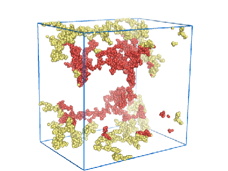
Figure 2: Example of an initial structure used for the simulations. A fractal cluster is grown using particle diffusion kinetics and then allowed to relax to a local minimum under the effect of the particle interactions. We use periodic boundary conditions and only clusters percolating in all three spatial directions are retained. The main cluster is shown in dark gray (red online), whereas slices of periodic copies are reproduced in light gray (yellow online) in order to allow to see the percolating structure.

Although the interaction potential given by Eq. (1) is potentially compatible with gel-like structures, it is evident that the cluster produced by the DLCA-DEF construction will in general be far from an energetic optimum since it does not take into account the particle interaction and in particular we must expect to find particles at, or close to, the unfavourable distance $R_{max}$ corresponding to the potential barrier. Using the DLCA-DEF cluster directly as an initial configuration for a MD run at constant energy with the interaction potential given by Eq. (1) would therefore very likely lead to a quick disintegration of the cluster.

In order to avoid this problem we first allowed the DLCA-DEF cluster to adapt to the interaction between particles by letting it relax toward a (local) energy minimum. In practice this was done by running a MD simulation at zero temperature (using a time step of $h=0.001$), thereby allowing unfavorably placed particles to adapt their positions before starting the actual simulations. We found that in general the overall fractal, open structure of the cluster remains unaffected by this process (details of structural changes at this stage will be discussed below), and only rarely the relaxation led to the breaking of a chain, in which case the resulting structure was discarded. We also discarded the configuration in the case where this adaptation led to a loss of percolation in any spatial direction. In Fig. 2 we show a typical resulting cluster used as initial configuration for the MD simulations at constant temperature.

Molecular Dynamics

Using the relaxed clusters as initial configurations, we carried out molecular dynamics simulations to study their structural evolution at various temperatures ($T=0.05$, $0.10$, $0.15$, $0.20$, $0.25$, $0.30$, $0.35$, $0.40$, $0.45$, $0.50$, $0.55$ and $0.65$). Furthermore we investigated dynamic quantities. Since at the start of the simulation the system is out of equilibrium one has to use two-times quantities in order to characterize the relaxation dynamics [14], which depend on both the waiting time $t_{w}$ (also called the “age of the system”, which is the time which has elapsed between the initial zero-temperature adaptation of the cluster and the beginning of the dynamical measurement), as well as the time lag $\tau$ since the beginning of the dynamical measurement.

As already mentioned, we use $\sigma$ and $\epsilon$ as units of length and energy, respectively. Temperature is thus measured in units of $\epsilon$, whereas time is measured in units of $\sqrt{\sigma^{2}m/\epsilon}$, with $m$ being the mass of a particle.

We use the standard velocity-Verlet algorithm [22] to propagate the system in phase space. Since it is out of equilibrium, coupling it to a heat bath is required in order to prevent it from heating up. We use a variant of Andersen’s thermostat [22] by randomizing periodically all velocities according to the appropriate Maxwell-Boltzmann distribution (in practice every $\Delta_{therm}=0.25$ time units). Thus this type of dynamics is Newtonian for short times, but resembles Brownian dynamics for times longer than $\Delta_{therm}$. For computational efficiency the interaction potential is truncated and shifted at a cutoff radius of $R_{c}=2.58$. All simulations were carried out with a time step of $h=0.005$, except for intervals of duration $\Delta_{therm}$ after selected waiting times, where a time step of $h=0.001$ was used in order to improve the resolution for the mean square displacement (see below).

In order to improve the statistics of the results, we have furthermore averaged over ten runs with independent initial configurations.

3 Structure

We start the discussion of the properties of the gel by considering its structure and its evolution as a function of the waiting time $t_{w}$.

Radial distribution function

We first of all analyze the distribution of inter-particle distances, through the radial distribution function $g(r)$, defined as [23]

$$g(r)=\frac{1}{4\pi r^{2}\rho N}\sum_{k}\sum_{j\neq k}\langle\delta(r-|\vec{r}_{j}-\vec{r}_{k}|)\rangle\quad.$$ (3)

The inset in Fig. 3, shows the radial distribution function of the original DLCA-DEF structure, i.e. before the zero-temperature adaptation to the interaction potential given by Eq. (1). We see that the first nearest neighbor peak at $R_{min}\approx 1.29$ is very high and narrow, as is to be expected in view of the DLCA-DEF algorithm used to construct the structure. Furthermore we notice that $g(r)$ is non-zero for all distances larger than $R_{min}$ and that there are distances at which singularities arise, e.g. around $r=2.5$. These features are also directly related to the algorithm, and they highlight that the DLCA-DEF structure is very different from that of simple liquids such as hard spheres or Lennard-Jones particles.

In the main panel of the figure we show the radial distribution function at $t_{w}=0$, i.e. immediately after the DLCA-DEF structure has been allowed to relax to the nearest minimum of the potential given by Eq. (1). At this stage the structure has changed significantly and several peaks are present, which we have labelled by the local particle configurations responsible for these peaks. Due to the low dimensionality of the structure, this correspondence can be established up to relatively large distances, unlike what is the case in dense simple liquids. We may furthermore deduce from this figure that particles have been expelled from the inter-particle distance corresponding to the position of the repulsive barrier ($R_{max}\approx 1.8$), as is witnessed through the drastical suppression of $g(r)$ around these values. In this sense, too, the local structure of our model gel is therefore very different from a simple liquid. In the following the presence of this gap in $g(r)$ will allow for a straightforward definition of first nearest neighbor pairs in the following.

Finally we point out that the location of the main peak is at $r\approx 1.33$, i.e. at a distance slightly larger than the location of the minimum in $V(r)$ (which occurs at $R_{min}\approx 1.29$), implying that the system is under weak tension, i.e. that the pressure is negative.

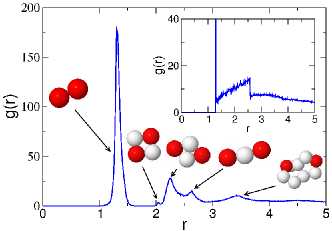
Figure 3: The radial distribution function, $g(r)$, corresponding to the fractal clusters after initial adaptation to the interaction potential. The main peaks are labeled by the corresponding local particle arrangements, the distance $r$ referring to the separation between particles displayed in dark gray. For comparison, the inset shows $g(r)$ for the configurations obtained from the DLCA-DEF algorithm, i.e. before adaptation to the potential.

Static structure factor

Complementary information on the structure can be obtained from the static structure factor $S(q)$ which is given by [23]

$$S(q)=\frac{1}{N}\sum_{j}\sum_{k}\exp[i\vec{q}\cdot(\vec{r}_{j}-\vec{r}_{k})]\quad,$$ (4)

where $q=|\vec{q}|$ is the modulus of the wave-vector. The $q-$dependence of $S(q)$ is presented in Fig. 4 where we compare the static structure factors for the DLCA-DEF cluster before the zero-temperature relaxation with the one after the relaxation. We see that the small wave-vector regimes are identical within the noise of the data, and thus we conclude that the relaxation process has not changed the large scale structure of the cluster. On these length scales the $q-$dependence is described well by a power-law, $S(q)\sim q^{-d_{f}}$, with an exponent $d_{f}\approx 1.8$. This confirms that the system is fractal, as is the case for experimentally observed colloidal gels [16, 24]. Effects of the zero-temperature relaxation are visible at intermediate and large wave-vectors ($q\geq 1$) showing that rearrangements arise on the scale of a few particles, in agreement with the conclusions from $g(r)$. However, the differences in $S(q)$ are much less pronounced than the ones found in $g(r)$ (see Fig. 3), which shows that in this case the radial distribution function is more sensitive to the modifications than the static structure factor. From Figs. 3 and 4 we can conclude that the structure of the DLCA-DEF clusters as well as the relaxed clusters form an open and percolating network structure with a fractal dimension, which is compatible with the structure found in real colloidal gels [16].

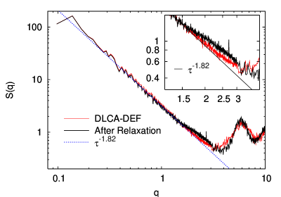
Figure 4: Static structure factor as function of the wave-vector. The thin and bold lines are for the DLCA-DEF and the relaxed structures, respectively. The power-law fit yields the fractal dimension. The inset shows an enlargement at intermediate $q$ in order to illustrate the change of the structure on the scale of the filament thickness, i.e. several particle diameters.

The zero-temperature adaptation to the interaction potential can, however, only be expected to produce a metastable structure, which will evolve with time. In the following we therefore discuss the waiting time dependence of $S(q)$. In Fig. 5 we show $S(q)$ for a waiting time $t_{w}\approx 75000$. The different curves correspond to different temperatures and we see that $S(q)$ for low $T$ is very different from the one at high $T$. The structure for the lowest temperatures has not changed much from the relaxed initial configuration, despite this long waiting time, suggesting that the structure is essentially frozen at these $T$ and $t_{w}$. This changes with increasing $T$, curves for $T=0.25$ and $T=0.3$, where the amplitude of $S(q)$ at low $q$ decreases rapidly, which shows that the large scale structure starts to change significantly. The structure at intermediate and large wave-vectors is, however, much less affected by this increase of $T$. Thus we can conclude that the large scale structure of the network has broken up, whereas the local structure is still relatively ‘intact’ as compared to the initial structure of the relaxed cluster. As temperature is increased even further the structure factor becomes essentially flat, i.e. the network structure of the system has broken up completely into a gas of particles and small clusters.

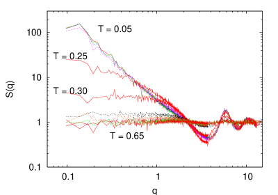
Figure 5: Static structure factor $S(q)$ after the waiting time time $t_{w}\approx 75000$ for all temperatures considered ($T=0.05,...,0.65$, with an increment of $0.05$). For moderate temperatures the fractal structure is lost on large scales, but remains intact over intermediate distances. For higher temperatures, all structure is lost as the initial cluster decomposes into a gas of particles and small clusters.

Figure 6: a) Number of clusters vs. waiting time, illustrating the breakup of a single, percolating cluster, for various temperatures. b) The same quantity as in a) but now normalized such that at $t_{w}\to\infty$ all the curves converge to 1.0.

Cluster statistics

The aging of the structure can also be analyzed by considering $n(t_{w})$, the number of clusters in the system as a function of the waiting time, as shown in Fig. 6 for medium and high temperatures ($T\geq 0.20$). For $t_{w}=0$ we have a single (percolating) cluster. Then $n(t_{w})$ increases with the waiting time $t_{w}$, and the associated time-scale strongly depends on temperature, see Fig. 6a. Finally the number of clusters $n(t_{w})$ saturates for large $t_{w}$, showing that the system has completely relaxed, and the saturation value of $n(t_{w})$ indicates the number of clusters in equilibrium. Note that the saturation value $n(t_{w}\to\infty)$ depends on temperature, since most of the particles are isolated at high $T$ whereas they prefer to form clusters at low $T$.

Figure 6a suggests that the shape of $n(t_{w})$ is independent of temperature, such that the only effect of temperature would be a change in the relaxation time. In order to test this we consider the number of clusters (minus one), normalized by its long time limit:

$$\frac{n(t_{w})-1}{n(t_{w}\to\infty)}\quad.$$ (5)

Note that this is of course only possible for those temperatures for which there is a long-time plateau in Fig.6a, i.e. for $T\geq 0.3$.

This quantity is shown as a function of $t_{w}$ in Fig. 6b, confirming that the shape of the normalized curves is indeed only a very weak function of $T$. Furthermore we can conclude that the initial increase of $(n(t_{w})-1)/n(t_{w}\to\infty)$ is approximately a power-law with an exponent close to 0.5. Although we do not have a complete explanation for this particular exponent, it does demonstrate that the initial increase is not exponential, as would be expected for a process in which the initial cluster breaks up on a fixed time-scale $\tau_{break}$ into sub-clusters, which in turn break up into subclusters, etc., with a fixed time-scale for breakup. On the contrary, Fig. 6b suggests that clusters break up in a heterogeneous manner regarding sizes and time scales.

As mentioned above, the initial percolating cluster disintegrates into smaller clusters and reaches an equilibrium for long times. Beyond the asymptotic value of the number of clusters already mentioned above, we can also analyze the breakup in terms of the evolution of the cluster distribution $P(s)$ as a function of cluster size $s$. $P(s)$ depends on temperature (and at short and intermediate times also on $t_{w}$). In Fig. 7 we present $P(s)$ at $T=0.4$ for various waiting times $t_{w}$. For $t_{w}=0$ the cluster size distribution has a single peak at $s=N$, corresponding to the initial percolating cluster. Even for small $t_{w}$ the distribution very quickly flattens out, i.e. all cluster sizes become essentially equally likely (see curve for $t_{w}=16$). As $t_{w}$ is increased further the proportion of small clusters increases quickly whereas that of large clusters diminishes. For sufficiently long times, i.e. when the system has equilibrated, the (asymptotic) distribution function is described well by an exponential (solid line), since the particles just form random aggregation clusters which follow Poisson statistics. Below we will make use of this result when we discuss the relaxation dynamics of the system.

Figure 7: Cluster size distribution for high temperature ($T=0.40$), represented for various ages. $P(s)$ is the probability of finding a cluster consisting of $s$ particles in the system. Initially only one big cluster is present, which decomposes progressively. The final regime is stationary (the last two curves for large ages superpose), and are well described by an exponential distribution, solid line, as one would expect in a gas of attractive particles.

4 Relaxation Dynamics

After the discussion of the static structure of our model gel, we now focus on its dynamical properties. As we will see below, for intermediate and low temperatures, one can distinguish three time regimes: (i) For $t_{w}$ much shorter than the time scale for the breakup of the percolating cluster, the behavior is dominated by vibrational and quasi-elastic effects. (ii) This is followed by a regime in which the system ages strongly as its structure changes while the percolating cluster breaks up. (iii) Finally, at very long times, the system has reached equilibrium and we thus observe the relaxation dynamics of a system consisting of small clusters. Although these three regimes are also reflected in the time evolution of structural quantities, such as the number of clusters shown in Fig. 6a, we will show that the aging of the system affects the time correlation functions much more strongly than the static quantities, in agreement with previous investigations on glass-forming systems out of equilibrium [25]. We will first analyze the average mean squared displacement of the particles to extract information on the diffusive (or non-diffusive) nature of the dynamics, before presenting a complete study of the self-intermediate scattering function, and reporting on the spatio-temporal characteristics of the relaxation processes.

4.1 Mean squared displacement

Since we are dealing with an out-of-equilibrium situation, the usual mean squared displacement (MSD) has to be generalized by explicitly taking into account the time at which the measurement is started. We thus define

$$\Delta^{2}(t_{w},t_{w}+\tau)=\frac{1}{N}\sum_{i=1}^{N}\langle(\vec{r}_{i}(t_{w}+\tau)-\vec{r}_{i}(t_{w}))^{2}\rangle\qquad.$$ (6)

Since in aging glass-forming systems the relaxation dynamics has been found to slow down with increasing $t_{w}$ [14] we may expect the same behavior in the present system. However, before addressing this point it is useful to discuss the temperature dependence of $\Delta^{2}(t_{w},t_{w}+\tau)$ . To this end we select a waiting time which is relatively long, $t_{w}=13446$, and show in Fig. 8 $\Delta^{2}(t_{w},t_{w}+\tau)$ for different temperatures. At short times $\tau$ we find the ballistic behavior, $\Delta^{2}(t_{w},t_{w}+\tau)\propto\tau^{2}$ (dashed-dotted line) as it is seen for all systems with Newtonian dynamics. This ballistic regime ends at $\tau=0.25$, the time at which the thermostat acts for the first time.

Temperature dependence

At high temperatures, $T=0.65$, this ballistic regime immediately crosses over into a diffusive regime, $\Delta^{2}(t_{w},t_{w}+\tau)\propto\tau$ (dotted line in Fig. 8). A look at Fig. 6 shows that for this temperature and at this waiting time the initial percolating gel has already fallen apart into many small clusters which have completely equilibrated, and the observed $\Delta^{2}(t_{w},t_{w}+\tau)$ is therefore just the MSD of the disintegrated system consisting of clusters in equilibrium.

Figure 8: Mean squared displacement $\Delta^{2}(t_{w},t_{w}+\tau)$ of the particles as a function of time $\tau$ for different temperatures, for $t_{w}=13446$. Also included are power-laws found in the ballistic regime at small $\tau$ (dash-dotted line), in the diffusive regime at large $\tau$ (dotted line), and in the sub-diffusive regime (solid line).

At low temperatures, on the other hand, the MSD shows a different $\tau-$dependence once the ballistic regime is over. In this case the MSD is sub-diffusive and can be well approximated by the power-law $\Delta^{2}(t_{w},t_{w}+\tau)\propto\tau^{\alpha}$ with an exponent $\alpha$ around 2/3 (solid line). Note that for sufficiently low temperatures $T$ this exponent appears to be independent of temperature: the curves for $T=0.15$ and $T=0.05$ are parallel, and it is only for intermediate temperatures, $T=0.3$, that the exponent of the sub-diffusive regime exceeds 2/3. We observe furthermore that at this $T$ this sub-diffusive regime ends at around $\tau\approx 10^{4}$ where the MSD starts to bend upwards, and from here on it grows proportionally to $\tau$, which we rationalize as follows. A comparison with Fig 6 shows that, at this temperature, the system starts to show significant aging effects on the time scale of $\tau\approx 10^{4}$, i.e. the number of clusters is already relatively large although it has not yet reached the final (equilibrium) distribution. It can be expected that many of these clusters are relatively small and consequently move fast. Since the (average) MSD is dominated by fast moving entities, it is therefore not surprising that at $\tau\approx 10^{4}$ the MSD already shows diffusive behavior even though the system is not in equilibrium yet.

Last but not least, we point out the absence of plateaus in the MSD in Fig. 8 at intermediate time scales. Such a plateau is a typical feature of most glass-forming systems at high density [14], where it is related to the so-called cage effect, i.e. the temporary trapping of a particle by its surrounding neighbors. In contrast to this the present gel has the structure of a very open network, cf. the snapshot in Fig. 2. Whereas in this system the cage effect may indeed be expected to be present along the chains, we may conclude that the particle movements from transverse motion, ie. orthogonal to the chains, is sufficiently strong as to mask the plateau in the MSD, in agreement with previous findings [3, 10, 29].

Waiting time dependence

We now turn to the waiting-time dependence of the MSD. In Fig. 9 we show the $\tau-$dependence of $\Delta^{2}(t_{w},t_{w}+\tau)$ for different waiting times $t_{w}$, all at a relatively high temperature of $T=0.4$, allowing us to study the behavior of $\Delta^{2}$ in the aging regime as well as in equilibrium (see Fig. 6). For short waiting times, $t_{w}=4$, we see that after the ballistic regime (not shown in the figure) $\Delta^{2}$ shows a $\tau-$dependence which is compatible with $\tau^{2/3}$, i.e. the same power-law which we have found for the MSD at low temperatures and long waiting times (see Fig. 8). Thus we can conclude that this sub-diffusive behavior is not only limited to low temperatures, but can be observed at all temperatures in the time window which corresponds to the onset of aging. In contrast to this for intermediate times $\tau$ the MSD is super-diffusive, and compatible with a power-law with exponent $\alpha\approx 1.5$. This behavior arises in the time regime in which the structure of the system changes rapidly, leading to the complete breakup of the gel (see Fig. 6). At even longer times the MSD shows simple diffusive behavior, i.e. $\Delta^{2}\propto\tau$.

Figure 9: Mean squared displacement at $T=0.40$ for different waiting times $t_{w}$. Note that for reasons of clarity we do not show the ballistic regime present at very small times ($\tau<0.25$). Also included are power-law fits with exponent 1.0, characterizing the diffusive regime seen for $t_{w}=72317$, as well as with exponents 2/3 and 1.5 characterizing the MSD at small $t_{w}$ at short and long times $\tau$, respectively.

For a larger waiting time, $t_{w}=464$, the MSD no longer shows the intermediate $\tau^{2/3}$ behavior seen for intermediate times; instead we observe a power-law with an exponent between 2/3 and 1.0. On the other hand, the long time behavior is again compatible with a $\tau^{3/2}$ behavior for the MSD. Thus we can conclude that for this waiting time the initial relaxation dynamics is faster than that for short waiting times, and once the initial structure of the system has changed significantly it once more shows the same super-diffusive dynamics as for small $t_{w}$. Finally, for a long waiting time, $t_{w}=72317$, the MSD enters the diffusive behavior right after the initial ballistic regime, which is expected for a system in equilibrium at long times. In summary, we thus observe that, after the initial ballistic regime, the MSD of the system shows a power-law with exponent of roughly 2/3 at an intermediate time window, as long as the gel has not yet undergone major restructuring with respect to its initial state. At intermediate times, as the structure starts to change significantly, the MSD shows a super-diffusive power-law with an exponent around 3/2. Finally, for very long times, the MSD shows the linear $\tau-$dependence found in equilibrium systems.

Figure 10: Mean squared displacement at $T=0.05$ for different waiting times $t_{w}$. Note that for reasons of clarity we do not show the ballistic regime present at very small times ($\tau<0.25$). Also included is a power-law fit to the MSD for large $t_{w}$ with an exponent 2/3.

For the sake of completeness we also show the $\tau-$dependence of the MSD at low temperature ($T=0.05$) and different waiting times, see Fig. 10. For large waiting times we again find a power-law with an exponent around 2/3. However, for smaller waiting times, $t_{w}\leq 464$, the MSD shows a small (positive) deviation from this power-law at intermediate times. The reason for this is probably the fact that at $t_{w}=0$ the structure is under weak tension (see the discussion in the context of Fig. 3), so that the resulting forces lead to a somewhat faster relaxation dynamics than what is observed at large waiting times, for which the tension has already relaxed.

Dynamics of particle chains

We devote the following paragraphs to the discussion of the mechanisms which may give rise to a power-law dependence of the MSD with an exponent around 2/3, which we have pointed out in various time windows (Figs. 9 and 10). In particular, we explore the role of the dynamics of particle chains forming the gel network. We recall that, at short and intermediate times, the dynamics of the nodes in the gel network is much slower than the transverse fluctuations of the chains. We may thus hope to understand the anomalous $\tau-$dependence of the MSD by considering “clamped” individual chains, i.e. chains with endpoints that are fixed in space.

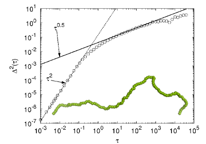
Figure 11: Mean squared displacement $\Delta^{2}(t_{w},t_{w}+\tau)$ of a single chain whose endpoints are clamped at a distance $L=R_{min}N$. $T=0.05$ and $N=100$. The solid lines are fits with power-laws $\tau^{2}$ for short times and $\tau^{0.5}$ at intermediate times. Note that the chains have been equilibrated before starting the calculation of the MSD and hence $\Delta^{2}$ does not depend on $t_{w}$. Inset: Snapshot of a clamped equilibrated chain of $N=100$ particles with length $L=0.6R_{min}N$, obtained at $T=0.05$.

To this end we have performed MD simulations of isolated chains of particles. As starting configurations we used individual straight linear chains of $N=100$ particles placed at their preferential distance $R_{min}\approx 1.29$, which thus have a total length of $L=R_{min}N$. Apart from holding the chain ends fixed, all other simulation details (time step, heat bath, etc.) were identical to those used for simulating the entire gel. The chains were thermalized at $T=0.05$ before starting to acquire data for the MSD. In order to improve the statistics of the results we have done 10 independent runs.

In Fig. 11 we show $\Delta^{2}(\tau)$ as a function of $\tau$ (note that, since this is a system in equilibrium, the MSD does not depend on the waiting time, and we therefore omit the variable $t_{w}$). At short times we have $\Delta^{2}(\tau)\propto\tau^{2}$ (ballistic regime), whereas for long times $\Delta^{2}(\tau)\propto\tau^{1/2}$, as is expected for a Rouse chain [26]. For very long times the MSD saturates, since the chain is clamped at its ends which in turn limits the displacement of particles in the chain to a certain distance which depends on $L$, $N$, and $T$. The small oscillations seen at $\tau\approx 10^{4}$ are also related to the clamping through fixed endpoints, since they are due to the excitation of the fundamental mode of the chain. Last but not least we point out that the mentioned Rouse behavior is in fact not expected to be observable for chains that are not very long, since it is known that for free short chains the exponent 0.5 in the power-law is replaced by an exponent around 0.6-0.7 [27]. Since in our gel the length of the connecting chains is not very large, see Fig. 2, it can be speculated that the exponent 2/3 found at short waiting times is related to the relaxation dynamics of such (short) chains. However, below we will discuss other mechanisms which potentially explain the observed behavior.

Figure 12: The exponent $\alpha$ defined via $\Delta^{2}(t_{w},t_{w}+\tau)\propto\tau^{\alpha}$ as a function of the end-to-end distance of a clamped chain. $T=0.05$. See text for a detailed description of how the initial configurations have been prepared. Note that the chain has been equilibrated and hence the $\Delta^{2}$ does not depend on $t_{w}$. The point labeled “Free end chain” corresponds to a chain in which only one end was fixed, i.e. the value of the abscissa is irrelevant.

The chains considered so far were not under tension, i.e. the distance between the fixed ends was given by $L=R_{min}N$. In reality, however, we have found the chains of the network to be under weak tension (see the discussion in the context of Fig. 3), and it is therefore of interest to determine the extent to which the presence of such a tension modifies the relaxation dynamics. We have therefore performed simulations in which the distance between the end points of the chain were fixed at $L$ which differed from $N\,R_{min}$. A typical snapshot of such a chain is shown in the inset of Fig. 11. For all cases we have found that at intermediate and long times the MSD is given by a power-law with an exponent $\alpha$ (and for very long times the MSD of course saturates). In Fig. 12 we show the $L-$dependence of this exponent and we see that for strongly compressed chains, $L<0.7<R_{min}$, $\alpha$ is around 2/3. This limiting value can be rationalized by the fact that most of the monomers of a significantly compressed chain will not really feel that the ends of the chain are held fixed, and therefore the MSD will behave very similarly to a semi-free chain. In order to determine the value of $\alpha$ for such a semi-free chain, we have run a simulation in which only one end of the chain was kept fixed and, see Fig. 12, we find that such a chain indeed gives rise to an exponent $\alpha=2/3$.

If the distance between the ends of the chain is increased to $L=R_{min}N$, on finds the exponent $\alpha=0.5$, in agreement with the result shown in Fig. 11. If the chain is extended even further, $L>R_{min}N$, the exponent becomes smaller than 0.5. Thus we can conclude that a chain which is not clamped at its equilibrium length shows a relaxation dynamic which differs from Rouse chain dynamics.

In order to check to what extent these results depend on the number of monomers in the chain we have included in Fig. 12 also the exponents for a chain of length $N=200$. We see that this dependence is not strong, in that the two curves are essentially identical for chains at their equilibrium length, stretched chains or significantly compressed chains. The only appreciable difference arises for slightly compressed chains ($L/NR_{min}$ somewhat smaller than 1.0), for which the exponent appears to increase with chain length. This effect is due to the fact that a longer chain will allow the particles far away from the ends to undergo a relaxation dynamics which is less constrained than in shorter chain, i.e. the dynamics is more similar to a free chain, for which the exponent is 2/3.

Figure 13: Mean squared displacement $\Delta^{2}(t_{w},t_{w}+\tau)$ for a single clamped chain of $N=100$ particles, obtained at $T=0.05$. After having been equilibrated, the chain, keeping its endpoints fixed, is artificially cut in the middle at time $\tau=100$. Note that the ballistic part is not shown.

In addition to the clamped chains we have also considered chains that break up, as we must expect to happen naturally in the gel structure, in order to study the contribution of such chain-breaking to aging. For this we have used the equilibrated chains discussed above and started an equilibrium simulation at time $t_{0}$. At time $t_{0}+100$ the chains were then artificially broken in the middle and we have followed their out of equilibrium dynamics from this point on. Figure 13 shows the MSD for different waiting times $t_{w}$. The data for $t_{w}=0.001$ shows a crossover, at short times, from the ballistic regime to the dynamics shown in Fig. 11 which follow the $\tau^{0.5}$ power-law. At $\tau=100$, the time at which the chain is broken, this regime is interrupted and the MSD shows a super-diffusive dynamics before it appears to slowly approach an asymptotic behavior. This asymptotic long-time regime is more readily deduced from the data for longer waiting times, see curve for $t_{w}=36896$, for which the overall time which has elapsed since the chain was broken is much larger. Consequently, although the behavior for small $\tau$ is as just described, the asymptotic regime is attained over a much longer interval, and we may deduce that the long-time chain relaxation of a broken chain is compatible with a power-law $\Delta^{2}\propto\tau^{2/3}$. For even longer times $\tau$, not easily accessible in our simulations, the MSD must of course saturate again. We can therefore conclude that the out of equilibrium relaxation of a chain following breakage obeys a power-law with exponent 2/3. Consequently, chain breakage constitutes another potential explanation fore the a $\tau-$dependence of MSD observed in the model gel.

In summary one can conclude that the exponent 2/3 observed in the MSD for the system at low temperatures and long waiting times can have at least three origins: (i) rare ruptures of chains in the network, (ii) large transverse fluctuations of floppy clamped chain-like filaments, and (iii) fluctuations of dangling filaments. Currently we have not attributed the anomalous diffusion effects to a dominant contribution from either of these mechanism, which may in principle all coexist.

4.2 Self-intermediate scattering function

In order to obtain more detailed information on the relaxation processes, in particular regarding the length-scale at which they occur, we have investigated the self-intermediate scattering function [23] generalized to a two-time quantity:

$$F_{s}(q,t_{w},t_{w}+\tau)=\frac{1}{N}\sum^{N}_{j=1}\langle\exp[i\vec{q}\cdot(\vec{r}_{j}(t_{w}+\tau)-\vec{r}_{j}(t_{w}))]\rangle\quad.$$ (7)

Here we have assumed that the system is isotropic and therefore $F_{s}$ depends only on $q=|\vec{q}|$. Recall that this function can be measured experimentally via scattering techniques [24], and therefore it is not only of theoretical interest but allows also to compare the results from simulation with experimental data.

Since the relaxation dynamics at high temperature (where we have interrupted aging [14]) is very different from the one at low temperatures, we discuss them in two separate subsections.

4.2.1 High temperature regime

Figure 14: Time dependence of the generalized self-intermediate scattering function $F_{s}(q,t_{w},t_{w}+\tau)$ at a high temperature ($T=0.4$). The waiting times are $t_{w}$ = 0.001, 4, 16, 44, 86, 237, 464, 1275, 4900, 13446, 26354, 51655, and 72317. Note that the relaxation time decreases with increasing age.

In Fig. 14 we show the $\tau-$dependence of $F_{s}(q,t_{w},t_{w}+\tau)$ for $T=0.40$, i.e. a temperature at which we can see strong aging of the system, but which is still sufficiently high to allow reaching equilibrium within the time span of the simulations, see Fig. 6 (higher temperatures give a qualitatively similar relaxation dynamics). Data are shown for two wave-vectors: $q=0.24$, corresponding to a distance which is about 20 times larger than the typical nearest-neighbor distance (first peak in the structure factor, see Fig. 5), and $q=2.41$, corresponding to 2-3 particle diameters. For each of these wave-vectors we show several curves, which correspond to different waiting times. One sees immediately that the shape of the curves as well as the associated relaxation time depends on the age of the system, and in the following we will discuss this dependence in more detail. Even without any detailed analysis it is, however, evident that the relaxation dynamics accelerates with the sample age, as is expected from the picture of an initially percolating structure which disintegrates through clusters breaking up into ever smaller clusters, which in turn break up themselves etc. Note that this $t_{w}-$dependence is different from the one found in dense aging glass-formers, for which the relaxation time increases with age [14].

In order to discuss the $q$ and $t_{w}$ dependence of the relaxation dynamics we have fitted $F_{s}(q,t_{w},t_{w}+\tau)$ with a Kohlrausch-Williams-Watts (KWW) function, $A\exp(-(\tau/\tau_{f})^{\beta})$, using the time range in which the time correlation function has fallen below 0.8. Although there is no theoretical justification for this functional form, we have found that the fits are indeed very good, and consequently the parameters $\tau_{f}(q,t_{w})$ and $\beta(q,t_{w})$ can be used to characterize the relaxation time and the stretching of the dynamics.

Figure 15: Wave-vector dependence of the KWW exponent $\beta$ at a high temperature ($T=0.4$). The waiting times are $t_{w}$ = 0.001, 4, 16, 44, 86, 237, 464, 1275, 4900, 13446, 26354, 51655, and 72317. Note that at small and large $t_{w}$ the curves depend only weakly on $t_{w}$ whereas a significant $t_{w}-$dependence is seen at intermediate waiting times.

Stretching exponent

In Fig. 15 we show the wave-vector dependence of the KWW exponent $\beta$ for different waiting times. At short waiting times, $t_{w}\leq 86$, the curves depend only weakly on $t_{w}$, since on this time scale the gel ages only weakly. For intermediate times, however, $\beta$ depends strongly on $t_{w}$, since the system ages significantly in this regime. Finally, for large $t_{w}$, the different curves fall onto a master curve which describes the equilibrium dynamics of the system. Note that at small waiting times the KWW exponent $\beta$ depends quite strongly on $q$: We have $\beta\approx 1.2$ at large length scales, which corresponds to a so-called compressed exponential, whereas $\beta\approx 0.4$ at small length scales, corresponding to a strongly stretched exponential. We attribute this $q-$dependence to the fact that the network structure is still intact at short $t_{w}$, such that the high temperature imposes strong deformations on the filaments, and therefore strong tensions. Such stresses ultimately lead to an elastic relaxation at a large scale (small $q$), which superposes and dominates diffusive relaxation. Such a compressed exponential, with exponent $\beta=3/2$, has indeed been predicted from an internal stress model [13, 16]. A more refined microscopic approach [28] has lead, under certain conditions, to predictions of $\beta=5/4$, which is indeed close to the exponents represented in Fig. 15 at small $q$, corresponding to length-scales on which one may hope that concepts of elasticity apply.

We can furthermore rationalize why $\beta$ is small for large wave-vectors and short $t_{w}$, by recalling that the short-time structure of the system must locally retain some frustration, since it has been created by what is essentially a steepest descent procedure in the potential energy. The resulting local geometry is therefore very heterogeneous and includes regions with high stress and others with low stress, and which thus will relax on quite different time-scales. We may therefore expect the average relaxation dynamics to be a function which extends over many time scales and which can be well fitted with a KWW function with a small $\beta$. For long times, on the other hand, these local stresses have successively homogenized, and therefore the typical relaxation times no longer cover a large time window: the KWW exponent increases, in agreement with what is seen in Fig. 15.

Interestingly, a strong $q-$dependence of the exponent $\beta$ has also been observed in experiments of aging gels [12] as well as in simulations of gels in equilibrium [29]. These experiments show that, at small $q$, the stretching exponent $\beta$ is indeed larger than unity and decreases as a function of the wave-vector. This dependence is thus qualitatively similar to the one found in the present study. However, in the simulations of Ref. [29] the trend is opposite, i.e. where $\beta$ increases with $q$, and consequently we have $\beta>1$ only at large wave-vectors. The reason for this difference probably resides in the fact that in the latter work the microscopic dynamics was entirely Newtonian, i.e. there was no coupling to a heat bath as in the present simulation. Consequently the particles could follow a ballistic motion at small length-scales, whereas such a time dependence is not possible here due to the presence of the thermostat (which mimics the solvent of a real system, in a rough way). Furthermore, caution is in order when drawing parallels with the dynamics of a gel in equilibrium, such as the one studied in Ref. [29], since it is very different from the out-of-equilibrium dynamics considered here.

Figure 16: Aging time dependence of the Kohlrausch exponent $\beta$ at a high temperature ($T=0.4$). The different curves correspond to different wave-vectors.

In Fig. 16 we show the age dependence of the Kohlrausch stretching exponent for different length-scales identified through $q$, all at $T=0.4$, in order to understand how aging affects the dynamics on different length-scales. For very short times the exponent $\beta$ is constant for all $q$, i.e. the out-of-equilibrium situation of the system does not yet affect its relaxation dynamics. For intermediate times $\beta$ decreases, i.e. the dynamics becomes more stretched, and from the data we see that the time window in which this decrease is observed depends strongly on $q$. For large wave-vectors the increase of the stretching is observed very early and followed by a zone of roughly constant $\beta$ for intermediate times ($10^{1}\leq t_{w}\leq 10^{3}$). For small $q$, in contrast, the decrease of $\beta$ starts only at around $t_{w}\approx 10^{2}$ and stops at $t_{w}\approx 10^{4}$. These results are quite reasonable since the relaxation times strongly decrease with the wave-vector $q$ (see Fig. 17). Consequently, aging will affect the relaxation dynamics first on a small length-scale, and only later on a large length-scale.

For even larger times the structure starts to break up and hence $\beta$ increases again. This acceleration is seen first at large wave-vectors, since the system will equilibrate faster on small length-scales than on large ones. For very long waiting times the exponent $\beta$ becomes independent of $t_{w}$, since the system has equilibrated, and converges to a value smaller than unity. In the Appendix we show that this limiting value (around $\beta\approx 0.8$) can be directly deduced from the equilibrium distribution of the cluster size shown in Fig. 7.

Figure 17: Relaxation time $\tau_{f}$ as a function of the age of the system for different wave-vectors $q$ ($q=0.17,0.31,0.49,0.80,1.22,1.82,2.41,3.50,4.88,$ and $5.89$, top to bottom). The temperature is $T=0.4$.

Relaxation time

We now turn to the relaxation time $\tau_{f}$ and discuss its dependence on waiting time and wave-vector. In Fig. 17 we show $\tau_{f}$ as a function of $t_{w}$ for different wave-vectors. In agreement with the results for the stretching exponent, we see three different regimes: (i) For short waiting times $t_{w}$ the relaxation time $\tau_{f}$ is constant. (ii) For intermediate $t_{w}$ the relaxation time starts to decrease; note that the time at which this decrease is seen depends significantly on $q$ and occurs much earlier for the short length scales. (iii) Finally the relaxation time becomes independent of $t_{w}$ since the system has reached equilibrium. The time at which this happens is independent of $q$. Thus we can conclude that the time window in which the aging occurs is large for large $q$ whereas it is relatively narrow for small $q$, which is again in agreement with the findings for the stretching exponent $\beta$.

Figure 18: Wave-vector dependence of the relaxation time $\tau_{f}$ for different waiting times $t_{w}$ at $T=0.4$. In order to check for the presence of the hydrodynamic regime we plot $\tau_{f}q^{2}$.

Finally we discuss the $q-$dependence of the relaxation time $\tau_{f}$. For sufficiently long times we can expect hydrodynamic behavior, and we therefore plot the rescaled relaxation time $\tau_{f}q^{2}$ as a function of $q$, for different values of $t_{w}$, see Fig. 18. The data for short waiting times all collapse onto a master curve if $q$ is small ($q\leq 3$), in agreement with the result shown in Fig. 17, whereas aging is observed only at the largest values of $q$. Note that we do not see a proper hydrodynamic regime in this time window, since the rescaled curves are not flat even at the smallest $q$. This is because the system is still in a gel phase, and hence has a more complex dynamics. For large $t_{w}$, however, we do see the hydrodynamic behavior, i.e. $t_{f}\propto q^{-2}$ at small $q$, and the hydrodynamic regime extends to relatively large wave-vectors. This is probably related to the fact that the asymptotic equilibrium system consists of small clusters, which relax by a simple diffusion mechanism.

4.2.2 Low temperature regime

Figure 19: Time dependence of the intermediate scattering function $F_{s}(q,t_{w},t_{w}+\tau)$ at a low temperature ($T=0.05$). The wave-vectors are $q=2.41$ and $q=0.81$. The different curves correspond to the waiting times $t_{w}$ = 0.001, 4, 16, 44, 86, 237, 464, 1275, 4900, 13446, 26354, 51655, and 72317.

Having discussed the (interrupted) aging dynamics of the system at high and intermediate temperatures, we now address the gel dynamics at low temperatures, at which the system is not able to equilibrate within the time span of the simulations.

In Fig. 19 we show the time dependence of $F_{s}(q,t_{w},t_{w}+\tau)$ at $T=0.05$. Two different wave-vectors are shown, and the different curves correspond to different waiting times $t_{w}$. From this graph we see immediately that the dynamics slows down with increasing $t_{w}$, in contrast to what we have found for intermediate and high $T$ (see Figs. 14 and 17). Thus we can conclude that the aging dynamics at low temperatures is very different from the one seen at intermediate and high temperatures. In particular, it is not possible to interpret the low-temperature dynamics as a special case of the high temperature dynamics at intermediate times, i.e. before the aging is interrupted. This difference can be understood by recalling that the intermediate and high $T$ aging dynamics is dominated by the breakup of the percolating cluster, whereas at low $T$ this cluster stays intact within the simulation time and aging is related to the rearranging of its structure, see Fig. 6.

In order to discuss the details of the $q$ and $t_{w}-$dependence of $F_{s}(q,t_{w},t_{w}+\tau)$ we deduce a relaxation time $\tau_{f}$ and a stretching exponent $\beta$ by fitting the correlator to a KWW-function. The resulting fit characterizes the shape of $F_{s}$ sufficiently well to justify using these parameters, provided we exclude the smallest wave-vectors ($q\leq 0.5$); for these, the correlators $F_{s}(q,t_{w},t_{w}+\tau)$ do not decay significantly for the low temperatures under consideration, and a KWW fit would be clearly inappropriate since the fit parameters would be determined essentially from the short time dynamics and not from the $\alpha-$relaxation.

Figure 20: Waiting time dependence of the relaxation time at $T=0.05$. The different curves correspond to the wave-vectors $q=0.59,0.80,1.22,2.41,4.88,7.50,10.66$, and $15.22$ (from top to bottom).

Relaxation time

The waiting time dependence of the relaxation time $\tau_{f}$ is shown in Fig. 20, for various wave-vectors. We see that for all $q\leq 11$ the dynamics slows down with increasing age, whereas a slight acceleration is observed for the highest $q$. The increase of $\tau_{f}$ with age is the typical behavior found in many glassy systems which are aging. However, in those systems $\tau_{f}(t_{w})$ is usually seen to obey power-law dependence on $t_{w}$, or at least so whenever $t_{w}$ is sufficiently large [14]. This is not really the case for the system studied here, since from Fig. 20 we can conclude that $\tau_{f}$ shows three regimes: (i) At short waiting times the relaxation time is independent of $t_{w}$; the system has not yet had time to react to its changing structure, in agreement with the $t_{w}-$dependence of $\tau_{f}$ found at high $T$ (see Fig. 17). (ii) Subsequently aging starts to modify the structure; the stress present in the initial cluster spreads, but does so without breaking off smaller clusters (see Fig. 6b); this second regime is therefore essentially an elastic relaxation which allows the cluster to accommodate the interaction potential. Note that this regime lasts only for about two decades in time, before it crosses over to (iii) a regime in which, for intermediate wave-vectors, $\tau_{f}$ becomes independent of $t_{w}$. From Fig. 20 we see that the times at which the second regime starts and ends depend quite strongly on $q$, and that for the smallest wave-vector we are not able to see the third regime at all within the time span accessible to the simulation. This is evidence that the stiffening of the structure, which results in an increasing relaxation time, occurs on the local scale before it affects the system on large length-scales. Since the simulated system is rather limited in size, this aging regime does not last very long, and the relaxation times do not increase very much (by less than a factor of five). Although we have not explicitly checked for the presence of finite size effects, we are thus led to think that in the thermodynamic limit the length of the second regime, as well as the increase of $\tau_{f}$, must be much larger than the effects seen in our small sample. This would be in agreement with the experimental findings in real gels [13], for which the sample sizes are much larger than the ones accessible to any simulation.

Figure 21: Relaxation time $\tau_{f}$ as a function of the wave-vector $q$ for $T=0.05$. The different curves correspond to the waiting times $t_{w}=0.001$, 8, 44, 237, 1275, 13446, and 72317.

Figure 22: Relaxation time $\tau_{f}$ times $q^{2}$ as a function of the wave-vector $q$ for $T=0.05$. The different curves correspond to the waiting times $t_{w}=0.001$, 8, 44, 237, 1275, 13446, and 72317 (from bottom to top). The solid curve correspond to a $q^{-3}-$dependence of $\tau_{f}$.

Next we analyze the wave-vector dependence of the relaxation time $\tau_{f}$, which is shown in Fig. 21 for several ages $t_{w}$ ($0.001\leqslant t_{w}\leqslant 72317$). We first consider short waiting times. For intermediate and large wave-vectors we find a $q^{-2}$ scaling for $\tau_{f}(q)$, corresponding to a diffusive motion (dotted line). For small wave-vectors, $q\leq 2.0$, this crosses over to a stronger dependence, and we find approximately $\tau_{f}(q)\propto q^{-3}$ (solid line). For long waiting times, on the other hand, we find that $\tau_{f}(q)$ is given by a power-law $q^{-3}$ in essentially the entire accessible $q$-range (small deviations arise only at the largest $q$). Note that this $q-$dependence implies that the relaxation time on a scale $r$ is proportional to $r^{3}$, and that for a given time scale $\tau$ the particles will therefore reach a typical distance $r(\tau)\propto\tau^{1/3}$. This implies that the mean squared displacement increases like $\tau^{2/3}$, a result that is indeed in agreement with the $\tau$-dependence we have found for the MSD for long waiting times and low $T$, see Fig. 8.

In order to analyze in more detail the diffusive behavior for large wave-vectors $q$ and short waiting times, as identified from Fig. 21, we re-scale the data by plotting $\tau_{f}q^{2}$, see Fig. 22. This confirms that the relaxation dynamics is indeed diffusive on intermediate and large length-scales for short waiting times (bottom curves). For larger waiting times $t_{w}$ the $q$-window for diffusion shifts to smaller wave-vectors and shrinks, finally giving way to a $\tau_{f}\propto q^{-3}$ scaling over the whole accessible $q-$range for the largest waiting times. This graph thus nicely highlights that the relaxation dynamics strongly depends on the wave-vector and on the age considered.

Figure 23: The Kohlrausch exponent $\beta$ as a function of the age $t_{w}$. $T=0.05$. The different curves correspond to different wave-vectors $q$. Note that with increasing $q$ the maximum of $\beta$ moves toward smaller values of $t_{w}$.

Figure 24: The Kohlrausch exponent $\beta$ as a function of the wave-vector $q$. $T=0.05$. The different curves correspond to different ages $t_{w}$.

Kohlrausch exponent

Finally we analyze how the Kohlrausch exponent $\beta$ depends on the wave-vector and on the waiting time. In Fig. 23 we show $\beta$ as a function of $t_{w}$ for different values of $q$. First of all we see that $\beta<1$ for all ages $t_{w}$ and all wave-vectors $q$, i.e. the relaxation dynamics is always stretched. This finding is in contrast to experimental and theoretical results for aging gels, for which compressed exponentials ($\beta>1$) have been reported [16, 13, 28, 29]. One possible explanation for this difference is the fact that the length scales accessible here are much smaller than the ones considered in the experiments or through theoretical arguments. In the cited studies the compressed exponentials have been related to the presence of a local rupture of the network and its subsequent elastic relaxation, which leads to a ballistic motion. An elastic relaxation here means that the part of the gel which has undergone rupture is pulled by a constant force. Due to the presence of the solvent the resulting motion is balanced by a frictional force, and therefore the resulting motion is linear in time, i.e. ballistic. Since in our simulation the network does not break at $T=0.05$ and on the time scales considered, this type of relaxation is not present and hence $\beta<1$. Let us point out that our results are not in contradiction with the results from a computer simulation of a gel in equilibrium mentioned above [29], for which $\beta>1$ was found for large wave-vectors. Since the simulations in Ref. [29] were conducted with Newtonian dynamics (unlike our Brownian-like dynamics due to the thermostat), they trivially give rise to a ballistic motion at small length-scales, which in turn imply a compressed exponential relaxation [28].

¿From Fig. 23 we can further deduce that the stretching at small $t_{w}$ increases continuously with decreasing $q$ (as long as $q$ is not too large), which is evidence that the system becomes increasingly heterogeneous on increasing length-scales. For all values of $q$ we see that, as a function of $t_{w}$, the exponent $\beta$ is essentially constant at small $t_{w}$, then goes through a local maximum before converging to a constant value for large $t_{w}$. Remarkably, this constant of around 0.55 is independent of $q$. The age at which $\beta$ shows its local maximum corresponds roughly to the aging time at which the relaxation time $\tau_{f}(t_{w})$ shows an inflection point, i.e. a strong $t_{w}-$dependence, see Fig. 20. Thus we are lead to conclude that in the time window in which the relaxation time changes significantly (and which depends on the length-scale considered, see Fig. 20) the stretching is weaker than in the regime where the system is not aging quickly. Put differently, rapid aging dynamics is associated with weak stretching, and is probably linked to elastic rearrangements.

Finally we show the wave-vector dependence of $\beta$ for different waiting times, see Fig. 24. For small $t_{w}$, the dynamics is not very stretched at a length-scale corresponding to $q\approx 10$ (pronounced maximum in $\beta(q)$), whereas the stretching is much stronger for $q\approx 1$. With increasing age of the system the maximum in $\beta(q)$ shifts to smaller wave-vectors, i.e. the length-scale on which the system relaxes increases with age. For very long waiting times, $\beta(q)$ appears to converge towards a master function showing a pronounced decrease of $\beta$ at intermediate and large $q$. This master curve is furthermore qualitatively similar to the behavior seen for $\beta(q)$ at higher temperatures, see Fig. 15, where we observe a local maximum around $q=2$, and an increase for smaller $q$’s. The complex shape of $\beta(q)$ seen at long times therefore reflects the relaxation dynamics of the disordered elastic network, in which several relevant length-scales interfere simultaneously.

5 Conclusions

In this article we have studied a system of particles designed to mimic a physical gel. We started from an ad hoc fractal structure, constructed from a modified DLCA algorithm and therefore known to reproduce the structure of dilute, fractal colloidal gels. Although this approach is clearly not inspired by thermodynamics -DCLA-DEF is a purely kinetic algorithm- it has been shown to produce structures which successfully reproduce several measurable quantities of gels, such as the density dependence and the rigidity modulus [21]. It was by no means granted, however, that this way of making a gel-like structure could also be a satisfactory starting point regarding the thermodynamics, left alone the (equilibrium or out-of-equilibrium) dynamics, as we have shown to be the case.

In this study we have investigated the stability of the initial DLCA structure as a physically reasonable particle pair potential is imposed onto the kinetic DLCA structure. Letting the system adapt to this potential, via an initial zero-temperature relaxation, led to significant changes in local ordering while leaving the fractal exponent essentially unaffected. The subsequent relaxation at a given temperature $T$ evolves according to one of the following scenarios.

At high temperature ($T>0.2$), the gel is unstable and ultimately breaks up into small clusters of particles. At low temperature ($T<0.2$) the gel is stable and ages slowly, i.e its aging slows down with observation time.

For high $T$, two regimes for the waiting time must be distinguished. For small $t_{w}$, the self-intermediate scattering function $F_{s}$ is a stretched exponential in time on small length-scales -reflecting the frustrated local structure- and a compressed exponential on large length-scales, where the high temperature imposes strong deformations, such that elastic relaxation dominates. At large $t_{w}$, when the initial structure has decomposed into small pieces, $F_{s}$ is a stretched exponential with essentially a constant exponent $\beta=0.8$ for all wave-vectors, which can be rationalized from the measured long-time distribution of cluster sizes (see Appendix).

The low-temperature relaxation is rather complex. At large $t_{w}$, the mean squared displacement behaves like $\tau^{2/3}$, a behavior which reflects the dynamics of chain-like filaments connecting the nodes of the gel network. We showed that the reason for this dynamics could be related to a combination of large transverse fluctuations of floppy, clamped chains, to fluctuations of dangling filaments and also to rare rupture events of clamped chains. This behavior of the mean squared displacement translates, in the study of relaxation times in Fourier space, as $\tau_{f}(q)\propto q^{-3}$ for large $t_{w}$ and small wave-vector. At low $T$, the exponent $\beta$ of the self-scattering function is always smaller than unity and, for small $t_{w}$, it decreases as $q$ decreases: Dynamical heterogeneity increases with the length-scale. For larger $t_{w}$, $\beta$ goes through a maximum (corresponding to the timescale where the aging of the gel is most pronounced). On this timescale, elastic rearrangements are probably important, but do not dominate over heterogeneity.

In conclusion, we have investigated the properties of the system as a function of temperature, both in terms of structure and dynamics, using a particle volume fraction comparable to experimental colloidal gels. We have not studied the effect of the volume fractions, as could be done in future work. From the present study, we have established a body of results which are suitable for confrontation with experimental measurements. In particular, to our knowledge, the breaking dynamics of a gel at high $T$ has not been reported experimentally. Concerning gels at low $T$, where the gel structure is (meta)stable but ages, our study presents detailed results concerning relaxation on a local length-scale. Experiments on soft gels mostly reveal compressed exponential relaxation (light scattering experiments [12, 13, 16], and X-ray scattering experiments [30, 31]), and highlight the importance of internal elastic stresses. In our model system this behavior is seen only at high temperatures, implying that the relaxation of internal stresses is still hard to tackle within numerical simulations with Brownian dynamics.

Finally, we hope that our results will hint at a novel and more refined interpretation of relaxation measurements in gels, in particular concerning the fluctuations of particle filaments. To this end, deducing the fluctuation parameter $\chi(q,T,t_{w},\tau)$, which measures the variance of the self-intermediate scattering function, from numerical simulations would greatly help in understanding the underlying microscopic and/or mesoscopic mechanisms.

6 Appendix

In this Appendix we show that the relaxation dynamics of the system at intermediate and high temperatures and at long times can be calculated directly from the measured cluster size distribution presented in Fig. 7. For this we consider a cluster of particles having size $s$. For times shorter than $\Delta_{therm}$, the period for the thermostat, this cluster will essentially move on a straight trajectory since $\Delta_{therm}$ is shorter than the mean free collision time. The length of this ballistic trajectory is of the order of $\ell=v\Delta_{therm}$, where $v$ is the velocity of the cluster. From the equipartition theorem we can estimate $v$ to be given by

$$\frac{1}{2}smv^{2}=\frac{3}{2}k_{B}T\quad.$$ (8)

Since after time $\Delta_{therm}$ all particles are coupled to the heat bath, the velocities of all particles, and hence the one of the cluster, are randomized. Hence the cluster will perform a random walk with mean step size $\ell$. After a time $t$ the cluster will therefore have made a mean squared displacement $R^{2}(t)$ given by

$$R^{2}(t)=\frac{t}{\Delta_{therm}}\ell^{2}=\frac{t}{\Delta_{therm}}v^{2}\Delta_{therm}^{2}=\frac{3k_{B}T\Delta_{therm}t}{ms}\quad.$$ (9)

For a random walk the self-intermediate scattering function $F_{s}(q,t)$ is given by [23]

$$F_{s}(q,t)=\exp(-q^{2}R^{2}(t)/6)=\exp(-q^{2}k_{B}T\Delta_{therm}t/2ms)\quad.$$ (10)

Figure 25: Time dependence of the self-intermediate scattering function at $T=0.4$ for waiting times that are sufficiently large to allow the system to reach equilibrium (squares). Also included is a theoretical curve for $F_{s}(q,t)$ as calculated from the cluster size distribution using Eq. (11) (filled circles). Both functions can be fitted very well by a stretched exponential with a parameter $\beta=0.84$ (solid line).

Thus if we have a system that is composed of a collection of clusters with a size distribution $P(s)$, the self-intermediate scattering function is given by

$$F_{s}(q,t)=\frac{1}{\sum_{s=1}^{\infty}sP(s)}\sum_{s=1}^{\infty}sP(s)\exp(-q^{2}k_{B}T\Delta_{therm}t/2ms)\quad.$$ (11)

Since we have seen that in equilibrium our system has an exponential distribution of cluster sizes, see Fig. 7, we have

$$P(s)=\exp(-\alpha s)\qquad,$$ (12)

where the parameter $\alpha$ is given by 1.52 (for $T=0.4$). Using this value and Eq. (11) we can calculate $F_{s}(q,t)$ and compare it to the time dependence of the self-intermediate scattering function as determined directly from the simulation of the system in equilibrium, i.e. for large $t_{w}$. This is done in Fig. 25. We see that the correlator as determined from Eq. (11) (filled circles) describes indeed very well the data from the simulation for long waiting times, i.e. the equilibrium dynamics (open squares). Both functions can be fitted very well by a stretched exponential with a stretching parameter $\beta=0.84$ (solid line). Thus we can conclude that the stretching of $F_{s}(q,t_{w},t_{w}+\tau)$ at long waiting times is related to the motion of the individual clusters that have a size distribution given by an exponential, and therefore should not be related to any kind of glassy dynamics.

Acknowledgments: We thank R. Jullien, H-S. Ma for providing the code for the DLCA-DEF and E. Del Gado and L. Cipelletti for useful discussions. This work has been supported by the French Ministry of Education through ANR TSANET, ANR JCJC-CHEF.

References

- [1] M. Y. Lin, H. M. Lindsay, D. A. Weitz, R. C. Ball, R. Klein, and P. Meakin, Nature (London) 339, 360 (1989).
- [2] A. M. Puertas and M. Fuchs, “Glasses in colloidal systems. Attractive interactions and gelation”, cond-mat/0810.0681.
- [3] A. de Candia, E. Del Gado, A. Fierro, N. Sator, and A. Coniglio, Physica A 358 239 (2005).
- [4] F. Sciortino, S. Mossa, E. Zaccarelli, and P. Tartaglia, Phys. Rev. Lett. 93, 055701 (2004); F. Sciortino, P. Tartaglia, and E. Zaccarelli, J. Phys. Chem. B 109, 21942 (2005).
- [5] E. Bianchi, J. Largo, P. Tartaglia, E. Zaccarelli, and F. Sciortino, Phys. Rev. Lett. 97, 168301 (2006).
- [6] E. Del Gado and W. Kob, Europhys. Lett. 72, 1032 (2005).
- [7] E. Zaccarelli, S. V. Buldyrev, E. La Nave, A. J. Moreno, F. Sciortino, and P. Tartaglia, Phys. Rev. Lett. 94, 218301 (2005).
- [8] P. N. Pusey and W. van Megen, Nature 320, 340 (1986).
- [9] W. van Megen and S. M. Underwood, Phys. Rev. Lett. 70, 2766 (1993); Phys. Rev. E 47, 248 (1994).
- [10] E. Zaccarelli, J. Phys.:Conden. Matter 19, 323101 (2007).
- [11] P. J. Lu, E. Zaccarelli, F. Ciulla, A. B. Schofield, F. Sciortino, and D. Weitz, Nature 453, 499 (2008).
- [12] L. Cipelletti, L. Ramos, S. Manley, E. Pitard, D. A. Weitz, E. Pashkovski, and C. Popoff, Faraday Discussions 123, 237 (2003).
- [13] L. Cipelletti and L. Ramos, J. Phys.: Condens. Matter 17, R253 (2005).
- [14] L. F. Cugliandolo, “Slow relaxations and non equilibrium dynamics in condensed matter”, les Houches session 77, J.L. Barrat, J. Dalibard, M.V. Feigel’man and J. Kurchan Eds. (Springer, Berlin, 2003).
- [15] S. Babu, J. C. Gimel, and T. Nicolai, cond-mat/0801.4447.
- [16] L. Cipelletti, S. Manley, R. C. Ball, and D. A. Weitz, Phys. Rev. Lett. 84, 2275 (2000).
- [17] P. Meakin, Phys. Rev. Lett. 51, 1119 (1983).
- [18] M. Kolb, R.Botet, and R. Jullien, Phys. Rev. Lett. 51, 1123 (1983).
- [19] A. Hasmy, E. Anglaret, M. Foret, J. Pelous, and R. Jullien, Phys. Rev. B 50, 6006 (1994).
- [20] H.-S. Ma, R. Jullien, and G. W. Scherer, Phys. Rev. E 65, 041403 (2002).
- [21] H.-S. Ma, J.-H. Prevost, R. Jullien, and G. W. Scherer, J. Non-Cryst. Solids 283, 216 (2001).
- [22] M. P. Allen and D. J. Tildesley, “Computer Simulation of Liquids” (Oxford University Press, Oxford, 2001).
- [23] J. P. Hansen and I. R. McDonald, “Theory of Simple Liquids”, (Elsevier, Amsterdam, 1996).
- [24] D. J. Pine, “Light scattering and rheology of complex fluids far from equilibrium”, in ”Soft and fragile matter. Nonequilibrium dynamics, metastability and flow” M. E. Cates and M. R. Evans Eds. (2000).
- [25] W. Kob and J.-L. Barrat, Eur. Phys. J. B, 13, 319 (2000).
- [26] M. Doi and S. Edwards “The theory of polymer dynamics”, International Series of Monographs on Physics 73 (Oxford University Press, Oxford, 1986).
- [27] S.-H. Chong, M. Aichele, H. Meyer, M. Fuchs, and J. Baschnagel, Phys. Rev. E 76, 051806 (2007).
- [28] J.-P Bouchaud and E. Pitard, Eur. Phys. J. E 6, 231 (2001).
- [29] E. del Gado and W. Kob, Phys. Rev. Lett. 98, 028303 (2007).
- [30] R. Bandyopadhyay, D. Liang, H. Yardimci, D. A. Sessoms, M. A. Borthwick, S. G. J. Mochrie, J. L. Harden, and R. L. Leheny, Phys. Rev. Lett. 93, 228302 (2004).
- [31] V. Trappe, E. Pitard, L. Ramos, A. Robert, H. Bissig, and L. Cipelletti, Phys. Rev. E 76, 051404 (2007).