Two-component gap solitons with linear interconversion

Abstract

We consider one-dimensional solitons in a binary Bose-Einstein condensate with linear coupling between the components, trapped in an optical-lattice potential. The inter-species and intra-species interactions may be both repulsive or attractive. Main effects considered here are spontaneous breaking of the symmetry between components in symmetric and antisymmetric solitons, and spatial splitting between the components. These effects are studied by means of a variational approximation and numerical simulations.

Introduction: The existence of quasi-one-dimensional (1D) solitons in Bose-Einstein condensates (BECs) has been demonstrated in well-known works solitons , which used the Feshbach-resonance (FR) technique to switch the repulsion between atoms into attraction. It was also predicted GSprediction , and then demonstrated in the experiment Markus , that an optical-lattice (OL) potential may support gap solitons (GSs) in finite bandgaps of the OL-induced spectrum.

Experiments are possible too in a binary BEC, created as a mixture of two hyperfine states of the same atom binary . In that case, the inter-species interaction may also be controlled by FR inter-Feshbach . It was proposed to use this setting for the creation of symbiotic solitons symbiotic , in which the FR-induced inter-species attraction overcomes the intra-species repulsion. Two-component symbiotic GSs were predicted too Arik . In particular, the attraction between two self-repulsive species may lead, counter-intuitively, to spatial splitting between GSs formed in each species Warsaw , which is explained by a negative effective mass of the GS. A general two-component model including an OL potential acting on both species was considered in Ref. we , with inter-species repulsion and intra-species repulsion or attraction. Several types of GSs were reported there: symmetric and asymmetric ones, unsplit or split complexes (in which, respectively, centers of the two components coincide or are separated), and solitons classified as intra-gap or inter-gap ones, with chemical potentials of the two components belonging to the same or different bandgaps.

Our objective here is to extend the consideration to a different physical situation, when the interaction between the two components trapped in the OL includes linear coupling, i.e., interconversion between the species. The linear interconversion between hyperfine atomic states can be induced by a resonant electromagnetic field interconversion , leading to the prediction of various coupled-mode dynamical effects, such as Josephson oscillations Josephson .

On the contrary to the previously studied symbiotic solitons symbiotic ; Arik ; Warsaw ; we , chemical potentials of the two components of stationary patterns in the linearly-coupled binary BEC must be equal. This condition, obviously, favors symmetric states, i.e., ones with identical components. On the other hand, nonlinear repulsion will push them aside. Thus, the competition between the linear coupling and nonlinear inter-component repulsion gives rise to a shift of the miscibility-immiscibility transition in a binary BEC, or in a superfluid Fermi gas trapped in a parabolic potential students ; however, manifestations of such competition in terms of solitons were not considered before, and this is one of objectives of the present work. On the other hand, the interplay of the intra-component self-repulsion or self-attraction and linear interconversion gives rise to spontaneous symmetry breaking (SSB) in 1D Arik1 and 2D Arik2 binary solitons. The SSB manifests itself in the destabilization of symmetric or antisymmetric solitons (in the case of the self-attraction or repulsion, respectively), and the emergence of stable asymmetric states, with different numbers of atoms in the components. The SSB in two-component GSs was also predicted in optics, in terms of dual-core fiber Bragg gratings BG .

In this work, we use the variational approximation (VA) and numerical simulations to demonstrate that, in the presence of the linear interconversion of components, both the SSB and spatial-splitting transition in binary-BEC solitons trapped in the OL potential take a simple form, which can be represented by universal diagrams in the parameter space.

The model: We consider a binary BEC loaded into “cigar-shaped” trap, combined with the OL potential acting in the longitudinal direction. The system of coupled Gross-Pitaevskii equations for the two wave functions, $\phi_{1}$ and $\phi_{2}$, can be written as symbiotic ; Arik ; Warsaw ; we :

$$i\left(\phi_{j}\right)_{t} = -(1/2)\left(\phi_{j}\right)_{xx}+{\ }\left(g|\phi_{j}|^{2}+g_{12}\left|\phi_{3-j}\right|^{2}\right)\phi_{j}$$ (1)

$$-V_{0}\cos\left(2x\right)\phi_{j}-\kappa\phi_{3-j},\quad j=1,2.$$

The scaled coordinate, time, OL strength, linear-interconversion rate, and nonlinearity coefficients are related to their counterparts measured in physical units: $x\equiv\left(\pi/L\right)x_{\mathrm{ph}}$, $t\equiv\left(\pi/L\right)^{2}\left(\hbar/m\right)t_{\mathrm{ph}}$, $V_{0}\equiv\left(L/\pi\hbar\right)^{2}m(V_{0})_{{\mathrm{ph}}}$, and $\kappa=\left(L/\pi\right)^{2}\left(m/\hbar\right)\kappa_{\mathrm{ph}}$, and $\left\{g,g_{12}\right\}\equiv\left(Lm\omega_{\perp}\mathcal{N}/\pi\hbar\right)\left\{a,a_{12}\right\}$, where $L$, $m$, $\omega_{\perp}$, and $\mathcal{N}$ are the OL period, atomic mass, transverse-trapping frequency, and total number of atoms in both species. We define $V_{0}$ and $\kappa$ to be positive, while $a,a_{12}>0$ and $<0$ correspond to the nonlinear repulsion and attraction, respectively. With $t$ replaced by propagation distance $z$ and $g_{12}=0$, Eqs. (1) may also be interpreted as a model for the spatial evolution of optical signals in a planar dual-core waveguide, equipped with a transverse grating of strength $V_{0}$ Arik1 .

Stationary solutions to Eqs. (1) are looked for in the usual form, $\phi_{1,2}(x,t)=\exp\left(-i\mu t\right)u_{1,2}(x)$, with a common chemical potential, $\mu$. Real functions $u_{1,2}(x)$ obey the following equations and normalization:

$$\mu u_{j}+u_{j}^{\prime\prime}/2-{\ }\left(gu_{j}^{2}+{\ g_{12}}u_{3-j}^{2}\right)u_{j}+V_{0}\cos\left(2x\right)u_{j}+\kappa u_{j}=0,$$ (2)

$N_{1}+N_{2}=2,~{}N_{j}\equiv\int_{-\infty}^{+\infty}u_{j}^{2}(x)dx$, which can be derived from the Lagrangian,

$$L=\int_{-\infty}^{+\infty}\biggr{\{}\sum_{j=1,2}\biggr{[}\mu u_{j}^{2}-(u_{j}^{\prime})^{2}/2+V_{0}\cos(2x)u_{j}^{2}$$

$$-gu_{j}^{4}/2\biggr{]}-g_{12}u_{1}^{2}u_{2}^{2}+2\kappa u_{1}u_{2}\biggr{\}}dx-2\mu.$$ (3)

Solitons may exist if $\mu$ falls into the semi-infinite gap (SIG) or finite bandgaps of the linear spectrum of system (2), which was found in Ref. Arik1 .

The variational approximation. To predict solitons with a compact unsplit profile and, generally, different numbers of atoms in the components, $N_{1}\neq N_{2}$, we adopt the Gaussian ansatz VA ,

$$u_{j}^{\left(\mathrm{unspl}\right)}(x)=\sigma^{j}\pi^{-1/4}\sqrt{N_{j}/w}e^{-x^{2}/(2w^{2})},\quad j=1,2,$$ (4)

where, for $N_{1}=N_{2}$, $\sigma=+1$ and $-1$ correspond to symmetric and antisymmetric solitons, respectively: $u_{1}^{\left(\mathrm{unspl}\right)}=\pm u_{2}^{\left(\mathrm{unspl}\right)}$. Free parameters in ansatz (4) are norms $N_{1,2}$ of the components and their common width $w$ (in the presence of the linear coupling, one may assume equal widths of the components, even if their amplitudes are different VA ; Arik1 ). The substitution of ansatz (4) in the Lagrangian yields

$$L = \mu\left(N-2\right)-N/\left(4w^{2}\right)+V_{0}e^{-w^{2}}N$$ (5)

$$+ 2\sigma\kappa\nu-\left[g\left(N^{2}-\nu^{2}\right)+g_{12}\nu^{2}\right]/\left(2\sqrt{2\pi}w\right),$$

where $N\equiv N_{1}+N_{2}$, $\nu\equiv\sqrt{2N_{1}N_{2}}$. In this notation, the asymmetry parameter of the soliton is

$$\epsilon\equiv\left(N_{1}-N_{2}\right)/\left(N_{1}+N_{2}\right)=\sqrt{1-\nu^{2}/2}.$$ (6)

The first variational equation, $\partial L/\partial\mu=0$, recovers the normalization adopted above, $N=2$. The other equations, $\partial L/\partial w=\partial L/\partial\nu=0$ and $\partial L/\partial N=0$, yield

$$\sqrt{2\pi}\left(1-4V_{0}w^{4}e^{-w^{2}}\right)+\left[g\left(1+\epsilon^{2}\right)+g_{12}\left(1-\epsilon^{2}\right)\right]w=0,$$ (7)

$$2\sqrt{\pi}\kappa w=\sigma\left(g_{12}-g\right)\sqrt{1-\epsilon^{2}},$$ (8)

and $\mu=\left(4w^{2}\right)^{-1}-V_{0}e^{-w^{2}}+\sqrt{2/\pi}gw^{-1}$. Note that Eq. (8) has no solutions for $\sigma\left(g_{12}-g\right)<0$, which means that stationary asymmetric states with identical signs of the two wave functions ($\sigma=+1$) do not exist if the repulsion between the species is weaker than the intrinsic repulsion in each of them, or, alternatively, if the inter-species attraction is stronger than its intra-species counterpart. Just the opposite is true for states with different numbers of atoms and opposite signs of the wave functions, $\sigma=-1$. The equation for width $w_{0}$ of symmetric and antisymmetric states is obtained from Eq. (7) by setting $\epsilon=0$ in it,

$$4V_{0}w_{0}^{3}\exp\left(-w_{0}^{2}\right)-w_{0}^{-1}=\left(g+g_{12}\right)/\sqrt{2\pi},$$ (9)

while Eq. (8) should be ignored in this case, as its derivation implied a deviation from the symmetry.

An issue of major interest is to predict a critical value of the linear-coupling constant, $\kappa=\kappa_{\mathrm{bif}}$, at which the SSB bifurcation occurs, i.e., solutions to Eqs. (7) and (8) with infinitesimal $\epsilon$ split off from the solutions with $\epsilon=0$. In this case, Eq. (7) again reduces to (9), but Eq. (8) should not be omitted, yielding

$$\kappa_{\mathrm{bif}}=\sigma\left(g_{12}-g\right)/\left(2\sqrt{\pi}w_{0}\right).$$ (10)

The VA may also be applied predict the splitting border in the case of the repulsive nonlinearity. To approximate the onset of the splitting, we use the ansatz introduced in Ref. we (in the absence of the linear coupling),

$$u_{i}^{\mathrm{(spl)}}(x)=\frac{\sigma^{n}\sqrt{N}}{\pi^{1/4}\sqrt{w}}\left[1\pm bx-\frac{1}{2}w^{2}\left(b^{2}-x^{2}\right)\right]e^{-{x^{2}}/({2w^{2}})},$$ (11)

where the separation between the centers of the components is $\Delta x\approx 2bw^{2}$ for small $b$. The substitution of this ansatz in Lagrangian (3) yields

$$L=-\frac{1}{2w^{2}}+2V_{0}e^{-w^{2}}-\frac{g+g_{12}}{\sqrt{2\pi}w}+2\sigma\kappa$$ (12)

$$-2b^{2}\left(2V_{0}w^{4}e^{-w^{2}}-\frac{g_{12}w}{\sqrt{2\pi}}+\sigma\kappa w^{2}\right),$$ (13)

and the additional variational equation, $\partial L/\partial\left(b^{2}\right)=0$, predicts the splitting condition:

$$g_{12}=2\sqrt{2\pi}V_{0}w_{0}^{3}e^{-w_{0}^{2}}+\sigma\sqrt{2\pi}\kappa w_{0}.$$ (14)

Numerical results. Numerical solutions of Eq. (1) were obtained by means of the real-time propagation using the split-step Crank-Nicolson algorithm we , with spatial and temporal steps $0.025$ and $0.0002$, respectively. The simulations were run until the solution would settle down into a stationary localized state. This method of obtaining stationary solutions guarantees their stability.

The most fundamental information about the transition between different types of two-component solitons is provided by the SSB and splitting borders in the plane of interaction coefficients $\left(g_{12},g\right)$, for fixed coupling constant $\kappa$. A generic example of such a diagram is presented in Fig. 1 for $V_{0}=5$ and $\kappa=0.5$ (in physical units, the latter corresponds to interconversion time $\sim 50$ $\mu$s, for atoms of ⁷Li trapped in the OL with period $L\sim 1~{}\mu$m; the range of values of $\left|g,g_{12}\right|$ displayed in Fig. 1 corresponds to the solitons built of up to $\sim 10^{5}$ atoms). The variational results displayed in the diagram are obtained from Eqs. (10) and (14), using a numerical solution of Eq. (9) for $w_{0}$. In the range of $0.1\lesssim\kappa\lesssim 1$, and for other relevant values of $V_{0}$, the diagram keeps essentially the same form as in Fig. 1.

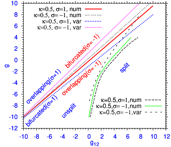
Figure 1: (Color online) Four curves on the left represent lines of the spontaneous symmetry breaking of symmetric ($\sigma=+1$) and antisymmetric ($\sigma=-1$) solitons, for $V_{0}=5$. Three curves on the right designate the onset of the spatial splitting between the components of symmetric and antisymmetric solitons. The results are obtained from the variational approximation (VA) and numerical simulations (num). Labels “overlapping/bifurcated” and “unsplit/split” indicate, respectively, areas of the existence of stable symmetric/asymmetric solitons, and of those with coinciding/separated centers of the two components.

The diagram covers both positive (repulsive) and negative (attractive) values of $g_{12}$ and $g$, the SSB line in quadrants $g_{12},g>0$ and $g_{12},g<0$ going, respectively, through families of GSs and regular solitons (the latter ones belong to the SIG). It is worthy to stress that the broken-symmetry areas are located on opposite sides of the SSB lines for $\sigma=+1$ and $-1$, i.e., for the the symmetric and antisymmetric solitons. The VA version of the splitting line for $\sigma=+1$ is not included in Fig. 1, as in this case SSB happens prior to the onset of the splitting, while Eq. (14) was derived from the VA assuming the unbroken symmetry. Note also that the SSB and splitting lines do not intersect, and there is no overlap between the stability areas of different types of the two-component solitons, i.e., the model does not give rise to a bistability.

The splitting lines displayed in Fig. 1 are similar to those reported in Ref. we for the model with $\kappa=0$ (nevertheless, the difference is that $\kappa\neq 0$ makes complete separation of the two components of the soliton impossible, unlike the situation with $\kappa=0$). On the other hand, all the results concerning the SSB lines have no previously published counterparts, as the symmetry breaking in regular and/or gap-mode solitons was not studied before in models featuring the competition between the linear coupling and nonlinear interaction between the species.

$\begin{array}[]{cc}\includegraphics[width=208.13574pt]{fig2a.eps}&\includegraphics[width=208.13574pt]{fig2b.eps}\\ \mathrm{(a)}&\mathrm{(b)}\\ \includegraphics[width=208.13574pt]{fig2c.eps}&\includegraphics[width=208.13574pt]{fig2d.eps}\\ \mathrm{(c)}&\mathrm{(d)}\\ \includegraphics[width=208.13574pt]{fig2e.eps}&\includegraphics[width=208.13574pt]{fig2f.eps}\\ \mathrm{(e)}&\mathrm{(f)}\end{array}$

Figure 2: (Color online) Examples of stable symmetric/asymmetric and unsplit/split solitons, as obtained from the numerical solution for different combinations of the attractive and repulsive interactions. The thin dashed curve depicts the OL potential, with $V_{0}=5$.

Figure 2 displays typical examples of SSB in symmetric and antisymmetric solitons [panels (a), (b) and (c), (d), respectively], and of the spatial splitting combined with SSB [(e), (f)]. To stress the role of the linear coupling in inducing the transition to the asymmetric shapes, the panels also include the case of $\kappa=0$. For all unsplit solitons, the shapes predicted by the VA, both symmetric and asymmetric ones, are virtually identical to the numerically found shapes shown in panels (a)-(d).

The case when the intra-species nonlinearity is switched off ($g=0$), and the solitons exist only due to the inter-species interactions, is of particular interest. The evolution of families of stable asymmetric GSs with the increase of $\left|g_{12}\right|$, as obtained from the numerical solution in this case (both for the attraction, $g_{12}<0$, and repulsion, $g_{12}>0$, when the solitons can be found, severally, only with $\sigma=-1$ or $\sigma=+1$), is shown in Fig. 3, for different values of linear coupling $\kappa$. In particular, the initial abrupt increase of $\epsilon$ with the growth of $g_{12}>0$ is the manifestation of the SSB in the unsplit GS. After achieving a maximum of $\epsilon$ very close to $1$, the asymmetric GS undergoes the splitting transition, which eventually leads to the gradual decrease of the effective asymmetry between the spatially separating components. In the case of $g_{12}<0$, the solitons (in this case, they belong to the SIG), also attain a maximum of $\epsilon$ very close to $1$. Further increase of $\left|g_{12}\right|$ leads to a transition to solitons of the symbiotic type symbiotic with reduced asymmetry. These results, as well as those summarized in Fig. 1, do not have previously published counterparts either.

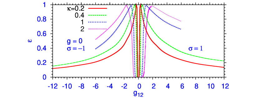
Figure 3: (Color online) The asymmetry of the solitons, $\epsilon$, defined as per Eq. (6), versus the nonlinear-coupling coefficient, $g_{12}$, as found from the numerical solution for $V_{0}=5,$ $g=0$, and $\sigma=1$ (four lines on the right side) or $\sigma=-1$ (four lines on the left side).

As mentioned above, the numerical procedure adopted in this work generates only stable soliton solutions. However, unlike the ordinary SIG-based solitons, GSs do not represent the BEC ground state GSprediction ; Markus , i.e., they are, strictly speaking, metastable objects. For this reason, it is relevant to test their stability against strong perturbations. Simulations demonstrate that the GSs are, in fact, very robust objects. For instance, sudden drop of the self-repulsion coefficient from $g=4$ to $g=1$, which can be easily implemented by means of FR, does not destroy the GS, see Fig. 4. Similarly, sudden application of a kick to the soliton (not shown here) gives rise to its oscillations around a local minimum of the OL potential, but does not destroy it either.

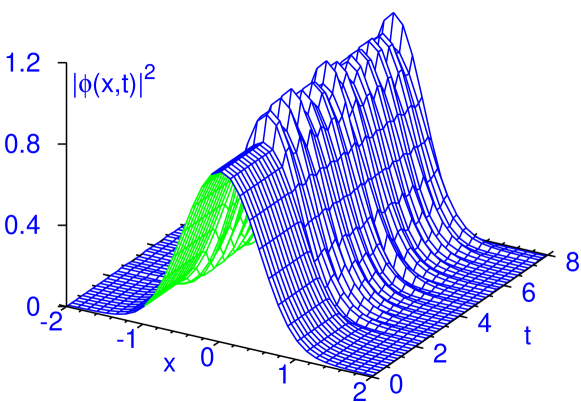
Figure 4: (Color online) The time evolution of the symmetric gap soliton found at $\sigma=1,$ $g=4,$ $g_{12}=2,$ $\kappa=0.2,$ $V_{0}=5$, after as $g$ suddenly dropped from $4$ to $1$. Here, $\phi_{1}=\phi_{2}\equiv\phi(x,t)$.

Conclusion. In this work, we have extended the model of binary BEC trapped in the OL potential we by including a the linear interconversion between the two species. Using the VA and numerical simulation, we have identified two internal transitions in two-component solitons, both regular and gap-mode ones: spontaneous symmetry breaking, and spatial splitting between the components.

This work was supported, in a part, by FAPESP and CNPq (Brazil).

References

- (1) K. E. Strecker et al., Nature 417, 150 (2002); L. Khaykovich et al., Science 256, 1290 (2002); S. L. Cornish, S. T. Thompson and C. E. Wieman, Phys. Rev. Lett. 96, 170401 (2006).
- (2) O. Zobay et al., Phys. Rev. A 59, 643 (1999); A. Trombettoni and A. Smerzi, Phys. Rev. Lett. 86, 2353 (2001); B. B. Baizakov, V. V. Konotop, and M. Salerno, J. Phys. B 35, 51015 (2002); P. J. Y. Louis et al., Phys. Rev. A 67, 013602 (2003).
- (3) B. Eiermann et al., Phys. Rev. Lett. 92, 230401 (2004).
- (4) C. J. Myatt et al.,Phys. Rev. Lett. 78, 586 (1997); D. M. Stamper-Kurn et al., Phys. Rev. Lett. 80, 2027 (1998).
- (5) A. Simoni et al. , Phys. Rev. Lett. 90, 163202 (2003).
- (6) V. M. Pérez-García and J. B. Beitia, Phys. Rev. A 72, 033620 (2005); S. K. Adhikari, Phys. Lett. A 346, 179 (2005); Phys. Rev. A 72, 053608 (2005); 70, 043617 (2004); 76, 053609 (2007); J. Phys. A 40, 2673 (2007).
- (7) A. Gubeskys, B. A. Malomed, and I. M. Merhasin, Phys. Rev. A 73, 023607 (2006).
- (8) M. Matuszewski, B. A. Malomed, and M. Trippenbach, Phys. Rev. A. 76, 043826 (2007).
- (9) S. K. Adhikari and B. A. Malomed, Phys. Rev. A 77, 023607 (2008).
- (10) R. J. Ballagh, K. Burnett, and T. F. Scott, Phys. Rev. Lett. 78, 1607 (1997).
- (11) J. Williams et al.,Phys. Rev. A 59, R31 (1999); P. Öhberg and S. Stenholm, Phys. Rev. A 59, 3890 (1999); D. T. Son and M. A. Stephanov, Phys. Rev. A 65, 063621 (2002); S. D. Jenkins and T. A. B. Kennedy, Phys. Rev. A 68, 053607 (2003).
- (12) M. I. Merhasin, B. A. Malomed, and R. Driben, J. Phys. B 38, 877(2005); S. K. Adhikari and B. A. Malomed, Phys. Rev. A 74, 053620 (2006).
- (13) A. Gubeskys and B. A. Malomed, Phys. Rev. A 75, 063602 (2007).
- (14) A. Gubeskys and B. A. Malomed, Phys. Rev. A 76, 043623 (2007); M. Matuszewski, B. A. Malomed, and M. Trippenbach, Phys. Rev. A 75, 063621 (2007); M. Trippenbach et al., Phys. Rev. A 78, 013603 (2008).
- (15) W. C. K. Mak, B. A. Malomed, and P. L. Chu, J. Opt. Soc. Am. B 15, 1685(1998); Phys. Rev. E 69, 066610 (2004); Y. J. Tsofe and B. A. Malomed, ibid. 75, 056603 (2007); S. Ha and A. A. Sukhorukov, J. Opt. Soc. Am. B 25, C15 (2008).
- (16) V. M. Pérez-García et al., Phys. Rev. A 56 1424 (1997); B. A. Malomed, Progress in Optics 43, 71 (2002).
- (17) A. Gubeskys, B. A. Malomed, and I. M. Merhasin, Stud. Appl. Math. 115, 255(2005).