Dipole model analysis of the newest diffractive deep inelastic scattering data

Abstract

We analyse the newest diffractive deep inelastic scattering data from the DESY collider HERA with the help of dipole models. We find good agreement with the data on the diffractive structure functions provided the diffractive open charm contribution is taken into account. However, the region of large diffractive mass (small values of a parameter $\beta$) needs some refinement with the help of an additional gluon radiation.

I Introduction

Diffractive deep inelastic scattering (DDIS), observed at the DESY collider HERA (see Aktas:2006hy ; Chekanov:2008cw and references therein) is one of the most intriguing phenomenons in the electron-proton $(ep)$ collisions. Despite high virtuality of the photonic probe, the incoming proton scatters intact being separated by a rapidity gap from a diffractive system, which is additionally formed in the final state. The understanding of these processes based on quantum chromodynamics (QCD) is the biggest challenge in the area of deep inelastic scattering. In this class of processes, large photon virtuality $Q^{2}$, which serves as a hard scale, suggests tha one use perturbative QCD with quarks and gluons as basic quanta. On the other hand, softness of the proton side and formation of the rapidity gap touch fundamental problems concerning transition into the nonperturbative domain of QCD. Thus, such important issues like parton saturation, unitarity and even confinement, are likely to be addressed in the theoretical description of diffractive processes.

The most promising QCD based approach to deep inelastic scattering (DIS) diffraction is formulated in terms of dipole models. In these models, the diffractive, color singlet state is systematically built from parton components of the light cone wave function of the virtual photon (see Wusthoff:1999cr ; Hebecker:1999ej and references therein). The lowest order states is formed by a quark-antiquark pair $(q\overline{q})$ while in higher orders more gluons $g$ and $q\overline{q}$ pairs are present. In our analysis we will concentrate on two first components, $q\overline{q}$ and $q\overline{q}g$, since in the configuration space they can be treated as simple, quark or gluon, color dipoles. Their interaction with the proton is described by the dipole scattering amplitude $N(x,r,b)$. Here $r$ and $b$ are two-dimensional vectors of transverse separation and impact parameter, respectively, and $x$ is the Bjorken variable which brings the energy dependence into the dipole models. The main advantage of this approach is the observation that the dipole scattering amplitude can be extracted from the DIS data on fully inclusive quantities, like the structure functions $F_{2}$ and $F_{L}$, based on some physically motivated form with a few parameters to fit Golec-Biernat:1998js ; Forshaw:1999uf ; Kowalski:2003hm ; Iancu:2003ge . Then, it can be used in the description of diffractive processes Golec-Biernat:1999qd ; Forshaw:1999ny ; Forshaw:2004xd ; Forshaw:2006np ; Marquet:2007nf ; Kowalski:2006hc . The form of $N$ which we use in our analysis is motivated by key features of parton saturation in dense partonic systems. The most important one is a saturation scale $Q_{s}(x)$ Golec-Biernat:1998js which can be extracted from the DIS data on the structure function $F_{2}$. The QCD based motivation for the existence of such a scale is provided by the analysis of the high energy nonlinear evolution equations of Balitsky and Kovchegov Balitsky:1995ub ; Kovchegov:1999yj ; Kovchegov:1999ua ; Kovchegov:1999ji .

In this analysis, we consider two important parameterisations of the dipole scattering amplitude, called Golec-Biernat-Wuesthoff (GBW) Golec-Biernat:1998js and color glass condensate (CGC) Soyez:2007kg , in which parton saturation results are built in. We present a precise comparison of the results of the dipole models which use these parameterisations with the newest data from HERA on the diffractive structure functions, obtained by the H1 Aktas:2006hy and ZEUS Chekanov:2008cw ; Chekanov:2008fh Collaborations. We also make a comparison with new data on the diffractive open charm production Aktas:2006up . An analysis of exclusive diffractive processes within the dipole approach was performed in Kowalski:2006hc . Previous analyses which use parton saturation results, like those in Golec-Biernat:1999qd ; Bartels:2002cj ; Goncalves:2004dv ; Kormilitzin:2007je ; Marquet:2007nf , are based on less precises diffractive data, and in consequence, they could not address important questions related the precise comparison presented in this paper.

The comparison we performed prompts us to discuss some subtle points of the dipole models, mostly related to the $q\overline{q}g$ component, and connect them to the approach based on the diffractive parton distributions evolved with the Dokshitzer-Gribov-Lipatov-Altarelli-Parisi (DGLAP) equations. Within the latter approach, the diffractive open charm production is particularly interesting since it is sensitive to a diffractive gluon distribution. However, the accuracy of the existing data on such a production does not allow one to discriminate between different gluon distributions considered in our analysis.

The outline of this presentation is the following. In Sec. II we present basic formulae of the color dipole approach to diffraction while in Sec. III we discuss the two parameterisations of the dipole scattering amplitude used in our analysis. In Sec. IV we perform a comparison of the dipole model results on the diffractive charm production with the HERA data. A similar comparison for the total diffractive structure functions is presented in Sec. V. In Appendix we derive a formula for the diffractive gluon distribution from dipole models, which is important for the discussion of the diffractive charm production.

II Diffractive structure functions in dipole models

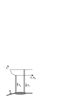
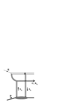
Figure 1: The $q\overline{q}$ i $q\overline{q}g$ components of the diffractive structure function $F_{2}^{D}$.

In the dipole approach to DDIS, the diffractive structure function $F_{2}^{D}$ is a sum of components corresponding to different diffractive final states produced by a transversely $(T)$ and longitudinally $(L)$ polarised virtual photon Bartels:1998ea . We consider a two component diffractive final state which is built from a $q\overline{q}$ pair from a transverse and longitudinal photon anda $q\overline{q}g$ system from a transverse photon, see Fig. 1. Thus, the structure function is given as a sum

$$F_{2}^{D}(x_{{I\!\!P}},\beta,Q^{2})=F_{T}^{(q\overline{q})}+F_{L}^{(q\overline{q})}+F_{T}^{(q\overline{q}g)}\,,$$ (1)

where the kinematic variables depend on diffractive mass $M$ and center-of-mass energy of the $\gamma^{*}p$ system $W$ through

$$x_{{I\!\!P}}=\frac{M^{2}+Q^{2}}{W^{2}+Q^{2}}\,,~{}~{}~{}~{}~{}~{}~{}~{}~{}~{}\beta=\frac{Q^{2}}{Q^{2}+M^{2}}$$ (2)

while the standard Bjorken variable $x=x_{{I\!\!P}}\beta$. The dependence of $F_{2}^{D}$ on the momentum transfer $t=(p-p^{\prime})^{2}$ is integrated out. The $q\overline{q}$ components from transversely and longitudinally polarised photons are given by

$$x_{{I\!\!P}}F_{T}^{(q\overline{q})}\!\! = \!\!\frac{3Q^{4}}{64\/\pi^{4}\beta B_{d}}\,\sum_{f}e_{f}^{2}\int_{z_{f}}^{1/2}dz\,z(1-z)$$ (3)

$$\times \left\{[z^{2}+(1-z)^{2}]\,Q^{2}_{f}\,\phi_{1}^{2}\,+\,m_{f}^{2}\,\phi_{0}^{2}\right\}~{}~{}~{}~{}~{}~{}~{}~{}$$

$$x_{{I\!\!P}}F_{L}^{(q\overline{q})}\!\! = \!\!\frac{3Q^{6}}{16\/\pi^{4}\beta B_{d}}\,\sum_{f}e_{f}^{2}\int_{z_{f}}^{1/2}dz\,z^{3}(1-z)^{3}\,\phi_{0}^{2}$$ (4)

where $f$ denotes quark flavours, $m_{f}$ is quark mass and the diffractive slope $B_{d}$ in the denominator results from the $t$-integration of the structure functions, assuming an exponential form for this dependence. From HERA data, $B_{d}=6~{}{\textrm{G}eV}^{-2}$. The variables

$$z_{f}={\textstyle{\frac{1}{2}}}(1-\sqrt{1-4m_{f}^{2}/M^{2}})\,,~{}~{}~{}~{}Q^{2}_{f}=z(1-z)Q^{2}+m_{f}^{2}$$ (5)

and the functions $\phi_{i}$ take the following form for $i=0,1$

$$\phi_{i}=\int_{0}^{\infty}drrK_{i}\!\left(Q_{f}r\right)J_{i}\!\left(k_{f}r\right)\hat{\sigma}(x_{{I\!\!P}},r)$$ (6)

where $k_{f}=\sqrt{z(1-z)M^{2}-m_{f}^{2}}$ is the quark transverse momentum while $K_{i}$ and $J_{i}$ are the Bessel functions. The lower integration limit $z_{f}$ in Eqs. (3) and (4) corresponds to a minimal value of $z$ for which the diffractive state with mass $M$ can be produced. In such a case $k_{f}=0$. At the threshold for the massive quark production $M^{2}=4m_{f}^{2}$ and $z_{f}=1/2$, leading to $F_{T,L}^{(q\overline{q})}=0$. For massless quarks $z_{f}=0$.

The quantity $\hat{\sigma}(x_{{I\!\!P}},r)$ in Eq. (6) is called a dipole cross section and described the interaction of the $q\overline{q}$ dipole with the proton. It brings the energy dependence into the structure function formulae and is related to the imaginary part of the dipole scattering amplitude, $N(x_{{I\!\!P}},r,b)$, by the integral over the impact parameter

$$\hat{\sigma}(x_{{I\!\!P}},r)=2\int d^{2}b\,N(x_{{I\!\!P}},r,b)\,.$$ (7)

Notice that for DDIS the Bjorken variable $x$ is substituted by $x_{{I\!\!P}}=x/\beta$. For $\beta\sim 1$ this substitution is subleading from the point of view leading logarithms of energy $W$ which appear in the QCD computation of this amplitude. However, for large diffractive masses, $\beta\ll 1$, such a substitution becomes phenomenologically important.

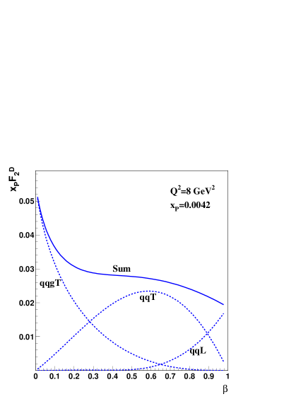
Figure 2: The three components in Eq. (1) as a function of $\beta$ in the massless quark limit with the GBW parameterisation of the dipole cross section. The $q\overline{q}gT$ component is without the color factor modification.

The $q\overline{q}g$ diffractive component from transverse photons, computed for massless quarks is given by

$$x_{{I\!\!P}}F_{T}^{(q\overline{q}g)} = \frac{81\beta\alpha_{s}}{512\pi^{5}B_{d}}\;\sum_{f}e_{f}^{2}\int_{\beta}^{1}\frac{dz}{(1-z)^{3}}$$ (8)

$$\times \left[\left(1-\frac{\beta}{z}\right)^{2}+\left(\frac{\beta}{z}\right)^{2}\right]$$

$$\times \int_{0}^{(1-z)Q^{2}}dk^{2}\log\left(\frac{(1-z)Q^{2}}{k^{2}}\right)\phi_{2}^{2}$$

where the function $\phi_{2}$ takes to form

$$\phi_{2}=k^{2}\int_{0}^{\infty}dr\,r\,K_{2}\!\left(\sqrt{\frac{z}{1-z}}kr\right)\,J_{2}(kr)\,\hat{\sigma}(x_{{I\!\!P}},r)$$ (9)

with $K_{2}$ and $J_{2}$ are the Bessel functions. In papers Wusthoff:1997fz ; Golec-Biernat:1999qd , formula (8) was computed with two gluons exchanged between the diffractive system and the proton. Then, the two gluon exchange interaction was substituted by the dipole cross section $\hat{\sigma}=\hat{\sigma}(x_{{I\!\!P}},r)$ for the $q\overline{q}$ dipole interaction with the proton. For example, for the GBW parameterisation of the dipole cross section Wusthoff:1997fz , which we discuss in the next section, is given by

$$\hat{\sigma}\equiv\hat{\sigma}_{q\overline{q}}=\sigma_{0}\left(1-{\mbox{{e}}}^{-r^{2}Q_{s}^{2}/4}\right)\,.$$ (10)

However, the $q\overline{q}g$ system was computed in the approximation when parton transverse momenta fulfil the condition $k_{Tq}\approx k_{T\overline{q}}\gg k_{Tg}$. Thus, in the large $N_{c}$ approximation, it can be treated as a gluonic color dipole $gg$. Such a dipole interacts with the relative color factor $C_{A}/C_{F}$ with respect to the $q\overline{q}$ dipole. Therefore, the two gluon exchange formula should be eikonalized with this color factor absorbed into the exponent. For the GBW parameterisation, this leads to the following gluon dipole cross section in Eq. (9)

$$\hat{\sigma}\equiv\hat{\sigma}_{gg}=\sigma_{0}\left(1-{\mbox{{e}}}^{-(C_{A}/C_{F})r^{2}Q_{s}^{2}/4}\right)\,.$$ (11)

In such a case, the color factor $C_{A}/C_{F}=9/4$ (for $N_{c}=3$) disappears from the normalisation of the scattering amplitude and we have to rescale the structure function in the following way

$$F_{T}^{(q\overline{q}g)}~{}\to~{}\frac{1}{(C_{A}/C_{F})^{2}}\,F_{T}^{(q\overline{q}g)}\,.$$ (12)

By the comparison with HERA data, we will show in the next section that the latter possibility is more appropriate for the data description.

We summarise our considerations in Fig. 2, which shows three components of $F_{2}^{D}$ as a function of $\beta$ for fixed values of $x_{{I\!\!P}}$ and $Q^{2}$. Each component dominates in different regions of diffractive mass: $F_{T}^{(q\overline{q})}$ dominates for $M^{2}\sim Q^{2}$ ($\beta\sim 1/2$), $F_{L}^{(q\overline{q})}$ is important for $M^{2}\ll Q^{2}$ ($\beta\approx 1$) and $F_{T}^{(q\overline{q}g)}$ wins for large diffractive mass, $M^{2}\gg Q^{2}$ ($\beta\ll 1$).

III Dipole scattering amplitude

We are going to compare the presented dipole description of the diffractive structure functions with the newest HERA data. For this purpose, we consider two parameterisations of the dipole cross section which are based on the idea of parton saturation in dense gluon systems. The first one is the GBW parameterisation with heavy quarks Golec-Biernat:1998js which has played an inspirational role in studies of parton saturation in the recent ten years. The second one is the CGC parameterisation Iancu:2003ge ; Soyez:2007kg which somehow summarizes the studies within the Color Glass Condensate Iancu:2003xm approach to parton saturation. Quite surprisingly, these two parameterisations give very similar results for the diffractive structure functions. The main reason is the same normalisation of the dipole cross section, $\sigma_{0}$. The origin of the same numerical value, however, is different. For the GBW parameterisation $\sigma_{0}$ is fitted to the data for $F_{2}$ while for the CGC parameterisation it is computed from a diffractive slope $B_{D}$, see Eq. (18).

The two considered parameterisations, specified below, describe very well the inclusive DIS data on the structure function $F_{2}$. Their use for the DDIS description is a very important test of the universality of the dipole approach to DIS diffraction.

• it The GBW parameterisation with heavy quarks has the following form of the $q\overline{q}$ dipole cross section Golec-Biernat:1998js

  $$\hat{\sigma}(x_{{I\!\!P}},r)=\sigma_{0}\left(1-\exp(-r^{2}Q_{s}^{2}/4\right))$$ (13)

  where $\sigma_{0}=29~{}{\textrm{m}b}$, and the saturation scale is given by

  $$Q_{s}^{2}=\left({x_{{I\!\!P}}}/{x_{0}}\right)^{-\lambda}~{}{\textrm{G}eV}^{2}$$ (14)

  with $x_{0}=4\cdot 10^{-5}$ and $\lambda=0.288$. The dipole scattering amplitude in such a case reads

  $$\hat{N}(x_{{I\!\!P}},{\bf r},{\bf b})=\theta(b_{0}-b)\left(1-\exp(-r^{2}Q_{s}^{2}/4\right)$$ (15)

  where $2\pi b_{0}^{2}=\sigma_{0}$. This form corresponds to a model of the proton with a sharp edge.

• The CGC parameterisation with heavy quarks of the quark dipole scattering amplitude is given by Iancu:2003ge ; Soyez:2007kg ; Marquet:2007nf

  $$\hat{N}(x_{{I\!\!P}},{\bf r},{\bf b})=S({\bf b})\,N(x_{{I\!\!P}},{\bf r})\,.$$ (16)

  where the form factor $S({\bf b})=\exp(-b^{2}/(2B_{d}))$ with the diffractive slope from HERA, $B_{d}=6~{}{\textrm{G}eV}^{-2}$. Thus, the dipole cross section (7) is given by the formula

  $$\hat{\sigma}(x_{{I\!\!P}},{\bf r})=4\pi B_{d}\,N(x_{{I\!\!P}},{\bf r})\,.$$ (17)

  We see that the asymptotic value of $\hat{\sigma}$ for $r\to\infty$ is the same as for the GBW parameterisation, if the diffractive slope measured at HERA is substituted,

  $$\sigma_{0}=4\pi B_{d}=29~{}{\textrm{m}b}\,.$$ (18)

  In addition,

  $$N(x_{{I\!\!P}},{\bf r})=$$ (19)

  $$\left\{\begin{array}[]{ll}N_{0}\left(\frac{rQ_{s}}{2}\right)^{2\gamma_{s}}{\mbox{{e}}}^{\frac{2\ln^{2}(rQ_{s}/2)}{\kappa\lambda\ln(x_{{I\!\!P}})}}&\mbox{{f}or~{}~{}~{} $rQ_{s}\leq 2$}\\ 1-{\mbox{{e}}}^{-4\alpha\ln^{2}(\beta rQ_{s})}&\mbox{{f}or~{}~{}~{} $rQ_{s}>2$}\end{array}\right.$$ (22)

  where the saturation scale $Q_{s}$ has now the following parameters: $\lambda=0.22$ and $x_{0}=1.63\cdot 10^{-5}$. The parameters $\alpha=0.615$ and $\beta=1.006$ are chosen such that $N$ and its first derivative are continues at the point $r$ where $N(r)=N_{0}=0.7$. The remaining parameters are given by $\kappa=9.9$ and $\gamma_{c}=0.7376$.

Both parameterisations provide the energy dependence of the diffractive structure function through the variable $x_{{I\!\!P}}$. This dependence is determined from fits of the dipole model formula for $F_{2}$ into the data from HERA for the Bjorken variable $x\leq 0.01$. In the case of DDIS, $x$ is substituted by $x_{{I\!\!P}}$.

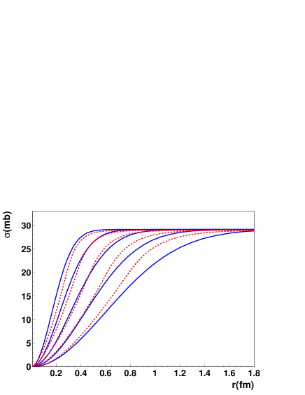
Figure 3: The dipole cross section as a function of $r$ for $x=10^{-2}\ldots 10^{-6}$ (from right to left) and for the GBW (continuous lines) and CGC (dashed lines) parameterisations.

IV Diffractive charm quark production

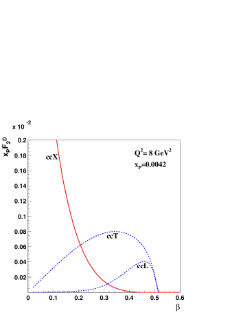
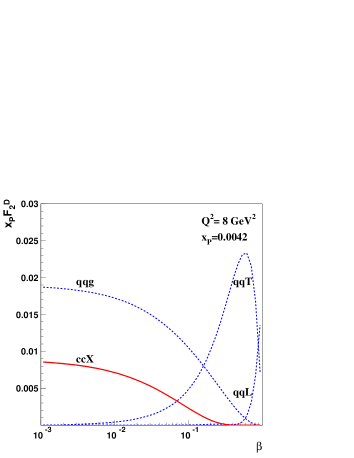
Figure 4: Top: the $c\overline{c}T$ and $c\overline{c}L$ components of $F_{2}^{D}$ from the dipole model with the GBW parameterisation together with the $c\overline{c}X$ contribution from the collinear factorisation approach (26) with the diffractive gluon distribution (38). Bottom: the $c\overline{c}X$ component in a different scale against the massless $q\overline{q}T$, $q\overline{q}L$ and $q\overline{q}g$ components.

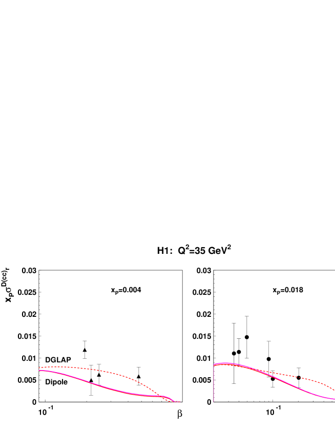
Figure 5: A comparison of the collinear factorisation predictions with the GBW and CGC gluon distributions (solid lines) with the HERA data on the open diffractive charm production. The dashed lines are computed with the gluon distribution obtained in the DGLAP fit GolecBiernat:2007kv to the H1 data on the diffractive structure functions.

In the diffractive scattering heavy quarks are produced in quark-antiquark pairs, $c\overline{c}$ and $b\overline{b}$ for charm and bottom, respectively. Such pairs can be produced provided that the diffractive mass of is above the quark pair production threshold

$$M^{2}=Q^{2}\left(\frac{1}{\beta}-1\right)>4m_{c,b}^{2}$$ (23)

In the lowest order the diffractive state consist only the $c\overline{c}$ or $b\overline{b}$ pair. In the forthcoming we consider only charm production since bottom production is negligible. The corresponding contributions to $F_{2}^{D}$ are given by Eqs. (3) and (4) with one flavour component. For example, for charm production from transverse photons we have

$$x_{{I\!\!P}}F_{T}^{(c\overline{c})}\!\! = \!\!\frac{3Q^{4}e_{c}^{2}}{64\/\pi^{4}\beta B_{d}}\int_{z_{c}}^{1/2}dz\,z(1-z)$$ (24)

$$\times \left\{[z^{2}+(1-z)^{2}]\,Q^{2}_{c}\,\phi_{1}^{2}\,+\,m_{c}^{2}\,\phi_{0}^{2}\right\}$$

where $m_{c}$ and $e_{c}$ are charm quark mass and electric charge, respectively. The minimal value of diffractive mass equals $M^{2}_{min}=4m_{c}^{2}$, thus the maximal value of $\beta$ is given by

$$\beta_{max}=\frac{Q^{2}}{Q^{2}+4m_{c}^{2}}\,.$$ (25)

In such a case, $z_{c}=1/2$ in Eq. (24) and $F_{T,L}^{(c\overline{c})}=0$ for $\beta>\beta_{max}$. This is shown in Fig. 4 (top) for the $c\overline{c}$ diffractive states from transverse $(c\overline{c}T)$ and longitudinal $(c\overline{c}L)$ photons. By the comparison with the corresponding curves for three massless quarks $(q\overline{q}T,q\overline{q}L)$, shown in Fig. 4 (bottom), we see that the exclusive diffractive charm production contributes only $1/30$ to the total structure function $F_{2}^{D}$. Thus it can practically be neglected.

The next component is the $c\overline{c}g$ diffractive state. Unfortunately, formula (8) for the $q\overline{q}g$ production is only known in the massless quark case and cannot be used for heavy quarks. Thus, we have to resort to the collinear factorisation formula, given by Eq. (26), in which the charm-anticharm pair is produced via the photon-gluon fusion: $\gamma^{*}g\to c\overline{c}$ Goncalves:2004dv . If such an approach is applied to diffractive scattering, gluon is a “constituent of a pomeron”. The diffractive state consists of additional particles $X$ (called “pomeron remnant”) in addition to the heavy quark pair, which is well separated in rapidity from the scattered proton. The collinear factorisation formula for the charm contribution to the diffractive structure functions is taken from the fully inclusive case Gluck:1994uf in which the standard gluon distribution is replaced by the diffractive gluon distribution $g^{D}$:

$$x_{{I\!\!P}}F_{2,L}^{D(c\overline{c}X)}\!\! = \!\!2\beta\,e_{c}^{2}\,\frac{\alpha_{s}(\mu_{c}^{2})}{2\pi}\int_{a\beta}^{1}\frac{dz}{z}\,C_{2,L}\!\left(\frac{\beta}{z},{\frac{m_{c}^{2}}{Q^{2}}}\right)$$ (26)

$$\times x_{{I\!\!P}}g^{D}(x_{{I\!\!P}},z,\mu_{c}^{2})$$

where $a=1+4m_{c}^{2}/Q^{2}$ and the factorisation scale $\mu_{c}^{2}=4m_{c}^{2}$ with the charm quark mass $m_{c}=1.4~{}{\textrm{G}eV}$. The leading order coefficient functions are given by

$$C_{2}(z,r)\!\! = \!\!\textstyle{\frac{1}{2}}\left\{z^{2}+(1-z)^{2}+4z(1-3z)r-8z^{2}r^{2}\right\}$$ (27)

$$\times \ln{\frac{1+\alpha}{1-\alpha}}\,+\,\textstyle{\frac{1}{2}}\alpha\big{\{}-1+8z(1-z)$$

$$- 4z(1-z)r\big{\}}$$

$$C_{L}(z,r)\!\! = \!\!-4z^{2}r\ln{{1+\alpha}{1-\alpha}}+2\alpha z(1-z)$$ (28)

where $r={m_{c}^{2}}/{Q^{2}}$ and $\alpha=\sqrt{1-{4rz}/{(1-z)}}$. The lower integration limit in Eq. (26) results from the condition for the heavy quark production in the fusion: $\gamma^{*}g\to c\overline{c}$,

$$(zx_{{I\!\!P}}\,p+q)^{2}\geq 4m_{c}^{2}$$ (29)

where we assume that gluon carries a fraction $z$ of the pomeron momentum $x_{{I\!\!P}}p$.

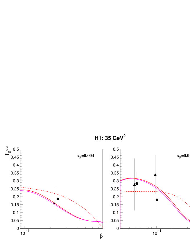
Figure 6: The fractional charm contribution, $f_{D}^{c\overline{c}}$ given by Eq. (31), is shown as a function of $\beta$, for two values of $x_{{I\!\!P}}=0.004$ and $0.018$. The solid lines are computed for the $c\overline{c}X$ contribution with the GBW and CGC diffractive gluon distributions while the dashed lines are found for the diffractive gluon distribution obtained in the DGLAP fit GolecBiernat:2007kv to the H1 Collaboration data.

The $c\overline{c}X$ contribution given by Eq. (26) is shown in Fig. 4 as the solid lines. As seen in the top figure, this component becomes significant for $\beta<0.1$ . By a comparison with the massless quark contributions (the bottom figure) we see that diffractive charm production contributes up to $30\%$ to the diffractive structure function $F_{2}^{D}$ for small values of $\beta$. The presented results were obtained assuming the diffractive gluon distribution which results from the dipole models, given by Eq. (38) in Appendix, with the GBW parameterisation of the dipole cross section with the color factor modification (40). The CGC parameterisation gives a similar result.

In Fig. 5 we show the collinear factorisation predictions for the diffractive charm production confronted with the new HERA data Aktas:2006up on the charm component of the reduced cross section:

$$\sigma_{r}^{D(c\overline{c})}=F_{2}^{D(c\overline{c})}-\frac{y^{2}}{1+(1-y)^{2}}F_{L}^{D(c\overline{c})}\,.$$ (30)

The solid curves, which are barley distinguishable, correspond to the result with the GBW and CGC parameterisations of the diffractive gluon distributions. The dashed lines are computed for the gluon distribution from a fit to the H1 data GolecBiernat:2007kv based on the DGLAP equations. The present accuracy of the charm data does not allow to discriminate between these two approaches although the data seem to prefer the gluon distribution from the DGLAP fit which is much more concentrated in the large $z$-region as compared to the dipole model gluon distributions, see Fig. 11 in Appendix.

The importance of diffractive charm is illustrated in Fig. 6 where the fractional charm contribution,

$$f_{D}^{c\overline{c}}={\sigma_{r}^{D(c\overline{c})}}/{\sigma_{r}^{D}}\,,$$ (31)

to the total diffractive cross section, discussed in the next section, is shown as a function of $\beta$ against the H1 Collaboration data Aktas:2006up . For small values of $\beta$, the charm contribution equals on average approximately $20-30\%$, which is comparable to the charm fraction in the inclusive cross section for similar values of $Q^{2}$ Aktas:2005iw .

V Comparison with the HERA data

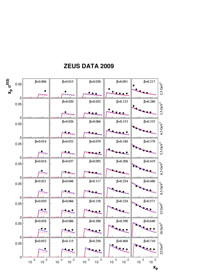
Figure 7: A comparison of $\sigma_{r}^{D}$ from the two considered dipole models with the newest ZEUS Collaboration data Chekanov:2008fh . The solid lines correspond to the GBW parameterisation of the dipole cross section with the color factor modifications (11) and (12), while the dotted lines correspond to the CGC parameterisation. The dashed lines show the results without the charm contribution.

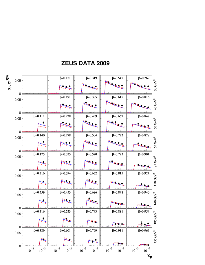
Figure 8: The same as in Fig. 7 but for higher values of $Q^{2}$. The dashed lines show the contribution without charm.

In Figs. 7 and 8 we show a comparison of the dipole model predictions with the ZEUS Collaboration data Chekanov:2008fh on the reduced cross section

$$\sigma_{r}^{D}=F_{2}^{D}-\frac{y^{2}}{1+(1-y)^{2}}F_{L}^{D}\,.$$ (32)

We included the charm contribution in the above structure functions. The solid lines correspond to the GBW parameterisation of the dipole cross section with the color factor modifications (11) and (12) of the $q\overline{q}g$ component, while the dashed lines are obtained from the CGC parameterisation. We see that the two sets of curves are barely distinguishable. This somewhat surprising results could be attributed to the same normalisation of the dipole cross section in both models, $\sigma_{0}=29~{}{\rm mb}$. Let us emphasise again that this numerical value was obtained in two different ways (see Sec. III for more details). The color factor modification of the $q\overline{q}g$ component in the GBW parameterisation is necessary since the curves without such a modification significantly overshoot the data (by a factor of two or so) in the region of small $\beta$ where the ${q\overline{q}g}$ component dominates.

The comparison of the predictions with the data also reveals a very important aspect of the three component dipole model (1). In the small $\beta$ region, the curves are systematically below the data points, which effect may be attributed to the lack of higher order components in the diffractive state, i.e. with more than one gluon or $q\overline{q}$ pair. This is also seen for the H1 Collaboration data Aktas:2006hy shown in Fig. 9. For small values of $\beta$ both the solid (GBW) and dashed (CGC) curves are below the data. It is also important that the charm contribution, described in Sec. IV, is added into the analysis. Without this contribution the comparison would be much worse than that shown here.

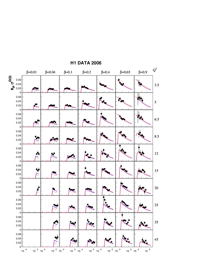
Figure 9: The same as in Fig. 7 but for the H1 Collaboration data Aktas:2006hy . The dashed lines show the contribution without charm.

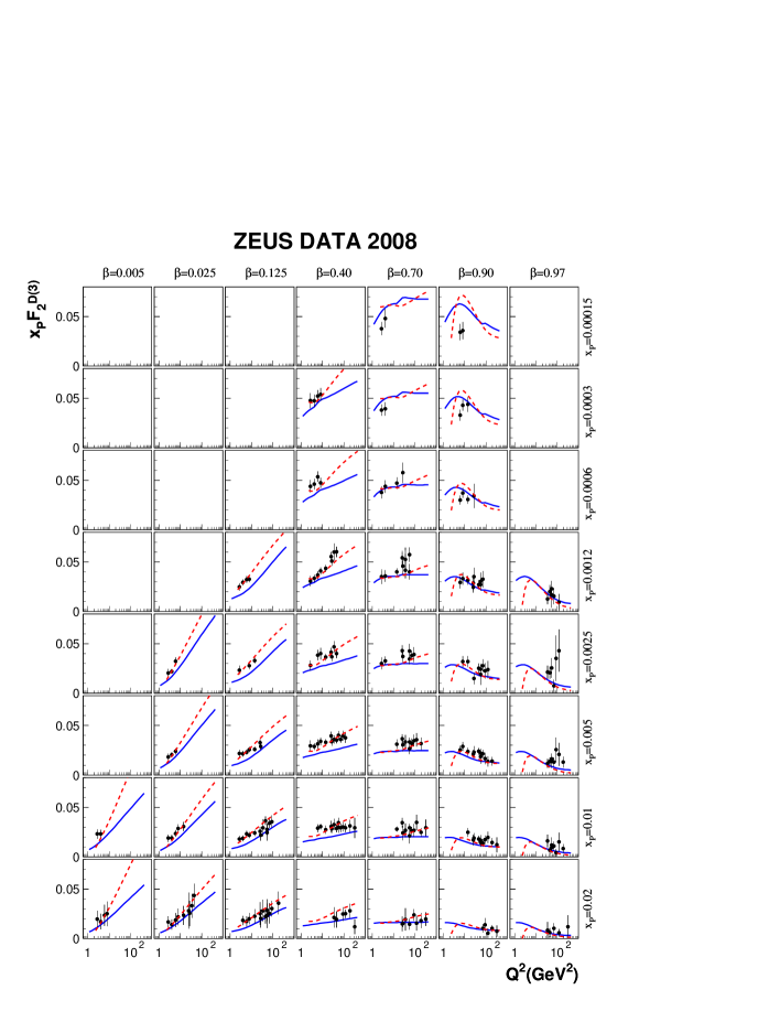
Figure 10: A comparison of the GBW dipole model predictions (solid lines) and the results from the DGLAP fit (dashed lines) GolecBiernat:2007kv to the ZEUS data Chekanov:2008cw .

This effect may be attributed to the lack of higher order components in the diffractive state, i.e. with more than one gluon or $q\overline{q}$ pair. They may be added in the DGLAP based approach to inclusive diffraction which sums additional partonic emissions in the diffractive state in the transverse momentum ordering approximation. A comprehensive discussion of the DGLAP based fits to the diffractive HERA data is presented in GolecBiernat:2007kv . We only recall here that in this approach the diffractive structure functions are twist-$2$ quantities with the logarithmic dependence on $Q^{2}$ for fixed $x_{{I\!\!P}}$ and $\beta$. They are related to the diffractive parton distributions by the standard collinear factorisation formulae, e.g. in the leading $\log Q^{2}$ approximation we have:

$$F_{2}^{D}(x_{{I\!\!P}},\beta,Q^{2})=\sum_{f}e_{f}^{2}\,\beta\,(q^{D}_{f}+\overline{q}^{D}_{f})\,,$$ (33)

where $q_{f}^{D}$ and $\overline{q}^{D}_{f}$ are diffractive quark/antiquark distributions. We additionally assume flavour democracy for these distributions to account for vacuum quantum number exchange responsible for diffraction,

$$q^{D}_{f}=\overline{q}^{D}_{f}=\frac{1}{2N_{f}}\Sigma^{D}$$ (34)

where $\Sigma^{D}$ is a diffractive singlet quark distribution. This distribution is evolved in $Q^{2}$ by the DGLAP equations together with the gluon distribution $g^{D}$. In contrast to the dipole model case, the $x_{{I\!\!P}}$ dependence of the diffractive parton distributions is fitted to data, as well as their form in $\beta$ at some initial scale $Q_{0}^{2}$. In Fig. 10 we show the result of such an analysis (dashed lines) applied to the ZEUS data Chekanov:2008cw . In the small$-\beta$ region, the DGLAP fit curves are going through the experimental points with larger logarithmic slope, $\partial F_{2}^{D}/\partial\ln Q^{2}$, than in the dipole approach. This illustrates the importance of more complicated diffractive states than the $q\overline{q}g$ state.

VI Conclusions

We presented a comparison of the dipole model results on the diffractive structure functions with the HERA data. We considered two most popular parameterisations of the interaction between the diffractive system and the proton (the GBW and CGC parameterisations) which are based on the idea of parton saturation. The three component model with the $q\overline{q}$ and $q\overline{q}g$ diffractive states describe reasonable well the recent data. However, the region of small values of $\beta$ needs some refinement by considering components with more gluons and $q\overline{q}$ pairs in the diffractive state. This can be achieved in the DGLAP based approach which sums partonic emissions in the diffractive state in the transverse momentum ordering approximation. We extracted the diffractive gluon distribution from the dipole model formulae to use it for the computation of the charm contribution to $F_{2}^{D}$. We found good agreement with the HERA data on the diffractive open charm production both for the the gluon distributions from the considered dipole models and the DGLAP fits from GolecBiernat:2007kv . The latter statement, however, is possible to make only due to present accuracy of the charm data. The results presented in this work might be a starting point for the future electron-proton collider LHeC at CERN.

*

Appendix A Diffractive gluon distribution from dipole models

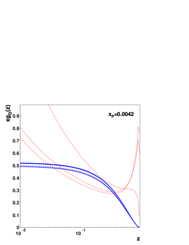
Figure 11: The diffractive gluon distribution $xg_{D}(x_{{I\!\!P}},z,Q^{2})$ for $Q^{2}=4m_{c}^{2},\,7.84,\,10,\,100~{}\mbox{GeV}^{2}$ (from bottom to top) and $x_{{I\!\!P}}=0.0042$. The solid lines correspond to the GBW parameterisation while the dashed lines to the CGC parameterisation. The dotted lines show the gluon distributions from the DGLAP fit GolecBiernat:2007kv to the H1 Collaboration data.

A comprehensive discussion of the derivation of the diffractive parton distributions in dipole models can be found in Golec-Biernat:2001mm . Here we only recall the derivation of the diffractive gluon distribution $g^{D}(x_{{I\!\!P}},z,Q^{2})$ which supplements that in Golec-Biernat:2001mm . We start from Eq. (8) which we reduce to the collinear factorisation form. Let us substitute $(1-z)Q^{2}\to Q^{2}$ in there. We numerically checked that such a substitution practically does not change the diffractive structure function. Then the logarithmic derivative of $F_{T}^{(q\overline{q}g)}$ reads

$$\frac{\partial F_{T}^{(q\overline{q}g)}}{\partial\ln Q^{2}}\!\! = \!\!\frac{81\beta\alpha_{s}}{512\pi^{5}x_{{I\!\!P}}B_{d}}\,\sum_{f}e_{f}^{2}\int_{\beta}^{1}\frac{dz}{z}\left[\left(1-\frac{\beta}{z}\right)^{2}+\right.$$ (35)

$$+ \left.\left(\frac{\beta}{z}\right)^{2}\right]\frac{z}{(1-z)^{3}}\int_{0}^{Q^{2}}dk^{2}\phi_{2}^{2}\,.$$

On the other hand, from the DGLAP evolution equation we have for the diffractive singlet quark distribution (34)

$$\frac{\partial\Sigma^{D}}{\partial\ln Q^{2}}\!\! \approx \!\!\frac{\alpha_{s}(Q^{2})}{2\pi}\int_{\beta}^{1}\frac{dz}{z}\,N_{f}\left\{\left(1-\frac{\beta}{z}\right)^{2}+\left(\frac{\beta}{z}\right)^{2}\right\}$$ (36)

$$\times g^{D}(x_{{I\!\!P}},z,Q^{2})$$

where we neglected on the right hand side a contribution with the singlet quark distribution which is much smaller than the gluonic one when $\beta\ll 1$. Thus from Eq. (33) we find for the diffractive structure function

$$\frac{\partial F_{2}^{D}}{\partial\ln Q^{2}}\!\! = \!\!\frac{\beta\alpha_{s}}{2\pi}\,\sum_{f}e_{f}^{2}\int_{\beta}^{1}\frac{dz}{z}\left\{\left(1-\frac{\beta}{z}\right)^{2}+\left(\frac{\beta}{z}\right)^{2}\right\}$$ (37)

$$\times g^{D}(x_{{I\!\!P}},z,Q^{2})\,.$$

For small $\beta$ we have: $F_{T}^{(q\overline{q}g)}\approx F_{2}^{D}$, thus by the comparison with Eq. (35), we find the following diffractive gluon distribution

$$g^{D}(x_{{I\!\!P}},z,Q^{2})=\frac{81}{256\pi^{4}x_{{I\!\!P}}B_{d}}\frac{z}{(1-z)^{3}}\int_{0}^{Q^{2}}dk^{2}\,\phi_{2}^{2}$$ (38)

where

$$\phi_{2}=k^{2}\int_{0}^{\infty}dr\,r\,K_{2}\!\left(\sqrt{{z}/{(1-z)}}kr\right)\,J_{2}(kr)\,\hat{\sigma}(x_{{I\!\!P}},r)\,.$$ (39)

For the GBW parameterisation of the dipole cross section, we additionally rescale the gluon distribution,

$$g^{D}~{}\to~{}\frac{1}{(C_{A}/C_{F})^{2}}\,\,g^{D}\,,$$ (40)

and use formula (11) for the dipole cross section. For the CGC parameterisation this rescaling has been already taken into account. In Fig. 11 we show the gluon distributions computed for the GBW parameterisation with the color factor modification (solid lines) and for the CGC parameterisation (dashed lines). There is practically no difference between them for the indicated scales. For $Q^{2}>4m_{c}^{2}$, the $Q^{2}$ dependence of the gluon distribution (38) is already very weak and close to the asymptotic limit obtained for $Q^{2}\to\infty$. We also show in this figure the gluon distributions found in a DGLAP fit with higher twist to the recent H1 data GolecBiernat:2007kv (dotted lines) with a strong dependence on $Q^{2}$ due to the DGLAP evolution.

References

- (1) H1, A. Aktas et al., Eur. Phys. J. C48, 715 (2006), [hep-ex/0606004].
- (2) ZEUS, S. Chekanov et al., Nucl. Phys. B800, 1 (2008), [0802.3017].
- (3) M. Wusthoff and A. D. Martin, J. Phys. G25, R309 (1999), [hep-ph/9909362].
- (4) A. Hebecker, Phys. Rept. 331, 1 (2000), [hep-ph/9905226].
- (5) K. Golec-Biernat and M. Wusthoff, Phys. Rev. D59, 014017 (1999), [hep-ph/9807513].
- (6) J. R. Forshaw, G. Kerley and G. Shaw, Phys. Rev. D60, 074012 (1999), [hep-ph/9903341].
- (7) H. Kowalski and D. Teaney, Phys. Rev. D68, 114005 (2003), [hep-ph/0304189].
- (8) E. Iancu, K. Itakura and S. Munier, Phys. Lett. B590, 199 (2004), [hep-ph/0310338].
- (9) K. Golec-Biernat and M. Wusthoff, Phys. Rev. D60, 114023 (1999), [hep-ph/9903358].
- (10) J. R. Forshaw, G. R. Kerley and G. Shaw, Nucl. Phys. A675, 80c (2000), [hep-ph/9910251].
- (11) J. R. Forshaw, R. Sandapen and G. Shaw, Phys. Lett. B594, 283 (2004), [hep-ph/0404192].
- (12) J. R. Forshaw, R. Sandapen and G. Shaw, JHEP 11, 025 (2006), [hep-ph/0608161].
- (13) C. Marquet, Phys. Rev. D76, 094017 (2007), [0706.2682].
- (14) H. Kowalski, L. Motyka and G. Watt, Phys. Rev. D74, 074016 (2006), [hep-ph/0606272].
- (15) I. Balitsky, Nucl. Phys. B463, 99 (1996), [hep-ph/9509348].
- (16) Y. V. Kovchegov, Phys. Rev. D60, 034008 (1999), [hep-ph/9901281].
- (17) Y. V. Kovchegov, Phys. Rev. D61, 074018 (2000), [hep-ph/9905214].
- (18) Y. V. Kovchegov and E. Levin, Nucl. Phys. B577, 221 (2000), [hep-ph/9911523].
- (19) G. Soyez, Phys. Lett. B655, 32 (2007), [0705.3672].
- (20) ZEUS, S. Chekanov et al., 0812.2003.
- (21) H1, A. Aktas et al., Eur. Phys. J. C50, 1 (2007), [hep-ex/0610076].
- (22) J. Bartels, K. Golec-Biernat and H. Kowalski, Phys. Rev. D66, 014001 (2002), [hep-ph/0203258].
- (23) V. P. Goncalves and M. V. T. Machado, Phys. Lett. B588, 180 (2004), [hep-ph/0401104].
- (24) A. Kormilitzin, 0707.2202.
- (25) J. Bartels, J. R. Ellis, H. Kowalski and M. Wusthoff, Eur. Phys. J. C7, 443 (1999), [hep-ph/9803497].
- (26) M. Wusthoff, Phys. Rev. D56, 4311 (1997), [hep-ph/9702201].
- (27) E. Iancu and R. Venugopalan, hep-ph/0303204.
- (28) K. J. Golec-Biernat and A. Luszczak, Phys. Rev. D76, 114014 (2007), [0704.1608].
- (29) M. Gluck, E. Reya and A. Vogt, Z. Phys. C67, 433 (1995).
- (30) H1, A. Aktas et al., Eur. Phys. J. C45, 23 (2006), [hep-ex/0507081].
- (31) K. Golec-Biernat and M. Wusthoff, Eur. Phys. J. C20, 313 (2001), [hep-ph/0102093].