Rings, spirals and manifolds

Abstract

Two-armed, grand design spirals and inner and outer rings in barred galaxies can be due to orbits guided by the manifolds emanating from the vicinity of the $L_{1}$ and $L_{2}$ Lagrangian points, located at the ends of the bar. We first summarise the necessary theoretical background and in particular we describe the dynamics around the unstable equilibrium points in barred galaxy models, and the corresponding homoclinic and heteroclinic orbits. We then discuss two specific morphologies and the circulation of material within the corresponding manifolds. We also discuss the case where mass concentrations at the end of the bar can stabilise the $L_{1}$ and $L_{2}$ and the relevance of this work to the gas concentrations in spirals and rings.

1 Introduction

Barred galaxies often have interesting morphological characteristics. These include two-armed, grand design spirals and rings, both inner and outer. Over the last five years we developed a theory which accounts for the formation and the properties of these structures, starting with the dynamics of the regions around the ends of the bar. Our main results are summarised in four papers [Romero-Gómez et al. 2006 (Paper I), 2007 (Paper II), 2008; Athanassoula, Romero-Gómez & Masdemont 2008 (Paper III)], while a fifth one focuses more on comparisons with observations (Athanassoula, Romero-Gómez, Bosma & Masdemont 2009, Paper IV). In these papers, the reader will also find other relevant references, concerning other aspects of this problem, either theoretical, or observational.

As discussed in Binney & Tremaine (2008), barred galaxies have five equilibrium points, often referred to as Lagrangian points, of which two are unstable ($L_{1}$ and $L_{2}$) and three are stable ($L_{3}$, $L_{4}$ and $L_{5}$). The former are located on the direction of the bar major axis, while the latter are located at the centre of the galaxy and on the direction of the bar minor axis. From the region around the $L_{1}$ and $L_{2}$ emanate the manifolds which guide the chaotic orbits escaping this vicinity. These manifolds can be simply thought of as tubes that guide and confine the chaotic orbits in question. It is this confined chaos that can account for the grand design spiral arms and the inner and outer rings.

The structures we wish to understand are the spirals and the inner and outer rings in barred galaxies. Inner rings have roughly the size of the bar and are elongated along it. They are noted as $r$ in the classification of de Vaucouleurs and his collaborators (Buta, Corwin & Odewahn, 2007, and references therein). Outer rings are similar, but of larger size. They are either elongated perpendicular to the bar ($R_{1}$ type), or along it ($R_{2}$ type). In some cases the two types of outer rings co-exist, and the structure is then noted $R_{1}R_{2}$. Thus, a barred galaxy with both an inner ring and an outer ring of the first type will be noted $rR_{1}$. A description of this classification, as well as more information on these structures has been given by Buta (1995). Spirals are also very common amongst barred galaxies (Elmegreen & Elmegreen, 1989). In most cases they start off from the ends of the bar, and they always wind outwards in a trailing sense.

This paper is organised as follows. In Sect. 2 we describe the bar models used in our calculations. In Sect. 3 we present the theoretical basis of our theory. In Sect. 4 we discuss two specific morphologies, the spirals and the $rR_{1}$ rings, and the different patterns of matter circulation that they entail. We also discuss the types of potentials that can lead to these morphologies. In Sect. 5 and 6, we address two physical problems, namely the presence of two extra mass concentrations centred on the two ends of the bar and the effect of the gas, respectively. Finally, we conclude in Sect. 7.

Response calculations in barred galaxy potentials were discussed in this meeting by Patsis in his talk (these proceeedings; see also Patsis (2006) and references in both), while Efthymiopoulos et al. put up a poster discussing driving by spirals (these proceedings; see also Tsoutsis, Efthymiopoulos & Voglis (2008) and references in both).

2 Models

We model the barred galaxy as the superposition of an axisymmetric component with a non-axisymmetric one, representing a bar rotating around the centre of the galaxy.

We use three different bar models to describe the bar component. The basic bar model is described by a Ferrers ellipsoid (Ferrers, 1877) of density distribution

$$\rho=\left\{\begin{array}[]{lr}\rho_{0}(1-m^{2})^{n}&m\leq 1\\ 0&m\geq 1,\end{array}\right.$$ (1)

where $m^{2}=x^{2}/a^{2}+y^{2}/b^{2}$. The values of $a$ and $b$ determine the shape of the bar, $a$ being the length of the semi-major axis and $b$ being the length of the semi-minor axis. In a frame of reference co-rotating with the bar, the major axis is placed along the $x$ coordinate axis. The parameter $n$ measures the degree of concentration of the bar, while the parameter $\rho_{0}$ represents the central density of the bar. For these models, the quadrupole moment of the bar is given by the expression

$$Q_{m}=M_{b}(a^{2}-b^{2})/(5+2n),$$

where $M_{b}$ is the mass of the bar, equal to

$$M_{b}=2^{(2n+3)}\pi ab^{2}\rho_{0}\Gamma(n+1)\Gamma(n+2)/\Gamma(2n+4)$$

and $\Gamma$ is the gamma function.

This bar model is the basic model of Athanassoula (1992a) and it will also be our basic bar model. We refer to it as model A and it has essentially four free parameters that determine the dynamics in the bar region. The axial ratio $a/b$ and the quadrupole moment (or mass) of the bar $Q_{m}$ (or $M_{b}$) will determine the strength of the bar. The third parameter is the pattern speed, i.e. the angular velocity of the bar. The last free parameter is the central density of the model ($\rho_{c}$). For reasons of continuity we will use the same numerical values for the model parameters as in Athanassoula (1992a, b) and in Papers II and III. The length of the bar is fixed to 5 kpc. More information on these models can be found in Athanassoula (1992a) and in Papers II and III.

Since we want to study the formation of spiral arms and rings and both features are located in the outer regions of the bar or well outside it, we consider two other bar potentials to avoid a well known disadvantage of Ferrers potential, namely the fact that the non-axisymmetric component of the force drops very steeply beyond a certain radius, particularly for values of the density index $n$ larger than one (eq. 1), so that the axisymmetric component dominates in the outer regions. These ad-hoc potentials are of the form $\epsilon A(r)\cos(2\theta)$, $\epsilon$ being related to the strength of the bar.

The first ad-hoc bar potential we use is adapted from Dehnen (2000) and has the form

$$\Phi(r,\theta)=-\frac{1}{2}\epsilon v_{0}^{2}\cos(2\theta)\left\{{\begin{array}[]{ll}\displaystyle 2-\left(r/\alpha\right)^{n},&r\leq\alpha\rule[-14.22636pt]{0.0pt}{28.45274pt}\\ \displaystyle\left(\alpha/r\right)^{n},&r\geq\alpha.\rule[-14.22636pt]{0.0pt}{28.45274pt}\end{array}}\right.$$

The parameter $\alpha$ is a characteristic length scale of the bar potential and $v_{0}$ is a constant with units of velocity. The parameter $\epsilon$ is a free parameter related to the bar strength. In this paper we use $\alpha$ = 5 and $n~{}=~{}0.75$. We will refer to models with this non-axisymmetric component as the D models.

Finally, our third model has the bar potential:

$$\Phi(r,\theta)=\hat{\epsilon}\sqrt{r}(r_{1}-r)\cos(2\theta),$$

where $r_{1}$ is a characteristic scale length of the bar potential, which we will take for the present purposes to be equal to 20 kpc. The parameter $\hat{\epsilon}$ is related to the bar strength. This type of model has already been widely used in studies of bar dynamics (e.g. Barbanis & Woltjer, 1967; Contopoulos & Papayannopoulos, 1980; Contopoulos, 1981). We will refer to models with this non-axisymmetric component as the BW models.

Models D and BW are meant to represent and include forcings not only from bars, but also from spirals, from oval discs and from triaxial haloes. We have kept all these forcings bar-like, i.e. we have not included any radial variation of the azimuthal dependence. This was done on purpose, in order not to bias the response towards spirals and in order to avoid the extra degree of freedom resulting from the azimuthal winding of the force.

Throughout this paper we use the following system of units: For the mass unit we take a value of $10^{6}M_{\odot}$, for the length unit a value of 1 kpc and for the velocity unit a value of 1 km/sec. Using these values, the unit of the Jacobi constant will be 1 km²/sec².

3 Theoretical background

3.1 Equilibrium points and dynamics around them

We will now study the dynamics of the motion in the equatorial plane of the galaxy, $z=0$. We work in a frame of reference co-rotating with the bar, i.e. a frame in which the bar is at rest and by convention we place it along the $x$ axis.

The energy of a particle in this rotating frame is a constant of the motion and is given by

$$E_{J}=\frac{1}{2}\left({\dot{x}}^{2}+{\dot{y}}^{2}\right)+\Phi_{\hbox{\scriptsize eff}},$$

where $\Phi_{\hbox{\scriptsize eff}}=\Phi-\frac{1}{2}\Omega_{p}^{2}\,(x^{2}+y^{2})$ is the effective potential, i.e. the potential in the rotating frame, and $\Phi$ is the potential (Binney & Tremaine, 2008). The curve defined by $\Phi_{\hbox{\scriptsize eff}}=E_{J}$ is the zero velocity curve (ZVC) and divides the equatorial plane in three different regions, namely the forbidden region, the inner region, where the bar is located, and the outer region (see Fig. 1). The forbidden region is enclosed within the ZVC and is forbidden to particles with energy equal to that of the ZVC, or smaller. The inner region is delineated by the inner part of the ZVC of energy equal to that of the $L_{1}$ and $L_{2}$ and includes the centre, while the outer region is delineated by the outer part of this ZVC and includes the outermost parts of the galaxy.

The system has five equilibrium points located on the equatorial plane where

$$\frac{\partial\Phi_{\hbox{\scriptsize eff}}}{\partial x}=\frac{\partial\Phi_{\hbox{\scriptsize eff}}}{\partial y}=0.$$

$L_{1}$ and $L_{2}$ lie on the direction of the bar major axis and they are saddle points, i.e. linearly unstable. The other three are stable. $L_{3}$ is at the origin of coordinates and it is a minimum of the effective potential, while $L_{4}$ and $L_{5}$, located along the direction of the bar minor axis (see Fig. 1), are maxima. We define $r_{L}$ as the distance from the origin to $L_{1}(L_{2})$.

Figure 1: Location of the equilibrium points ($L_{i}$, $i=1,..,5$, marked with asterisks) in model A with $a/b$=5, $Q_{m}=4.5\times 10^{4}$, $r_{L}=6$ and $\rho_{c}=2.4\times 10^{4}$. The dashed line gives the outline of the bar, while the dot-dashed lines show the zero velocity curves for a characteristic energy. Around $L_{1}$ and $L_{2}$ we plot the Lyapunov periodic orbits of this energy (thick solid lines).

Around each of the equilibrium points, there exists a family of periodic orbits. For example, around $L_{3}$ we have the $x_{1}$ family of stable periodic orbits (Contopoulos & Papayannopoulos, 1980), which is known to be responsible for the bar structure (Athanassoula et al., 1983). In the linear approximation, the motion around $L_{1}$ and $L_{2}$ consists of the superposition of an exponential part and an oscillation:

$$\left\{{\begin{array}[]{l}x(t)=X_{1}e^{\lambda t}+X_{2}e^{-\lambda t}+X_{3}\cos(\omega t+\phi),\\ y(t)=A_{1}X_{1}e^{\lambda t}-A_{1}X_{2}e^{-\lambda t}\\ ~{}~{}~{}~{}~{}~{}~{}~{}~{}~{}~{}+A_{2}X_{3}\sin(\omega t+\phi),\end{array}}\right.$$

where $\pm\lambda$, $\pm\omega i$ are the eigenvalues of the differential matrix at $L_{1}(L_{2})$, and $X_{1},X_{2},X_{3},A_{1}$, and $A_{2}$ are constants. For each energy level there exists a unique periodic orbit around $L_{1}$, or $L_{2}$, called Lyapunov orbit (Lyapunov, 1949). To obtain them, we take initial conditions from Eq. 3.1 with $X_{1}=X_{2}=0$:

$${\begin{array}[]{ll}{\bf x}(t)=&(x,y,\dot{x},\dot{y})=\\ &(X_{3}\cos(\omega t+\phi),\\ &\,A_{2}X_{3}\sin(\omega t+\phi),\\ &\,-X_{3}\omega\sin(\omega t+\phi),\\ &\,A_{2}X_{3}\omega\cos(\omega t+\phi)).\end{array}}$$

These orbits can of course be calculated numerically directly from the equations of motion in the adopted potential and reference frame, without the use of the linear approximation. Examples are shown in Fig. 1. They are unstable, so they cannot trap particles like a stable family. However, there are other objects emanating from the periodic orbits that can trap particles. They are called the invariant manifolds and are associated to the periodic orbits. From each periodic orbit emanate four branches of asymptotic orbits, two of them being stable and the other two unstable. The characterisation of stable and unstable in this definition is in the sense that the stable invariant manifold is a set of orbits that approach asymptotically the periodic orbit, while the unstable invariant manifold is a set of asymptotic orbits that depart asymptotically from the periodic orbit. That is, there are four favourite directions along which material can approach or escape from the vicinity of the corotation region and they are given by the stable and the unstable manifolds, respectively.

In the linear case, we can obtain an initial condition for the stable invariant manifold considering $X_{1}=0$ and $X_{2}\neq 0$ in Eq. 3.1. The exponential term proportional to $X_{2}$ vanishes when time tends to infinity and the trajectory tends to the periodic orbit. Analogously, if we consider initial conditions with $X_{1}\neq 0$ and $X_{2}=0$, we will obtain the unstable invariant manifold.

Thus, the manifolds can be thought of as tubes which guide chaotic orbits escaping the vicinity of $L_{1}$ and $L_{2}$. Therefore, according to this theory, spiral arms will be due to confined chaos.

3.2 Transfer of matter. Homoclinic and heteroclinic orbits

Invariant manifolds are not restricted to the neighbourhood of $L_{1}(L_{2})$, but they extend well beyond the region around the equilibrium points. Two of the branches, one stable and one unstable, are located in the inner region, while the other two are located in the outer region, so that the invariant manifolds connect the two regions and the periodic orbits act as a gateway. In Fig. 2, we can see four examples of the morphologies obtained with these invariant manifolds.

Figure 2: Four different morphologies. First panel: Model with heteroclinic orbits having an $rR_{1}$ morphology. Second panel: Model with homoclinic orbits having an $R_{1}R_{2}$ ring morphology. Third panel: Model with no heteroclinic or homoclinic orbits having two spiral arms. Fourth panel: Model with no heteroclinic or homoclinic orbits having an $R_{2}$ ring.

The stable (respectively, unstable) manifolds of a periodic orbit cannot intersect in the phase space. However, the stable and the unstable branches can intersect each other. If these stable and unstable branches are associated to two different periodic orbits, one around the $L_{1}$ and the other around the $L_{2}$, we obtain heteroclinic orbits, i.e., orbits that connect one of the ends of the bar with the opposite one. Due to the symmetry of the system, the particles following these orbits will outline a morphology similar to that of an $R_{1}$ ring (left panel of Fig. 2).

If, on the other hand, the stable and unstable branches are associated to the same Lyapunov periodic orbit, the intersection gives rise to what is known as homoclinic orbits. That is, asymptotic orbits that connect one of the bar ends with itself. Considering the symmetry of the system, we will have particles outlining trajectories reminiscent to that of $R_{1}R_{2}$ rings, i.e. the particles will form two outer rings, one with major axis perpendicular to the bar major axis ($R_{1}$ ring) and one with major axis parallel to it ($R_{2}$ ring), as shown in the second panel of Fig. 2.

If the stable and unstable manifolds emanating from one of the Lyapunov orbits do not return either to that orbit, or to the corresponding one around the Lagrangian point at the opposite side of the bar, but unwind outwards, they form a spiral shape (third panel of Fig. 2). Thus, such morphologies can give rise to two trailing grand design spirals. We will call orbits following such manifolds escaping, because they can escape the vicinity of the bar and reach the outer parts of the galaxy.

Finally, if the outer branches of the unstable invariant manifolds emanate with an appropriate pitch angle, they will intersect in the configuration space forming an outer ring whose major axis is parallel to the bar major axis, i.e. an $R_{2}$ ring (right panel of Fig. 2).

4 Two specific examples

As described in the previous section, manifolds can reproduce the right morphologies for both spirals and rings (inner, $R_{1}$, $R_{2}$, $R_{1}R_{2}$). In this section we will consider in more detail two possible morphologies, $rR_{1}$ rings and spirals.

An $rR_{1}$ morphology necessitates heteroclinic orbits. In this case, the stable and unstable manifolds overlap in the configuration space. The inner branches form an inner ring, elongated along the bar major axis. The outer branches form an $8$-like or $\Theta$-like shape, i.e. an $R_{1}$ ring morphology. In particular, this is elongated perpendicular to the bar major axis (i.e. its major axis is perpendicular to that of the bar) and it also produces characteristic dimples on either side of the bar, at or near the ends of the inner ring. Such dimples have also been found, in the same location, in observed galaxies (Buta & Crocker, 1991).

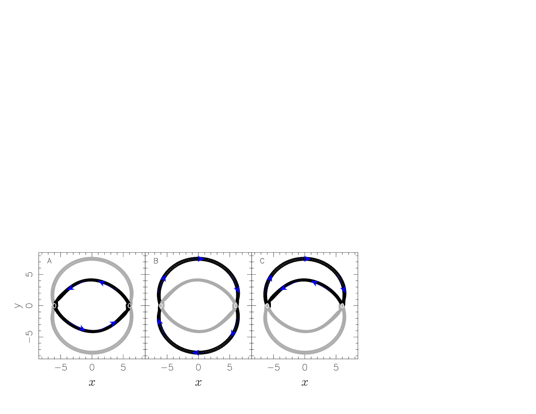
Figure 3: The four possible circulation patterns for particles on orbits guided by the manifolds. Any given such particle can stay on the inner branches of the manifold, i.e. can trace the inner ring (left panel), or it can stay on the outer branches of the manifold, i.e. can trace the outer ring (middle panel). Alternatively, it can trace a path that includes one inner and one outer branch. Two such paths are possible. One is shown in the right panel. The other, i.e. the fourth alternative, is not plotted here since it is similar to the third one, except that it is symmetric with respect to the bar major axis. After a particle has completed a full circulation path, it can either repeat the same path, or take any of the other three ones. The manifolds coming into play in each case are plotted in black in the corresponding panel, and the remaining ones in light grey. In white, we plot the Lyapunov periodic orbits of the corresponding energy level. The arrows show the direction of the motion.

This type of manifold morphology leads to interesting circulation patterns. Particles can follow essentially four different paths, shown in Fig. 3. One possibility is that they circulate along the inner branches of the invariant manifolds forming the inner ring (left panel of Fig. 3). This circulation is anti-clockwise. The second possibility is that they follow the outer branches of the manifolds, outlining the outer ring (middle panel of Fig. 3). This circulation is clock-wise. Finally, they can have a mixed trajectory, i.e. follow both inner and outer branches. Thus, particles starting from $L_{1}$ and following the inner branch of the unstable manifold approach the neighbourhood of $L_{2}$, move out of the bar region and follow the outer branch of the unstable manifold. They then reach a maximum distance from the centre and come back to the neighbourhood of $L_{1}$ (right panel of Fig. 3). In this way the circulation pattern is completed. A fourth circulation pattern (not shown in Fig. 3) has an identical shape but is reflected with respect to the bar major axis. In both the third and the fourth cases the circulation is clockwise with respect to their ‘centres’, i.e. with respect to the $L_{3}$ and $L_{4}$ Lagrangian points, respectively.

There are, thus, four circulation paths in total, one using only the inner branches, one using only the outer branches and two mixed ones, using both inner and outer branches. Once one such pattern is completed, a particle can either repeat it or take any of the other three circulation patterns. Thus, material from inside corotation can move outside it and vice-versa. However, the maximum radius such material can reach is bound by the maximum distance of the path from the centre, located on the direction of the bar minor axis.

As a second example, let us discuss a spiral morphology. Material, initially on an inner stable manifold branch, can, via the neighbourhood of one of the unstable Lagrangian points, move to an outer unstable branch. If this is of the escaping type (see previous section), we obtain a morphology similar to that of the grand design spiral arms of a barred galaxy.

The circulation pattern in this case is much simpler (Fig. 4). Matter from the inner region (more specifically from the outer regions of the bar or its immediate vicinity) moves along the inner manifolds towards one of the two unstable Lagrangian points and from there onto the corresponding outer branch of the unstable manifold. It can thus escape the inner region and reach outer parts of the disc.

Of course, an inwards going route could also be possible, at least in principle. Then matter from the outer parts of the disc could move inwards along a stable outer manifold branch to the $L_{1}$ or the $L_{2}$ and from there into the inner region. However, as will be discussed further in Sect. 7, the existence of a given manifold does not necessarily imply the existence of the corresponding structure in a galaxy, or in an $N$-body simulation. For this, the manifolds have to confine a sufficient amount of matter. This is similar to periodic orbits, where the existence of a stable family will not imply the formation of any structure if it does not trap any regular orbits around it. Thus the route bringing matter inwards, although in principle possible, would imply the existence of leading two-armed grand design spirals in barred potentials and has not yet been observed either in simulations or in real galaxies. Whether and how matter gets trapped by periodic orbits, or by manifolds depends on the formation history of the galaxy and is well beyond the scope of this paper. In Paper IV, however, we examine a few specific cases.

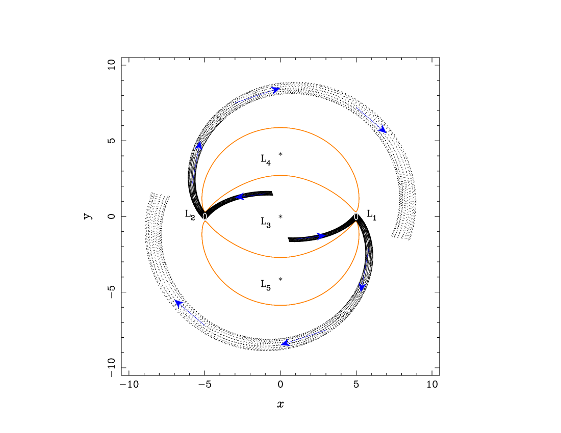
Figure 4: Circulation pattern for particles in models with spiral arms. The particle will move along the inner stable manifold branch and reaching the vicinity of one of the two unstable Lagrangian points will continue outwards along the unstable branch of the manifold. The direction of the motion is given by the arrows. We also plot the ZVC of the same energy as the manifolds (solid line) and give the position of the Lagrangian points with asterisks.

The two different morphological types discussed above, namely $rR_{1}$ rings and two-armed grand design spirals, do not come in the same potentials. The $rR_{1}$ morphology comes in models with bar potentials which are not too strong in the corotation region and immediately beyond it. In Paper III we gave, for the types of models of Sect. 2, upper limits of the bar strength beyond which this morphology will not occur. On the other hand, spirals form in models with stronger bar or appropriate spiral forcings. We also showed that it is the strength of the non-axisymmetric potential at and immediately beyond corotation that are the best indicators of the morphological type. For this we use the quantity

$$Q_{t}(r)=(\partial\Phi(r,\theta)/\partial\theta)_{max}/(r\partial\Phi_{0}/\partial r),$$ (2)

where $\Phi$ is the potential, $\Phi_{0}$ is its axisymmetric part and the maximum in the numerator is calculated over all values of the azimuthal angle $\theta$. We calculate $Q_{t}(r)$ at the radius of $L_{1}$, i.e. at $r=r_{L1}$ and denote it by $Q_{t,L_{1}}$. As shown in Paper III, $R_{1}$ morphologies form in models with relatively low values of $Q_{t,L_{1}}$, while higher values of this quantity give rise to other morphologies.

5 Cases with stable $L_{1}$ and $L_{2}$ Lagrangian points

5.1 Achieving stability

The morphologies and the characteristics of the invariant manifolds described so far assume that the $L_{1}$ and $L_{2}$ equilibrium points are unstable and with linear stability of the type “saddle$\times$centre$\times$centre”. We will hereafter refer to this case as the standard case. To make our theory more general, we also examine under what conditions the $L_{1}$ and $L_{2}$ can become stable and what consequences this will have on the galaxy morphology (Paper III).

It is possible to stabilise the equilibrium points by adding a concentration of matter around them. We tested this by adding two identical, small Kuz’min/Toomre discs (Kuz’min, 1956; Toomre, 1963), one centred on each of the $L_{1}$ and $L_{2}$. By increasing their mass, or decreasing their scale-length, the equilibrium point $L_{1}$ bifurcates, becoming stable, while two new unstable points appear, both on the direction of the bar major axis. They are located one on either side of $L_{1}$, and are called $L_{1}^{i}$ and $L_{1}^{o}$, the subscript, $i$ or $o$, denoting whether the corresponding new Lagrangian point is located inside or outside the $L_{1}$. Analogously, $L_{2}$ also becomes stable and two more unstable equilibrium points, $L_{2}^{i}$ and $L_{2}^{o}$, appear on either side of it. The mass of the added concentration at which this is attained is a decreasing function of its scale-length. Similarly, the concentration scale-length at which this is attained is an increasing function of its mass.

This new configuration is shown in Fig. 5, where we plot the ZVC for a given energy, the position of the equilibrium points and the outline of the bar, for model A with $a/b=2.5$, $r_{L}=6$, $Q_{m}=4.5\times 10^{4}$, and $\rho_{c}=2.4\times 10^{4}$. The scale-length and the mass of the two identical Kuz’min/Toomre discs are 0.6 and $0.025M_{b}$, respectively. The linear stability of the four new equilibrium points is of the type “saddle$\times$centre$\times$centre”, so we can compute the family of unstable periodic orbits and the manifolds associated to them, as we did for those of $L_{1}$ and $L_{2}$ in the standard case.

Figure 5: Location of the equilibrium points (marked with an asterisk) in an A model with $a/b=2.5$, $r_{L}=6$, $Q_{m}=4.5\times 10^{4}$ and $\rho_{c}=2.4\times 10^{4}$, to which have been added two identical Kuz’min/Toomre discs centred at the $L_{1}$ and $L_{2}$ Lagrangian points. The scale length and the mass of these discs are 0.6 and $0.025M_{b}$, respectively. The dashed line marks the position of the bar, while the dot-dashed lines show the zero velocity curves.

5.2 Global morphology

In Fig. 6 we compare the morphology obtained with the standard case to that with the same bar model plus the two mass concentrations around the $L_{1}$ and $L_{2}$ in the form of two small Kuz’min/Toomre discs. The two morphologies are essentially of the same type, since in both cases we obtain an $rR_{1}$ structure. However, the sizes and axial ratios of the two rings change drastically when the two mass concentrations are added and the number of equilibrium points increases to 9. The inner ring becomes smaller and is located very near the outline of the bar. Its axial ratio approaches that of the bar, while in the ‘standard’ case it has a smaller ellipticity. The major axis of the outer ring becomes much larger, and its axial ratio changes accordingly. If no material circulates between $L_{1}^{i}$ and $L_{1}^{o}$ and between $L_{2}^{i}$ and $L_{2}^{o}$, the inner and outer rings will not join, i.e. the outer ring will be detached. Such detached rings are often observed and this may be the way, or one of the ways, to explain their formation.

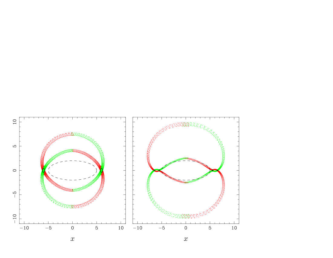
Figure 6: Comparison of the manifold morphology in the standard model with 5 equilibrium points (left panel, equilibrium points as in Fig. 1) and with 9 equilibrium points (right panel, equilibrium points as in Fig. 5). The bar outline is given by a dashed line and the corresponding Lyapunov orbits by a black solid line.

5.3 Specific morphology around the $L_{1}$ and $L_{2}$

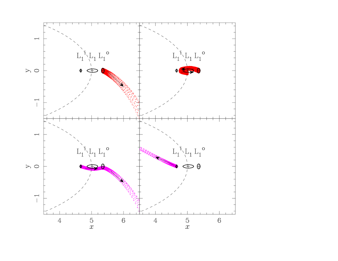
Figure 7: Morphology of the unstable manifold branches in the vicinity of a stable $L_{1}$ Lagrangian point (see text). The two upper panels show the manifolds linked to $L_{1}^{o}$ and the two lower ones those linked to $L_{1}^{i}$. The arrows show the direction of the motion around the manifolds and the dashed line shows the outline of the bar. Three periodic orbits – one around each of the $L_{1}$, $L_{1}^{i}$ and $L_{1}^{o}$ points – are given with solid lines.

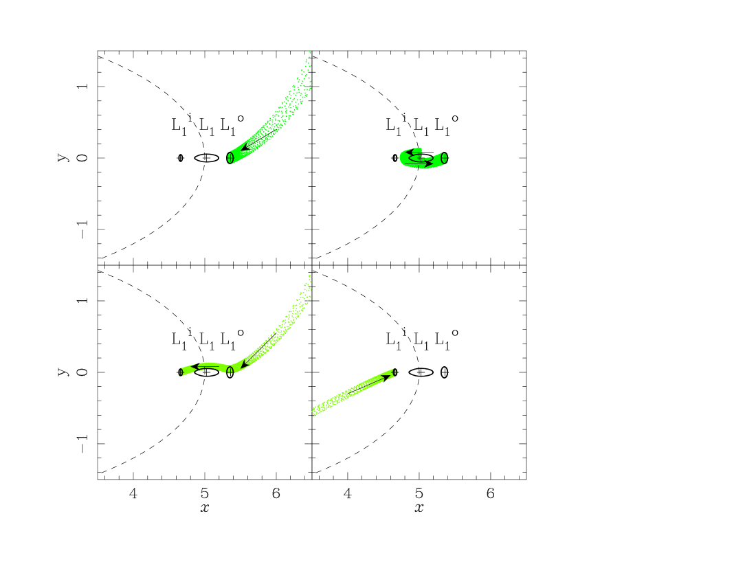
Figure 8: Same as Fig. 7, but for the stable branches of the manifolds.

The morphology of the unstable and stable manifolds in the immediate neighbourhood of the $L_{1}$ Lagrangian point is shown in Figs. 7 and 8, respectively, for a model which has a spiral morphology. This has several similarities, but also several differences from the model shown in Figs. 14 and 15 of Paper III, which is for a less strong bar with manifolds of $rR_{1}$ morphology.

The Lyapunov periodic orbits around $L_{1}$ are elongated in the same direction as the bar, while the periodic orbits around $L_{1}^{i}$ and $L_{1}^{o}$ are elongated perpendicular to it. It is the one around $L_{1}$ that is the largest and the one around $L_{1}^{i}$ that is the smallest, the third one being of intermediate size.

There are now in total four unstable branches (Fig. 7). The outer branch of the $L_{1}^{o}$ manifold, as well as the inner branch of the $L_{1}^{i}$ have a very simple morphology, while the two other branches have a more complicated and interesting morphology. The inner branch of the $L_{1}^{o}$ emanates from the vicinity of $L_{1}^{o}$ and circumventing the $L_{1}$ from the above extends towards $L_{1}^{i}$, but before reaching it turns back towards $L_{1}^{o}$, now circumventing the $L_{1}$ from below. The unstable outer branch of $L_{1}^{i}$ goes towards $L_{1}^{o}$ circumventing $L_{1}$ from below and then moves outwards beyond the corotation region. The morphology of the stable branches is similar and is shown in Fig. 8.

6 Ersatz for gas

Observations show that gas is intimately linked to both spirals and rings. For example, galaxies with smooth, very gas poor spiral arms, known as anemic, are a rarity (van den Bergh, 1976; Elmegreen et al., 2002). Furthermore, the formation of rings and spirals from gas has been witnessed in a number of simulations (e.g. Schwarz, 1981; Combes & Gerin, 1985; Athanassoula, 1992b; Lindblad, Lindblad & Athanassoula, 1996; Wada & Koda, 2001; Lin, Yuan & Buta, 2008; Rautiainen, Salo & Laurikainen, 2008). We should thus compare the dynamics of the gas with that of the manifolds presented here. Gas, however, has different equations of motion from stars, so we need to modify our calculations accordingly.

Schwarz (1979, 1981, 1984, 1985) uses sticky particles to simulate the gas and models collisions in a particularly straightforward way, so we can introduce a similar procedure also in our calculations. In Schwarz’s simulations, particles represent gaseous clouds which lose a certain fraction of their kinetic energy when they collide. In practise, they lose a certain fraction $f$ of their velocity (Schwarz, 1981), or only of the component of this velocity that is along the line joining the two particles (Schwarz, 1984, 1985). Thus, $v_{2}=\pm(1-f)v_{1}$, where $+$ is for the tranverse velocity component, $-$ is for the component along the line joining the two particles, and $v_{1}$ and $v_{2}$ are the velocities before and after the collision, respectively. The values of $f$ in Schwarz’s simulations range between 0.8 and 1.

We introduce collisions in our simulations in a similar way, thus obtaining an ersatz for gas, as described in more detail in Papers III and IV. We also use the same models as Schwarz in order to be able to make comparisons. Here we present results for his standard model with $a$ = 2.6, $q$ = 0.1, $\Omega_{p}$ = 0.27 and $f$ = 0.8, for which he gives sufficient results and information in his papers to allow comparisons, and which has an $rR_{1}$ manifold morphology. In this model we calculated a number of orbits of the outer branch of the unstable manifold and drew random numbers to find the locations along its trajectory where each particle will undergo a collision. In the particular example illustrated here we have three collisions per half bar rotation. We tried, however, different numbers of collisions, around the values used by Schwarz, and found qualitatively similar results.

To determine the result of a collision, we take a small box around the collision position and calculate the average velocity of all orbits in that box. We then decrease the velocity of the particle relative to that mean by a factor $\pm(1-f)$. Fig. 9 shows a comparison of the particle positions when they are considered as stellar (i.e. without collisions; grey) and as gaseous (with collisions; black). For this comparison we used $f$ = 0.8, which leads to a mean energy dissipation per particle of 1.25 $\times 10^{-3}$, in good agreement with the numbers given by Schwarz (1981). Other numerical values give qualitatively similar results. Fig. 9 shows that there is in general good agreement between the loci of the gaseous and of the stellar arm. Furthermore, the gaseous arm is more concentrated than the stellar arm, more so for a larger number of collisions per revolution.

Physically the above results can be understood as follows. Sticky particles (i.e. gaseous particles) follow the same orbits as the stellar ones, except at the time of the collisions. This ensures a general similarity. Due to the collisions, however, the gaseous particles lose part of their kinetic energy and their velocity approaches that of the mean. In Paper I, we compared the loci of manifolds for different energies and found that the ones with the smaller energies lie in configuration space within the ones with the higher energies. This means that the corresponding spiral arms, or rings will be thinner for the lower energies. Thus, when the particles lose energy they will fall onto an orbit nearer to the mean and the arms will become thinner. This is exactly what is found with the calculations leading to Fig. 9. Thus one can think of the lowest energy manifolds (i.e. the ones having the energy of $L_{1}$ and $L_{2}$) as an attractor, to which the gaseous trajectories will tend to because of the dissipation due to the collisions. Thus the gaseous arms should be thinner that the stellar ones, and this is indeed observed in real galaxies. This is discussed more extensively in Papers III and IV, where explicit comparisons are made.

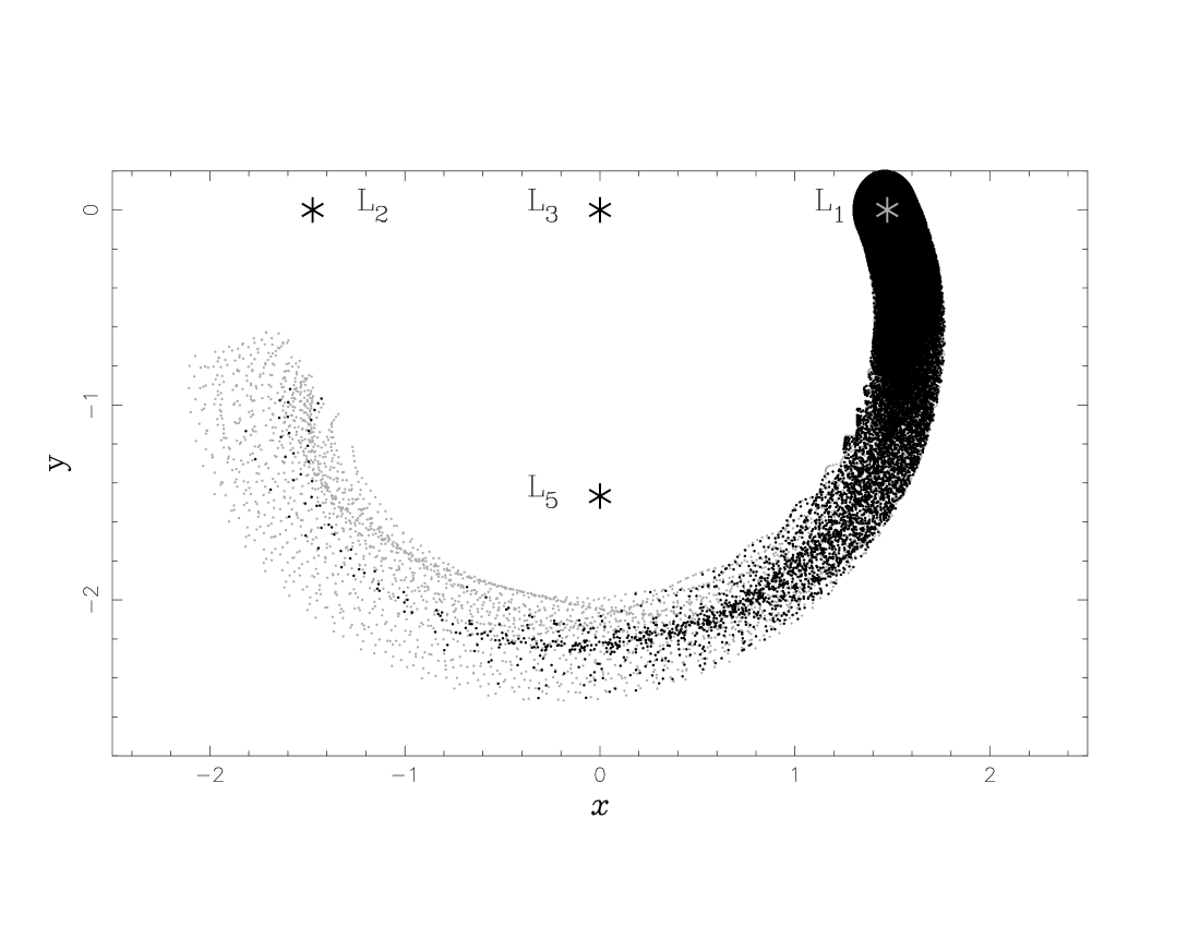
Figure 9: Comparison of the outer ring loci as calculated with (black) and without (grey) collisions. In this example $f$ = 0.8. The positions of the Lagrangian points are marked by asterisks. See text for a description of the calculations.

7 Final remarks

In this short review and, particularly, in the five papers on which it is based (Romero-Gómez et al., 2006, 2007, 2008; Athanassoula et al., 2008, and Athanassoula et al. 2009) we presented building blocks that can explain the formation of rings (both inner and outer) and spirals in barred galaxies. The invariant manifolds associated with the Lagrangian points $L_{1}$ and $L_{2}$ guide chaotic orbits which have the right shape for inner and outer rings and spirals and thus can be their building blocks. In particular, here we discussed morphologies of $rR_{1}$ type and of spiral type. We also discussed the case when the $L_{1}$ and $L_{2}$ are stable, and four other unstable points bifurcate from them. The whole structure then has nine Lagrangian points, five stable and four unstable. We also introduced an ersatz for gas and showed that the gaseous arms and the stellar arms should have roughly the same shape and that the former should be thinner than the latter.

Even though dynamically sound and very appealing, this theory will be useful for barred galaxies only if the manifolds and the orbits they guide create structures whose properties are in good agreement with observations. This point will be fully addressed in paper IV. Here let us just underline a couple of noteworthy points.

The first is that the existence of the manifolds, even if they have the right shape and properties, does not necessarily imply that the corresponding structures will be present in the galaxy. Indeed, the manifolds are only the building blocks, and the structure will be present only if some mass elements (e.g. stars) follow them. This is the same as for periodic orbits, which need to trap material around them to form the corresponding structure. Whether such material will exist or not depends on the formation and evolution of the galaxy (see Paper IV).

The second is that this is not the only theory attempting to explain spirals and rings, although most theories attempt either the one or the other. Our theory relies on the existence of a bar; in other cases a companion is necessary. The fact that a theory is correct and reproduces well many of the main observational data does not necessarily imply that all other theories are wrong, or irrelevant. Nor is it necessary in order to establish a theory to show that all others are wrong. Indeed spirals in different galaxies may have different origins, and even in the same galaxy more than one theory can be at work.