Bottom hadron mass splittings in the static limit from 2+1 flavour lattice QCD

Abstract

Dynamical 2+1 flavour lattice QCD is used to calculate the splittings between the masses of mesons and baryons containing a single static heavy quark and domain-wall light and strange quarks. Our calculations are based on the dynamical domain-wall gauge field configurations generated by the RBC and UKQCD collaborations at a spatial volume of (2.7 fm)³ and a range of quark masses with a lightest value corresponding to a (partially-quenched) pion mass of $275$ MeV. When extrapolated to the physical values of the light quark masses, the results of our calculations are generally in good agreement with experimental determinations in the bottom sector. However, the static limit splittings between the $\Omega_{b}^{-}$ baryon and other bottom hadrons tend to slightly underestimate those obtained using the recent D$0\!\!\!/$ measurement of the $\Omega_{b}^{-}$.

I Introduction

Hadrons containing a single bottom quark have received much attention recently. Over the last decade, the bottom meson sector has been investigated in great detail at the $b$ factories (BELLE and BaBar) and using the TeVatron at Fermilab. With the recent D$0\!\!\!/$ measurement of the $\Omega_{b}^{-}$ baryon Abazov:2008qm , we are rapidly approaching a complete picture of the ground-state bottom baryon sector as well. The start up of the Large Hadron Collider (LHC) will dramatically increase our knowledge of $b$ physics; both the dedicated $b$ physics experiment, LHCb, and the general purpose ATLAS and CMS experiments expect to observe unprecedented numbers of $b\overline{b}$ pairs, many of which will hadronise to bottom mesons and baryons.

In the bottom meson sector, many important observations have been made in the last decade, dramatically refining our knowledge of flavour physics. The CKM mechanism of the Standard Model currently provides a good description of current flavour-changing measurements of $B$ and $B_{s}$ mesons, bringing us into the precision era of flavour physics Barberio:2008fa . The various LHC experiments aim to investigate the decays of bottom baryons with enough precision to further test the Standard Model. In particular, the fact that bottom baryon polarisation can be measured may uncover new right-handed couplings. To search for physics beyond the Standard Model in these systems, it is necessary to have accurate predictions from the Standard Model. Typically, this requires non-perturbative evaluations of matrix elements from lattice QCD and thus an understanding of bottom hadrons in lattice QCD.

The simplest properties of the bottom hadrons are their masses. Before more complicated bottom observables can be predicted with any rigour, it is necessary to have reliable lattice calculations of the masses and mass splittings. There are many lattice studies of the mass of the $B$ mesons in the literature but fewer of the bottom baryons Bowler:1996ws ; AliKhan:1999yb ; Lewis:2001iz ; Mathur:2002ce and, only recently, the first unquenched bottom baryon calculations have appeared Na:2007pv ; Lewis:2008fu ; Burch:2008qx ; Na:2008hz . In this paper, we use light up and down quark masses to study the spectrum of bottom baryons and mesons. For the bottom quark, we work in the static ($m_{b}\to\infty$) limit. Since the bottom quark mass, $m_{b}\gg\Lambda_{\mathrm{QCD}}$, many properties of the physical bottom hadrons are expected to be close to those of hadrons containing a single, infinitely massive (static) quark, with corrections suppressed by powers of $\Lambda_{\mathrm{QCD}}/m_{b}$. Such corrections can be addressed systematically in Heavy Quark Effective Theory (see, e.g. Ref. Manohar:2000dt for a review). Our calculations use domain-wall fermions for the light and strange quarks and make use of the dynamical gauge configurations generated by the RBC and UKQCD collaborations using domain-wall quarks Antonio:2006px ; RBCUKQCD . We currently work at a single lattice spacing, $a=0.114$ fm RBCUKQCD and focus on a volume of spatial side, $L=2.74$ fm, for a range of quark masses corresponding to pion masses between 275 and 750 MeV.

This paper is organised in the following manner. In Section II, we present the details of the lattice calculations we have carried out. We discuss the mass splittings we observe in Section III before concluding in Section IV.

II Details of Lattice Calculations

The lattice QCD calculations presented here are based on the ensembles of 2+1 flavour lattices generated by the RBC and UKQCD collaborations Antonio:2006px ; RBCUKQCD . These ensembles use the Iwasaki gauge action Iwasaki:1984cj ; Iwasaki:1985we with $\beta=2.13$ and a domain wall quark action using the length of the fifth dimension, $L_{s}=16$. The parameters of the ensembles used this work are shown in Table 1 and we refer the reader to Ref. Antonio:2006px ; RBCUKQCD for further details.

Ensemble	$\beta$	Volume	$m_{\rm light}^{(sea)}$	$m_{\rm strange}^{(sea)}$	$m_{\rm res}$ RBCUKQCD	$N_{\rm cfgs}$
A	2.13	$24^{3}\times 64$	0.005	0.04	0.00315	$\sim 140$
B	2.13	$24^{3}\times 64$	0.01	0.04	0.00315	$\sim 180$
C	2.13	$24^{3}\times 64$	0.02	0.04	0.00320	$\sim 125$

Table 1: Parameters of the ensembles of RBC/UKQCD gauge configurations used in this calculation. For full details, see the original works, Refs. Antonio:2006px ; RBCUKQCD .

Using these ensembles, we have computed domain wall quark propagators Kaplan:1992bt ; Shamir:1992im ; Shamir:1993zy ; Shamir:1998ww ; Furman:1994ky for various different (partially quenched) quark masses as shown in Table 2. Our inversions use $L_{s}=16$ and a domain wall height of $M_{5}=1.8$ (note that these are the same parameters used in generating the ensembles and the bold entries in Table 2 correspond to QCD computations). To obtain clean signals, for the hadron energies and splittings, we use APE Teper:1987wt ; Albanese:1987ds smeared sources at multiple locations on each gauge configuration, performing a separate inversion for each source. The approximate masses of the pseudoscalar mesons computed with various combinations of these propagators are shown in Table 3.

Ensemble	$m_{\rm light}^{(val)}$	$N_{\rm cfg}$	$N_{\rm src}$
A	0.002	$\sim 140$	5
A	0.005	$\sim$ 140	6
A	0.01	$\sim 140$	1
A	0.02	$\sim 140$	1
A	0.03	$\sim 140$	1
A	0.04	$\sim$140	6
B	0.005	$\sim 180$	1
B	0.01	$\sim$180	5
B	0.02	$\sim 180$	1
B	0.03	$\sim 180$	1
B	0.04	$\sim$180	5
C	0.02	$\sim$125	1
C	0.04	$\sim$125	1

Table 2: Quark propagators used in calculations of the mass splittings. Bold entries denote $m_{\rm light}^{(val)}=m_{\rm light}^{(sea)}$. $N_{\rm src}$ indicates the number of sources that were used on each gauge configuration. These sources were spread around the lattice volume at as large relative separations as possible.

Ensemble	$m^{(\rm val)}_{\rm light}$	$m^{(\rm val)}_{\rm strange}$	$m^{(\rm val)}_{\pi}$ [GeV]	$m^{(\rm val)}_{K}$ [GeV]
A	0.002	0.04	0.275	0.560
A	0.005	0.04	0.331	0.576
A	0.01	0.04	0.415	0.602
A	0.02	0.04	0.546	0.654
A	0.03	0.04	0.653	0.701
A	0.04	0.04	0.747	—
B	0.005	0.04	0.335	0.581
B	0.01	0.04	0.419	0.607
B	0.02	0.04	0.550	0.657
B	0.03	0.04	0.657	0.706
B	0.04	0.04	0.751	—
C	0.02	0.04	0.549	0.654

Table 3: Approximate pion and kaon masses for each set of measurements.

The bottom quark is implemented in the static limit. Its propagator, $S_{Q}$ is represented as a product of gauge links in the temporal direction,

$$S_{Q}({\bf x},t;t_{0})=\left(\frac{1+\gamma_{4}}{2}\right)\prod_{t^{\prime}=t_{0}}^{t}U_{4}({\bf x},t^{\prime})\,,$$ (1)

where $U_{\mu}$ are SU(3) gauge links. At non-zero lattice spacing, there are different discretisations of the heavy quark action that have the same continuum limit. It is well-known (see e.g. Ref. DellaMorte:2003mn ) that signals for static hadron quantities are improved if the gauge links appearing in Eq. (1) are smeared in some manner over a small local volume. After extensive testing to optimise the heavy hadron signals, we perform our calculations with hypercubically-smeared (HYP) gauge links Hasenfratz:2001hp in the heavy quark propagator, Eq. (1). We study a number of choices of heavy quark smearing parameters as shown in Table 4, labelled $S_{i}$ for $i=0,\ldots,5$.

Set	$S_{0}$	$S_{1}$	$S_{2}$	$S_{3}$	$S_{4}$	$S_{5}$
$N_{\rm HYP}$	10	5	1	0	3	3
$\alpha_{1}$	0.75	0.75	0.75	0.75	0.75	0.6
$\alpha_{2}$	0.75	0.75	0.75	0.75	0.4	0.6
$\alpha_{3}$	0.75	0.75	0.75	0.75	0.65	0.6

Table 4: Parameters used in HYP-smearing the heavy quark action.

To extract the lattice energies, $E_{h}$, of the various hadrons, $h$, we compute the meson and baryon two-point correlation functions

$$C_{f}(t,t_{0}) = \sum_{{\bf x}}{\rm tr}\left[S_{Q}({\bf x},t;t_{0})S_{f}^{\dagger}({\bf x},t;{\bf x},t_{0})\right]\,,$$ (2)

$$C^{\Gamma}_{f,g}(t,t_{0}) = \sum_{{\bf x}}S^{k^{\prime}k}_{Q;\sigma\rho}({\bf x},t;t_{0})\epsilon^{ijk}\epsilon^{i^{\prime}j^{\prime}k^{\prime}}\left(S_{f}^{ii^{\prime}}({\bf x},t;{\bf x},t_{0})\Gamma\right)_{\rho\alpha}\left(\Gamma S_{g}^{jj^{\prime}}({\bf x},t;{\bf x},t_{0})\right)_{\sigma\alpha}\,,$$ (3)

for the various light flavour combinations, $f$($g$), and then combine them appropriately. The trace in the meson correlator is over color and spinor indices, and where explicit, the upper(additional lower) indices on the propagators correspond to colour(spin). For the baryons with the spin of the light degrees of freedom, $s_{\ell}$, being zero we choose $\Gamma=C\,\gamma_{5}$ where $C$ is the charge conjugation matrix, while for the baryons with $s_{\ell}=1$, we measure the three polarisations, corresponding to $\Gamma=C\,\gamma_{1,2,3}$, and average them in extracting the energies as they are degenerate in the infinite statistics limit. We combine the various correlators in Eq. (3) as appropriate for the specific SU(3) representation. For example, the $\Xi_{b}^{0}$ belongs to the flavour anti-triplet and is a $s_{\ell}=0$ state, consequently

$$C_{\Xi_{b}^{0}}=C^{\gamma_{5}}_{u,s}-C^{\gamma_{5}}_{s,u}$$ (4)

and similarly,

$$C_{\Lambda_{b}^{0}}=C^{\gamma_{5}}_{u,d}-C^{\gamma_{5}}_{d,u},\quad\quad C_{\Sigma_{b,i}^{0}}=C^{\gamma_{i}}_{u,d}+C^{\gamma_{i}}_{d,u},\quad\quad C_{\Xi_{b,i}^{\prime,0}}=C^{\gamma_{i}}_{u,s}+C^{\gamma_{i}}_{s,u},\quad\quad C_{\Omega_{b,i}^{-}}=C^{\gamma_{i}}_{s,s}\,.$$ (5)

As we work in the isospin limit, the other singly-heavy hadrons are degenerate with those above. In the static limit of the heavy quark, the $J^{P}=\frac{1}{2}^{+}$ states ($\Sigma_{b},\,\Xi_{b}^{\prime},\,\Omega_{b}$) and $\frac{3}{2}^{+}$ states ($\Sigma_{b}^{\ast},\,\Xi_{b}^{\prime\ast},\,\Omega_{b}^{\ast}$) are degenerate and our results correspond to this. Future calculations for $m_{b}\neq\infty$ will enable the spin splittings to be investigated, see Ref. Lewis:2008fu for recent work.

The transfer matrix formalism immediately shows that in the limit of large temporal separation, these correlators are dominated by exponentially decaying signal of the ground-state hadron energy. That is,

$$C_{h}(t,t_{0})\stackrel{{\scriptstyle t\gg t_{0}}}{{\longrightarrow}}A_{h}\exp{[-E_{h}(t-t_{0})]}\,,$$ (6)

where $E_{h}$ is the lattice energy. In the case of the $s_{\ell}=1$ baryons of strangeness $<2$, this is complicated by the fact that, at the physical quark masses and in infinite volume, they decay strongly to lighter $s_{\ell}=0,1$ baryons and a pion. For example, $\Sigma_{b}^{+}\to\Lambda_{b}\,\pi^{+}$ is the dominant decay mode Amsler:2008zz . However, at the unphysical masses and finite volumes used (the pion couples derivatively, requiring non-zero lattice momentum) here, these decays are forbidden. Additionally, the finite temporal extent (non-zero temperature) of the lattice geometry used in our calculations results in the appearance of exponentially suppressed states that decay with “lighter masses” that may pollute the signals of the zero temperature ground-state Detmold:2008aaa (this is asymmetric analog of the constant term expected in a two meson correlation function from one meson propagating forward in time and one propagating backward in time Detmold:2008yn ; Prelovsek:2008rf ). We will return to this issue below.

III Bottom Hadron Mass Splittings

In the static limit, the masses of bottom hadrons are infinite, however, the residual mass, $\overline{\Lambda}_{h}$, of a heavy hadron $h$ is well defined. In the lattice regularisation used here, the lattice energies, $E_{h}$ diverge as the continuum limit is taken and a perturbative subtraction is required to convert them to the corresponding residual mass, for example, in the modified minimal subtraction ($\overline{\rm MS}$) scheme. At one loop, this can be performed straightforwardly for typical lattice actions, and with more effort for the HYP-smeared gauge links used herein Loktik:2006kz ; Christ:2007cn . However, there are significant issues with higher order corrections and renormalons in the subtraction procedure Martinelli:1998vt ; Martinelli:1995vj . In contrast, the differences between the residual masses of two hadrons containing the same heavy quark (that is, the same lattice discretisation of a static quark) have well-defined continuum limits in which they are observable (the perturbative corrections and renormalisation scale dependence cancel in the difference). In our work, we concentrate on these differences and thereby avoid the issues mentioned above.

III.1 Heavy quark action

We first study the effects of the choice of the heavy quark action via the application of the various HYP-smearings shown in Table 4. For each energy or energy difference, the results for all the choices of smearing are found to be consistent within uncertainties. Figure 1 shows the noise-to-signal ratios for the correlators corresponding to the $\Sigma_{b}^{+}$—$B_{u}$, $\Omega_{b}^{-}$—$B_{s}$ and $\Xi_{b}^{0}$—$\Lambda_{b}$ mass splittings for the various smearing parameter sets as a function of Euclidean time using the QCD propagators of ensemble B in Table 1. As can be seen, the parameter set $S_{0}$ clearly has the strongest signals. The other sets of propagators display similar behaviour and we focus on set $S_{0}$ for the remainder of our study.

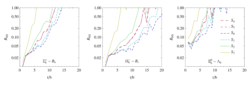
Figure 1: The ratio of noise to signal, $R_{NS}$, for exemplary correlator differences for the different choices of the heavy quark action (Table 4). The $m^{(\rm val)}=m^{(\rm sea)}$ quark propagators on the B ensemble were used in this comparison. The other sets display similar behaviour.

III.2 Analysis Methods

To extract the mass differences from the lattice correlators defined in the previous section, we perform multiple independent analyses using different methods. We fit to either single- or two-state effective masses and /or mass differences(see Ref. Fleming:2004hs ), or perform multi-exponential fits to (differences of) correlation functions using Bayesian priors (as in Refs Lepage:2001ym ; Wingate:2002fh ). We use the bootstrap analysis method to estimate our uncertainties. We average over all propagators computed from the various sources on each configuration and then bin the measurements over units of $\sim$100 molecular dynamics time units as residual correlations are observed to persist over this range RBCUKQCD . The number of bootstrap ensembles used in our analysis is typically four times the number of binned measurements, $N_{\rm bootstrap}\sim 200$.

Correlation functions are calculated with both an APE smeared sink (using the same parameters as at the source) or a point sink. Results from both sink types are consistent. In general, the fitting to the energy differences leads to a cleaner signal than fitting each energy individually, but not in all cases and both approaches were tried.

In the correlated fits to single- and two-state effective masses, a systematic uncertainty is assigned from varying the fitting ranges, $t_{\rm min}$ to $t_{\rm max}$, or from differences between fits to sliding windows of time-slices within the overall fit range. Typically, single effective masses are fit from $t_{\rm min}\sim 9$ and two-state effective masses are fit from $t_{\rm min}\sim 4$ (here, the ground state plateaus earlier as the excited state contamination is decreased significantly). The upper limit of the fits is $t_{\rm max}\sim 20$ for mesons and anti-triplet baryons, and $t_{\rm max}\sim 15$ for sextet baryons where states arising from the finite temporal extent discussed above pollute the signal.

In the Bayesian analysis, the correlation functions are fit to

$$C(t)~{}=~{}A_{1}e^{-E_{1}t}(1+B_{1}e^{-\Delta E_{1}t}+B_{2}e^{-(\Delta E_{1}+\Delta E_{2})t})+A_{1}C_{1}e^{-E^{\prime}t}\,.$$ (7)

over the range $2\leq t\leq 20$. This form was sufficient to provide an acceptable fit to all correlators and additional exponential terms were not constrained by the data. The Bayesian prior distribution functions are Gaussian. The mean values for the $A_{1}$ and $E_{1}$ priors were estimated from single exponential fits at large times. The widths for those parameters were taken to be about 50% and 10%, respectively, are significantly larger than the uncertainties from the initial single exponential fit. The mean values for the $B_{i}$ priors were in $[-1,1]$ with widths up to a factor 10, and the $\Delta E_{i}$ priors had means in $[0.3,0.6]$ with widths between 60% and 80%. The last term in (7) allows for contributions to $C(t)$ due to multi-particle states created by the interpolating operators in Eq (2) and (3). Usually these states give vanishingly small contribution, as their total energy is greater than the hadron mass of interest. However, with (anti-)periodic boundary conditions in $t$, these states can contaminate the large $t$ behavior due to a backward propagating light meson Detmold:2008aaa . Therefore we include the last term in Eq. (7) with prior mean for $C_{1}\approx\exp(-0.1\,T)$, where $T$ is the temporal extent of the lattice, and for $E^{\prime}=0.5$, both with 100% widths.

In combining the various analyses, we make a direct comparison of the various extractions and if they are in agreement, we take their mean. If there are discrepancies (very few are found), we assign an additional systematic uncertainty large enough to make the result consistent with the individual analyses.

The final results of our analyses of the lattice calculations are shown in Fig. 2 for the various quark masses on the three ensembles (the statistical, and all systematic uncertainties have been combined in quadrature). The empty points correspond to calculations that are partially quenched, with the sea quark masses differing from the valence quark masses. Ensembles A, B and C are coloured blue, red and green respectively.

III.3 Quark mass extrapolations

The light quark mass dependence of the static hadron energies and mass differences calculated in this work is, at least in principle, described by the low energy effective theory, heavy hadron chiral perturbation theory (HH$\chi$PT) Burdman:1992gh ; Wise:1992hn ; Yan:1992gz ; Cho:1992gg ; Cho:1992cf or its quenched and partially-quenched versions Savage:1995dw ; Chiladze:1997uq ; Tiburzi:2004kd . In addition to polynomial dependence on the pion and kaon masses, non-analytic terms such as $m_{\pi}^{2}\log[m_{\pi}^{2}/\mu^{2}]$ appear ($\mu$ is the renormalisation scale). We have attempted to perform extrapolations using the forms predicted by these theories. Unfortunately, our current data are insufficient to constrain the coefficients of the non-analytic terms in the HH$\chi$PT expressions (three axial couplings contribute in the coefficients of the non-analytic terms in the various differences). Future, direct calculations of the axial couplings will enable a more controlled chiral extrapolation.

With this in mind, here we use simple polynomial fits to perform the light quark mass extrapolations, allowing linear, quadratic and cubic dependence on $m_{q}\sim m_{\pi}^{2}$. Since we keep $m_{s}$ fixed, we do not include dependence on this parameter (we note that it is not quite tuned to the physical value RBCUKQCD ). These fits use a maximum likelihood estimator and are performed in an uncorrelated manner for simplicity. Accounting for the correlations between the different partially-quenched data points computed on the same underlying ensemble would slightly reduce our uncertainty. However, given the extrapolation forms used at present are ad hoc, we do not pursue this further. The resulting $\chi^{2}$s of the fits are all acceptable.

We have also performed coupled fits to all the differences, allowing a fixed polynomial dependence on $m_{\pi}$ for each of the hadron energies. This coupled fitting procedure provides a successful fit and agrees with the above (uncoupled) method within uncertainties but does not improve the extrapolations.

In Fig. 2, we show the results of the linear (blue), quadratic (red) and cubic (green) fits to the data contained in the ordinate extent of corresponding shaded region. The extracted splittings at the physical light quark masses are presented in Table 5 for each extrapolation and compared to experimental determinations where available. Differences between the three forms of extrapolations are relatively small, and, as an example, the linearly extrapolated mass differences are shown in Fig 3 along with the experimental determinations.

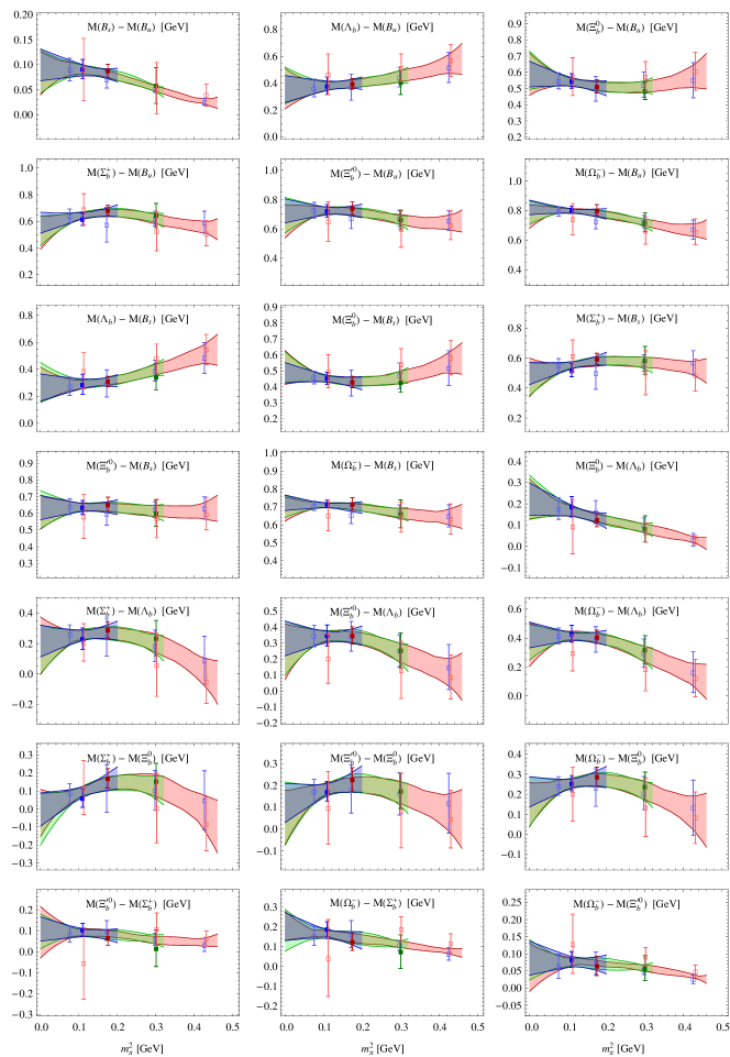
Figure 2: Polynomial extrapolations of the mass splittings calculated on the various ensembles are shown as a function of the pion mass. The blue, red and green points correspond to ensembles A, B and C respectively. Solid (open) symbols denote QCD (partially-quenched QCD) calculations. The uncertainties on the lattice data combine the statistical uncertainties and the various systematic uncertainties in quadrature. The blue, green and red shaded regions show the one standard deviation allowed region of linear, quadratic and cubic fits to the data within the ordinate extent of the corresponding region.

$h_{1}$	$h_{2}$	$M_{h_{1}}-M_{h_{2}}$ (lin.)	$M_{h_{1}}-M_{h_{2}}$ (quad.)	$M_{h_{1}}-M_{h_{2}}$ (cub.)	$M_{h_{1}}-M_{h_{2}}$ (expt.)
$B_{s}$	$B_{u}$	0.097(28)	0.092(35)	0.084(32)	0.0867(11)
$\Lambda_{b}$	$B_{u}$	0.362(88)	0.37(11)	0.36(12)	0.3407(20)
$\Lambda_{b}$	$B_{s}$	0.271(88)	0.28(12)	0.29(10)	0.2540(22)
$\Xi_{b}^{0}$	$B_{u}$	0.579(69)	0.595(94)	0.588(98)	0.5136(30)
$\Xi_{b}^{0}$	$B_{s}$	0.482(55)	0.500(75)	0.502(82)	0.4269(32)
$\Xi_{b}^{0}$	$\Lambda_{b}$	0.214(67)	0.211(86)	0.212(76)	0.1729(36)
$\Sigma_{b}^{+}$	$B_{u}$	0.600(68)	0.564(89)	0.556(93)	0.5322(30)
$\Sigma_{b}^{+}$	$B_{s}$	0.508(64)	0.484(88)	0.491(96)	0.4455(32)
$\Sigma_{b}^{+}$	$\Lambda_{b}$	0.222(90)	0.19(13)	0.21(14)	0.1915(36)
$\Sigma_{b}^{+}$	$\Xi_{b}^{0}$	0.012(80)	-0.02(11)	-0.002(93)	0.0186(42)
$\Xi_{b}^{\prime 0}$	$B_{u}$	0.718(71)	0.698(98)	0.677(90)	—
$\Xi_{b}^{\prime 0}$	$B_{s}$	0.633(64)	0.622(91)	0.616(79)	—
$\Xi_{b}^{\prime 0}$	$\Lambda_{b}$	0.332(94)	0.30(13)	0.27(13)	—
$\Xi_{b}^{\prime 0}$	$\Xi_{b}^{0}$	0.131(78)	0.10(11)	0.094(95)	—
$\Xi_{b}^{\prime 0}$	$\Sigma_{b}^{+}$	0.102(50)	0.094(64)	0.079(92)	—
$\Omega_{b}^{-}$	$B_{u}$	0.817(42)	0.794(61)	0.776(58)	0.886(15)
$\Omega_{b}^{-}$	$B_{s}$	0.718(37)	0.705(48)	0.696(51)	0.799(15)
$\Omega_{b}^{-}$	$\Lambda_{b}$	0.419(78)	0.385(98)	0.37(11)	0.545(15)
$\Omega_{b}^{-}$	$\Xi_{b}^{0}$	0.222(65)	0.182(97)	0.175(83)	0.372(15)
$\Omega_{b}^{-}$	$\Sigma_{b}^{+}$	0.196(61)	0.181(82)	0.173(55)	0.354(15)
$\Omega_{b}^{-}$	$\Xi_{b}^{\prime 0}$	0.086(43)	0.084(47)	0.076(55)	—

Table 5: Extracted static limit mass differences [GeV] obtained through linear, quadratic or cubic extrapolations in $m_{\pi}^{2}$ to its physical value. The uncertainties in the extrapolated values correspond to one standard deviation allowed region of the space of fit parameters. Experimental mass splittings Amsler:2008zz ; Abazov:2008qm are shown for comparison (for the mesons and the sextet baryons, we report the lighter of the heavy quark spin multiplets). The $\Xi_{b}^{\prime 0}$ has not been observed.

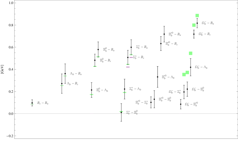
Figure 3: SU(3) mass splittings between bottom hadrons linearly extrapolated to the physical light quark masses. The green shaded regions correspond to the experimental determinations (combinations with both the $B_{u,s}^{\ast}$ and the $\Sigma_{b}^{\ast+}$ are shown in purple).

IV Conclusions and Outlook

In this paper, we have presented a study of the mass splittings between mesons and baryons containing one static quark using lattice calculations based on the domain-wall fermion RBC/UKQCD ensembles. We have used domain wall quarks with a range of masses, the lightest set corresponding to a pion mass of $\sim$275 MeV and at a single lattice spacing, $a=0.114$ fm. In general, the splittings we extract agree well with experiment. Those involving the $\Omega_{b}^{-}$ tend to be smaller than found experimentally as also found recently in the lattice calculations of Refs. Lewis:2008fu ; Burch:2008qx , but the discrepancy is barely significant at our current level of precision once the quark mass extrapolations are accounted for.

Our chiral extrapolations are somewhat ad hoc at present as the axial couplings between $b$-hadrons and light pseudoscalar mesons that appear in HH$\chi$PT are relatively unknown, making extrapolations using the results of chiral perturbation theory problematic. Ongoing calculations of these charges will allow us to control better the mass difference extrapolations. Additionally, the effects of the slightly unphysical strange quark mass need to be accounted for. Our calculations are performed in the static limit of the $b$ quark and so our extracted values for the splittings are subject to uncertainties ${\cal O}(\Lambda_{\rm QCD}/m_{b})$ when compared to the experimental bottom hadron spectrum. In the future, we intend to revisit these calculations using either non-relativistic QCD or the Fermilab heavy quark formalism. We also intend to extend our calculations to other lattice spacings and volumes as they become available.

- (1) V. M. Abazov et al. [D0 Collaboration], arXiv:0808.4142 [hep-ex].
- (2) E. Barberio et al. [Heavy Flavor Averaging Group], arXiv:0808.1297 [hep-ex].
- (3) K. C. Bowler et al. [UKQCD Collaboration], Phys. Rev. D 54, 3619 (1996) [arXiv:hep-lat/9601022].
- (4) A. Ali Khan et al., Phys. Rev. D 62, 054505 (2000) [arXiv:hep-lat/9912034].
- (5) R. Lewis, N. Mathur and R. M. Woloshyn, Phys. Rev. D 64, 094509 (2001) [arXiv:hep-ph/0107037].
- (6) N. Mathur, R. Lewis and R. M. Woloshyn, Phys. Rev. D 66, 014502 (2002) [arXiv:hep-ph/0203253].
- (7) H. Na and S. A. Gottlieb, PoS LAT2007, 124 (2007) [arXiv:0710.1422 [hep-lat]].
- (8) R. Lewis and R. M. Woloshyn, arXiv:0806.4783 [hep-lat].
- (9) T. Burch, C. Hagen, C. B. Lang, M. Limmer and A. Schafer, arXiv:0809.1103 [hep-lat].
- (10) H. Na and S. Gottlieb, arXiv:0812.1235 [hep-lat].
- (11) A. V. Manohar and M. B. Wise, Camb. Monogr. Part. Phys. Nucl. Phys. Cosmol. 10, 1 (2000).
- (12) D. J. Antonio et al. [RBC and UKQCD Collaborations], Phys. Rev. D 75, 114501 (2007).
- (13) C. Allton et al., Phys. Rev. D76 (2007) 014504; C. Allton et al., arXiv:0804.0473 [hep-lat].
- (14) Y. Iwasaki and T. Yoshie, Phys. Lett. B 143, 449 (1984).
- (15) Y. Iwasaki, Nucl. Phys. B 258, 141 (1985).
- (16) D. B. Kaplan, Phys. Lett. B 288, 342 (1992) [arXiv:hep-lat/9206013].
- (17) Y. Shamir, Phys. Lett. B 305, 357 (1993) [arXiv:hep-lat/9212010].
- (18) Y. Shamir, Nucl. Phys. B 406, 90 (1993) [arXiv:hep-lat/9303005].
- (19) V. Furman and Y. Shamir, Nucl. Phys. B 439, 54 (1995) [arXiv:hep-lat/9405004].
- (20) Y. Shamir, Phys. Rev. D 59, 054506 (1999) [arXiv:hep-lat/9807012].
- (21) M. Teper, Phys. Lett. B 183, 345 (1987).
- (22) M. Albanese et al., Phys. Lett. B 192, 163 (1987).
- (23) M. Della Morte et al.,[ALPHA Collaboration], Phys. Lett. B 581, 93 (2004).
- (24) A. Hasenfratz and F. Knechtli, Phys. Rev. D 64, 034504 (2001) [arXiv:hep-lat/0103029].
- (25) C. Amsler et al. [Particle Data Group], Phys. Lett. B 667, 1 (2008).
- (26) W. Detmold et al., [NPLQCD Collaboration], in preparation.
- (27) W. Detmold, K. Orginos, M. J. Savage and A. Walker-Loud, Phys. Rev. D 78, 054514 (2008).
- (28) S. Prelovsek and D. Mohler, arXiv:0810.1759 [hep-lat].
- (29) O. Loktik and T. Izubuchi, Phys. Rev. D 75, 034504 (2007) [arXiv:hep-lat/0612022].
- (30) N. H. Christ, T. T. Dumitrescu, O. Loktik and T. Izubuchi, PoS LAT2007, 351 (2007).
- (31) G. Martinelli and C. T. Sachrajda, Nucl. Phys. B 559, 429 (1999) [arXiv:hep-lat/9812001].
- (32) G. Martinelli and C. T. Sachrajda, Phys. Lett. B 354, 423 (1995) [arXiv:hep-ph/9502352].
- (33) G. T. Fleming, arXiv:hep-lat/0403023.
- (34) M. Wingate et al.,Phys. Rev. D 67, 054505 (2003) [arXiv:hep-lat/0211014].
- (35) G. P. Lepage et al., Nucl. Phys. Proc. Suppl. 106, 12 (2002) [arXiv:hep-lat/0110175].
- (36) G. Burdman and J. F. Donoghue, Phys. Lett. B 280, 287 (1992).
- (37) M. B. Wise, Phys. Rev. D 45, 2188 (1992).
- (38) T. M. Yan et al., Phys. Rev. D 46, 1148 (1992) [Erratum-ibid. D 55, 5851 (1997)].
- (39) P. L. Cho, Phys. Lett. B 285, 145 (1992) [arXiv:hep-ph/9203225].
- (40) P. L. Cho, Nucl. Phys. B 396, 183 (1993) [Erratum-ibid. B 421, 683 (1994)] [arXiv:hep-ph/9208244].
- (41) M. J. Savage, Phys. Lett. B 359, 189 (1995) [arXiv:hep-ph/9508268].
- (42) G. Chiladze, Phys. Rev. D 57, 5586 (1998) [arXiv:hep-ph/9704426].
- (43) B. C. Tiburzi, Phys. Rev. D 71, 034501 (2005) [arXiv:hep-lat/0410033].
- (44) R. G. Edwards and B. Joo, Nucl. Phys. Proc. Suppl. 140 (2005) 832; C. McClendon, ”Optimized Lattice QCD Kernels for a Pentium 4 Cluster”, Jlab preprint, JLAB-THY-01-29.