Improved spacecraft radio science using an on-board atomic clock:
application to gravitational wave searches

Abstract

Recent advances in space-qualified atomic clocks (low-mass, low power-consumption, frequency stability comparable to that of ground-based clocks) can enable interplanetary spacecraft radio science experiments at unprecedented Doppler sensitivities. The addition of an on-board digital receiver would allow the up- and down-link Doppler frequencies to be measured separately. Such separate, high-quality measurements allow optimal data combinations that suppress the currently-leading noise sources: phase scintillation noise from the Earth’s atmosphere and Doppler noise caused by mechanical vibrations of the ground antenna. Here we provide a general expression for the optimal combination of ground and on-board Doppler data and compute the sensitivity such a system would have to low-frequency gravitational waves (GWs). Assuming a plasma scintillation noise calibration comparable to that already demonstrated with the multi-link CASSINI radio system, the space-clock/digital-receiver instrumentation enhancements would give GW strain sensitivity of $2.0\times 10^{-17}$ for randomly polarized, monochromatic GW signals over a two-decade ($\sim 0.0001-0.01$ Hz) region of the low-frequency band. This is about an order of magnitude better than currently achieved with traditional two-way coherent Doppler experiments. The utility of optimally combining simultaneous up- and down-link observations is not limited to GW searches. The Doppler tracking technique discussed here could be performed at minimal incremental cost to also improve other radio science experiments (i.e. tests of relativistic gravity, planetary and satellite gravity field measurements, atmospheric and ring occultations) on future interplanetary missions.

I Introduction

Measurements of the relative velocity between the Earth and an interplanetary spacecraft, by means of coherent microwave tracking, have allowed studies of solar system bodies kliore_etal2004 , tests of relativistic gravity Vessot1993 ; bertotti_etal2003 , searches for low-frequency gravitational radiation EW1975 ; Tinto1996 ; Armstrong2006 , and other science objectives kliore_etal2004 . In the frequency band ($10^{-6}-10^{-2}$) Hz, typical deep space tracks are limited by phase scintillation caused by random refractivity variations in the solar wind, and the ionosphere asmar_etal2005 . The most sensitive deep-space Doppler observations to date, however, calibrate and largely remove these noises bertotti_etal1993 ; Tinto2002 ; bertotti_etal2003 ; armstrong_etal2003 and are then limited by antenna mechanical noise (unmodeled motion of the phase center of the ground antenna) and residual post-calibration tropospheric scintillation (i.e. Doppler fluctuations caused by refractive index fluctuations in the Earth’s atmosphere) Tinto1996 ; asmar_etal2005 . The most sensitive observations hit the limit identified by these noise sources with an Allan standard deviation of about $3\times 10^{-15}$ for integration times of a few thousand seconds. Improved sensitivity would benefit the science disciplines listed above, but antenna mechanical noise, in particular, has seemed irreducible at reasonable cost since it would require a large, moving, steel structure much more rigid than that of the current ground tracking stations.

Several ideas have been proposed to reduce the antenna mechanical noise or the tropospheric noise, or both Armstrong_Estabrook_etal . Those ideas do not involve modifications to the spacecraft, but rather use simultaneous tracking on the ground with appropriate linear combinations of those data to synthesize an observable with the ground/tropospheric noises of the better of the two receiving stations. If, however, additional microwave instrumentation on the spacecraft is considered, such as a space-borne, high-stability frequency standard Prestage_Weaver2007 ; Dick1990 and a space-qualified digital receiver Tyler_etal_2008 ; RASSI_2008 , then an alternative method for noise suppression is possible. This involves properly combining the two one-way (spacecraft to Earth and simultaneous Earth to spacecraft) Doppler data taken onboard and on the ground in such a way to maximize the signal-to-noise ratio of the observed physical observable. Multiple Doppler observations with different noises, or different transfer functions to the same noises, are clearly useful in identifying noise sources and minimizing (and in some cases canceling) their effects on the final observable. In particular, the use of multiple radio links (some of which driven by a high-quality space-borne frequency standard) was pioneered by R. Vessot in the Gravity Probe A sub-orbital experiment Vessot1970 . Because of mass and power constraints, however, no very high quality frequency standards have yet been flown on deep space probes.

Recent advances in clock technology indicate that a new era of space-qualified, highly stable frequency standards has started Prestage_Weaver2007 , which will result into significantly improved Doppler radio science experiments. A summary of this paper is given below.

In Section II we present a brief overview of the theory underlying Doppler tracking experiments relying only on the two one-way Doppler data measured onboard and on the ground. Although this experimental configuration has been discussed in previous publications Vessot1970 ; Piran_etal1986 , it has been shown only relatively recently Tinto1996 ; Tinto2002 how to fully take advantage of it for improving the precision of Doppler tracking radio science experiments. A brief description of an onboard atomic clock and a digital receiver is given in the Appendix, where an account of all the one-sided power spectral densities of the noises affecting the Doppler data is also presented.

The main advantage of spacecraft Doppler tracking experiments relying on the two one-way Doppler data, over those based on two-way coherent measurements, is in their ability of exactly canceling the frequency fluctuations due to the Earth atmosphere and ionosphere, and the mechanical vibrations of the ground antenna, presently the main noise sources of Doppler tracking experiments Tinto1996 . This is possible because there exists a unique linear combination of the properly time-shifted one-way measurements that does exactly that Tinto1996 . Depending on the specific radio science experiment performed with this technique, it is actually possible to combine optimally the two one-way Doppler measurements to maximize the signal-to-noise ratio (SNR) of the experiment. After deriving the expression of the optimal SNR in Section III, we apply it to searches for gravitational waves. Under the assumption of calibrating the frequency fluctuations induced by the interplanetary plasma, we find that a Doppler broad-band sensitivity of $2.0\times 10^{-17}$ to randomly polarized monochromatic signals uniformly distributed over the sky can be achieved. This is about one order of magnitude better than that obtainable with two-way coherent Doppler tracking experiments. Narrow-band searches at frequencies where the transfer function of the onboard clock reaches sharp nulls (i.e. the “xylophone” frequencies) Tinto1996 further enhance the strain sensitivity of these experiments to about $7.0\times 10^{-18}$.

In Section IV we finally present our comments and conclusions, and emphasize that the Doppler tracking technique discussed in this article can be performed at minimal additional cost by forthcoming interplanetary missions.

II The One-Way Doppler Tracking Observables

In Doppler tracking experiments aimed at detecting low-frequency (milliHertz) gravitational radiation, a distant interplanetary spacecraft is monitored from Earth through a radio link, with the Earth and the spacecraft acting as free-falling test particles . A radio signal of nominal frequency $\nu_{0}$ is transmitted to the spacecraft, and coherently transponded back to Earth where the received signal is compared to a signal referenced to a highly stable clock (typically a hydrogen-maser). Relative frequency changes $\Delta\nu/\nu_{0}$, as functions of time, are measured. When a gravitational wave crossing the solar system propagates through the radio link, it causes small perturbations in $\Delta\nu/\nu_{0}$, which are replicated three times in the Doppler data with maximum spacing given by the two-way light propagation time between the Earth and the spacecraft EW1975 .

An alternative way of performing Doppler tracking searches for gravitational radiation was suggested in Vessot_Levine1978 ; Piran_etal1986 ; Tinto1996 . By adding a highly-stable clock and a digital receiver to the spacecraft radio instrumentation (Figure 1), two one-way Doppler time series can be recorded simultaneously at the ground station and on board the spacecraft.

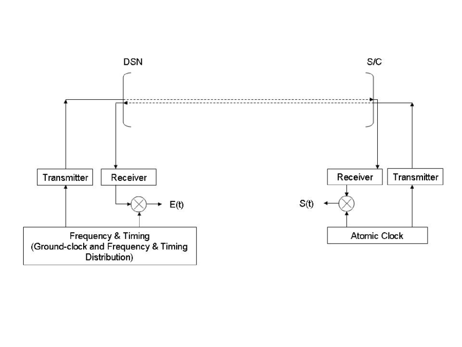
Figure 1: Block diagram of the radio hardware at the ground antenna of the NASA Deep Space Network (DSN) and on board the spacecraft (S/C), which allows the acquisition and recording of the two Doppler data $E(t)$, $S(t)$. A description of each individual block in this diagram is provided in the Appendix.

If we introduce a set of Cartesian orthogonal coordinates ($X,Y,Z$) in which the wave is propagating along the $Z$-axis and ($X,Y$) are two orthogonal axes in the plane of the wave (see Figure 2), then the two one-way relative frequency fluctuations at time $t$ can be written in the following form after first-order Doppler and other systematic Doppler effects are modeled out from the data Tinto1996

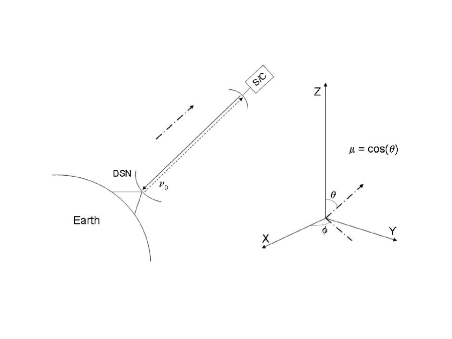
Figure 2: A radio signal of nominal frequency $\nu_{0}$ is transmitted to a spacecraft and simultaneously another radio signal from the spacecraft and referenced to the onboard clock is transmitted to the ground. The gravitational wave train propagates along the $Z$ direction, and the cosine of the angle between its direction of propagation and the radio beam is denoted by $\mu$. See text for a complete description.

$$\left(\frac{\Delta\nu(t)}{\nu_{0}}\right)_{E}\equiv E(t) = \frac{1-\mu}{2}\ \left[h(t-(1+\mu)L)\ -\ h(t)\right]\ +\ C_{S}(t-L)\ -\ C_{E}(t)$$ (1)

$$+ T(t)\ +\ B(t-L)\ +\ A_{S}(t-L)\ +\ EL_{E}(t)\ +\ P_{E}(t)\ ,$$

$$\left(\frac{\Delta\nu(t)}{\nu_{0}}\right)_{S}\equiv S(t) = \frac{1+\mu}{2}\ \left[h(t-L)\ -\ h(t-\mu L)\right]\ +\ C_{E}(t-L)\ -\ C_{S}(t)$$ (2)

$$+ T(t-L)\ +\ B(t)\ +\ A_{E}(t-L)\ +\ EL_{S}(t)\ +\ P_{S}(t)\ ,$$

where $h(t)$ is equal to

$$h(t)=h_{+}(t)\cos(2\phi)+h_{\times}(t)\sin(2\phi)\ .$$ (3)

Here $h_{+}(t)$, $h_{\times}(t)$ are the wave’s two amplitudes with respect to the ($X,Y$) axis, ($\theta,\phi$) are the polar angles describing the location of the spacecraft with respect to the ($X,Y,Z$) coordinates, $\mu$ is equal to $\cos\theta$, and $L$ is the distance to the spacecraft (units in which the speed of light $c=1$)

In Eqs. (1, 2) we have assumed the Earth and the on board clocks to be perfectly synchronized. Although this condition is impossible to achieve in practice, it has been previously shown by one of us Tinto2002 that the accuracy required for successfully implementing a noise cancellation scheme similar to the one discussed in this paper requires a clock synchronization accuracy of about $0.5\ s$, which is easy to achieve.

In Eqs. (1,2) we have denoted by $C_{E}(t)$, $C_{S}(t)$ the random processes associated with the frequency fluctuations of the clock on Earth and onboard respectively, $B(t)$ the joint effect of the noise from buffeting of the probe by non gravitational forces and from the antenna of the spacecraft, $T(t)$ the joint frequency fluctuations due to the troposphere, ionosphere and ground antenna, $A_{E}(t)$ the noise of the radio transmitter on the ground, $A_{S}(t)$ the noise of the radio transmitter on board, $EL_{E}(t)$, $EL_{S}(t)$, the noise from the electronics on the ground and onboard respectively, and $P_{E}(t)$, $P_{S}(t)$ the fluctuations on the two links due to the interplanetary plasma. Since the frequency fluctuations induced by the plasma are, to first order, inversely proportional to the square of the radio frequency, by using high frequency radio signals or by monitoring two different radio frequencies transmitted to and from the spacecraft, this noise source can be suppressed to very low levels or entirely removed from the data respectively bertotti_etal1993 . In what follows we will assume dual frequency to be used, and disregard the noise effects of the plasma fluctuations in our analysis.

From Eqs. (1,2) we deduce that gravitational wave pulses of duration longer than the one-light-time $L$ give a Doppler response that, to first order, tends to zero. The tracking system essentially acts as a pass-band device, in which the low-frequency limit $f_{l}$ is roughly equal to $(L)^{-1}$ Hz, and the high-frequency limit $f_{H}$ is set by the thermal noise in the receiver. Since the clocks and some electronic components are most stable at integration times around $1000$ seconds, Doppler tracking experiments are performed when the distance to the spacecraft is of the order of a few astronomical units. This sets the value of $f_{l}$ for a typical experiment to about $10^{-4}$ Hz, while the thermal noise gives an $f_{H}$ of about $10^{-2}$ Hz.

It is important to note the characteristic time signatures of the clock noises, $C_{E}(t)$ and $C_{S}(t)$, of the probe antenna and spacecraft buffeting noise $B(t)$, of the troposphere, ionosphere, and ground antenna noise $T(t)$, and the transmitters $A_{E}(t)$, $A_{S}(t)$. The time signature of the two clock noises, for instance, can be understood by observing that the frequency of the signal received at the ground station at time $t$ contains fluctuations from the onboard clock that were transmitted $L$ seconds earlier and the noise from the ground clock enters with a negative sign at time $t$ due to the heterodyne nature of the Doppler measurement. The time signature of the noises $T$, $B(t)$, $A_{E}(t)$, and $A_{S}(t)$ in Eq. (1,2) can be understood through similar considerations.

Since the major noise source affecting the two one-way measurements is represented by the fluctuations induced by the Earth troposphere and the mechanical vibrations of the ground station, it has been emphasized Tinto1996 that there exists a combination of the two Doppler data that cancels these noises. It is easy to see from inspection of Eqs. (1,2) that such a combination is equal to

$$x(t)\equiv S(t)-E(t-L)\ .$$ (4)

After substituting into Eq. (4) the expressions for $E(t)$, $S(t)$ given in Eqs. (1,2) we get

$$x(t) = h(t-L)-\frac{1+\mu}{2}\ h(t-\mu L)-\frac{1-\mu}{2}\ h(t-2L-\mu L)$$ (5)

$$+\ 2C_{E}(t-L)-[C_{S}(t)+C_{S}(t-2L)]+[B(t)-B(t-2L)]$$

$$+\ A_{E}(t-L)-A_{S}(t-2L)+EL_{S}(t)-EL_{E}(t-L)\ .$$

From Eq. (5) we may notice that the spacecraft buffeting noise, $B$, does not cancel exactly and it gets suppressed by its transfer function to the $x$ combination at frequencies smaller than the inverse of the round-trip-light-time.

III Gravitational Wave Sensitivities

This section describes the derivation of the sensitivity, which is defined on average over the sky, to be equal to the strength of a sinusoidal gravitational wave required to achieve a signal-to-noise ratio of $1$ in a forty-day integration time. Note that the sensitivity is therefore a function of Fourier frequency, $f$. We have chosen the integration time to be equal to forty days since this was the tracking time of the CASSINI gravitational wave experiments Armstrong2006 . Sensitivity is essentially the noise-to-signal ratio and it will be computed for both the new data combination $x$ as well as for the traditional two-way coherent tracking measurement, $y$, for comparison reasons. For convenience we provide below the expression of the two-way Doppler response, $y(t)$, which will be used later on for estimating its sensitivity

$$y(t) = -\frac{(1-\mu)}{2}\ h(t)\ -\ \mu\ h(t-(1+\mu)L)+\frac{(1+\mu)}{2}\ h(t-2L)$$ (6)

$$+ C_{E}(t-2L)\ -\ C_{E}(t)\ +\ 2B(t-L)\ +\ T(t-2L)\ +\ T(t)$$

$$+ A_{E}(t-2L)\ +\ A_{S}(t-L)\ \ +\ TR(t-L)\ +\ EL_{E_{2}}(t)\ ,$$

where $TR$ is the random process associated with the relative frequency fluctuations due to the onboard microwave transponder. For more details we refer the reader to Armstrong1987 .

III.1 Signal Averaged Power

The averaged signal power in the combination $x$, estimated at an arbitrary Fourier frequency $f$, is computed by (i) taking the Fourier transform of the signal entering into the combination $x$ and its modulus-squared, and (ii) by integrating the resulting expression over an ensemble of sinusoidal signals uniformly distributed over the celestial sphere. Such a calculation is long but straightforward, and the resulting expression, $S_{x_{h}}$, is equal to

$$S_{x_{h}}=S_{h}\ \left[\frac{4}{3}+\frac{2}{3}\ \cos^{2}(2\pi fL)-\frac{\sin^{2}(2\pi fL)}{2(\pi fL)^{2}}\right]\ ,$$ (7)

where $S_{h}$ is the gravitational wave signal one-sided power spectral density.

The calculation of the averaged signal power of the observable $y$ can similarly be carried through, resulting into the following expression

$$S_{y_{h}}=S_{h}\ \frac{8\pi^{3}f^{3}L^{3}+2\sin(4\pi fL)-\frac{2}{3}\pi fL\ (3+4\pi^{2}f^{2}L^{2})\cos(4\pi fL)-6\pi fL}{8\pi^{3}f^{3}L^{3}}$$ (8)

Figure 3 shows the two “transfer functions” of the signal one-sided power spectral densities, i.e. $q_{x}\equiv S_{x_{h}}/S_{h}$ and $q_{y}\equiv S_{y_{h}}/S_{h}$. The transfer function $q_{x}$ is slightly larger than $q_{y}$ in the region $[5\times 10^{-4}-1]$ Hz, indicating that a constructing interference of the signal with itself is taking place in this part of frequency band. On the other hand, in the low-part of the frequency band the combination $x$ shows a coupling to gravitational radiation that is weaker than that of $y$. This is to be expected, as $x$ is the difference of the two one-way measurements, which in the “long-wavelength” limit become equal to each other.

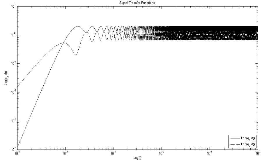
Figure 3: Averaged power transfer functions of the Doppler responses $x$ and $y$ to an ensemble of sinusoidal signals randomly polarized and uniformly distributed over the celestial sphere. The x-transfer function shows constructing interference at frequencies that are integer multiples of the inverse of the round-trip-light-time, $2L$, taken here to be equal to $5500$ seconds. The coupling of the $x$ data combination to such a stochastic ensemble of gravitational radiation is slightly stronger than that of the two-way $y$ response at frequencies larger than $5.0\times 10^{-4}$ Hz. At lower frequencies the transfer function of the $x$ combination decays more rapidly than that of $y$ as a consequence of being the difference of the two one-way measurements.

III.2 Noise Spectra

To compute the sensitivity of the combination $x$, and compare it against that of the two-way Doppler measurement, $y$, we need the one-sided power spectral densities of the main noise sources and their transfer functions to the observables $x$ and $y$. If we assume all the noise sources to be uncorrelated, from equations (5, 6) we can derive the following expressions for the two noise spectra $S_{x_{n}}$ and $S_{y_{n}}$

$$S_{x_{n}} = 4S_{C_{E}}+4S_{C_{S}}\cos^{2}(2\pi fL)+4S_{B}\sin^{2}(2\pi fL)+S_{A_{E}}+S_{A_{S}}+S_{EL_{E}}+S_{EL_{S}}\ ,$$ (9)

$$S_{y_{n}} = 4S_{C_{E}}\sin^{2}(2\pi fL)+4S_{T}\cos^{2}(2\pi fL)+4S_{B}+S_{A_{E}}+S_{A_{S}}+S_{EL_{E}}+S_{EL_{S}}+S_{TR}\ ,$$ (10)

where the meaning of the various terms appearing into Eqs. (9,10) is self-explanatory. We provide in the Appendix the expressions for the various noise spectra corresponding to a gravitational wave search performed with a spacecraft out to a distance of $5.5$ AU from Earth (as was during the first gravitational wave experiment with the CASSINI spacecraft), and equipped with an onboard microwave instrumentation similar to the one flown on CASSINI.

The gravitational wave sensitivity is the wave amplitude required to achieve a signal-to-noise ratio of $1$, and it can be computed as a function of Fourier frequency using the following expression Armstrong2006

$$\Sigma_{z}(f)\equiv\sqrt{\frac{S_{z_{n}}(f)\ B}{q_{z}(f)}}\ ,$$ (11)

where $z$ means either $x$ or $y$, and $B$ is the frequency bandwidth corresponding to a $40$ days integration time, the duration of the gravitational wave experiments performed with the CASSINI spacecraft Armstrong2006 .

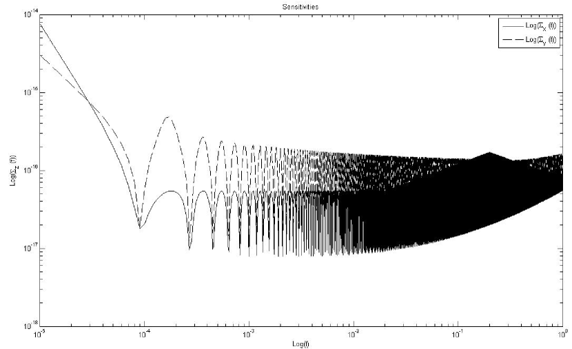
Figure 4: Sensitivities of the $x$ (solid-line) and $y$ (dash-line) Doppler responses to a randomly polarized and uniformly distributed stochastic ensemble of sinusoidal gravitational wave signals. The sensitivity is expressed as a function of the frequency and represents the equivalent sinusoidal strain required to produce a signal-to-noise ration of $1$. The spacecraft is assumed to be out to a distance of $5.5$ AU, and eighty percent tropospheric noise calibration is applied to the two-way Doppler data $y$ (dash-line). The two sensitivity curves reflect the noise spectral levels and shapes (given in the Appendix), their transfer functions to the observables $x$ and $y$ (Eqs. 9, 10), and the gravitational wave transfer functions shown in Fig. 3)

The main difference between the two observables $x$ and $y$ is of course in the absence in the $x$ combination of the joint disturbances from the troposphere and the mechanical vibration of the ground antenna (the random process denoted $T$ in Eq.(6)) and the presence (in $x$) of the spacecraft clock noise process. As onboard and ground microwave instrumentation have in recent years reached unprecedented frequency stabilities, $T$ has indeed become the major sensitivity limitation of two-way Doppler tracking searches for gravitational radiation Armstrong2006 . Since the effects from the troposphere can be mitigated by relying on simultaneous measurements performed by a radiometer located in the proximity of the tracking station, our sensitivity analysis reflects the assumption of being able to calibrate out eighty percent of the tropospheric effects from the $y$ observable (as demonstrated by the CASSINI experiments). Figure 4 shows the estimated sensitivity of the observable $x$ (continuous-line) formed out of the two one-way measurements, and compares it against that of the two-way measurement in which eighty percent of the tropospheric effects are calibrated out (dash-line). The $x$ combination displays the best sensitivity in the frequency band $10^{-4}-10^{-1}$ Hz, which is of most interest to gravitational wave search experiments. At higher frequencies, between about $10^{-1}-3.0\times 10^{-1}$ Hz, effects related to the locking of the atomic clock to its local oscillator introduce a small degradation in the $x$ sensitivity over that of the $y$ data. Also, at frequencies lower than $3.0\times 10^{-5}$ Hz, the $x$ combination shows a sensitivity worse than that of $y$ due to the cancellation of the signal in this low-frequency region.

As the two one-way Doppler measurements can be combined to synthesize the two-way measurement $y$ Piran_etal1986 ; Tinto1996 , one could argue that at these frequencies one could of course rely on the synthesized $y$ data to take advantage, if needed, of its better sensitivity in these two regions of the accessible frequency band. This observation suggests that it must be possible to identify a combination of the two one-way Doppler data that maximizes the sensitivity to gravitational waves in the entire band of interest.

III.3 Optimal Sensitivity

In order to derive the combination of the two one-way Doppler data that achieves optimal sensitivity, let us consider the following linear combination $\eta(f)$ of the Fourier transforms of $E(t)$ and $S(t)$

$$\eta(f)\equiv a_{1}(f,{\vec{\lambda}})\ {\widetilde{E}}(f)\ +\ a_{2}(f,{\vec{\lambda}})\ {\widetilde{S}}(f)\ ,$$ (12)

where the $\{a_{i}(f,\vec{\lambda})\}_{i=1,2}$ are arbitrary complex functions of the Fourier frequency $f$, and of a vector $\vec{\lambda}$ containing parameters characterizing the signal and the noises affecting the two Doppler data. For a given choice of the two functions $\{a_{i}\}_{i=1,2}$, $\eta$ gives a specific Doppler data combination, and our goal is therefore that of identifying, for a given signal, the two functions $\{a_{i}\}_{i=1,2}$ that maximize the signal-to-noise ratio Helstrom68 , $SNR_{\eta}^{2}$, of the combination $\eta$

$$SNR_{\eta}^{2}=\int_{f_{l}}^{f_{u}}\frac{|a_{1}\ {\widetilde{E}_{s}}+a_{2}\ {\widetilde{S}_{s}}|^{2}}{{\langle|a_{1}\ {\widetilde{E}_{n}}+a_{2}\ {\widetilde{S}_{n}}|^{2}\rangle}}\ df\ .$$ (13)

In equation (13) the subscripts $s$ and $n$ refer to the signal and the noise parts of (${\widetilde{E}},{\widetilde{S}}$) respectively, the angle brackets represent noise ensemble averages, and the interval of integration ($f_{l},f_{u}$) corresponds to the accessible frequency band.

The $SNR_{\eta}^{2}$ can be regarded as a functional over the space of the two complex functions $\{a_{i}\}_{i=1,2}$, and their expressions that maximize it can of course be derived by solving the associated set of Euler-Lagrange equations. The derivation of the expression of the optimal SNR, ${SNR_{\eta}^{2}}_{\rm opt}$, is long but straightforward, and it is equal to (see PTLA02 for details)

$${SNR_{\eta}^{2}}_{\rm opt.}=\int_{f_{l}}^{f_{u}}{\bf z}^{(s)*}_{i}\ ({\bf C}^{-1})_{ij}\ {\bf z}^{(s)}_{j}\ df\ .$$ (14)

In Eq. (14) the convention of sum over repeated indices is assumed, ${\bf z}^{(s)}$ is the vector of the signals, (${\widetilde{E_{s}}},{\widetilde{S_{s}}}$), and ${\bf C}$ is the hermitian, non-singular, correlation matrix of the vector random process ${\bf z}_{n}\equiv({\widetilde{E_{n}}},{\widetilde{S_{n}}})$

$$({\bf C})_{rt}\equiv\langle{\bf z}^{(n)}_{r}{\bf z}^{(n)*}_{t}\rangle\ .$$ (15)

Eq. (14) can now be used for estimating the sensitivity to an ensemble of sinusoidal gravitational wave signals randomly polarized and uniformly distributed over the celestial sphere. Figure 5 shows the estimated optimal sensitivity (solid-line) obtained by relying on the two one-way measurements, and again that of a two-way coherent tracking experiment (dash-line), in which all the parameters characterizing the experiment are as in Figure (4). Note how the sensitivity of the optimal combination is now consistently below that of the two-way measurement, and it coincides with that of the $x$ combination in most of the accessible frequency band.

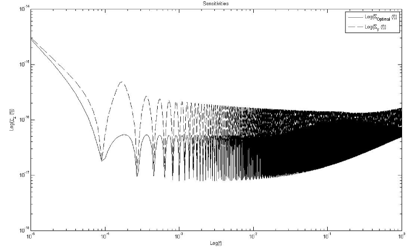
Figure 5: Sensitivity curves of the optimal combination (solid-line) and the two-way Doppler tracking data (dash-line). The noise parameters are equal to those used in figure 4. Note how the sensitivity of the optimal combination is now consistently below that of the two-way measurement.

IV Conclusions

We have discussed a method for significantly enhancing the sensitivity of Doppler tracking experiments aimed at the detection of gravitational waves. The main result of our analysis shows that by adding an atomic frequency standard and a digital receiver on board the spacecraft we can achieve a broad-band sensitivity of $2.0\times 10^{-17}$ in the milliHertz band. This sensitivity figure is obtained by completely removing the frequency fluctuations due to the interplanetary plasma. Our method relies on a properly chosen linear combination of the one-way Doppler data recorded on board with the data measured on the ground. It allows us to optimally suppress the frequency fluctuations due to the troposphere, ionosphere, and antenna mechanical and, for a spacecraft that is tracked for $40$ days out to $5.5$ AU, to reach a sensitivity that is about one order of magnitude better than that achievable by a state-of-the art two-way Doppler tracking search.

The expression of the optimal combination of the two one-way Doppler data can be used in all the classic tests of relativistic theory of gravity in which one-way and two-way spacecraft Doppler measurements are used as primary data sets. We will analyze the implications of the sensitivity improvements that this technique will provide for direct measurements of the gravitational red-shift, the second-order relativistic Doppler effect predicted by the theory of special relativity, searches for possible anisotropy in the velocity of light, measurements of the parameterized post-Newtonian parameters, and measurements of the deflection and time delay by the Sun in radio signals. This research is in progress, and will be the subject of a forthcoming investigation.

Appendix

IV.1 Noise sources and their spectra

This appendix provides a general description of the radio hardware needed for implementing the technique described in the main body of this paper, the corresponding one-sided power spectral densities of the frequency fluctuations introduced by these subsystems into the observables $E(t)$ and $S(t)$, and discusses the frequency fluctuations due to the Earth atmosphere. For a more comprehensive analysis on the radio hardware the reader is referred to Tinto1996 ; Tinto2000 ; Armstrong2006 ; Prestage_Weaver2007 ; Dick1990 ; RASSI_2008 , while a review on the propagation noises is given in Armstrong2006

The ground master clock and the frequency & timing distribution represent the overall contribution of the reference clock itself and the cabling system that takes the signal generated by the master clock to the antenna. This can be located several kilometers away from the site of the clock, implying that the need of a highly-stable cabling system is required. It has been shown at JPL that optical-fiber cables would not degrade significantly the frequency stability of the signal generated by the master clock. The corresponding one-sided power spectral density of the frequency fluctuations, introduced by these two noise sources, is equal to Tinto2000

$$S_{C_{E}}(f)=6.2\times[10^{-28}f+10^{-33}f^{-1}+10^{-30}]+1.3\times 10^{-28}f^{2}\ \ {\rm Hz}^{-1}\ .$$ (16)

The Ground and onboard Transmitters include all the frequency multipliers that are needed to generate the desired frequency of the transmitted radio signal, starting from the frequency provided by the clocks. It also accounts for the radio amplifier, and the extra phase delay changes occurring between the amplifier and the feed cone of the antennas. The noise due to the amplifiers is the dominant one, and it has been characterized in Tinto1996 . The one-sided power spectral densities of the frequency fluctuations are given by

$$S_{A_{E}}(f)+S_{A_{S}}(f)=2.3\times 10^{-28}+4.0\times 10^{-25}f\ \ {\rm Hz}^{-1}\ ,$$ (17)

The noises introduced by the Receiver at the ground station can be modeled as white phase fluctuations. The contribution to the overall noise budget from the receiver chain on the ground can be repartitioned into thermal noise (finiteness of the signal-to-noise ratio) and fluctuations introduced into the signal as it propagates through the cables and waveguides running from the feed of the antenna to the actual receiver. The effects of the latter noise source is nowadays minimized with the use of beam waveguide (BWG) antennas. These new antennas have become operational in the year 2004 at the NASA Deep Space Network three sites: in North America (Goldstone, California), Europe (Madrid, Spain), and Australia (Canberra).

Under the assumption of relying on a $34$ meter diameter beam waveguide antenna for receiving a coherent Ka-Band ($32$ GHz) signal transmitted by a spacecraft out a distance of $5.5$ AU, a ground system noise temperature of about $70$ degrees Kelvin, an onboard Ka-Band amplifier of $10$ W, and a spacecraft High Gain Antenna (HGA) with a diameter of about $4$ meters, we find the following one-sided power spectral density of the frequency fluctuations at Ka-Band Armstrong2006

$$S_{EL_{E}}(f)=6.3\times 10^{-27}\ f^{2}\ {\rm Hz}^{-1}\ .$$ (18)

The buffeting of the spacecraft will introduce unwanted frequency fluctuations in the one-way Doppler observable. Estimates of its magnitude have been given in Riley_etal1990 , and the one-sided power spectral density of the frequency fluctuations is given by the following expression

$$S_{B}(f)=5.0\ \times 10^{-42}\ f^{-3}\ +\ 1.0\ \times 10^{-31}\ {\rm Hz}^{-1}\ .$$ (19)

The noise introduced into the Doppler observable $y$ by the Earth Atmosphere and ionosphere, and by the scintillation of the interplanetary plasma, have been studied extensively in the literature AWE1979 ; Armstrong2006 ; Keihm1995 .

The scintillation introduced into the Doppler observables by the Atmosphere are independent of the microwave frequency at which the spacecraft is tracked. Since gravitational wave searches are performed in a band whose upper frequency cutoff is smaller than $1$ Hz (thermal noise at higher frequencies becomes unacceptably large), the one-sided power spectral density of the noise due to the atmosphere can be written as follows Linfield1998

$$S_{T}(f) = 2.8\ \times 10^{-28}\ f^{-2/5}\ \ {\rm Hz}^{-1}\ \ \ \ \ \ \ 10^{-5}\leq f\leq 10^{-2}\ \ {\rm Hz}$$ (20)

$$= 2.2\ \times 10^{-30}\ f^{-3}\ \ \ \ {\rm Hz}^{-1}\ \ \ \ \ \ \ 10^{-2}\leq f\leq 1\ \ \ \ \ \ \ {\rm Hz}\ .$$

The first term in the equation above accounts for the remaining effect of the atmosphere after eighty percent calibration is applied to the data with the use of a water vapor radiometer Armstrong2006 , while the second term accounts for the effect of aperture averaging, which causes a reduction in delay fluctuations on time scales less than the antenna wind speed crossing time ($1$ to $10$ seconds) Linfield1998 .

The Transponder entering into the $y$ measurement is responsible for keeping the phase coherence between the incoming and outgoing radio signals on the spacecraft. Its performance depends on the accuracy of tracking of the up-link signal by the phase locked loop, and the noise floor and non-linearities of its electronic components Riley_etal1990 . Frequency stability measurements of the Ka-Band ($32$ GHz) transponder flown onboard the CASSINI mission have resulted in the following one-sided power spectral density of the relative frequency fluctuations

$$S_{TR}(f)=1.6\times 10^{-26}\ f\ \ {\rm Hz}^{-1}\ .$$ (21)

The onboard clock provides the frequency and timing reference for the onboard radio instrumentation, and identifies the stability of the microwave signal transmitted to the ground. The space-qualified clock presently under realization at the Jet Propulsion Laboratory relies on a combined “interplay” between a local quartz oscillator and a trapped Hg ions clock. The frequency of the hyperfine transition made by the Hg ions is used for monitoring and correcting the frequency of the quartz oscillator. This steering process takes place on a typical time scale of about $10$ seconds, making then possible over longer time scale to significantly improve the stability of the resulting combined instrument. A frequency stability comparable to that of the Deep Space Network ground clocks has already been demonstrated with a prototype, showing an Allan standard deviation of a few parts in $10^{-15}$ at an integration time of a few thousand secondsPrestage_Weaver2007 ; Dick1990 . The corresponding one-sided power spectral density of the relative frequency fluctuations of such a clock is given by the following expression

$$S_{C_{S}} = 5.0\times 10^{-27}\ \ \ \ {\rm Hz}^{-1}\ \ \ \ \ \ \ \ \ \ \ 10^{-5}\leq f\leq 2.0\times 10^{-2}\ \ \ \ \ {\rm Hz}$$ (22)

$$= 2.5\times 10^{-25}f\ \ {\rm Hz}^{-1}\ \ \ \ \ \ 2.0\times 10^{-2}\leq f\leq 2.0\times 10^{-1}\ \ \ {\rm Hz}$$

$$= 10^{-26}f^{-1}\ \ \ \ \ \ \ {\rm Hz}^{-1}\ \ \ \ \ \ 2.0\times 10^{-1}\leq f\leq 1\ \ \ \ \ \ \ \ \ \ \ \ \ \ \ {\rm Hz}$$

The onboard digital receiver used in this method measures the amplitude and phase of the uplink signal and telemeters that information to the ground.

The frequency fluctuations of the receiver chain on board the spacecraft is estimated to be entirely due to thermal noise because of a simpler cabling system, and its performance being essentially identical to that of the ground receiver. By assuming again a $34$ meter diameter beam waveguide antenna transmitting with an $800$ W Ka-Band ($32$ GHz) amplifier to a spacecraft out to a distance of $5.5$ AU, equipped with a $4$ meter diameter (HGA), and a system noise temperature of $400$ Kelvin, we find the following one-sided power spectral density of the frequency fluctuations of the onboard electronics noise at Ka-Band Armstrong2006

$$S_{EL_{S}}(f)=7.2\times 10^{-28}\ f^{2}\ {\rm Hz}^{-1}\ .$$ (23)

References

References

- (1) A. Kliore, J.D. Anderson, J.W. Armstrong, S.W. Asmar, C.L. Hamilton, N.J. Rappaport, H.D. Wahlquist, R. Ambrosini, F.M. Flasar, R.G. French, L. Iess, E.A. Marouf, & A.F. Nagy, Space Sci. Rev., 115, 1–70, (2004).
- (2) R.F.C. Vessot. In: Proceedings of the XXVIIIth RENCONTRE DE MORIOND, eds. J. Tran Thanh Van, T. Damour, E. Hinds, and J. Wilkerson (Editions FRONTIERS), p.471-489, (1993).
- (3) B. Bertotti, L. Iess, & P. Tortora, Nature, 425, 374–376, (2003).
- (4) F.B. Estabrook and H.D. Wahlquist, Gen. Relativ. Gravit. 6, 439 (1975).
- (5) J.W. Armstrong, Living Reviews in Relativity 9, 1, (2006).
- (6) M. Tinto, Phys. Rev. D 53, 5354, (1996).
- (7) S.W. Asmar, J.W. Armstrong, L. Iess, & P. Tortora, Radio Sci., 40, (2005).
- (8) M. Tinto, Radio Sci. 37, 3, 1045, doi:10.1029/2001RS002473, (2002).
- (9) B. Bertotti, G. Comoretto, & L. Iess, Astron. Astrophys., 269, 608–616, (1993).
- (10) J.W. Armstrong, L. Iess, P. Tortora, & B. Bertotti, Astrophys. J., 599, 806–813, (2003).
- (11) J.A. Barnes, A.R. Chi, L.S. Cutler, D.J. Healey, D.B. Leeson, T.E. McGuniga, J.A. Mullen, W.L. Smith, R.L. Sydnor, R.F.C. Vessot, & G.M.R. Winkler, IEEE Trans. Instrum. Meas., 20, 105–120, (1971).
- (12) J.W. Armstrong, F.B. Estabrook, S.W. Asmar, L. Iess, & P. Tortora, Radio Sci., 43, RS3010, doi:10.1029/2007RS003766 28 June 2008.
- (13) J.D. Prestage, & G.L. Weaver. In: Proceedings of the IEEE, 95, 11, 2235-2247 (2007).
- (14) G.J. Dick, J.D. Prestage, C.A. Greenhall, & L. Maleki. In: Proceedings of the 22nd annual Precise Time and Time Interval (PTTI) Applications and Planning Meeting, The U.S. Naval Observatory publication. Available at: http://tycho.usno.navy.mil/ptti/1990/Vol
- (15) G. L. Tyler , I. R. Linscott, M. K. Bird, D. P. Hinson, D. F. Strobel, M. P tzold, M. E. Summers and K. Sivaramakrishnan, Space Sci. Rev., DOI 10.1007/s1214-007-9302-3, (2008).
- (16) The Radio Atmospheric Sounding and Scattering Instrument (RASSI), JPL proposal for constructing a flight radio science digital receiver. JPL internal publication (2008).
- (17) D. Kleppner, R.F.C. Vessot, & N.F. Ramsey, Astrophys. Space Sci., 6, 13-32, (1970).
- (18) R.F.C. Vessot, & M.W. Levine. In: A closeup of the Sun, Eds. M. Neugebauer, & R.W. Davis. JPL Publication 78-80, NASA (1978).
- (19) T. Piran, E. Reiter, W.G. Unruh, and R.F.C. Vessot, Phys. Rev. D, 34, 984, (1986).
- (20) J.W. Armstrong, R. Woo, and F.B. Estabrook, Ap.J., 230,570 (1979).
- (21) J.W. Armstrong, In: Proceedings of the NATO Advanced Research Workshop: Gravitational Wave Data Analysis, St. Nichols, Cardiff, Wales, 6 – 9 July 1987, NATO ASI Series C, vol. 253, 153–172, (Kluwer, Dordrecht, Netherlands; Boston, U.S.A., 1989), ed. B.F. Schutz.
- (22) M. Tinto, Open Loop Radio Science, Jet Propulsion Laboratory Publication - DSMS Telecommunications Link Design Handbook, 810-005, Rev. E, (2000). (http://eis.jpl.nasa.gov/deepspace/dsndocs/810-005/)
- (23) A.L. Riley, D. Antsos, J.W. Armstrong, P. Kinman, H.D. Wahlquist, B. Bertotti, G. Comoretto, B. Pernice, G. Carnicella, & R. Giordani, Cassini Ka-Band Precision Doppler and Enhanced Telecommunications System Study, Jet Propulsion Laboratory Report, Pasadena, California, January 22, 1990.
- (24) S.J. Keihm, TDA Progress Report, 42 - 122, 1-11, August 15, (1995).
- (25) R.P. Linfield, Radio Science, 33, 5 1353-1359, (1998).
- (26) C.W. Helström, Statistical Theory of Signal Detection, (Pergamon Press, London, 1968).
- (27) T.A. Prince, M. Tinto, S.L. Larson, and J.W. Armstrong Phys. Rev. D, 66, 122002, (2002).