Magnetization of two coupled rings

Abstract

We investigate the persistent currents and magnetization of a mesoscopic system consisting of two clean metallic rings sharing a single contact point in a magnetic field. Many novel features with respect to the single-ring geometry are underlined, including the explicit dependence of wavefunctions on the Aharonov-Bohm fluxes, the complex pattern of twofold and threefold degeneracies, the key rôle of length and flux commensurability, and in the case of commensurate ring lengths the occurrence of idle levels which do not carry any current. Spin-orbit interactions, induced by the electric fields of charged wires threading the rings, give rise to a peculiar version of the Aharonov-Casher effect where, unlike for a single ring, spin is not conserved. Remarkably enough, this can only be realized when the Aharonov-Bohm fluxes in both rings are neither integer nor half-integer multiples of the flux quantum.

,

1 Introduction

The orbital magnetic response of mesoscopic systems has been extensively studied in the last 25 years [1]. One of its manifestations is the occurrence of persistent currents and weak magnetism in small (sub-micron size) metallic rings threaded by a magnetic flux [2]. By ‘small’ one means that the circumference $L$ of the ring is much smaller than the phase coherence length $L_{\phi}$, and so quantum coherence is maintained throughout. This condition can be achieved at low enough temperatures. In a metallic ring disorder is very weak (as expressed in terms of the Ioffe-Regel condition $k_{F}\ell\gg 1$, with $k_{F}$ and $\ell$ being the Fermi momentum and the mean free path), and the currents persist for systems of a few microns in size [3], while for $k_{F}\ell\leq 1$ they decay exponentially with the system size. The magnetic response of metallic rings proved to be an important tool to study fundamental aspects of quantum mechanics, such as quantum coherence [4] and the Aharonov-Bohm (AB) effect [5, 6]. In systems exhibiting the AB effect, the magnetic flux appears as a pure Abelian U(1) gauge, in the sense that it only affects the phase of the wavefunction. Every observable quantity is therefore periodic in the magnetic flux (this is the Byers-Yang theorem [7]). Analogously, in the presence of a strong electric field (either internal or external), spin-orbit interactions give rise to the Aharonov-Casher (AC) effect [8, 9], which can be described as a pure non-Abelian SU(2) gauge.

Figure 1: The sample considered in this work consists of two clean wires modeled as ideal rings with lengths $L_{1}$ and $L_{2}$, areas $A_{1}$ and $A_{2}$, threaded by fluxes $\Phi_{1}$ and $\Phi_{2}$, touching at a contact point P.

In this work, motivated by these issues, we examine the relevance of the topology of the sample to its magnetic response. We investigate thoroughly a closed system composed of two (ideal) metallic rings sharing a single contact point P (see Figure 1). From a topological viewpoint, this sample has genus two, whereas a single ring has genus one. This difference turns out to enrich the physics in a rather non-trivial way, as already noticed in [10]. The present work includes a systematic study of the energy spectrum, persistent currents and magnetization of the sample shown in Figure 1, including their dependence on the ring lengths, on the magnetic fluxes, and on the number $N$ of electrons at zero temperature. The difference between the single and double-ring geometry is underlined throughout. The main novel features of the latter case are as follows. Wavefunctions generically depend on the fluxes. A rich pattern of twofold and threefold degeneracies is observed. As a consequence, the question whether a given level has a paramagnetic or diamagnetic response is more subtle than in the single-ring geometry. The commensurability of both ring lengths is a key issue. In the case of commensurate ring lengths, a finite fraction of the levels are ‘idle’, in the sense that their energies do not depend on the magnetic fluxes, so that these levels do not contribute to the persistent currents. The case of incommensurate ring lengths requires a special treatment, inspired from the theory of modulated incommensurate structures. As for the AC effect, the two-ring geometry allows one to study a novel feature which is absent in the single-ring geometry. Suppose that the AC effect is realized by threading a ring with a long straight wire with constant longitudinal charge density. In a single-ring geometry this construction implies that $s_{z}$, the spin component along the ring axis, is conserved, and so the problem decomposes into two independent ones, one for spin up and one for spin down. In the two-ring geometry, we can realize the AC effect as a pure gauge in an $s_{z}$ non-conserving system. Remarkably enough, this is possible only if the magnetic fluxes through both rings are non-trivial, i.e., neither integer nor half-integer multiples of the flux quantum. This kind of interplay between the AB and AC effects had not been noticed so far, to the best of our knowledge. Finally, the introduction of a non-Abelian SU(2) flux can also affect the sign of the sample’s magnetization, turning a diamagnetic to a paramagnetic response or vice versa.

In the following we elaborate and substantiate the issues presented above. Starting with the AB effect, the following topics are successively covered (section numbers in parentheses): the Hamiltonian and its characteristic equation (2), basic observables, including persistent currents and magnetization (3), various special cases of interest (4), twofold and threefold degeneracies (5), and the spectrum and observables for commensurate (6) and incommensurate (7) ring lengths. Then in Section 8 we examine the rôle of spin-orbit interactions and construct a Hamiltonian in terms of SU(2) fluxes leading to the AC effect. The energy levels and the magnetization are calculated in the special case of two equal rings, the emphasis being put on a novel AB-AC interference effect. A summary of our findings and a discussion are presented in Section 9, while two appendices are devoted to a reminder of the well-known case of a single ring (A), and to an extension of the analysis to three coupled rings (B).

2 The Hamiltonian and its characteristic equation

We consider a clean metallic sample in the form of two unequal rings touching at a contact point P, as shown in Figure 1. The rings are planar, but may otherwise assume arbitrary shapes. The rings have lengths $L_{1}$ and $L_{2}$ and areas $A_{1}$ and $A_{2}$. In the presence of a uniform transverse magnetic field $B$, they are therefore threaded by magnetic fluxes $\Phi_{1}=BA_{1}$ and $\Phi_{2}=BA_{2}$. In the case of circular rings, to be used in numerical illustrations of our results, we have $A_{1}=L_{1}^{2}/(4\pi)$ and $A_{2}=L_{2}^{2}/(4\pi)$. In order to compare both ring lengths, we introduce a variable $0<\omega<1$ so that

$$\frac{L_{1}}{L_{1}+L_{2}}=\omega,\quad\frac{L_{2}}{L_{1}+L_{2}}=1-\omega.$$ (2.1)

It will turn out that the system has different characteristics for commensurate lengths (rational $\omega$) and for incommensurate lengths (irrational $\omega$).

To write down the Hamiltonian, it is useful to employ reduced units ($\hbar=c=e=2m=1$), so that the flux quantum reads $\Phi_{0}=2\pi$. The spectrum and the observables are therefore $2\pi$-periodic in $\Phi_{1}$ and $\Phi_{2}$. We parametrize a point of the left ring by its curvilinear abscissa $0\leq s_{1}\leq L_{1}$, starting from the contact point P and oriented clockwise, and similarly a point of the right ring by $0\leq s_{2}\leq L_{2}$. Furthermore, we neglect spin degrees of freedom (except in Section 8). The one-body Hamiltonian of the system reads

$${\cal H}=(p_{1}-a_{1})^{2}+(p_{2}-a_{2})^{2},$$ (2.2)

with

$$p_{1}=-{\rm i}\,\frac{{\rm d}}{{\rm d}s_{1}},\quad p_{2}=-{\rm i}\,\frac{{\rm d}}{{\rm d}s_{2}},$$ (2.3)

whereas the tangential vector potentials $a_{1}$ and $a_{2}$ can be taken equal to

$$a_{1}=\frac{\Phi_{1}}{L_{1}},\quad a_{2}=\frac{\Phi_{2}}{L_{2}}.$$ (2.4)

A state $|\psi\rangle$ is described by a pair of wavefunctions $\{\psi^{(1)}(s_{1}),\;\psi^{(2)}(s_{2})\}$. The first term of the Hamiltonian ${\cal H}$ acts on the left component $\psi^{(1)}(s_{1})$, whereas the second term acts on the right component $\psi^{(2)}(s_{2})$. The behavior of the wavefunctions at the contact point P is in general described by a unitary junction $S$-matrix. In the present work we make the simplest choice, which corresponds to just requiring the continuity of the wavefunction:

$$\psi^{(1)}(0)=\psi^{(1)}(L_{1})=\psi^{(2)}(0)=\psi^{(2)}(L_{2})=\psi({\mathrm{P}}),$$ (2.5)

and the conservation of the current:

$$(p_{1}-a_{1})\psi^{(1)}(0)-(p_{1}-a_{1})\psi^{(1)}(L_{1})$$ (2.6)

$${\hskip-14.5pt}+(p_{2}-a_{2})\psi^{(2)}(0)-(p_{2}-a_{2})\psi^{(2)}(L_{2})=0.$$ (2.7)

Setting $E=q^{2}$ for the energy eigenvalue, we look for an eigenstate of ${\cal H}$ in the form

$$\matrix{\psi^{(1)}(s_{1})={\rm e}^{{\rm i}a_{1}s_{1}}(A_{1}{\rm e}^{{\rm i}qs_{1}}+B_{1}{\rm e}^{-{\rm i}qs_{1}}),\hfill\cr\psi^{(2)}(s_{2})={\rm e}^{{\rm i}a_{2}s_{2}}(A_{2}{\rm e}^{{\rm i}qs_{2}}+B_{2}{\rm e}^{-{\rm i}qs_{2}}).\hfill}$$ (2.8)

The condition (2.5) allows one to express these four amplitudes in terms of $\psi({\mathrm{P}})$ as

$$\matrix{A_{1}=\displaystyle{\displaystyle{\rm e}^{-{\rm i}\Phi_{1}}-{\rm e}^{-{\rm i}qL_{1}}\over\displaystyle 2{\rm i}\sin qL_{1}}\,\psi({\mathrm{P}}),\hfill&B_{1}=\displaystyle{\displaystyle{\rm e}^{{\rm i}qL_{1}}-{\rm e}^{-{\rm i}\Phi_{1}}\over\displaystyle 2{\rm i}\sin qL_{1}}\,\psi({\mathrm{P}}),\hfill\cr A_{2}=\displaystyle{\displaystyle{\rm e}^{-{\rm i}\Phi_{2}}-{\rm e}^{-{\rm i}qL_{2}}\over\displaystyle 2{\rm i}\sin qL_{2}}\,\psi({\mathrm{P}}),\hfill&B_{2}=\displaystyle{\displaystyle{\rm e}^{{\rm i}qL_{2}}-{\rm e}^{-{\rm i}\Phi_{2}}\over\displaystyle 2{\rm i}\sin qL_{2}}\,\psi({\mathrm{P}}).\hfill}$$ (2.9)

The condition (2.7) then yields the characteristic equation

$$D(q)=0,$$ (2.10)

where the characteristic function reads

$$D(q)=\sin q(L_{1}+L_{2})-\cos\Phi_{2}\,\sin qL_{1}-\cos\Phi_{1}\,\sin qL_{2}.$$ (2.11)

The eigenstates of the Hamiltonian correspond to the solutions $q_{n}\geq 0$ of (2.10), labeled by $n=1,2,\dots$ and ordered as $0\leq q_{1}\leq q_{2}\leq\dots$ The corresponding energy eigenvalues are $E_{n}=q_{n}^{2}$. In the special case where each ring is threaded by a quarter flux unit ($\Phi_{1}=\Phi_{2}=\pi/2$), we have $q_{n}=n\pi/(L_{1}+L_{2})$ (see (4.10)). In the general case, i.e., for arbitrary values of the fluxes, we set

$$q_{n}=\frac{n\pi+g_{n}}{L_{1}+L_{2}}\quad(n=1,2,\dots).$$ (2.12)

We will refer to $g_{n}$ as the modulation of the spectrum of eigenmomenta with respect to the linear behavior (4.10). This quantity will be shown in Section 7 to obey the bound

$$\left|g_{n}\right|\leq\pi.$$ (2.13)

The normalization of the wavefunction of the $n$th level reads

$$\langle\psi_{n}|\psi_{n}\rangle=\int_{0}^{L_{1}}\left|\psi_{n}^{(1)}(s_{1})\right|^{2}{\rm d}s_{1}+\int_{0}^{L_{2}}\left|\psi_{n}^{(2)}(s_{2})\right|^{2}{\rm d}s_{2}=\left|\psi_{n}({\mathrm{P}})\right|^{2}\Delta(q_{n}),$$ (2.14)

where

$$\Delta(q_{n})=L_{1}\,\frac{1-\cos\Phi_{1}\,\cos q_{n}L_{1}}{\sin^{2}q_{n}L_{1}}+L_{2}\,\frac{1-\cos\Phi_{2}\,\cos q_{n}L_{2}}{\sin^{2}q_{n}L_{2}},$$ (2.15)

hence

$$\psi_{n}({\mathrm{P}})=\Delta(q_{n})^{-1/2},$$ (2.16)

up to an irrelevant phase factor.

It is worth underlining a key difference between the present situation and that of a single ring, recalled in Appendix A. The gauge transformation employed in (2.8), while it locally eliminates the vector potential from the Schrödinger equation, does not lead to a Bloch-type boundary condition, at variance with (1.2). As a consequence, and in contrast with the single-ring wavefunction $\psi(s)$, the functions $\psi_{1}(s)$ and $\psi_{2}(s)$ given in (2.8) are not periodic in their respective arguments $s_{1}$ and $s_{2}$. The two-ring topology is indeed in marked difference with the single-ring one. Waves propagating in each ring are scattered at each passage at the contact point P. This multiple-scattering phenomenon destroys the periodicity of the plane waves characteristic of the single-ring problem. As a consequence, stationary states, as given by solutions of (2.10), bear in general a non-trivial dependence on both ring lengths $L_{1},L_{2}$ and on both fluxes $\Phi_{1},\Phi_{2}$. The periodicity of physical observables in the fluxes is however guaranteed by the Byers-Yang theorem, whose validity is independent of whether there is a Bloch analogue or not.

3 Persistent currents and magnetization

The contributions of the $n$th level to the persistent currents in each ring and to the magnetization read

$$I_{1,n}=-\displaystyle{\displaystyle\partial E_{n}\over\displaystyle\partial\Phi_{1}},\quad I_{2,n}=-\displaystyle{\displaystyle\partial E_{n}\over\displaystyle\partial\Phi_{2}},\quad M_{n}=-\displaystyle{\displaystyle\partial E_{n}\over\displaystyle\partial B}=A_{1}I_{1,n}+A_{2}I_{2,n}.$$ (3.1)

The persistent currents can be evaluated as follows. Considering $I_{1,n}$ for definiteness, we have

$$I_{1,n} = -\frac{1}{L_{1}}\,\frac{\partial E_{n}}{\partial a_{1}}=\frac{2}{L_{1}}\,\langle\psi_{n}|p_{1}-a_{1}|\psi_{n}\rangle$$ (3.2)

$$= \frac{2}{L_{1}}\,\int_{0}^{L_{1}}\psi_{n}^{{(1)}\star}(s_{1})\left(-{\rm i}\,\frac{{\rm d}}{{\rm d}s_{1}}-a_{1}\right)\psi_{n}^{(1)}(s_{1})\,{\rm d}s_{1}.$$ (3.3)

Using the expression (2.8) of the normalized wavefunction, together with (2.9), (2.15) and (2.16), we obtain after some algebra

$$I_{1,n}=\frac{2q_{n}}{L_{1}}\,Q_{1,n},\quad I_{2,n}=\frac{2q_{n}}{L_{2}}\,Q_{2,n},\quad M_{n}=2q_{n}\left(\frac{A_{1}Q_{1,n}}{L_{1}}+\frac{A_{2}Q_{2,n}}{L_{2}}\right),$$ (3.4)

where the dimensionless current amplitudes read

$$Q_{1,n}=-\frac{L_{1}\,\sin\Phi_{1}}{\sin q_{n}L_{1}\,\Delta(q_{n})},\quad Q_{2,n}=-\frac{L_{2}\,\sin\Phi_{2}}{\sin q_{n}L_{2}\,\Delta(q_{n})}.$$ (3.5)

An alternative approach consists in evaluating the currents from the spectrum. We have

$$I_{1,n}=-2q_{n}\,\frac{\partial q_{n}}{\partial\Phi_{1}}=2q_{n}\left(\frac{\partial D/\partial\Phi_{1}}{\partial D/\partial q}\right)_{q=q_{n}}=2q_{n}\,\frac{\sin\Phi_{1}\,\sin q_{n}L_{2}}{(\partial D/\partial q)_{q=q_{n}}}.$$ (3.6)

The current amplitudes can therefore be expressed as

$$Q_{1,n}=-L_{1}\,\frac{\partial q_{n}}{\partial\Phi_{1}}=-\omega\,\frac{\partial g_{n}}{\partial\Phi_{1}},\quad Q_{2,n}=-L_{2}\,\frac{\partial q_{n}}{\partial\Phi_{2}}=-(1-\omega)\,\frac{\partial g_{n}}{\partial\Phi_{2}}.$$ (3.7)

The following identity ensures that the results (3.4), (3.5) and (3.6), (3.7) are identical:

$$\left(\frac{\partial D}{\partial q}\right)_{q=q_{n}}=-\sin q_{n}L_{1}\,\sin q_{n}L_{2}\,\Delta(q_{n}).$$ (3.8)

For a zero-temperature system with $N$ electrons, the $N$ lowest energy states are occupied. The total energy and magnetization are therefore given by

$$E=\sum_{n=1}^{N}E_{n},\quad M=-\frac{\partial E}{\partial B}=\sum_{n=1}^{N}M_{n}.$$ (3.9)

Finally, explicit bounds on various quantities of interest can be derived by applying the inequality $\left|\langle\psi_{n}|{\cal O}|\psi_{n}\rangle\right|^{2}\leq\langle\psi_{n}|{\cal O}^{2}|\psi_{n}\rangle$ to the operators ${\cal O}_{1}=p_{1}-a_{1}$ and ${\cal O}_{2}=p_{2}-a_{2}$. The expression (3.3) implies that the persistent currents obey the bound

$$(L_{1}\,I_{1,n})^{2}+(L_{2}\,I_{2,n})^{2}\leq 4q_{n}^{2},$$ (3.10)

i.e.,

$$Q_{1,n}^{2}+Q_{2,n}^{2}\leq 1.$$ (3.11)

Furthermore, using (3.6) and (3.8), we can respectively recast (3.10) as

$$\Delta(q_{n})^{2}\geq\left(\frac{L_{1}\sin\Phi_{1}}{\sin q_{n}L_{1}}\right)^{2}+\left(\frac{L_{2}\sin\Phi_{2}}{\sin q_{n}L_{2}}\right)^{2}$$ (3.12)

and

$$\left(\frac{\partial D}{\partial q}\right)^{2}_{q=q_{n}}\geq(L_{1}\sin\Phi_{1}\,\sin q_{n}L_{2})^{2}+(L_{2}\sin\Phi_{2}\,\sin q_{n}L_{1})^{2}.$$ (3.13)

4 Special cases of interest

4.1 No magnetic fluxes

We consider first the problem in the absence of fluxes: $\Phi_{1}=\Phi_{2}=0\ {\rm(mod.}\ 2\pi)$. The characteristic function (2.11) factors as

$$D(q)=-4\,\sin\frac{q(L_{1}+L_{2})}{2}\,\sin\frac{qL_{1}}{2}\,\sin\frac{qL_{2}}{2}.$$ (4.1)

The spectrum therefore consists of the following three sectors, in correspondence with the factors of the above expression.

• Bilateral states. These states correspond to $\sin q(L_{1}+L_{2})/2=0$, hence

  $$q=\frac{b\pi}{L_{1}+L_{2}}\quad(b=0,2,4,\dots),$$ (4.2)

  with ‘$b$’ for bilateral. The corresponding wavefunctions are standing waves living on the whole system:

  $$\matrix{\psi^{(1)}(s_{1})=\psi({\mathrm{P}})\,\displaystyle{\displaystyle\cos qs_{1}+\cos q(L_{1}-s_{1})\over\displaystyle 1+\cos qL_{1}},\hfill\cr\psi^{(2)}(s_{2})=\psi({\mathrm{P}})\,\displaystyle{\displaystyle\cos qs_{2}+\cos q(L_{2}-s_{2})\over\displaystyle 1+\cos qL_{1}}.\hfill}$$ (4.3)

• Left states. These states correspond to $\sin qL_{1}/2=0$, hence

  $$q=\frac{l\pi}{L_{1}}\quad(l=2,4,6,\dots),$$ (4.4)

  with ‘$l$’ for left. The corresponding wavefunctions are standing waves living on the left ring, whose amplitude vanishes at the contact point:

  $$\psi^{(1)}(s_{1})\sim\sin qs_{1},\quad\psi^{(2)}(s_{2})=0.$$ (4.5)

• Right states. These states correspond to $\sin qL_{2}/2=0$, hence

  $$q=\frac{r\pi}{L_{2}}\quad(r=2,4,6,\dots),$$ (4.6)

  with ‘$r$’ for right. The corresponding wavefunctions are standing waves living on the right ring, whose amplitude vanishes at the contact point:

  $$\psi^{(1)}(s_{1})=0,\quad\psi^{(2)}(s_{2})\sim\sin qs_{2}.$$ (4.7)

The ground-state energy, obtained by setting $b=0$ in (4.2), vanishes. The modulation introduced in (2.12) reads $g_{1}=-\pi$, which saturates the bound (2.13). The corresponding ground-state wavefunction is uniform: $\psi^{(1)}(s_{1})=\psi^{(2)}(s_{2})=\psi({\mathrm{P}})$.

For small fluxes, we have

$$E_{1}\approx\frac{1}{L_{1}+L_{2}}\left(\frac{\Phi_{1}^{2}}{L_{1}}+\frac{\Phi_{2}^{2}}{L_{2}}\right),$$ (4.8)

so that the ground state is always diamagnetic. As far as excited states are concerned, the results (4.2), (4.4) and (4.6) respectively become

$$\matrix{q(L_{1}+L_{2})\approx b\pi+\displaystyle{\displaystyle\Phi_{1}^{2}-\Phi_{2}^{2}\over\displaystyle 2}\,\cot b\pi\omega,\hfill\cr qL_{1}\approx l\pi+\displaystyle{\displaystyle\Phi_{1}^{2}\over\displaystyle 2}\,\cot\displaystyle{\displaystyle l\pi\over\displaystyle\omega},\hfill\cr qL_{2}\approx r\pi+\displaystyle{\displaystyle\Phi_{2}^{2}\over\displaystyle 2}\,\cot\displaystyle{\displaystyle r\pi\over\displaystyle 1-\omega}.\hfill}$$ (4.9)

These results show that there is no general rule to predict whether a given (left or right) state is paramagnetic or diamagnetic. Bilateral states are always hybrid (one paramagnetic ring and one diamagnetic one).

The only degeneracies between the three interlaced spectra (4.2), (4.4) and (4.6) are the threefold ones taking place in the commensurate case at $qa=\theta=\pi\nu$, where $\nu=2\mu=2,4,6,\dots$ is an even integer. With the notations of Section 6, these momentum values correspond to $b=\mu m$, $l=\mu m_{1}$ and $r=\mu m_{2}$. The quadratic terms in (4.9) diverge. This is in agreement with the fact that near a degeneracy the energy eigenvalues vary linearly with the fluxes, rather than quadratically (see Section 5 for more details).

4.2 Integer or half-integer fluxes

Whenever each flux is either integer or half-integer (i.e., an integer or a half-integer multiple of the flux quantum $\Phi_{0}=2\pi$), the spectrum of the system still consists of the above three types of states (bilateral, left and right). The corresponding momenta are still given by (4.2), (4.4) and (4.6). Table 1 lists the characteristics of the spectrum in the four different cases, corresponding to $\Phi_{1}=0$ or $\pi\ {\rm(mod.}\ 2\pi)$ and $\Phi_{2}=0$ or $\pi\ {\rm(mod.}\ 2\pi)$.

$\Phi_{1}$	$\Phi_{2}$	$D(q)$	$b$	$l$	$r$
$0$	$0$	$-4\,\sin\displaystyle{\displaystyle q(L_{1}+L_{2})\over\displaystyle 2}\,\sin\displaystyle{\displaystyle qL_{1}\over\displaystyle 2}\,\sin\displaystyle{\displaystyle qL_{2}\over\displaystyle 2}$	$0,2,4,\dots$	$2,4,6,\dots$	$2,4,6,\dots$
$0$	$\pi$	$4\,\cos\displaystyle{\displaystyle q(L_{1}+L_{2})\over\displaystyle 2}\,\sin\displaystyle{\displaystyle qL_{1}\over\displaystyle 2}\,\cos\displaystyle{\displaystyle qL_{2}\over\displaystyle 2}$	$1,3,5,\dots$	$2,4,6,\dots$	$1,3,5,\dots$
$\pi$	$0$	$4\,\cos\displaystyle{\displaystyle q(L_{1}+L_{2})\over\displaystyle 2}\,\cos\displaystyle{\displaystyle qL_{1}\over\displaystyle 2}\,\sin\displaystyle{\displaystyle qL_{2}\over\displaystyle 2}$	$1,3,5,\dots$	$1,3,5,\dots$	$2,4,6,\dots$
$\pi$	$\pi$	$4\,\sin\displaystyle{\displaystyle q(L_{1}+L_{2})\over\displaystyle 2}\,\cos\displaystyle{\displaystyle qL_{1}\over\displaystyle 2}\,\cos\displaystyle{\displaystyle qL_{2}\over\displaystyle 2}$	$2,4,6,\dots$	$1,3,5,\dots$	$1,3,5,\dots$

Table 1: Characteristics of the system for the four cases with integer or half-integer fluxes: factorized form of the characteristic function $D(q)$; integers $b$, $l$ and $r$ entering the spectra (4.2), (4.4) and (4.6), respectively corresponding to bilateral, left and right states.

Left and right states are met in a more general setting. More precisely, left states with even (resp. odd) $l$ exist as soon as $\Phi_{1}=0$ (resp. $\Phi_{1}=\pi\ {\rm(mod.}\ 2\pi))$, irrespective of $\Phi_{2}$, whereas right states with even (resp. odd) $r$ exist as soon as $\Phi_{2}=0$ (resp. $\Phi_{2}=\pi\ {\rm(mod.}\ 2\pi))$, irrespective of $\Phi_{1}$.

4.3 Quarter-integer fluxes

The situation where each ring is threaded by a quarter flux unit ($\Phi_{1}=\Phi_{2}=\pi/2$) is also a special case of interest. In this case, the characteristic function boils down to $D(q)=\sin q(L_{1}+L_{2})$. The momenta therefore have the linear dependence

$$q_{n}=\frac{n\pi}{L_{1}+L_{2}}\quad(n=1,2,\dots).$$ (4.10)

In spite of the simplicity of the spectrum, the current amplitudes have the following non-trivial expressions:

$$Q_{1,n}=-\omega\sin n\pi\omega,\quad Q_{2,n}=(-1)^{n}(1-\omega)\sin n\pi\omega.$$ (4.11)

These quantities obey $\left|Q_{1,n}\right|\leq\omega$, $\left|Q_{2,n}\right|\leq 1-\omega$, and $\left|Q_{1,n}\right|+\left|Q_{2,n}\right|\leq 1$, the latter bound being more stringent than the general one (3.11). The currents in both rings therefore have the same sign (resp. opposite signs) whenever the level number $n$ is odd (resp. even).

Using (3.7), the result (4.11) can be recast as follows. If the fluxes are close to a quarter flux quantum, setting $\Phi_{1}=\pi/2+\delta\Phi_{1}$, $\Phi_{2}=\pi/2+\delta\Phi_{2}$, the modulation $g_{n}$ introduced in (2.12) reads, to first order in $\delta\Phi_{1}$ and $\delta\Phi_{2}$,

$$g_{n}\approx\sin n\pi\omega\times\left\{\matrix{\delta\Phi_{1}-\delta\Phi_{2}&\hbox{for}&n\;\hbox{even},\cr\delta\Phi_{1}+\delta\Phi_{2}&\hbox{for}&n\;\hbox{odd}.\hfill}\right.$$ (4.12)

5 Degeneracies

A degeneracy manifests itself as a multiple (i.e., at least double) root of the characteristic equation (2.10), i.e., as a simultaneous root of $D(q)=0$ and $\partial D/\partial q=0$. The bound (3.13) shows that the system has no accidental degeneracy. A degeneracy may indeed only take place when both products $\sin\Phi_{1}\,\sin qL_{2}$ and $\sin\Phi_{2}\,\sin qL_{1}$ vanish simultaneously, i.e., when at least one factor of each product vanishes. It can be checked that there are only two types of degeneracies, to be successively investigated hereafter.

5.1 Twofold degeneracies

Twofold degeneracies occur when either $\sin qL_{1}=\sin\Phi_{1}=0$ (but $\sin qL_{2}\neq 0$) or $\sin qL_{2}=\sin\Phi_{2}=0$ (but $\sin qL_{1}\neq 0$). These two instances will be respectively referred to as left and right degeneracies, for a reason that will become clear in a while.

Consider the first instance for definiteness. This is a left degeneracy, as the state to become twofold degenerate is a left state, in the sense of Section 4.1. We have $\cos qL_{1}=\cos\Phi_{1}=(-1)^{l}$, with the notation (4.4), so that

$$\frac{\partial D}{\partial q}=(-1)^{l}L_{1}(\cos qL_{2}-\cos\Phi_{2}).$$ (5.1)

The conditions for a twofold degeneracy are therefore

$$\sin qL_{1}=\sin\Phi_{1}=0,\quad\cos qL_{2}=\cos\Phi_{2}.$$ (5.2)

At the degeneracy the momentum is $q=l\pi/L_{1}$, whereas the fluxes read $\Phi_{1}=(2j+l)\pi$ and $\Phi_{2}=(2k+\varepsilon lL_{2}/L_{1})\pi$, where $\varepsilon=\pm 1$, whereas $j$ and $k$ are integers. For circular rings (more generally, for rings with similar shapes), we have $\Phi_{2}/\Phi_{1}=A_{2}/A_{1}=(L_{2}/L_{1})^{2}=((1-\omega)/\omega)^{2}$. This condition relates $\omega$ to $\varepsilon$, $j$ and $k$ as follows:

$$\matrix{\varepsilon=+1:\hfill&2(j-k+l)\omega^{2}-(4j+3l)\omega+2j+l=0,\hfill\cr\varepsilon=-1:\hfill&2(j-k)\omega^{2}-(4j+l)\omega+2j+l=0.\hfill}$$ (5.3)

The system may therefore have twofold degeneracies both in the commensurate case ($\omega$ rational) and in the incommensurate case provided $\omega$ is a quadratic number, obeying an equation of the form

$$I\omega^{2}+J\omega+K=0,$$ (5.4)

where $I$, $J$ and $K$ are integers.

In order to explore the vicinity of the degeneracy, we set

$$q=\frac{l\pi}{L_{1}}+\eta,\quad\Phi_{1}=l\pi+\delta\Phi_{1},\quad\Phi_{2}=\frac{l\pi L_{2}}{L_{1}}+\delta\Phi_{2}.$$ (5.5)

By expanding the characteristic equation (2.10) to second order in $\eta$, $\delta\Phi_{1}$ and $\delta\Phi_{2}$, we obtain the reduced equation

$$L_{1}(L_{1}+2L_{2})\eta^{2}-2L_{1}\delta\Phi_{2}\,\eta-\delta\Phi_{1}^{2}=0.$$ (5.6)

The momenta of the two nearly degenerate states are therefore given by

$$\eta_{\pm}=\frac{L_{1}\delta\Phi_{2}\pm W_{2}}{L_{1}(L_{1}+2L_{2})},$$ (5.7)

with the definition

$$W_{2}=\left(L_{1}(L_{1}+2L_{2})\delta\Phi_{1}^{2}+L_{1}^{2}\delta\Phi_{2}^{2}\right)^{1/2}.$$ (5.8)

The momenta shifts $\eta_{\pm}$ vanish linearly with the distance to the degeneracy in the $(\delta\Phi_{1},\delta\Phi_{2})$ plane. The corresponding amplitudes of the persistent currents read

$$Q_{1,\pm}=\mp\frac{L_{1}\delta\Phi_{1}}{W_{2}},\quad Q_{2,\pm}=\frac{L_{2}}{L_{1}+2L_{2}}\left(1\pm\frac{L_{1}\delta\Phi_{2}}{W_{2}}\right).$$ (5.9)

These amplitudes therefore remain of order unity, and they depend on the direction in the $(\delta\Phi_{1},\delta\Phi_{2})$ plane along which the degeneracy point is approached. As this direction is varied, the amplitudes describe an ellipse:

$$(1-\omega)^{2}Q_{1}^{2}+\omega(2-\omega)Q_{2}^{2}-2\omega(1-\omega)Q_{2}=0.$$ (5.10)

5.2 Threefold degeneracies

We have noticed at the end of Section 4.1 that the spectrum has threefold degeneracies in the absence of fluxes in the commensurate case at $qa=\theta=\pi\nu$, where $\nu=2\mu=2,4,\dots$ is an even integer, with the notations of Section 6.

More generally, there are threefold degeneracies at all the energies of the idle states, given by (6.4), i.e., $qa=\theta=\pi\nu$, with $\nu=1,2,\dots$ Consider indeed one of these energies. We have

$$\frac{\partial D}{\partial q}=a\varepsilon_{1}\varepsilon_{2}(m_{1}(1-\varepsilon_{2}\,\cos\Phi_{2})+m_{2}(1-\varepsilon_{1}\,\cos\Phi_{1})),$$ (5.11)

with the notations (6.6). The conditions for a threefold degeneracy are therefore

$$\cos\Phi_{1}=\varepsilon_{1},\quad\cos\Phi_{2}=\varepsilon_{2}.$$ (5.12)

Right at the degeneracy, the fluxes therefore read $\Phi_{1}=\pi\nu m_{1}$ and $\Phi_{2}=\pi\nu m_{2}\ {\rm(mod.}\ 2\pi)$. The situation in the absence of fluxes is recovered when $\nu$ is even. If $\nu$ is odd, at least one of the fluxes is a half integer, because at least one of the integers $m_{1}$, $m_{2}$ is odd.

In order to explore the vicinity of the degeneracy, we set

$$\theta=\nu\pi+\eta,\quad\Phi_{1}=\pi\nu m_{1}+\delta\Phi_{1},\quad\Phi_{2}=\pi\nu m_{2}+\delta\Phi_{2}.$$ (5.13)

By expanding the characteristic equation (2.10) to third order in $\eta$, and to second order in $\delta\Phi_{1}$ and $\delta\Phi_{2}$, we find three solutions: the idle state at $\eta=0$, and two symmetrically shifted active states at $\eta_{\pm}=\pm W_{3}$, with

$$W_{3}=\left(\frac{m_{2}\delta\Phi_{1}^{2}+m_{1}\delta\Phi_{2}^{2}}{m_{1}m_{2}(m_{1}+m_{2})}\right)^{1/2}.$$ (5.14)

The momentum shift $W_{3}$ again vanishes linearly with the distance to the degeneracy in the ($\delta\Phi_{1},\delta\Phi_{2}$) plane. The corresponding amplitudes of the persistent currents read

$$Q_{1,\pm}=\mp\frac{\delta\Phi_{1}}{(m_{1}+m_{2})W_{3}},\quad Q_{2,\pm}=\mp\frac{\delta\Phi_{2}}{(m_{1}+m_{2})W_{3}}.$$ (5.15)

Here again, these amplitudes remain of order unity and depend on the direction in the ($\delta\Phi_{1},\delta\Phi_{2}$) plane along which the degeneracy point is approached. As this direction is varied, the amplitudes describe an ellipse:

$$(1-\omega)Q_{1}^{2}+\omega Q_{2}^{2}-\omega(1-\omega)=0.$$ (5.16)

6 Commensurate ring lengths

We now turn to the situation where the ring lengths $L_{1}$ and $L_{2}$ are commensurate. One of the peculiar features of this situation is the existence of threefold degeneracies, already investigated in Section 5.2.

In the commensurate situation, both ring lengths are multiples of the same fundamental length $a$:

$$L_{1}=m_{1}a,\quad L_{2}=m_{2}a,$$ (6.1)

where the integers $m_{1}\geq 1$ and $m_{2}\geq 1$ are relatively prime. Setting $m=m_{1}+m_{2}\geq 2$, the variable $\omega$ takes the rational value $\omega=m_{1}/m$. For circular commensurate rings, the fluxes read $\Phi_{1}=m_{1}^{2}\,Ba^{2}/(4\pi)$, $\Phi_{2}=m_{2}^{2}\,Ba^{2}/(4\pi)$, so that the magnetization is periodic in the magnetic field $B$, with period $B_{0}=8\pi^{2}/a^{2}$.

6.1 Spectrum

Introducing the reduced momentum

$$\theta=qa,$$ (6.2)

the characteristic function becomes

$$D(\theta)=\sin m\theta-\cos\Phi_{2}\,\sin m_{1}\theta-\cos\Phi_{1}\,\sin m_{2}\theta.$$ (6.3)

The spectrum of the system is $2\pi$-periodic in $\theta$. It consists of two types of states.

• Idle states. They correspond to the trivial solutions of the characteristic equation:

  $$\theta=\pi\nu\quad(\nu=1,2,\dots).$$ (6.4)

  These states carry no current, as their energy is independent of the fluxes. The corresponding wavefunctions do however depend on the fluxes. We have indeed

  $$\matrix{\psi^{(1)}(s_{1})\sim({\rm e}^{-{\rm i}\Phi_{2}/2}-\varepsilon_{2}\,{\rm e}^{{\rm i}\Phi_{2}/2}){\rm e}^{{\rm i}a_{1}s_{1}}\sin qs_{1},\cr\psi^{(2)}(s_{2})\sim(\varepsilon_{1}\,{\rm e}^{{\rm i}\Phi_{1}/2}-{\rm e}^{-{\rm i}\Phi_{1}/2}){\rm e}^{{\rm i}a_{2}s_{2}}\sin qs_{2},}$$ (6.5)

  with

  $$\varepsilon_{1}={\rm e}^{{\rm i}qL_{1}}=(-1)^{\nu m_{1}},\quad\varepsilon_{2}={\rm e}^{{\rm i}qL_{2}}=(-1)^{\nu m_{2}}.$$ (6.6)

  Idle states become threefold degenerate for integer or half-integer values of the fluxes such that the condition (5.12) is fulfilled.

• Active states. These states, corresponding to the other solutions of the characteristic equation $D(\theta)=0$, carry non-zero persistent currents in general.

  Setting $c=\cos\theta$, we have the identity $\sin m\theta=\sin\theta\,U_{m-1}(c)$, where $U_{n}(c)$ is the $n$th Tchebyshev polynomial of the second kind, whose degree is $n$. Focusing onto active states, the characteristic equation therefore reads

  $$U_{m-1}(c)-\cos\Phi_{2}\,U_{m_{1}-1}(c)-\cos\Phi_{1}\,U_{m_{2}-1}(c)=0.$$ (6.7)

  This equation has $m-1$ solutions $c_{(k)}$ ($k=1,\dots,m-1$). We write these solutions as $c_{(k)}=\cos\theta_{(k)}$, with $0\leq\theta_{(k)}\leq\pi$, ordered as

  $$0\leq\theta_{(1)}\leq\dots\leq\theta_{(m-1)}\leq\pi.$$ (6.8)

  Threefold degeneracies correspond to the limiting situations $\theta_{(1)}=0$ or $\theta_{(m-1)}=\pi$, whereas twofold ones can take place anywhere along the sequence of $\theta_{(k)}$’s.

To sum up, in each period of the spectrum of length $2\pi$ in the variable $\theta=qa$, there are $2(m-1)$ active levels and 2 idle ones, i.e., a total of $2m$ states. The modulation and the current amplitudes associated with the states at $\theta=\theta_{(k)}$ ($k=1,\dots,m-1$) read

$$g_{k}=m\theta_{(k)}-k\pi,\quad Q_{1,k}=-m_{1}\,\frac{\partial\theta_{(k)}}{\partial\Phi_{1}},\quad Q_{2,k}=-m_{2}\,\frac{\partial\theta_{(k)}}{\partial\Phi_{2}},$$ (6.9)

whereas those associated with the states at $\theta=2\pi-\theta_{(i)}$,

$$g_{2m-k}=k\pi-m\theta_{(k)},\quad Q_{1,2m-k}=m_{1}\,\frac{\partial\theta_{(k)}}{\partial\Phi_{1}},\quad Q_{2,2m-k}=m_{2}\,\frac{\partial\theta_{(k)}}{\partial\Phi_{2}},$$ (6.10)

are the opposites of the first expressions. The bound (2.13) implies

$$(k-1)\pi\leq m\theta_{(k)}\leq(k+1)\pi\quad(k=1,\dots,m-1).$$ (6.11)

Modulation and current amplitudes then repeat themselves periodically, with period $2m$. The main characteristics of the states in the first period are listed in Table 2.

$n$	1	$\dots$	$m-1$	$m$	$m+1$	$\dots$	$2m-1$	$2m$
$\theta$	$\theta_{(1)}$	$\dots$	$\theta_{(m-1)}$	$\pi$	$2\pi-\theta_{(m-1)}$	$\dots$	$2\pi-\theta_{(1)}$	$2\pi$
type	A	$\dots$	A	I	A	$\dots$	A	I
$g_{n}$	$g_{1}$	$\dots$	$g_{m-1}$	0	$-g_{m-1}$	$\dots$	$-g_{1}$	0
$Q_{1,n}$	$Q_{1,1}$	$\dots$	$Q_{1,m-1}$	0	$-Q_{1,m-1}$	$\dots$	$-Q_{1,1}$	0
$Q_{2,n}$	$Q_{2,1}$	$\dots$	$Q_{2,m-1}$	0	$-Q_{2,m-1}$	$\dots$	$-Q_{2,1}$	0

Table 2: The first $2m$ states of the system in the commensurate case, corresponding to the first period of the spectrum in the variable $\theta=qa$. For each column, corresponding to a state, the table gives the level number $n$, the angle $\theta$, the type of state (‘I’ for idle or ‘A’ for active), the modulation and the current amplitudes.

6.2 Rings with equal lengths

The case where both rings have equal lengths is the simplest of all the commensurate situations. We have $m_{1}=m_{2}=1$, $m=2$, $\omega=1/2$ and $a=L=L_{1}=L_{2}$. The characteristic equation (6.7) has a single solution:

$$c_{(1)}=\cos\theta_{(1)}=\frac{\cos\Phi_{1}+\cos\Phi_{2}}{2}.$$ (6.12)

Idle states ($n=2p$) and active states ($n=2p-1$) alternate along the spectrum:

$$q_{2p}=\frac{p\pi}{L},\quad q_{2p-1}=\frac{(2p-1)\pi+(-1)^{p-1}g_{1}}{2L}.$$ (6.13)

The modulation and the current amplitudes of the lowest active state ($n=2p-1=1$, i.e., $p=1$) read

$$g_{1}=2\theta_{(1)}-\pi,\quad Q_{1,1}=-\frac{\sin\Phi_{1}}{2\sin\theta_{(1)}},\quad Q_{2,1}=-\frac{\sin\Phi_{2}}{2\sin\theta_{(1)}}.$$ (6.14)

In the case of two equal circular rings, the above predictions can be made fully explicit. We have $\Phi_{1}=\Phi_{2}=\Phi=BL^{2}/(4\pi)$. Symmetry considerations allow us to restrict ourselves to $0\leq\Phi\leq\pi$, so that $\theta_{(1)}=\Phi$, $g_{1}=2\Phi-\pi$ and $Q_{1,1}=Q_{2,1}=-1/2$. Hence, using (3.4), the contribution of any odd state ($n=2p-1$) to the magnetization reads

$$M_{2p-1}=(-1)^{p}\,\frac{2p-1}{4}+\frac{\pi-2\Phi}{4\pi}.$$ (6.15)

Inserting this formula into (3.9), we obtain the expression of the magnetization of a system with $N$ electrons at zero temperature. This expression, given in Table 3, depends on $N\ {\rm(mod.}\ 4)$. The corresponding result for a single circular ring, given by (1.6), (1.7), is also listed in the Table for comparison (the latter depends on the sign of $N$, i.e., on $N\ {\rm(mod.}\ 2)$).

$N\ {\rm(mod.}\ 4)$	$M$ (two equal rings)	$M$ (one single ring)
0	$N(\pi-\Phi)/(4\pi)$	$N(\pi-\Phi)/(2\pi)$
1	$-(N+1)\Phi/(4\pi)$	$-N\Phi/(2\pi)$
2	$-N\Phi/(4\pi)$	$N(\pi-\Phi)/(2\pi)$
3	$(N+1)(\pi-\Phi)/(4\pi)$	$-N\Phi/(2\pi)$

Table 3: Expression of the magnetization $M$ of a system with $N$ electrons at zero temperature, as a function of the flux $\Phi$ in the range $0\leq\Phi\leq\pi$, for two equal circular rings and for a single circular ring.

6.3 Magnetization

The simple linear dependence of the magnetization on the magnetic field in the range $0\leq\Phi\leq\pi$, observed in Table 3, is a peculiarity of the cases considered there, namely one single circular ring or two equal ones.

In all the other cases of commensurate circular rings, the curve $M(B)$ is non-trivial. This is illustrated in Figure 2, showing plots of the magnetization over one period, against $\Phi_{1}/(2\pi)=B/B_{0}=BL_{1}^{2}/(8\pi^{2})$, for $L_{2}=L_{1}$ (left) and $L_{2}=2L_{1}$ (right). The latter example ($m_{1}=1$, $m_{2}=2$, $m=3$) is generic of the commensurate case, except that the characteristic equation (6.7) is of degree two in $c$ and can therefore be solved analytically. We thus obtain

$$\matrix{c_{(1)}=\cos\theta_{(1)}=\displaystyle{\displaystyle 1\over\displaystyle 4}\left(\cos\Phi_{1}+(4+4\cos\Phi_{2}+\cos^{2}\Phi_{1})^{1/2}\right),\cr c_{(2)}=\cos\theta_{(2)}=\displaystyle{\displaystyle 1\over\displaystyle 4}\left(\cos\Phi_{1}-(4+4\cos\Phi_{2}+\cos^{2}\Phi_{1})^{1/2}\right).}$$ (6.16)

The currents and the magnetization then follow from (6.9), (6.10) and (3.4), (3.9).

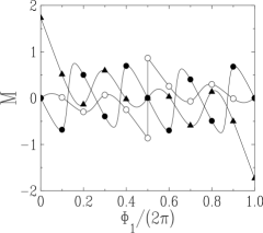
Figure 2: Plots of the magnetization $M$ over one period, against $\Phi_{1}/(2\pi)=BL_{1}^{2}/(8\pi^{2})$, for commensurate circular rings with $L_{2}=L_{1}$ (left) and $L_{2}=2L_{1}$ (right), for $N=3$ (empty circles), $N=4$ (full circles) and $N=5$ (full triangles). Data for $N=3$ and $N=4$ coincide on the left plot, as $n=4$ is an idle state.

7 Incommensurate ring lengths

We now turn to the situation where the ring lengths $L_{1}$ and $L_{2}$ are incommensurate, i.e., the variable $\omega$ is irrational.

The key quantity is again the modulation $g_{n}$ of the spectrum. In the commensurate case, i.e., for a rational $\omega=m_{1}/m$, $g_{n}$ has been shown to be periodic in $n$, with period $2m$. In the present incommensurate case, $g_{n}$ is expected to never repeat itself exactly. At a quantitative level, the structure of $g_{n}$ is revealed by the situation where $\Phi_{1}=\Phi_{2}=\pi/2$, considered in Section 4.3. The result (4.12) suggests the Ansatz

$$\matrix{n\;\hbox{even}:\hfill&g_{n}=G_{\rm e}(n\pi\omega),\hfill\cr n\;\hbox{odd}:\hfill&g_{n}=G_{\rm o}(n\pi\omega),\hfill}$$ (7.1)

where $G_{\rm e}$ (‘e’ for even) and $G_{\rm o}$ (‘o’ for odd) are $2\pi$-periodic functions of $x=n\pi\omega$. The modulation is therefore a quasiperiodic function of the level number $n$. We will refer to $G_{\rm e}$ and $G_{\rm o}$ as the hull functions, following the term introduced by Aubry in the context of modulated incommensurate structures [11]. The current amplitudes are then also quasiperiodic functions of $n$:

$$\matrix{n\;\hbox{even}:\hfill&Q_{1,n}=-\omega\,\displaystyle{\displaystyle\partial G_{\rm e}(n\pi\omega)\over\displaystyle\partial\Phi_{1}},\hfill&Q_{2,n}=-(1-\omega)\,\displaystyle{\displaystyle\partial G_{\rm e}(n\pi\omega)\over\displaystyle\partial\Phi_{2}},\cr n\;\hbox{odd}:\hfill&Q_{1,n}=-\omega\,\displaystyle{\displaystyle\partial G_{\rm o}(n\pi\omega)\over\displaystyle\partial\Phi_{1}},\hfill&Q_{2,n}=-(1-\omega)\,\displaystyle{\displaystyle\partial G_{\rm o}(n\pi\omega)\over\displaystyle\partial\Phi_{2}}.}$$ (7.2)

Inserting (7.1) into the characteristic equation (2.10) leads to implicit equations for the hull functions:

$$\matrix{\sin G_{\rm e}=\cos\Phi_{2}\sin(x+\omega G_{\rm e})-\cos\Phi_{1}\sin(x-(1-\omega)G_{\rm e}),\hfill\cr\sin G_{\rm o}=-\cos\Phi_{2}\sin(x+\omega G_{\rm o})-\cos\Phi_{1}\sin(x-(1-\omega)G_{\rm o}).}$$ (7.3)

These equations imply the following properties: $G_{\rm e}(x)$ and $G_{\rm o}(x)$ are $2\pi$-periodic, odd and continuous functions of $x$; $G_{\rm e}(x)=0$ for $\cos\Phi_{1}=\cos\Phi_{2}$, whereas $G_{\rm o}(x)=0$ for $\cos\Phi_{1}=-\cos\Phi_{2}$; changing $\cos\Phi_{2}$ into its opposite amounts to exchanging $G_{\rm e}$ and $G_{\rm o}$, whereas changing $\cos\Phi_{1}$ and $\cos\Phi_{2}$ into their opposites amounts to changing $x$ into $x+\pi$.

7.1 Integer or half-integer fluxes

It is worth investigating first the case where there are no magnetic fluxes, and more generally the situation where the fluxes are integer or half-integer. The spectrum in the absence of magnetic fluxes has been studied in Section 4.1.

• Even values $n=2p$ of the level number correspond to bilateral states. The expression (4.2) shows that the modulation vanishes whenever $n=b=2p$ is an even integer. We have therefore $G_{\rm e}=0$.

• Odd values $n=2p-1$ of the level number correspond to left and right states. For left states, setting $l=2{\overline{l}}$,  (4.4) yields $2(p-1)\pi<(2p-1)\pi+g_{2p-1}=2{\overline{l}}\pi/\omega<2p\pi$, hence

  $$p=1+\mathop{\rm Int}\nolimits\frac{{\overline{l}}}{\omega},\quad g_{2p-1}=2\pi\left(\mathop{\rm Frac}\nolimits\frac{{\overline{l}}}{\omega}-\frac{1}{2}\right).$$ (7.4)

  Similarly, for right states, setting $r=2{\overline{r}}$, (4.6) yields $2(p-1)\pi<(2p-1)\pi+g_{2p-1}=2{\overline{r}}\pi/(1-\omega)<2p\pi$, hence

  $$p=1+\mathop{\rm Int}\nolimits\frac{{\overline{r}}}{1-\omega},\quad g_{2p-1}=2\pi\left(\mathop{\rm Frac}\nolimits\frac{{\overline{r}}}{1-\omega}-\frac{1}{2}\right).$$ (7.5)

The expressions (7.4) and (7.5) cover every integer $p$ once. The inverse formulas read

$$\matrix{\mathop{\rm Frac}\nolimits p\omega<\omega:\hfill&{\overline{l}}=\mathop{\rm Int}\nolimits p\omega,\hfill&g_{2p-1}=\pi-\displaystyle{\displaystyle 2\pi\,\mathop{\rm Frac}\nolimits p\omega\over\displaystyle\omega},\hfill\cr\mathop{\rm Frac}\nolimits p\omega>\omega:\hfill&{\overline{r}}=p-1-\mathop{\rm Int}\nolimits p\omega,\hfill&g_{2p-1}=\pi-\displaystyle{\displaystyle 2\pi(1-\mathop{\rm Frac}\nolimits p\omega)\over\displaystyle 1-\omega}.\hfill}$$ (7.6)

The latter expressions for the modulation can be brought to the form (7.1) with $G_{\rm o}(x)={\cal G}(x)$, the periodic, odd, piecewise linear continuous function defined for $0\leq x\leq 2\pi$ as:

$${\cal G}(x)=\left\{\matrix{-x/\omega\hfill&\hbox{for}&0\leq x\leq\pi\omega,\hfill\cr(x-\pi)/(1-\omega)\hfill&\hbox{for}&\pi\omega\leq x\leq\pi(2-\omega),\hfill\cr(2\pi-x)/\omega\hfill&\hbox{for}&(2-\omega)\pi\leq x\leq 2\pi.\hfill\cr}\right.$$ (7.7)

The linearly increasing (resp. decreasing) parts of ${\cal G}(x)$ describe right (resp. left) states. The cusps at $x=\pi\omega$ and $x=\pi(2-\omega)$ eventually correspond to threefold degeneracies.

Figure 3: Plot of the hull functions ${\cal G}(x)$ (full line) and ${\cal G}(x+\pi)$ (dashed line), divided by $\pi$, against $x/(2\pi)$ over one period, for $\omega=1/\tau^{2}$.

More generally, for the four situations corresponding either to integer or half-integer fluxes, considered in Section 4.2, the non-zero hull functions are either equal to ${\cal G}(x)$ or to ${\cal G}(x+\pi)$, as shown in Table 4. Figure 3 shows a plot of these two functions in the prototypical example of an incommensurate situation, namely $L_{2}/L_{1}=\tau$, where $\tau=(1+\sqrt{5})/2\approx 1.618\,034$ is the Golden mean, so that $\omega=1/\tau^{2}=(3-\sqrt{5})/2\approx 0.381\,966$.

$\Phi_{1}$	$\Phi_{2}$	$G_{\rm e}(x)$	$G_{\rm o}(x)$
$0$	$0$	$0$	${\cal G}(x)$
$0$	$\pi$	${\cal G}(x)$	$0$
$\pi$	$0$	${\cal G}(x+\pi)$	$0$
$\pi$	$\pi$	$0$	${\cal G}(x+\pi)$

Table 4: Expression of the hull functions $G_{\rm e}(x)$ and $G_{\rm o}(x)$, respectively characterizing the states with even and odd $n$, for the four cases with integer or half-integer fluxes. The function ${\cal G}(x)$ is defined in (7.7).

7.2 The general case

Coming back to the general case, i.e., arbitrary values of the fluxes, we are now in a position to show another remarkable property: the hull functions are bounded by their limiting values for integer or half-integer fluxes:

$$\matrix{0\leq x\leq\pi:\hfill&{\cal G}(x)\leq G_{\rm e}(x),\;G_{\rm o}(x)\leq{\cal G}(x+\pi),\cr\pi\leq x\leq 2\pi:\hfill&{\cal G}(x+\pi)\leq G_{\rm e}(x),\;G_{\rm o}(x)\leq{\cal G}(x).}$$ (7.8)

In other words, the hull functions are inscribed in the two parallelograms shown in Figure 3. This property implies in particular $\left|G_{\rm e}(x)\right|\leq\pi$ and $\left|G_{\rm o}(x)\right|\leq\pi$, hence the bound (2.13).

The inequalities (7.8) can be proved as follows. It can be checked, using their expressions (7.2), that the current amplitudes $Q_{1,n}$ and $Q_{2,n}$ have well-defined signs:

$$\matrix{\mathop{\rm sign}\nolimits(I_{1,n})=\mathop{\rm sign}\nolimits(Q_{1,n})=-\mathop{\rm sign}\nolimits(\sin\Phi_{1})\mathop{\rm sign}\nolimits(\sin n\pi\omega),\hfill\cr\mathop{\rm sign}\nolimits(I_{2,n})=\mathop{\rm sign}\nolimits(Q_{2,n})=-\mathop{\rm sign}\nolimits(\sin\Phi_{2})\underbrace{\mathop{\rm sign}\nolimits(\sin n\pi(1-\omega))}_{(-1)^{n-1}\mathop{\rm sign}\nolimits(\sin n\pi\omega)},}$$ (7.9)

as long as both $\sin\Phi_{1}$ and $\sin\Phi_{2}$ are non-zero, so that degeneracies are avoided. These signs are constant over the domain $0<\Phi_{1}<\pi$, $0<\Phi_{2}<\pi$. In particular, the observation made in Section 4.3, that the currents in both rings have the same sign (resp. opposite signs) whenever the level number $n$ is odd (resp. even), holds all over this domain. The hull functions therefore have a monotonic dependence on $\Phi_{1}$ and $\Phi_{2}$ in the same domain, and they take their extremal values at the corners of the domain, i.e., for integer or half-integer fluxes. Figure 4 shows plots of the hull function $G_{\rm o}$ for $\omega=1/\tau^{2}$, both for $\Phi_{1}=\Phi_{2}$ (left) and for $\Phi_{1}=0$ and variable $\Phi_{2}$ (right).

Figure 4: Plots of the hull function $G_{\rm o}(x)$, divided by $\pi$, against $x/(2\pi)$ over one period, for $\omega=1/\tau^{2}$. Left panel: $\Phi_{1}=\Phi_{2}=k\pi/10$. Right panel: $\Phi_{1}=0$, $\Phi_{2}=k\pi/10$. The latter case exhibits the linear parts (7.10). In both cases, $k=0,\dots,10$, bottom to top in the left part of the curves.

If one flux is integer or half-integer, albeit the other is not, the hull functions $G_{\rm e}(x)$ or $G_{\rm o}(x)$ exhibit linear parts, where they coincide either with ${\cal G}(x)$ or with ${\cal G}(x+\pi)$. These linear parts describe left or right states. They end at cusps which eventually correspond to twofold degeneracies. Consider for definiteness $\Phi_{1}=0$ and $0<\Phi_{2}<\pi$. The hull functions start linearly as:

$$\matrix{n\;\hbox{even}:\hfill&G_{\rm e}(x)=-x/\omega&\hbox{for}&0\leq x\leq x_{\rm e}=\omega\Phi_{2},\hfill\cr n\;\hbox{odd}:\hfill&G_{\rm o}(x)=-x/\omega&\hbox{for}&0\leq x\leq x_{\rm o}=\omega(\pi-\Phi_{2}).}$$ (7.10)

Let us close up this section with some numerical illustrations of our results in the case of circular rings. The observables (persistent currents and magnetization) are given in terms of the hull functions by (7.2), and (3.4), (3.9). Figure 5 shows plots of the current amplitudes $Q_{1,n}$ and $Q_{2,n}$ of individual levels against level number $n$, for a system of two circular rings with $\Phi_{1}=BL_{1}^{2}/(4\pi)=\pi/3$, in a typical commensurate case (left): $L_{2}=2L_{1}$, i.e., $\omega=1/3$, and in a typical incommensurate case (right): $\omega=1/\tau^{2}$. The period $2m=6$ predicted in Section 6 is clearly observed in the commensurate case. Figure 6 shows plots of the magnetization against $\Phi_{1}/(2\pi)=BL_{1}^{2}/(8\pi^{2})$, for $N=3$ (left) and $N=10$ (right), for two incommensurate cases corresponding to the nearby irrationals $\omega=1/\tau^{2}\approx 0.381\,966$ and $\omega=1/{\rm e}\approx 0.367\,879$. Twofold degeneracies are observed in the first case, in agreement with (5.4), as $\omega=1/\tau^{2}$ obeys $\omega^{2}-3\omega+1=0$.

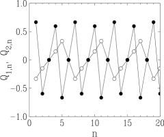
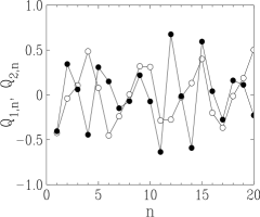
Figure 5: Plots of the current amplitudes $Q_{1,n}$ (full symbols) and $Q_{2,n}$ (empty symbols) against level number $n$, for $\Phi_{1}=BL_{1}^{2}/(4\pi)=\pi/3$. Left: commensurate case $L_{2}=2L_{1}$, i.e., $\omega=1/3$. Right: incommensurate case $\omega=1/\tau^{2}$.

Figure 6: Plots of the magnetization $M$ against $\Phi_{1}/(2\pi)=BL_{1}^{2}/(8\pi^{2})$, for $N=3$ (left) and $N=10$ (right). Full lines: $\omega=1/\tau^{2}$ (jumps due to twofold degeneracies are shown by symbols). Dashed lines: $\omega=1/{\rm e}$.

8 The rôle of spin-orbit interaction

So far spin did not play any role in our discussion. We now investigate the case that, besides the Abelian U(1) magnetic fluxes $\Phi_{1}$ and $\Phi_{2}$, there are also non-Abelian SU(2) fluxes $\Psi_{1}$ and $\Psi_{2}$.

For the sake of consistency, let us recall some basic notions pertaining to the physics of SU(2) fluxes. Such fluxes arise as a result of spin-orbit interaction. Unlike U(1) fluxes, SU(2) fluxes are invariant under time reversal. While the U(1) flux leading to the Aharonov-Bohm effect is realized by threading a ring with a magnetic field, the SU(2) flux leading to the Aharonov-Casher effect is generated by piercing a ring with a line of charge. More precisely, if a system of electrons is confined to a plane and subject to an electric field generated by a straight perpendicular charged wire with constant charge $\lambda$ per unit length, we have the SU(2) analogue of the Aharonov-Bohm effect. The starting point of the analysis is the Pauli Hamiltonian. In the presence of a vector potential ${\bm{A}}$ and of an electric field ${\bm{E}}$, within the approximate $\mathrm{U(1)}\otimes\mathrm{SU(2)}$ symmetry of the non-relativistic Schrödinger equation [12], this Hamiltonian reads, in dimensionful form,

$$H_{\mathrm{P}auli}=\frac{1}{2m}\left({\bm{p}}+\frac{e}{c}{{\bm{A}}}+\gamma\hbar{\bm{E}}\times{\bm{\sigma}}\right)^{2},$$ (8.1)

where $\gamma=e/(4mc^{2})$. The third term on the right-hand side of (8.1) is responsible for the spin-orbit interaction. In the case of a circular ring of radius $R$ pierced by a charged wire through its center, we have ${\bm{E}}=2\lambda{\bm{r}}/R^{2}$, whereas the curvilinear abscissa and the circumference read $s=R\theta$ and $L=2\pi R$. In this geometry, the U(1) and SU(2) potentials appearing in (8.1) can be eliminated locally by the respective gauge transformations

$$\matrix{\displaystyle g_{\mathrm{U}(1)}=\exp\left(-\frac{{\rm i}e}{\hbar c}\int_{0}^{s}{\bm{A}}\cdot{\rm d}{\bm{r}}\right)=\exp\left(-\frac{{\rm i}\Phi\theta}{2\pi}\right),\hfill\cr\displaystyle g_{\mathrm{S}U(2)}=\exp\left(-{\rm i}\gamma\int_{0}^{s}({\bm{E}}\times{\bm{\sigma}})\cdot{\rm d}{\bm{r}}\right)=\exp\left(-\frac{{\rm i}\Psi\,{\bm{{\hat{n}}}}\cdot{\bm{\sigma}}\,\theta}{2\pi}\right),}$$ (8.2)

where the integrations are carried out along the ring. In the above expression for $g_{\mathrm{S}U(2)}$, the integral need not be path-ordered. We have indeed $({\bm{E}}\times{\bm{\sigma}})\cdot{\rm d}{\bm{r}}=-({\bm{E}}\times{\rm d}{\bm{r}})\cdot{\bm{\sigma}}=-(2\lambda/R^{2})({\bm{r}}\times{\rm d}{\bm{r}})\cdot{\bm{\sigma}}=-2\lambda\,{\bm{{\hat{n}}}}\cdot{\bm{\sigma}}\,{\rm d}\theta$, where ${\bm{{\hat{n}}}}$ is the (properly oriented) unit vector perpendicular to the plane of the ring. As a result, the dimensionless SU(2) flux reads $\Psi=-4\pi\gamma\lambda$. The above simplifying property is specific of the case where the electric field lies in the plane in which the electrons are confined. It has also been used in a spherical geometry, in deriving a tight-binding version of the ${\bm{L}}\cdot{\bm{S}}$ spin-orbit interaction [13]. The SU(2) flux appears as a ‘pure gauge’, in the sense that it only affects the phase of the wavefunction. However, the U(1) and SU(2) potentials cannot be eliminated globally. These potentials rather give rise to non-integrable phase factors, ${\rm e}^{{\rm i}\Phi}$ for U(1) and ${\rm e}^{{\rm i}\Psi\,{\bm{{\hat{n}}}}\cdot{\bm{\sigma}}}$ for SU(2). Observables are therefore $2\pi$-periodic both in $\Phi$ and in $\Psi$. The upshot of the above discussion is that, in the ring geometry, the Pauli Hamiltonian can be replaced by a simpler one, namely

$$H=\left(p-a-b\,{\bm{{\hat{n}}}}\cdot{\bm{\sigma}}\right)^{2},$$ (8.3)

with the notations $p=-{\rm i}{\rm d}/{\rm d}s$, $a=\Phi/L$ and $b=\Psi/L$. For a single ring in the $(x,y)$ plane, we have ${\bm{{\hat{n}}}}={\bm{{\hat{z}}}}$, so that $s_{z}$ is conserved. The problem then reduces to that of two independent Aharonov-Bohm systems of polarized electrons, one with flux $\Phi+\Psi$ and the second with flux $\Phi-\Psi$.

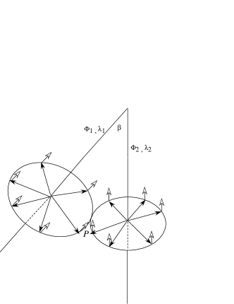
Figure 7: Gedankenexperimental realization of the two rings with U(1) and SU(2) fluxes such that spin is not conserved. Solid lines represent magnetic fluxes $\Phi_{1}$ and $\Phi_{2}$ as well as charged wires with respective longitudinal charge densities $\lambda_{1}$ and $\lambda_{2}$. Full arrows mark the direction of the electric fields, whereas empty arrows indicate the directions of the spins (more precisely, ${\hat{\bf n}}_{1,2}$). This is the special case corresponding to the Hamiltonian (8.4) where the two axes ${\hat{\bf n}}_{1,2}$ lie in the same $(x,z)$ plane.

A somewhat less simple manifestation of the AC effect in terms of SU(2) fluxes occurs when $s_{z}$ is not conserved. This can be realized (for example) by considering two rings in different planes respectively subject to perpendicular magnetic fields and pierced by perpendicular lines of charges with uniform densities $\lambda_{1}$ and $\lambda_{2}$. Such a Gedankenexperiment is schematically displayed in Figure 7. Thus, while in the U(1) two-ring problem the geometric configuration of the two rings (in particular their relative orientation) did not play an important rôle, the sample’s geometry becomes of central importance when SU(2) fluxes are considered. This situation allows one to study the influence of SU(2) fluxes on the U(1) magnetization [14]. The main messages of the analysis given below are as follows. (i) Even when ${\bm{{\hat{n}}}}_{1}$ is antiparallel to ${\bm{{\hat{n}}}}_{2}$, the non-conservation of $s_{z}$ requires both U(1) fluxes to be non-trivial, i.e., neither integer nor half-integer. This is a novel situation where the energy levels are sensitive to a combination of AB and AC effects. (ii) Even though $\Psi$ enters as a pure gauge, spin-orbit interaction might change the sign of the magnetization, so that the system switches between a paramagnetic and a diamagnetic response. (iii) In complete analogy with the U(1) case, where the orbital magnetization is related to the derivative of the ground-state energy with respect to $\Phi$, it is natural to define an ‘SU(2) magnetization’ related to the derivative of the ground-state energy with respect to $\Psi$. This magnetization is another equilibrium property. In each ring and for a given level $n$, it is proportional to the expectation value of the commutator $\{\hat{v},{\bm{{\hat{n}}}}\cdot{\bm{\sigma}}\}$, where ${\hat{v}}$ is the velocity operator. Thus, it can in principle be measured, despite the fact that the SU(2) (spin) current is not conserved while the U(1) (charge) current is.

The one-electron Hamiltonian of our two-ring system now reads

$${\cal H}=\left(p_{1}-a_{1}-b_{1}\,{\bm{{\hat{n}}}}_{1}\cdot{\bm{\sigma}}\right)^{2}+\left(p_{2}-a_{2}-b_{2}\,{\bm{{\hat{n}}}}_{2}\cdot{\bm{\sigma}}\right)^{2},$$ (8.4)

where $p_{1}$ and $p_{2}$ are the differential operators of (2.3), ${\bm{{\hat{n}}}}_{1}$ and ${\bm{{\hat{n}}}}_{2}$ are two arbitrary unit vectors, ${\bm{\sigma}}$ is the vector of Pauli matrices, whereas the U(1) vector potentials $a_{1}$ and $a_{2}$ and their SU(2) analogues $b_{1}$ and $b_{2}$ are related to the corresponding fluxes as follows:

$$a_{1}=\frac{\Phi_{1}}{L_{1}},\quad a_{2}=\frac{\Phi_{2}}{L_{2}},\quad b_{1}=\frac{\Psi_{1}}{L_{1}},\quad b_{2}=\frac{\Psi_{2}}{L_{2}},$$ (8.5)

The problem mostly depends on the angle $\beta$ between both directions ${\bm{{\hat{n}}}}_{1}$ and ${\bm{{\hat{n}}}}_{2}$ in spin space, such that ${\bm{{\hat{n}}}}_{1}\cdot{\bm{{\hat{n}}}}_{2}=\cos\beta$. For convenience we choose axes such that ${\bm{{\hat{n}}}}_{1}=(0,0,1)$ is along the $z$-axis whereas ${\bm{{\hat{n}}}}_{2}=(\sin\beta,0,\cos\beta)$ is in the $(x,z)$ plane.

A state $|\psi\rangle$ is described by a pair of wavefunctions $\{{\bm{\psi}}^{(1)}(s_{1}),\;{\bm{\psi}}^{(2)}(s_{2})\}$, each of them being a two-component spinor. Separating spin and orbital degrees of freedom, we are led to look for an eigenstate of ${\cal H}$ in the form

$${\bm{\psi}}^{(1)}(s_{1}) = \pmatrix{1\cr 0}{\rm e}^{{\rm i}(a_{1}+b_{1})s_{1}}(A_{1}\,{\rm e}^{{\rm i}qs_{1}}+B_{1}\,{\rm e}^{-{\rm i}qs_{1}})$$ (8.6)

$$+ \pmatrix{0\cr 1}{\rm e}^{{\rm i}(a_{1}-b_{1})s_{1}}(C_{1}\,{\rm e}^{{\rm i}qs_{1}}+D_{1}\,{\rm e}^{-{\rm i}qs_{1}}),$$ (8.7)

$${\bm{\psi}}^{(2)}(s_{2}) = \pmatrix{\cos\frac{\beta}{2}\cr\sin\frac{\beta}{2}}{\rm e}^{{\rm i}(a_{2}+b_{2})s_{2}}(A_{2}\,{\rm e}^{{\rm i}qs_{2}}+B_{2}\,{\rm e}^{-{\rm i}qs_{2}})$$ (8.8)

$$+ \pmatrix{-\sin\frac{\beta}{2}\cr\cos\frac{\beta}{2}}{\rm e}^{{\rm i}(a_{2}-b_{2})s_{2}}(C_{2}\,{\rm e}^{{\rm i}qs_{2}}+D_{2}\,{\rm e}^{-{\rm i}qs_{2}}).$$ (8.9)

Along the lines of Section 2, the continuity conditions generalizing (2.5) allow one to express the eight amplitudes $A_{1},\dots,D_{2}$ in terms of the two components of ${\bm{\psi}}({\mathrm{P}})$. The current conservation conditions generalizing (2.7) then yield the characteristic equation $D_{\rm SO}(q)=0$, with

$$D_{\rm SO}(q) = \Bigl{(}\sin q(L_{1}+L_{2})-\cos(\Phi_{2}+\Psi_{2})\sin qL_{1}-\cos(\Phi_{1}+\Psi_{1})\sin qL_{2}\Bigr{)}$$ (8.10)

$$\times \Bigl{(}\sin q(L_{1}+L_{2})-\cos(\Phi_{2}-\Psi_{2})\sin qL_{1}-\cos(\Phi_{1}-\Psi_{1})\sin qL_{2}\Bigr{)}$$

$$+ 4\,\sin qL_{1}\,\sin qL_{2}\,\sin\Phi_{1}\,\sin\Phi_{2}\,\sin\Psi_{1}\,\sin\Psi_{2}\,\sin^{2}\frac{\beta}{2}.$$

The first two lines of this expression are identical to the scalar characteristic equation (2.11), up to the replacement of the magnetic fluxes by the sums and differences of their Abelian and non-Abelian parts: $\Phi_{1}\to\Phi_{1}\pm\Psi_{1}$, $\Phi_{2}\to\Phi_{2}\pm\Psi_{2}$. Each factor therefore describes a scalar problem in an effective Abelian flux. The third line provides the coupling between both spin components. In order for this coupling to be non-zero, the four fluxes need to be simultaneously non-trivial, i.e., not equal to 0 or $\pi\ {\rm(mod.}\ 2\pi)$, and the angle $\beta$ not equal to $0\ {\rm(mod.}\ 2\pi)$.

In the case of two equal rings ($L_{1}=L_{2}=L$, $\Phi_{1}=\Phi_{2}=\Phi$, $\Psi_{1}=\Psi_{2}=\Psi$), the spectrum consists of an alternation of groups of two degenerate idle states, such that $\sin qL=0$, i.e., $qL=p\pi$, and of groups of two non-degenerate active states, such that

$$\cos qL=\cos\theta_{\pm}=\cos\Phi\cos\Psi\pm\sin\Phi\sin\Psi\cos\frac{\beta}{2},$$ (8.11)

Choosing for definiteness $0\leq\beta\leq\pi$, we have $0\leq\theta_{+}\leq\theta_{-}\leq\pi$. For $N=2$ electrons, only the first two active states are occupied. The magnetization reads

$$M=-\frac{1}{2\pi}\left(\theta_{+}\,\frac{\partial\theta_{+}}{\partial\Phi}+\theta_{-}\,\frac{\partial\theta_{-}}{\partial\Phi}\right).$$ (8.12)

Figure 8: Plots of the magnetization $M$ of two electrons on two equal rings, against $\Phi/\pi$, for $\Psi=\pi/2$ (left) and $\Psi=\pi/5$ (right). In both cases, $\beta=k\pi/10$, with $k=0,\dots,10$, bottom to top in the left part of the curves.

Let us consider the dependence of $M$ on the Abelian flux $\Phi$ in the range $0\leq\Phi\leq\pi$ and for $0\leq\Psi\leq\pi$. For $\beta=0$, we obtain

$$M=\left\{\matrix{-\Phi/\pi\hfill&\hbox{for}&0\leq\Phi<\pi-\Psi,\cr(\pi-\Phi)/\pi&\hbox{for}&\pi-\Psi<\Phi\leq\pi.\hfill}\right.$$ (8.13)

This discontinuous jump in the magnetization is rounded for non-zero values of $\beta$, as shown in Figure 8. This figure also illustrates a remarkable feature of such a simple system of two electrons on two equal rings, namely that the magnetization changes sign as a function of parameters. For a small magnetic flux $\Phi$, we have

$$M=-\frac{1}{\pi}\left(\cos^{2}\frac{\beta}{2}+\sin^{2}\frac{\beta}{2}\,\Psi\cot\Psi\right)\Phi+\cdots$$ (8.14)

The expression in the parentheses vanishes for

$$\tan^{2}\frac{\beta}{2}=-\frac{\tan\Psi}{\Psi},$$ (8.15)

provided $\Psi>\pi/2$. More generally, the magnetization vanishes along a $\Psi$-dependent curve in the $(\Phi,\beta)$ plane, shown in Figure 9. At fixed $\Psi$, the magnetization is positive above and to the right of that curve, whereas it is negative below and to the left of that curve.

Figure 9: Plot of the locus in the $(\Phi,\beta)$ plane where the magnetization $M$ of two electrons on two equal rings vanishes, at fixed $\Psi$. From top right to bottom left, $\Psi/\pi=0.1$, 0.2, 0.3, 0.4, 0.45, 0.49, 0.5 (vertical line), 0.51, 0.55, 0.6, 0.7, 0.8 and 0.9.

9 Discussion

The many differences between the single and the double-ring geometry, which have been underlined throughout this work, testify the importance of topology in mesoscopic physics. From a local viewpoint, both systems are governed by the same one-dimensional Schrödinger equation. They only differ in their global topological structure, measured by their genus (number of holes).

Another example underlining the key rôle of topology in the context of persistent currents has been studied by a collaboration involving one of us [15]. The importance of the sample’s topology in mesoscopic physics has already been stressed by Schmeltzer [10], who studied the persistent current of spinless fermions in a double-ring system, using the formalism of Dirac constraints. In fact, Schmeltzer’s work was the main motivation for the present research. Apart from underlining the importance of topology, the work [10] however focussed on different aspects. In particular, the rôle of spin and the AC effect were not tackled.

We have not tackled the rich physics that should emerge when interaction effects are taken into account. First of all, there are interesting charging effects, suggested and discussed for the single-ring geometry in [16, 17]. Second, interactions in one dimension turn the system to a non-Fermi liquid. While this problem has been studied for a single ring [18], persistent currents in interacting quantum rings have recently been studied in [19]. It can however be anticipated that the detailed analysis presented here for the non-interacting system will turn its place to a complicated and somewhat intractable formalism, so that e.g. the fine effects of length and flux commensurability will be absent.

The two-ring geometry provides a playground for testing fundamental aspects of quantum mechanics, such as the occurrence of interlaced AB and AC effects. At the same time, a two-ring system is certainly within the reach of fabrication (see Figure 1 in [20]), so that the present study is also rooted into the real world. At the same time, the difficulties of controlling the external electric field in semiconductor heterostructures hosting a two-dimensional electron gas, as well as their enhancement by internal fields of ion cores and discontinuities (eventually manifest as spin-orbit couplings) have recently been summarized in a comprehensive review article [21]. Thus, while the bare Hamiltonian (8.4) of course applies for any field whatsoever, a realization of the two-ring geometry as in Figure 7 is still to be considered as a Gedankenexperiment. Nevertheless, the main conclusion of our analysis is fundamental and should pass any experimental test, namely, an AC effect which is a pure gauge (periodic in the SU(2) phase) and does not conserve $s_{z}$ is realizable only if the AB effect is present.

Finally, although the present work has focussed onto zero-temperature equilibrium properties, it can be expected that transport properties will reveal a similar richness of behavior.

Appendix A One single ring: a reminder

In this Appendix we give a brief reminder of the well-known situation of a single clean ring. The ring with length $L$ and area $A$ is threaded by a flux $\Phi=BA$. It may assume an arbitrary planar shape. With the same conventions as in the body of this work, parametrizing a point of the wire by its curvilinear abscissa $s$ in the range $0\leq s\leq L$, the one-body Hamiltonian reads

$${\cal H}=(p-a)^{2},$$ (1.1)

with $p=-{\rm i}\,{\rm d}/{\rm d}s$ and $a=\Phi/L$.

It is worth mentioning the analogy with Bloch theory, already noticed in [2]. Starting from the Schrödinger equation ${\cal H}\psi=E\psi$ with $\psi(s+L)=\psi(s)$, a gauge transformation $\psi(s)={\rm e}^{{\rm i}as}\eta(s)$ leads to the following equation and boundary condition for $\eta(s)$:

$$p^{2}\eta(s)=E\eta(s),\quad\eta(s+L)={\rm e}^{{\rm i}\Phi}\eta(s).$$ (1.2)

This is exactly the equation for an electron in a one-dimensional lattice potential of period $L$ and Bloch wavenumber $K$ such that $KL=\Phi$, i.e., $K=a=\Phi/L$. One immediate consequence is that the energy is periodic in $\Phi$ with period $2\pi$. This results also holds when the ring is not clean, since the full (disordered) potential can still be viewed as a periodic potential of period $L$.

The eigenstates of ${\cal H}$ are given by the wavefunctions

$$\psi(s)\sim{\rm e}^{{\rm i}(q+a)s}.$$ (1.3)

The periodicity of $\psi(s)$ in $s$ with period $L$ yields the quantization condition $(q+a)L=2\pi k$, hence

$$q_{k}=\frac{2\pi k-\Phi}{L},$$ (1.4)

where $k=0,\pm 1,\dots$ The wavefunctions $\psi_{k}(s)\sim\exp(2\pi{\rm i}ks)$ therefore do not depend on the magnetic flux $\Phi$.

The contributions $I_{k}$ and $M_{k}$ of the eigenstate number $k$ to the persistent current and the magnetization read

$$I_{k}=-\frac{\partial E_{k}}{\partial\Phi}=\frac{2q_{k}}{L},\quad M_{k}=-\frac{\partial E_{k}}{\partial B}=AI_{k}.$$ (1.5)

With the notation (3.4), the above result for $I_{k}$ simply reads $Q_{k}=1$.

For a zero-temperature system with $N$ electrons, and for $0\leq\Phi\leq\pi$, we have the following results.

• For $N=2p-1$ odd, the occupied states are $k=-p+1,\dots,p-1$. We obtain

  $$E=E_{0}+\frac{N}{L^{2}}\,\Phi^{2},\quad M=-\frac{2A}{L^{2}}\,N\Phi.$$ (1.6)

• For $N=2p$ even, the occupied states are $k=-p+1,\dots,p$. We obtain

  $$E=E_{0}+\frac{N}{L^{2}}\,(\pi-\Phi)^{2},\quad M=\frac{2A}{L^{2}}\,N(\pi-\Phi).$$ (1.7)

In both cases the minimum energy reads $E_{0}=N(N^{2}-1)\pi^{2}/(3L)$. For a circular ring with radius $R$, we have $L=2\pi R$ and $A=\pi R^{2}$, so that $2A/L^{2}=1/(2\pi)$.

Appendix B Three coupled rings

In this Appendix we show how the present investigation can be extended to more complex geometries. We consider for definiteness the case of a sample made of three unequal rings touching at two contact points P and Q, as shown in Figure 10. The line PQ is assumed to be an axis of symmetry of the sample. The left, middle and right rings have respective lengths $L_{1}$, $L_{2}$ and $L_{3}$ and areas $A_{1}$, $A_{2}$ and $A_{3}$. They are therefore threaded by magnetic fluxes $\Phi_{1}=BA_{1}$, $\Phi_{2}=BA_{2}$ and $\Phi_{3}=BA_{3}$.

Figure 10: The sample considered in Appendix B is made of three unequal rings touching at two contact points P and Q.

The one-electron Hamiltonian of the system reads

$${\cal H}=(p_{1}-a_{1})^{2}+(p_{2}-a_{2})^{2}+(p_{3}-a_{3})^{2},$$ (2.1)

with $p_{1}=-{\rm i}\,{\rm d}/{\rm d}s_{1}$, $p_{2}=-{\rm i}\,{\rm d}/{\rm d}s_{2}$, $p_{3}=-{\rm i}\,{\rm d}/{\rm d}s_{3}$, $a_{1}=\Phi_{1}/L_{1}$, $a_{2}=\Phi_{2}/L_{2}$, $a_{3}=\Phi_{3}/L_{3}$.

A state is now described by three wavefunctions, one living on each ring: $\{\psi^{(1)}(s_{1}),\;\psi^{(2)}(s_{2}),\;\psi^{(3)}(s_{3})\}$. These wavefunctions obey two continuity conditions of the form (2.5) (one at P and one at Q) and two current conservation conditions of the form (2.7). Along the lines of Section 2, we obtain the characteristic function

$$D_{3}(q) = \cos q(L_{1}+L_{2}+L_{3})$$ (2.2)

$$- \cos\Phi_{3}\cos q(L_{1}+L_{2})-\cos\Phi_{1}\cos q(L_{2}+L_{3})$$ (2.3)

$$+ \cos\Phi_{3}\cos qL_{1}+\cos\Phi_{1}\cos\Phi_{3}\cos qL_{2}+\cos\Phi_{1}\cos qL_{3}$$ (2.4)

$$+ \cos\Phi_{2}\sin qL_{1}\sin qL_{3}-\cos qL_{1}\cos qL_{3}-\cos\Phi_{1}\cos\Phi_{3}.$$ (2.5)

Many of the outcomes of this paper can be extended to the present situation, although expressions become very cumbersome. The energy eigenvalues $E_{n}=q_{n}^{2}$ can be parametrized as

$$q_{n}=\frac{n\pi+g_{n}}{L_{1}+L_{2}+L_{3}}\quad(n=1,2,\dots),$$ (2.6)

where the modulation $g_{n}$ obeys the bounds $-\pi\leq g_{n}\leq 2\pi$. In the absence of magnetic fluxes, the factorized form (4.1) of the characteristic function generalizes to

$$D_{3}(q)=8\,\sin\frac{q(L_{1}+L_{2}+L_{3})}{2}\,\sin\frac{qL_{1}}{2}\,\sin\frac{qL_{2}}{2}\,\sin\frac{qL_{3}}{2}.$$ (2.7)

The spectrum consists of four sectors. The corresponding states can be respectively referred to as trilateral, left, central and right.

References

References

- [1] Imry Y 1997 Introduction to Mesoscopic Physics (Oxford: Oxford University Press) Akkermans E and Montambaux G 2007 Mesoscopic Physics of Electrons and Photons (Cambridge: Cambridge University Press)
- [2] Büttiker M, Imry Y, and Landauer R 1983 Phys. Lett. A 96 365 Cheung H F, Gefen Y, Riedel E K, and Shih W H 1988 Phys. Rev. B 37 6050
- [3] Lévy L P, Dolan G, Dunsmuir J, and Bouchiat H 1990 Phys. Rev. Lett. 64 2074 Chandrasekhar V, Webb R A, Brady M J, Ketchen M B, Gallagher W J, and Kleinsasser A 1991 Phys. Rev. Lett. 67 3578
- [4] Neder I, Heiblum M, Levinson Y, Mahalu D, and Umansky V 2006 Phys. Rev. Lett. 96 016804 Neder I, Ofek N, Chung Y, Heiblum M, Mahalu D, and Umansky V 2007 Nature 448 333
- [5] Aharonov Y and Bohm D 1959 Phys. Rev. 115 485
- [6] Webb R A, Washburn S, Umbach C P, and Laibowitz R B 1985 Phys. Rev. Lett. 54 2696
- [7] Byers N and Yang C N 1961 Phys. Rev. Lett. 7 46 Bloch F 1970 Phys. Rev. B 2 109
- [8] Aharonov Y and Casher A 1984 Phys. Rev. Lett. 53 319
- [9] Mathur H and Stone A D 1992 Phys. Rev. Lett. 68 2964
- [10] Schmeltzer D 2008 J. Phys.: Condens. Matter 20 335205
- [11] Aubry S 1978 Solitons and Condensed Matter Physics Solid State Science Series ed A R Bishop and T Schneider Springer Series in Solid State Science 8 264 Aubry S 1980 Ferroelectrics 24 53 Aubry S and André G 1980 Ann. Israel Phys. Soc. 3 133 Bak P 1982 Rep. Prog. Phys. 45 587
- [12] Fröhlich J and Studer U M 1993 Rev. Mod. Phys. 65 733
- [13] Avishai Y and Luck J M 2008 J. Stat. Mech. P06008
- [14] Meir Y, Gefen Y, and Entin-Wohlman O 1989 Phys. Rev. Lett. 63 798
- [15] Yakubo K, Avishai Y, and Cohen D 2003 Phys. Rev. B 67 125319
- [16] Cedraschi P and Büttiker M 1998 J. Phys. Cond. Matt. 10 3985
- [17] Büttiker M and Stafford C A 1996 Phys. Rev. Lett. 76 495
- [18] Loss D and Martin T 1993 Phys. Rev. B 47 4619
- [19] Castelano L K, Hai G Q, Partoens B, and Peeters F M 2008 Phys. Rev. B 78 195315
- [20] Kuznetsov V I, Firsov A A, Dubonos S V, and Chukalina M V 2007 Bulletin of the Russian Academy of Sciences: Physics 71 1083 [arXiv:cond-mat/0712.1602]
- [21] Fabian J, Matos-Abiague A, Ertler C, Stano P, and Zutic I 2007 Acta Physica Slovaca 57 565