T-matrix calculation via Dicrete-dipole approximation and exploiting mirror symmetry

Abstract

We present three methods for calculating the T-matrix for modeling arbitrarily shaped micro-sized objects. When applied to microrotors, their rotation and mirror symmetry can be exploited to reduce memory usage and calculation time by 2 orders of magnitude. In the methods where the T-matrix elements are calculated using point matching with vector spherical fields, mode redundancy can be exploited to reduce calculation time.

I Introduction

• Motivation: optical rotors

• DDA Purcell1973; Draine1994

• Memory requiements of the A matrix, swapping

• Compressed A matrix

• T-matrix Waterman1971

• DDA T-matrix Mackowski2002

Our T-matrix methods are

• near VSWF field point matching with DDA field

• far VSWF field point matching with DDA field

• rotate Choi1999 and translate Videen2000

II Optimizing the Discrete Dipole Approximation interaction matrix

The size of the microdevices we model may exceed 10–20 wavelengths in size, which may well require computational time in excess of several days and RAM beyond that available. To circumvent these limitations, we exploit the discrete rotational and/or mirror symmetry of a microcomponent. This is closely tied with the link between DDA and the T-matrix method. In the T-matrix method, the fields are represented as sums of vector spherical wavefunctions (VSWFs) Waterman1971; Nieminen2003b, and to use DDA to calculate a T-matrix, we can simply calculate the scattered field (and its VSWF representation) for each possible incident single-mode VSWF field in turn. The important point is that each VSWF is characterized by a simple azimuthal dependence of $\exp(\mathrm{i}m\phi)$, where $m$ is the azimuthal mode index.

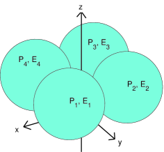
Figure 1:

If we consider a group of dipoles that are rotationally symmetric about the vertical axis—in the case of figure 1, there is 4th-order rotational symmetry—the magnitude of the incident field will be the same, the field differing by the vector rotation 6 and phase factor of $\exp(\mathrm{i}m\phi)$; only the dipole moment of one repeating unit of the total number of dipoles needs to be known. In spherical coordinates,

$$\vec{P}_{q}^{sph}=\vec{P}_{1}^{sph}exp(\mathrm{i}m\phi_{q}).$$ (1)

However, our implementation of the interaction matrixDraine1994, electric field and dipole moments were in cartesian coordinates system(what was the advantage?). This requires a transformation of the dipole moment at the first segment from the cartesian to spherical coordinate system followed by a transformation back from spherical to cartesian at the rotational counterpart dipole,

$$\vec{P}_{q}^{cart}=C_{q}S\vec{P}_{1}^{cart}exp(\mathrm{i}m\phi_{q}),$$ (2)

where

$$S=\left[\begin{array}[]{ccc}sin(\theta)cos(\phi_{1})&sin(\theta)sin(\phi_{1})&cos(\theta)\\ cos(\theta)cos(\phi_{1})&cos(\theta)sin(\phi_{1})&-sin(\theta)\\ -sin(\phi_{1})&cos(\phi_{1})&0\end{array}\right]$$ (3)

is an orthogonal matrix that transforms the $\vec{P}_{1}^{cart}$ vector into the spherical coordinate system and

$$C_{q}=\left[\begin{array}[]{ccc}sin(\theta)cos(\phi_{q})&sin(\theta)sin(\phi_{q})&cos(\theta)\\ cos(\theta)cos(\phi_{q})&cos(\theta)sin(\phi_{q})&-sin(\theta)\\ -sin(\phi_{q})&cos(\phi_{q})&0\end{array}\right]^{-1}$$ (4)

is a transpose of $S$ but at the azimuthal coordinate of the rotational counterpart dipole.

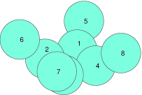
(a) (b)

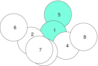
Figure 2: (a) 8-dipole example. (b) The 2 dipoles required to completely specify all dipole moments.

This brings up question of how to reduce the number of equations such that only one rotational unit needs to be solved. Conventionally, the interaction matrix as defined in Draine1994 represents the coupling between each dipole with all other dipoles. Figure 3(a) shows the interaction matrix for the example set of dipoles shown in figure 2(a). In general the matrix will be made up of $N\times N$ cells for $N$ dipoles; each cell is a $3\times 3$ tensor. In the example, the matrix is made up of $8\times 8$ cells. A diagonal cell represents the self interaction (or the inverse of the polarizability) and an off-diagonal cell represents the coupling between different dipoles. Taking advantage of the equal amplitudes and known phase factors between a dipole and its rotational counterparts, we can reduce the interaction matrix. Taking the example in figure 2(b), we contruct the interaction matrix as if there were only 2 dipoles but we aggregate the contribution from the appropriate dipoles. For the off-diagonal cells, the coupling between a dipole with the other dipoles including their rotational counterparts are summed as follows

$$\bar{A}_{jk} = \sum^{Q}_{q=1}\frac{\exp(\mathrm{i}kr_{jk}^{(q)})}{r_{jk}^{(q)}}$$ (5)

$$\times\left[k^{2}(\hat{r}_{jk}^{(q)}\hat{r}_{jk}^{(q)}-I_{3})+\frac{\mathrm{i}kr_{jk}^{(q)}-1}{r_{jk}^{2(q)}}(3\hat{r}_{jk}^{(q)}\hat{r}_{jk}^{(q)}-I_{3})\right]$$

$$\times\;C_{q}S\exp(\mathrm{i}m\phi),\;j\neq k,$$

where $Q$ is the order of discrete rotational symmetry, $m$ is the azimuthal mode of the incident VSWF field, $q$ is the rotational segment number, the rotational angle $\phi=2\pi q/Q$, $r_{jk}^{(q)}$ is the distance from points $r_{j}$ to the rotationally symmetric points $r_{k}^{(q)}$, and $\hat{r}_{jk}^{(q)}$ is the unit vector from points $r_{j}$ to $r_{k}^{(q)}$. The coordinate for a given rotational symmetric point is calculated using a rotation about the z-axis,

$$r_{k}^{(q)}=\left[\begin{array}[]{ccc}cos(q\phi)&-sin(q\phi)&0\\ sin(q\phi)&cos(q\phi)&0\\ 0&0&1\end{array}\right]r_{k}.$$ (6)

For the diagonal cells, the “self interaction” includes the coupling between a dipole and its rotational counterparts:

$$\bar{A}_{jj} = \alpha^{-1}_{j}+\sum^{Q}_{q=2}\frac{\exp(\mathrm{i}kr_{jk}^{(q)})}{r_{jk}^{(q)}}$$ (7)

$$\times\left[k^{2}(\hat{r}_{jk}^{(q)}\hat{r}_{jk}^{(q)}-I_{3})+\frac{\mathrm{i}kr_{jk}^{(q)}-1}{r_{jk}^{2(q)}}(3\hat{r}_{jk}^{(q)}\hat{r}_{jk}^{(q)}-I_{3})\right]$$

$$\times\;C_{q}S\exp(\mathrm{i}m\phi),\;j=k.$$

Figure 3(b) shows the interaction matrix representation for the example dipole system in figure 2(c). The compressed interaction matrix is a factor of $Q^{2}$ smaller than the conventional matrix.

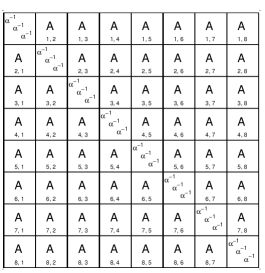
(a) (b)

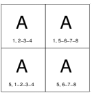
Figure 3: (a) Full interaction matrix. (b) Symmetry reduced interaction matrix

Having precalculated the incident fields $\vec{E}_{j,inc}$ at each dipole of the rotational unit, we solve for the dipole moments $\vec{P}_{j}$ for the dipoles with a reduced set of linear equations. The dipole moments and fields of the rotational counterpart dipoles can be calculated by applying the rotational matrix 6 and phase factor $exp(\mathrm{i}m\phi)$.

We can exploit mirror symmetry in a similar fashion, since the VSWFs possess either even or odd parity w.r.t. the $xy$-plane. This allows a reduction in size by a further factor of 4.

III Methods for calculating the T-matrix

III.1 Near field point matching

• vswf field matched with DDA field

• solve for p’s and q’s

• contract T-matrix column by column

$$p_{nm}=\vec{M}_{nm}^{(1)}(kr)/\vec{E}_{DDA,TEnm},$$ (8)

$$q_{nm}=\vec{N}_{nm}^{(1)}(kr)/\vec{E}_{DDA,TMnm}$$ (9)

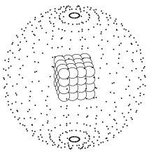
(a) (b)

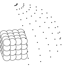
Figure 4: (a) Near field matching. (b) Octant near field matching.

III.2 Far field matching

• DDA farfield

• VSH farfield

• solving for $p_{nm}$ and $q_{nm}$

• Constructing the T-matrix

Far field matching

$$\vec{M}_{nm}^{(1,2)}(kr)=\frac{N_{n}}{kr}(\mp\mathrm{i})^{n+1}exp(\pm\mathrm{i}kr)\vec{C}_{nm}(\theta,\phi)$$ (10)

$$\vec{N}_{nm}^{(1,2)}(kr)=\frac{N_{n}}{kr}(\mp\mathrm{i})^{n+1}exp(\pm\mathrm{i}kr)\vec{B}_{nm}(\theta,\phi)$$ (11)

$$kr\vec{E}(\theta,\phi)=\sum_{nm}a_{nm}B_{nm}+b_{nm}C_{nm}+c_{nm}P_{nm}$$ (12)

$$p_{nm}N_{n}(-\mathrm{i})^{n+1}=b_{nm},$$ (13)

$$q_{nm}N_{n}(\mathrm{i})^{n}=a_{nm}$$ (14)

$$p_{nm}=\frac{b_{nm}}{N_{n}(-\mathrm{i})^{n+1}},$$ (15)

$$q_{nm}=\frac{a_{nm}}{N_{n}(\mathrm{i})^{n}}$$ (16)

III.3 Rotation and translation of vector fields

• Videen translations Videen2000, precalculated

• Rotations of axes

• Constructing the T-matrix, cycle through m’s and n’s

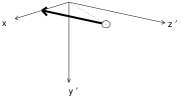
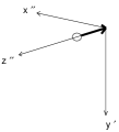
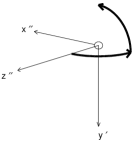
a) b)
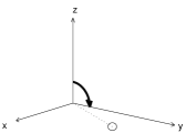
c) d)
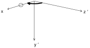
e) f) g)

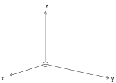
Figure 5: a) $z=0$ translation b) $z$ onto $y$ axis rotation c) $z^{\prime}=0$ translation d) $z^{\prime}$ onto $x$ axis rotation e) $z^{\prime\prime}=0$ translation f) rotations back onto the original $z$-axis g) original orientation

IV Mode redundancy and the order of discrete rotational symmetry

• Motivation, computational savings

• Explain mth order discrete rotational symmetry and VSWF m modes

• redundant modes

• Floquet’s theorem

• mscat = minc +ip (5)

• For a cube, p = 4, and mscat = minc,minc 4,minc 8, ….

• time saving

V Results

V.1 Phase functions for the spheres and cubes

comparision

• Sphere Mie soln

• cube point matching Nieminen2007a (toolbox)

• also Wriedt Wriedt1998a

a)
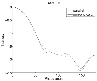
b)

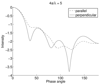
Figure 6: The phase function for cubes with the refractive index of $1.5$ and widths of a) $0.75\lambda$ b) $1.25\lambda$.

V.2 Cross rotor torque calculations

• convergence of torque

• low nrel so $\lambda/5$ suffices

• reference Theo’s results

VI Conclusion

Combination of optimization techniques

• DDA rotational and mirror symm, interaction matrix compression

• Far field and near field matrix, octant matching grid points

• exploiting mode redundancy