Solution of Maxwell’s equations on a de Sitter background

Abstract

The Maxwell equations for the electromagnetic potential, supplemented by the Lorenz gauge condition, are decoupled and solved exactly in de Sitter space-time studied in static spherical coordinates. There is no source besides the background. One component of the vector field is expressed, in its radial part, through the solution of a fourth-order ordinary differential equation obeying given initial conditions. The other components of the vector field are then found by acting with lower-order differential operators on the solution of the fourth-order equation (while the transverse part is decoupled and solved exactly from the beginning). The whole four-vector potential is eventually expressed through hypergeometric functions and spherical harmonics. Its radial part is plotted for given choices of initial conditions. We have thus completely succeeded in solving the homogeneous vector wave equation for Maxwell theory in the Lorenz gauge when a de Sitter spacetime is considered, which is relevant both for inflationary cosmology and gravitational wave theory. The decoupling technique and analytic formulae and plots are completely original. This is an important step towards solving exactly the tensor wave equation in de Sitter space-time, which has important applications to the theory of gravitational waves about curved backgrounds.

1 Introduction

It is by now well known that the problem of solving vector and tensor wave equations in curved spacetime, motivated by physical problems such as those occurring in gravitational wave theory and relativistic astrophysics, is in general a challenge even for the modern computational resources. Within this framework, a striking problem is the coupled nature of the set of hyperbolic equations one arrives at. For example, on using the Maxwell action functional

$$S=-{1\over 4}\int_{M}F_{ab}F^{ab}\sqrt{-g}\;d^{4}x$$ (1)

jointly with the Lorenz PHMAA-34-287 gauge condition

$$\nabla^{b}A_{b}=0,$$ (2)

one gets, in vacuum, the coupled equations for the electromagnetic potential

$$\left(-\delta_{a}^{\;b}\leavevmode\thinspace\hbox{\vrule\vtop{\vbox{\hrule\kern 1.0pt\hbox{\vphantom{\tt/}\thinspace{\tt\ }\thinspace}} \kern 1.0pt\hrule}\vrule}\thinspace+R_{a}^{\;b}\right)A_{b}=0.$$ (3)

It was necessary to wait until the mid-seventies to obtain a major breakthrough in the solution of coupled hyperbolic equations such as (3), thanks to the work of Cohen and Kegeles PHRVA-D10-1070 , who reduced the problem to the task of finding solutions of a complex scalar equation. Even on considering specific backgrounds such as de Sitter spacetime, only the Green functions of the wave operator have been obtained explicitly so far CMPHA-103-669 , to the best of our knowledge.

Thus, in a recent paper 00436 , we have studied the vector and tensor wave equations in de Sitter space-time with static spherical coordinates, so that the line element reads as

$$ds^{2}=-f\;dt^{2}+f^{-1}\;dr^{2}+r^{2}(d\theta^{2}+\sin^{2}\theta d\phi^{2}),$$ (4)

where $f\equiv 1-H^{2}r^{2}$, and $H$ is the Hubble constant related to the cosmological constant $\Lambda$ by $H^{2}={\Lambda\over 3}$. The vector field $X$ solving the vector wave equation can be expanded in spherical harmonics according to PHRVA

$$X = {\widetilde{Y}}_{lm}(\theta)e^{-i(\omega t-m\phi)}\Bigr{[}f_{0}(r)dt+f_{1}(r)dr\Bigr{]}$$ (5)

$$+ e^{-i(\omega t-m\phi)}\left[-{mr\over\sin\theta}f_{2}(r){\widetilde{Y}}_{lm}(\theta)+f_{3}(r){d{\widetilde{Y}}_{lm}\over d\theta}\right]d\theta$$

$$+ ie^{-i(\omega t-m\phi)}\left[-r\sin\theta f_{2}(r){d{\widetilde{Y}}_{lm}\over d\theta}+mf_{3}(r){\widetilde{Y}}_{lm}(\theta)\right]d\phi,$$

where ${\widetilde{Y}}_{lm}(\theta)$ is the $\theta$-dependent part of the spherical harmonics $Y_{lm}(\theta,\phi)$. As we have shown in 00436 , the function $f_{2}$ is decoupled and obeys a differential equation solved by a combination of hypergeometric functions, i.e.

$$f_{2}(r)=f^{-i\Omega/2}\biggr{[}U_{1}r^{l}F\left(a_{-},a_{+};{3\over 2}+l;H^{2}r^{2}\right)+U_{2}r^{-l-1}F\left(a_{+},a_{-};{1\over 2}-l;H^{2}r^{2}\right)\biggr{]},$$ (6)

where

$$\Omega\equiv{\omega\over H},\;a_{\pm}\equiv-{1\over 4}\left({2i\Omega}-3-2l\pm 1\right).$$ (7)

At this stage, however, the problem remained of solving explicitly also for $f_{0}(r),f_{1}(r),f_{3}(r)$ in the expansion (5). For this purpose, Sec. II derives the decoupling procedure for such modes in de Sitter, and Sec. III writes explicitly the decoupled equations. Section IV solves explicitly for $f_{0},f_{1},f_{3}$ in terms of hypergeometric functions, while Sec. V plots such solutions for suitable initial conditions. Relevant details are presented in the Appendices. It now remains to be seen whether a technique similar to Secs. II and III can be used to solve completely also the tensor wave equation obtained in 00436 . This technical step would have far reaching consequences for the theory of gravitational waves in cosmological backgrounds, as is stressed in 00436 , and we hope to be able to perform it in a separate paper.

2 Coupled modes

Unlike $f_{2}$, the functions $f_{0},f_{1}$ and $f_{3}$ obey instead a coupled set, given by Eqs. (54), (55), (57) of 00436 , which are here written, more conveniently, in matrix form as (our $L\equiv l(l+1)$, and we set $\epsilon=1$ in the Eqs. of 00436 , which corresponds to studying the vector wave equation (3))

$$\left(\begin{array}[]{ccc}P_{00}&A_{3}&0\\ f^{-2}A_{3}&P_{11}&r^{-2}f^{-1}LC_{3}\\ 0&C_{3}&P_{33}\end{array}\right)\,\left(\begin{array}[]{l}f_{0}\\ f_{1}\\ f_{3}\end{array}\right)=0,$$ (8)

having defined

$$A_{3}\equiv{2i\Omega H^{3}r\over f},$$ (9)

$$C_{3}\equiv{2\over r},$$ (10)

$$P_{00}\equiv{d^{2}\over dr^{2}}+Q_{1}{d\over dr}+Q_{2},$$ (11)

$$P_{11}\equiv{d^{2}\over dr^{2}}+Q_{3}{d\over dr}+Q_{4},$$ (12)

$$P_{33}\equiv{d^{2}\over dr^{2}}+Q_{5}{d\over dr}+Q_{6},$$ (13)

$$Q_{1}\equiv C_{3}={2\over r},$$ (14)

$$Q_{2}\equiv{\Omega^{2}H^{2}\over f^{2}}-{L\over r^{2}f},$$ (15)

$$Q_{3}\equiv{6\over r}\left(1-{2\over 3}{1\over f}\right),$$ (16)

$$Q_{4}\equiv{\Omega^{2}H^{2}\over f^{2}}-\left(4H^{2}+{(L+2)\over r^{2}}\right){1\over f},$$ (17)

$$Q_{5}\equiv{2\over r}\left(1-{1\over f}\right),$$ (18)

$$Q_{6}\equiv{\Omega^{2}H^{2}\over f^{2}}-{L\over r^{2}}{1\over f},$$ (19)

where we have corrected misprints on the right-hand side of Eqs. (54) and (55) of 00436 . With our notation, the three equations resulting from (8) can be written as

$$P_{00}f_{0} = -A_{3}f_{1},$$ (20)

$$P_{11}f_{1} = -{A_{3}\over f^{2}}f_{0}-{LC_{3}\over r^{2}f}f_{3},$$ (21)

$$P_{33}f_{3} = -C_{3}f_{1}.$$ (22)

3 Decoupled equations

We now express $f_{1}$ from Eq. (20) and we insert it into Eq. (21), i.e.

$$P_{11}\left(-{1\over A_{3}}P_{00}f_{0}\right)=-{A_{3}\over f^{2}}f_{0}-{LC_{3}\over r^{2}f}f_{3}.$$ (23)

Next, we exploit the Lorenz gauge condition (2), i.e. 00436

$$Lf_{3}=r^{2}f{d\over dr}\left(-{1\over A_{3}}P_{00}f_{0}\right)-2r(1-2f)\left(-{1\over A_{3}}P_{00}f_{0}\right)+i{\Omega Hr^{2}\over f}f_{0},$$ (24)

and from Eqs. (23) and (24) we obtain, on defining the new independent variable $x=rH$, the following fourth-order equation for $f_{0}$:

$$\left[{d^{4}\over dx^{4}}+B_{3}(x){d^{3}\over dx^{3}}+B_{2}(x){d^{2}\over dx^{2}}+B_{1}(x){d\over dx}+B_{0}(x)\right]f_{0}(x)=0,$$ (25)

where

$$B_{0}(x)\equiv{b_{0}(x)\over x^{4}(x^{2}-1)^{4}},$$ (26)

$$b_{0}(x)\equiv L(L-2)+2L(2-L-\Omega^{2})x^{2}+\Bigr{[}\Omega^{4}+4\Omega^{2}+L(L+2(\Omega^{2}-1))\Bigr{]}x^{4},$$ (27)

$$B_{1}(x)\equiv{4(\Omega^{2}+L-2+6x^{2})\over x(x^{2}-1)^{2}},$$ (28)

$$B_{2}(x)\equiv{2\Bigr{[}-L+(\Omega^{2}+L-14)x^{2}+18x^{4}\Bigr{]}\over x^{2}(x^{2}-1)^{2}},$$ (29)

$$B_{3}(x)\equiv{4(-1+3x^{2})\over x(x^{2}-1)}.$$ (30)

Eventually, $f_{1}$ and $F_{3}\equiv Hf_{3}$ can be obtained from Eqs. (20) and (24), i.e.

$$f_{1}(x)={i\over 2\Omega}{(1-x^{2})\over x}\left({d^{2}\over dx^{2}}+{2\over x}{d\over dx}+{\Omega^{2}\over(1-x^{2})^{2}}-{L\over x^{2}(1-x^{2})}\right)f_{0}(x),$$ (31)

$$LF_{3}(x)=\left[x^{2}(1-x^{2}){d\over dx}-2x(2x^{2}-1)\right]f_{1}(x)+i\Omega{x^{2}\over(1-x^{2})}f_{0}(x).$$ (32)

Our $f_{1}$ and $f_{3}$ are purely imaginary, which means we are eventually going to take their imaginary part only. Moreover, as a consistency check, Eqs. (31) and (32) have been found to agree with Eq. (22), i.e. (22) is then identically satisfied.

4 Exact solutions

Equation (25) has four linearly independent integrals, so that its general solution involves four coefficients of linear combination $C_{1},C_{2},C_{3},C_{4}$, according to (hereafter, $F$ is the hypergeometric function already used in (6))

$$f_{0}(x) = C_{1}x^{-1-l}(1-x^{2})^{-{i\over 2}\Omega}F\left(-{i\over 2}\Omega-{l\over 2},-{i\over 2}\Omega+{1\over 2}-{l\over 2};{1\over 2}-l;x^{2}\right)$$ (33)

$$+ C_{2}x^{-1-l}(1-x^{2})^{-{i\over 2}\Omega}F\left(-{i\over 2}\Omega+1-{l\over 2},-{i\over 2}\Omega-{1\over 2}-{l\over 2};{1\over 2}-l;x^{2}\right)$$

$$+ C_{3}x^{l}(1-x^{2})^{-{i\over 2}\Omega}F\left(-{i\over 2}\Omega+{l\over 2},-{i\over 2}\Omega+{3\over 2}+{l\over 2};{3\over 2}+l;x^{2}\right)$$

$$+ C_{4}x^{l}(1-x^{2})^{-{i\over 2}\Omega}F\left(-{i\over 2}\Omega+1+{l\over 2},-{i\over 2}\Omega+{1\over 2}+{l\over 2};{3\over 2}+l;x^{2}\right).$$

Regularity at the origin ($x=0$ should be included, and we recall that the event horizon for an observer situated at $x=0$ is given by $x=1$ BOUCHER ) implies that $C_{1}=C_{2}=0$, and hence, on defining

$$a_{1}\equiv-{i\over 2}\Omega+{l\over 2},\;b_{1}\equiv-{i\over 2}\Omega+{3\over 2}+{l\over 2},\;d_{1}\equiv{3\over 2}+l,$$ (34)

we now re-express the regular solution in the form (the points $x=0,1$ being regular singular points of the equation (25) satisfied by $f_{0}$)

$$f_{0}(x)=x^{l}(1-x^{2})^{-{i\over 2}\Omega}\Bigr{[}C_{3}F(a_{1},b_{1};d_{1};x^{2})+C_{4}F(a_{1}+1,b_{1}-1;d_{1};x^{2})\Bigr{]},$$ (35)

where the second term on the right-hand side of (35) can be obtained from the first through the replacements

$$C_{3}\rightarrow C_{4},\;a_{1}\rightarrow a_{1}+1,\;b_{1}\rightarrow b_{1}-1,$$

and the series expressing the two hypergeometric functions are conditionally convergent, because they satisfy ${\it Re}(c-a-b)=i\Omega$, with

$$a=a_{1},a_{1}+1;\;b=b_{1},b_{1}-1;\;c=d_{1}.$$

Last, we exploit the identity

$${d\over dz}F(a,b;c;z)={ab\over c}F(a+1,b+1;c+1;z)$$ (36)

to find, in the formula (31) for $f_{1}(x)$,

$${d\over dx}f_{0}(x)=C_{3}\biggr{\{}x^{l-1}(1-x^{2})^{-{i\over 2}\Omega-1}\Bigr{[}l(1-x^{2})+i\Omega x^{2}\Bigr{]}F(a_{1},b_{1};d_{1};x^{2})$$ (37)

$$+ {2a_{1}b_{1}\over d_{1}}x^{l+1}(1-x^{2})^{-{i\over 2}\Omega}F(a_{1}+1,b_{1}+1;d_{1}+1;x^{2})\biggr{\}}$$

$$+ \Bigr{\{}C_{3}\rightarrow C_{4},\;a_{1}\rightarrow a_{1}+1,\;b_{1}\rightarrow b_{1}-1\Bigr{\}}.$$

It is then straightforward, although tedious, to obtain the second derivative of $f_{0}$ (see Eq. (38) of Appendix A) in the equation for $f_{1}$, and the third derivative of $f_{0}$ in the formula (32) for $Hf_{3}$. The results are exploited to plot the solutions in Sec. V.

In general, for given initial conditions at $\alpha\in[0,1[$, one can evaluate $C_{3}$ and $C_{4}$ from

$$f_{0}(\alpha)=\beta,\;f_{0}^{\prime}(\alpha)=\gamma,$$

i.e. $C_{3}=C_{3}(\beta,\gamma),C_{4}=C_{4}(\beta,\gamma)$.

5 Plot of the solutions

To plot the solutions, we begin with $f_{0}$ as given by (35), which is real-valued despite the many $i$ factors occurring therein. Figures 1 to 3 describe the solutions for the two choices $C_{3}=0,C_{4}=1$ or the other way around, and various values of $l$ and $\Omega$.

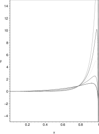
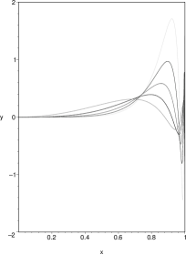
Figure 1: Regular solution (35) for $f_{0}$ with $C_{3}=0,C_{4}=1,l=2,\ldots 6$ with $\Omega=2$ (left figure) and $\Omega=4$ (right figure). Increasing values of $l$ correspond to more peaked curves on the right part of the plots.

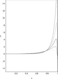
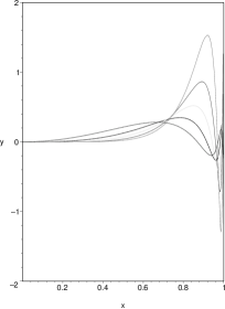
Figure 2: Regular solution (35) for $f_{0}$ with $C_{3}=1,C_{4}=0,l=2,\ldots 6$ with $\Omega=2$ (left figure) and $\Omega=4$ (right figure). Increasing values of $l$ correspond to more peaked curves on the right part of the plots.

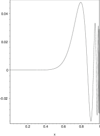
Figure 3: Regular solution (35) for $f_{0}$ with $C_{3}=0,C_{4}=1,l=10$ and $\Omega=10$.

We next plot $f_{1}/i$ and $F_{3}/i\equiv Hf_{3}/i$ by relying upon (31) and (32). As far as we can see, all solutions blow up at the event horizon, corresponding to $x=1$, since there are no static solutions of the wave equation which are regular inside and on the event horizon other than the constant one BOUCHER .

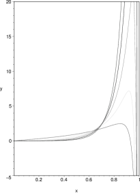
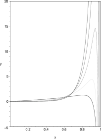
Figure 4: Regular solution (31) for $f_{1}/i$ with $C_{3}=1,C_{4}=0$ (left figure) and $C_{3}=0,C_{4}=1$ (right figure) for $l=2\ldots 6$ and $\Omega=2$.

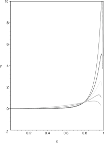
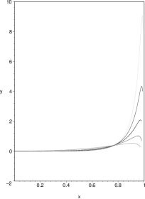
Figure 5: Regular solution (32) for $F_{3}/i$ with $C_{3}=0,C_{4}=1$ (left figure) and $C_{3}=1,C_{4}=0$ (right figure) for $l=2\ldots 6$ and $\Omega=2$.

Appendix A Derivatives of $f_{0}$

The higher-order derivatives of $f_{0}$ in sections III and IV get increasingly cumbersome, but for completeness we write hereafter the result for $f_{0}^{\prime\prime}(x)$, i.e.

$${d^{2}\over dx^{2}}f_{0}(x) = C_{3}\biggr{\{}{4a_{1}(a_{1}+1)b_{1}(b_{1}+1)\over d_{1}(d_{1}+1)}x^{l+1}(1-x^{2})^{-{i\over 2}\Omega}F(a_{1}+2,b_{1}+2;d_{1}+2;x^{2})$$ (38)

$$+ x^{l-1}(1-x^{2})^{-{i\over 2}\Omega-1}{2a_{1}b_{1}\over d_{1}}x$$

$$\times [(2l+1)(1-x^{2})+2i\Omega x^{2}]F(a_{1}+1,b_{1}+1;d_{1}+1;x^{2})$$

$$+ x^{l-2}(1-x^{2})^{-{i\over 2}\Omega-2}\biggr{[}l(l-1)(x^{2}-1)^{2}-{i\Omega\over 2}(x^{2}-1)(lx+2(l+1)x^{2})$$

$$+ (2i\Omega-\Omega^{2})x^{4}\biggr{]}F(a_{1},b_{1};d_{1};x^{2})\biggr{\}}$$

$$+ \biggr{\{}C_{3}\rightarrow C_{4},\;a_{1}\rightarrow a_{1}+1,\;b_{1}\rightarrow b_{1}-1\biggr{\}}.$$

Appendix B Special cases: $l=0$ and $l=1$

We list here the main equations for $l=0,1$ for completeness. These equations do not add too much to the above discussion and hence we have decided to include them in the appendix.

B.1 The case $l=0,m=0$

In this case we have $Y(\theta)=(4\pi)^{-1/2}=$ constant and the only surviving functions are $f_{0}$ and $f_{1}$. The main equations in 00436 reduce then to (recalling that our Eq. (3) requires setting $\epsilon=1$ in 00436 )

$$\frac{d^{2}f_{0}}{dx^{2}}=-\frac{2}{x}\frac{df_{0}}{dx}-\frac{\Omega^{2}}{(x^{2}-1)^{2}}f_{0}+\frac{2i\Omega x}{(x^{2}-1)}f_{1}$$ (39)

and the Lorenz gauge condition (24) which now becomes

$$\Omega f_{0}=i(x^{2}-1)^{2}\frac{df_{1}}{dx}+\frac{2i(x^{2}-1)(2x^{2}-1)}{x}f_{1}\,.$$ (40)

These equations can be easily separated and explicitly solved in terms of hypergeometric functions. The details are not very illuminating and are therefore omitted.

B.2 The case $l=1,m=0,1$

In this case we have

$$Y = \sqrt{\frac{3}{4\pi}}\cos\theta\,\quad l=1,m=0$$

$$Y = -\sqrt{\frac{3}{8\pi}}\sin\theta\,\quad l=1,m=1\ .$$ (41)

However, by virtue of the spherical symmetry of the background, the equations for both cases $l=1,m=0$ and $l=1,m=1$ do coincide. We have

$$\frac{d^{2}f_{0}}{dx^{2}} = -\frac{2}{x}\frac{df_{0}}{dx}-\frac{(\Omega^{2}x^{2}+2x^{2}-2)}{x^{2}(x^{2}-1)^{2}}f_{0}+\frac{2i\Omega x}{(x^{2}-1)}f_{1},$$

$$\frac{d^{2}f_{1}}{dx^{2}} = -\frac{2(3x^{2}-1)}{x(x^{2}-1)}\frac{df_{1}}{dx}-\frac{(\Omega^{2}x^{2}+4x^{4}-4)}{x^{2}(x^{2}-1)^{2}}f_{1}+\frac{2i\Omega x}{(x^{2}-1)^{3}}f_{0}$$

$$+\frac{4F_{3}}{x^{3}(x^{2}-1)},$$

$$\frac{d^{2}f_{2}}{dx^{2}} = -\frac{2(2x^{2}-1)}{x(x^{2}-1)}\frac{df_{2}}{dx}-\frac{(\Omega^{2}x^{2}+2x^{4}-2)}{x^{2}(x^{2}-1)^{2}}f_{2},$$

$$\frac{d^{2}F_{3}}{dx^{2}} = -\frac{2x}{(x^{2}-1)}\frac{dF_{3}}{dx}-\frac{(\Omega^{2}x^{2}+2x^{2}-2)}{x^{2}(x^{2}-1)^{2}}F_{3}-\frac{2}{x}f_{1}.$$ (42)

To this set one has to add the Lorenz gauge condition (24), which now reads

$$\Omega f_{0}=i(x^{2}-1)^{2}\frac{df_{1}}{dx}+\frac{2i(x^{2}-1)}{x^{2}}[F_{3}+f_{1}x(2x^{2}-1)]\,.$$ (43)

Once more, the detailed discussion of this case can be performed by repeating exactly the same steps as in the general case, and is hence omitted.

References

- (1) Lorenz, L.: Phil. Mag. 34, 287 (1867).
- (2) Cohen, J.M., Kegeles, L.S.: Phys. Rev. D 10, 1070 (1974).
- (3) Allen, B., Jacobson, T.: Commun. Math. Phys. 103, 669 (1986).
- (4) Bini, D., Capozziello, S., Esposito, G.: Int. J. Geom. Meth. Mod. Phys. 5, 1069 (2008).
- (5) Zerilli, F.J.: Phys. Rev. D 9, 860 (1974).
- (6) Boucher, W., Gibbons, G.W.: in The Very Early Universe, eds. S.W. Hawking, G.W. Gibbons, S.T.C. Siklos, Cambridge University Press, Cambridge, 1983.