Abelian Higgs Cosmic Strings: Small Scale Structure and Loops
Abstract
Classical lattice simulations of the Abelian Higgs model are used to investigate small scale structure and loop distributions in cosmic string networks. Use of the field theory ensures that the small-scale physics is captured correctly. The results confirm analytic predictions of Polchinski & Rocha Polchinski and Rocha (2006) for the two-point correlation function of the string tangent vector, with a power law from length scales of order the string core width up to horizon scale with evidence to suggest that the small scale structure builds up from small scales. An analysis of the size distribution of string loops gives a very low number density, of order 1 per horizon volume, in contrast with Nambu-Goto simulations. Further, our loop distribution function does not support the detailed analytic predictions for loop production derived by Dubath et al. Dubath et al. (2008). Better agreement to our data is found with a model based on loop fragmentation Scherrer and Press (1989), coupled with a constant rate of energy loss into massive radiation. Our results show a strong energy loss mechanism which allows the string network to scale without gravitational radiation, but which is not due to the production of string width loops. From evidence of small scale structure we argue a partial explanation for the scale separation problem of how energy in the very low frequency modes of the string network is transformed into the very high frequency modes of gauge and Higgs radiation. We propose a picture of string network evolution which reconciles the apparent differences between Nambu-Goto and field theory simulations.
I Introduction
Cosmic strings are line-like objects formed in the early universe (for reviews see Hindmarsh and Kibble (1995); Vilenkin and Shellard (1994); Sakellariadou (2007)). They exist as solitons in theories with spontaneously broken symmetries if the vacuum manifold is not simply connected Kibble (1976), or as fundamental objects in string theory Copeland et al. (2004). A network of cosmic strings may form in thermal phase transitions Kibble (1976), at the end of hybrid inflation Yokoyama (1989); Kofman et al. (1994); Copeland et al. (1994), or at the end of brane inflation when brane and anti-brane annihilate Sarangi and Tye (2002); Dvali and Vilenkin (2004). They remain of immense cosmological interest through their appearance in these high energy physics models, and further motivation is provided from the enhanced fit of the CDM model to Cosmic Microwave Background (CMB) data when cosmic strings are included Battye et al. (2006); Bevis et al. (2008) (see also Bevis et al. (2004); Wyman et al. (2005); Fraisse (2007); Battye et al. (2008); Urrestilla et al. (2008)). Calculations of the CMB signal at small angular scales Fraisse et al. (2007); Pogosian et al. (2008) and in the polarisation B-mode Bevis et al. (2007a); Pogosian and Wyman (2008) show that future CMB observations will further constrain cosmological models with strings.
Cosmic strings form networks of infinitely long string and loops, where a string can be called “infinite” in cosmological terms if it is larger than the horizon. Infinite string takes the form of a random walk with correlation length . The network evolves in a self-similar manner, keeping at about the horizon scale, an important dynamical feature known as scaling. Scaling means that the energy density of infinite strings decreases as , ( is cosmic time), and thus constitutes a constant fraction of the total.
Since the original string network scaling paradigm was introduced Kibble (1976, 1980); Vilenkin (1981) a broad picture of the cosmological evolution of string networks has emerged, using a mixture of calculation, numerical simulation, and analytic modelling. Yet, a major unsolved problem is the eventual destination of the energy in the infinite strings. This is of notable importance and greatly limits our ability to constrain string scenarios via their decay products, such as gravitational waves or energetic particles.
In the traditional picture, string will loop back on itself and undergo a self-intersection event, which then results in the loop being cut from the long string. Strings have tension, so loops tend to collapse inwards and can shrink to a point. In their final moments, as their radius becomes close to the string width, they give up their energy in a burst of particle emission, which in principle might be detectable via cosmic rays. However whilst they are shrinking, they would oscillate and emit gravitational waves. Conventionally it is taken that the loops are large relative to the string width and that these gravitational waves take away most of the energy.
Numerical simulations using the Nambu-Goto approximation Albrecht and Turok (1989); Bennett and Bouchet (1990); Allen and Shellard (1990), in which the strings are modelled as relativistic one-dimensional entities, seemed to support this picture. Copious loop production was observed at scales a small fraction of the cosmological horizon, along with the presence of small-scale structure in the correlation functions of the long string. The small-scale structure is related to the creation of small-scale loops, but progress on understanding the connection has been slow.
It is crucial to establish the dominant length scale of loop production, as it controls both the amplitude and frequency of the gravitational wave signal, and the fraction of energy going into ultra-high energy cosmic rays. The current debate is summarised in Section V. Here we merely note that there is a great deal of uncertainty over the loop population of cosmic string networks and the Minkowski-space Nambu-Goto simulations have been used to argue that loop production might even peak on the scale of the string width Vincent et al. (1997a).
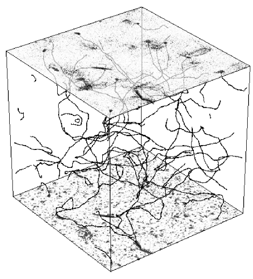
If this is true, it is necessary to go beyond the Nambu-Goto approximation and calculate with the underlying theory. The Nambu-Goto approximation also breaks down at kinks (discontinuities in the string tangent vector) and cusps (points where the tangent vector vanishes and the string doubles back), which are universal and common features of a string network. The underlying theory for solitonic strings is a quantum field theory: Fortunately, quantum corrections appear to be small Borsanyi and Hindmarsh (2008), and classical field theory should be a good approximation. Numerical simulations in the classical Abelian Higgs model Vincent et al. (1998); Moore et al. (2002) showed that infinite string does indeed scale by losing energy into gauge and Higgs radiation (see Fig. 1), although it was not established whether the decay proceeded via short-lived loops at the size of the string core width, or directly from the long strings themselves. In any case, no sign of copious loop production was found. In this paper we present evidence that direct radiation is much more important than small loop production for Abelian Higgs string networks.
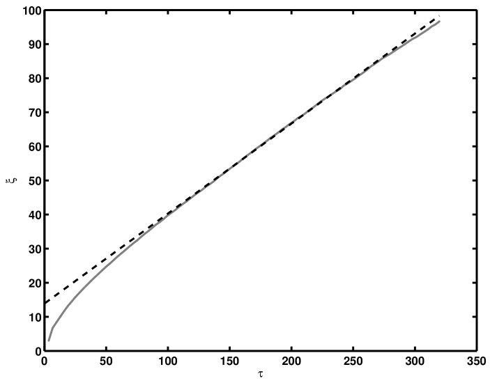
The idea of direct radiation raises a puzzle: in order to create radiation in a mode with mass , the field must be oscillating at a frequency . A smooth string curved on the horizon scale is constructed from field modes with frequencies . In view of the mismatch it was argued that gauge and Higgs radiation must be negligible Everett (1981). Numerical simulations of smooth strings Olum and Blanco-Pillado (2000) show that radiation is indeed suppressed by a factor exponential in the ratio of the curvature radius to the string width. Nevertheless, simulations exhibit scaling behaviour at times when the network length scale exceeds the string width by a factor Vincent et al. (1998); Moore et al. (2002); Bevis et al. (2007b), and for example in Fig. 2 we see that this is confirmed to in our larger simulations.
It should be noted that a similar puzzle was presented by the small size (compared with the horizon scale) of loops in Nambu-Goto simulations. Recent work by Polchinski and collaborators Polchinski and Rocha (2006, 2007); Dubath et al. (2008) has resolved the problem by showing how small-scale structure can give rise both to apparently smooth strings and to loop production at the small-scale cut-off on the string network.
Motivated by the success of the approach by Polchinksi and collaborators Polchinski and Rocha (2006); Dubath et al. (2008), we analyse the small scale structure of cosmic strings in the Abelian Higgs model through the two-point tangent vector correlator and the loop distribution function. We find excellent agreement for the two-point tangent vector correlator, showing that its slope at short distances and the mean square velocity are related as predicted by their model but with mean square velocities found to be significantly lower in Abelian Higgs simulations than in Nambu-Goto simulations. The presence of small-scale structure on Abelian Higgs strings leads us to propose that the high frequencies required for direct radiation are generated in much the same way as small loops.
However, the prediction for the form of the loop production function is much less successful, even after taking into account the fact that in field theory simulations loops lose energy and shrink at a constant rate. From evidence found of fragmentation of horizon size loops we are prompted to compare our data to the model of Scherrer & Press Scherrer and Press (1989) and this seems to provide a better explanation.
We also investigate the speed with which the network relaxes to scaling, and in particular how quickly the small scale structure appears. We find evidence that the relaxation time goes roughly as the initial network length scale. Furthermore, we present evidence that small scale structure grows from the bottom up, rather than resulting from a cascade from large scales as has hitherto been assumed Polchinski and Rocha (2006).
Our paper is laid out as follows. A review of the traditional picture of energy loss from cosmic strings is provided in Sec. II then the particulars of the field theory simulation for Abelian Higgs strings are outlined in Sec. III. Results of the analysis of the two-point correlation functions and loop distributions are discussed in Sec. IV and Sec. V. We summarise our results in Sec. VI and present a picture of string network evolution which reconciles our results with those derived from Nambu-Goto simulations.
II Energy Loss Mechanisms
Conventional “solitonic” cosmic strings are produced in a symmetry-breaking phase transition at a scale , in a field theory with coupling constant , and typical mass scale . They have linear mass density and have width . For example, strings produced at the Grand Unification energy scale have GeV, and gravitational coupling .
A particularly important feature in string energy loss is the presence of cusps, points where the speed of the string becomes the speed of light. This produces a singularity in the shape of the string where the tangent vector to the loop vanishes. The string is bent back on itself and has the opportunity to interact with itself over the length of the cusp region. Also important are kinks, formed during intercommutation when there are sharp changes in the tangent vector. These discontinuities then resolve themselves into kinked waves travelling in both directions away from the intercommutation site. Numerical simulations based on the Nambu-Goto equations show a large number of intercommutations, forcing a build up of small scale structure. When oppositely-moving modes interact they can emit gravitational radiation, and the resulting back reaction Hindmarsh (1990) can smooth the kinks, as shown in numerical simulations Quashnock and Spergel (1990).
Conventionally, three main energy loss mechanisms have been considered, all of which take place on loops which have broken off from the long string network. Perturbative production of particles from the coupling to the Higgs field for strings with can be calculated to produce a flux of high energy particles with power Srednicki and Theisen (1987)
| (1) |
where is the size of the loop. Where string is overlapping in cusp regions, it can annihilate releasing energy in the form of high energy particles. The original estimate Brandenberger (1987) was corrected in Blanco-Pillado and Olum (1999) who obtained
| (2) |
The power emitted through gravitational radiation, , from a sizeable oscillating string loop of length and mass can be estimated from its quadrupole moment Weinberg (1972); Vachaspati and Vilenkin (1985).
| (3) |
Much additional work has been done on the production of gravitational wave bursts at the sites of cusps on strings with and without additional small scale structure Damour and Vilenkin (2000, 2001); Siemens and Olum (2001, 2003a). Cusps on strings with small-scale structure are also sources of intense loop production Siemens and Olum (2003b); Dubath et al. (2008).
Purely based on the length dependence of these relations for the power output; gravitational radiation is the dominant decay channel for loops of length , where is the string core width. Below this length, cusp annihilation is is dominant. So it is of considerable importance to discover the distribution of different sized loops produced and evolving in the network as their size determines decay modes and the radiative by- products. This has crucial bearing on estimates of gravitational radiation or flux from high energy cosmic rays that we may be able to detect from a network of cosmic strings.
In the conventional cosmic string scenario the loop distribution is measured in simulations using the Nambu-Goto approximation and neglecting gravitational back-reaction. This is justifiable when the radius of curvature of the string is much greater than the string core width so a string can be assumed infinitely thin, and when the weak field approximation holds, . It is clear that in the presence of kinks and cusps, the Nambu-Goto approximation is strictly not justified, but it is assumed that gravitational radiation back-reaction will act to smooth the strings on a scale Polchinski and Rocha (2007), where is a small parameter defined below, and that large-scale properties will be reproduced correctly.
In the absence of back-reaction, Nambu-Goto simulations show that loops are produced at a small constant physical scale, which is most likely the initial correlation length of the network Ringeval et al. (2007); Martins and Shellard (2006); Olum and Vanchurin (2007). In Ref. Martins and Shellard (2006) there is a claim that there are signs that this scale is growing, while Ref. Olum and Vanchurin (2007) emphasises the significance of an apparently stable population of loops with sizes , arguing that the peak at the initial correlation length will eventually disappear.
In view of the automatic breakdown of the Nambu-Goto approximation when strings intercommute and produce kinks, it would seem sensible to simulate strings in an underlying field theory. One resolves the kinks and cusps correctly, and includes classical radiation as a form of energy loss. While the conventional arguments given above emphasise gravitational radiation, omitted from all simulations, one should be able to see the other forms of energy loss and to check their scaling with loop size. However, as outlined in the introduction, previous field theory simulations Vincent et al. (1998); Moore et al. (2002) found a scaling infinite string network without a significant population of loops. There appears to be an energy-loss mechanism allowing the strings to scale, which has a different length dependence to any of those outlined above.
To see this, consider a string network whose spatial distribution scales with the horizon size such that the length of string in an horizon volume is . The energy density of the string network hence varies as , which then requires the network to lose energy at a rate . Hence the rate of energy loss from a piece of string of size is . Thus a scaling network requires an energy loss mechanism which is independent of the size of the string, like gravitational radiation, but a factor stronger. One implication of the mechanism is that the length of a loop of string will shrink at a constant rate of order unity.
We verify this by running radiation era simulations for a very long time until there is only a single shrinking loop or a pair of straight strings winding around one or more directions in the simulation volume, which has periodic boundary conditions. The change in total comoving string length with conformal time is shown in Fig. 3 to be linear. By inspection one can see that for strings that are shrinking, as claimed. Once two strings in the box become straight their length oscillates around the box crossing distance, which is the behaviour expected in the Nambu-Goto approximation.

The detailed mechanism for this strong energy loss is not well understood. Attention has been focused on the production of ‘core’ sized loops Vincent et al. (1998); Moore et al. (2002), which would nicely connect the Nambu-Goto and field theory simulations. Core loops produced at the size of the string core width would quickly evaporate into classical radiation, and despite a large production rate would have a very low number density, which is easily estimated to be a few per Hubble volume Moore et al. (2002). In this scenario, field theory strings are behaving like Nambu-Goto strings in that loops are being produced at the smallest physical scale, which is in one case the string width, and the other the initial correlation length. While we see core loops, we would expect them to be associated with long string, and as we will show, we are unable to find such a correlation. Their number density is also too low to account for the energy loss from long string. It may be that energy is being broken off in lumps which are too small to register as loops at all.
III String simulation method
III.1 Abelian Higgs model
As discussed in the introduction, we characterise the small-scale structure and loop distribution of strings via simulation of the Abelian Higgs model Hindmarsh and Kibble (1995); Vilenkin and Shellard (1994); Sakellariadou (2007). This is the simplest field theory to contain local (or gauge) cosmic strings and has Lagrangian density:
| (4) |
where is a complex scalar Higgs field, is the gauge- covariant derivative and is the usual field strength tensor. String solutions are well known in this model Nielsen and Olesen (1973); the phase of the Higgs field winds around () as a closed loop is traversed through space and is forced to depart from the vacuum manifold over a tube of radius . The gauge field acts to compensate the winding but this results in a pseudo-magnetic flux tube of radius .
III.2 String width control
These two fixed physical length scales must be resolved in any simulation of the string network but, in an expanding Friedman-Robertson-Walker universe, they rapidly fall away from the other length scales that must also be resolved. Using comoving coordinates the horizon size is given simply by the conformal time and is the relevant length scale at which the super-horizon tangle of string begins to straighten and decay. However, the comoving string width decays as the reciprocal of the cosmic scale factor and therefore as in a radiation-dominated universe and under matter- domination. We therefore require to resolve two scales which diverge as under matter domination, which would, in principle, limit us to very short periods of simulation111That our simulations resolve the string width limits them in size to being far smaller than the horizon size at matter-radiation equality and therefore our simulations are also limited to much earlier times. However, we can simulate a matter dominated universe at very early times and use scaling to make statements about a matter dominated era at later times..
However in Ref. Bevis et al. (2007b), a technique was demonstrated via which the coupling constants and were raised to time dependent variables:
| (5) | |||||
| (6) |
in order that the comoving string width behaves as:
| (7) |
That is, gives the true dynamics while yields a comoving string width, which is particularly convenient for simulation. The dynamical equations derived upon variation of the action were then:
| (8) | |||
| (9) |
(in the gauge ) with the variation yielding the quasi-Gauss’ Law constraint:
| (10) |
Although these field equations do not conserve energy if (because the action is not time- translation invariant), the dynamics were shown in Ref. Bevis et al. (2007b) to be insensitive to . Indeed the difference in their results for the two-point correlation functions of the energy-momentum tensor between and in the radiation era, where was achievable, were found to be slight while their results for the CMB power spectra, which are dominated by the matter era, were found to be similarly insensitive to over the range to , with the later being the largest value at which reliable CMB results could be obtained.
Here we use the equations of motion Eqs. (8) and (9) with throughout, although we also check our results using simulations with for the radiation era (only), and find changes that are negligible. Note, however, that our equations of motion at are not precisely the same as those used in Ref. Moore et al. (2002).
III.3 Simulation Specifics
Eqs. (8) and (9) are discretised onto a lattice using the procedure described in Ref. Bevis et al. (2007b) and hereafter called LAH, which is an extension from Minkowski space-time to flat FRW universes of the standard approach of Ref. Moriarty et al. (1988). This preserves the Gauss’ law constraint to machine precision. Initial conditions were chosen following Ref. Bevis et al. (2007b) in order for a string network to emerge rapidly and the Gauss constraint obeyed. To achieve the latter, we set to zero the gauge field and the time derivatives of both the gauge and Higgs fields. To achieve the former, we set the simulation start time such that the horizon is comparable to the (uniform) lattice spacing and therefore the phase of scalar field is an independent random variable on each lattice site, while we set . We employ periodic boundary conditions and therefore the fields can be evolved forward reliably until the half-box crossing time for light.
We use a lattice spacing of and set , and , which together guarantee that strings are resolved for all when and for in our radiation era check. Note that the above scalings leave the ratio constant and we therefore study the model at the Bogomol’nyi value Bogomol’nyi (1976), which yields equal scalar and gauge masses. The simulations were performed using the UK National Cosmology supercomputer Cos , with parallel processing enabled via the LATfield library Bevis and Hindmarsh , using a lattice size of and averaging over 20 realisations. Additional simulations using a lattice were performed on the University of Sussex HPC Archimedes cluster.
We have been able to access a dynamic range of similar order to Nambu-Goto simulations performed by other groups working on small scale structure issues but due to the differences between the simulations the measures for dynamic range that are suitable in one case are ambiguous in another, making this a difficult comparison. On lattice volumes with , a network of strings of width is fully formed from conformal time and is simulated until , when the periodic boundary conditions of the simulation volume can potentially be felt. Checks of the full energy-momentum tensor indicate that scaling is achieved at around .
One measure of dynamic range is , which contains measurable quantities in our simulation. This can be compared with the ratio of the initial and final correlation lengths, ( Ringeval et al. (2007); Olum and Vanchurin (2007)) in Nambu-Goto simulations although the initial correlation length has no straightforward meaning in our simulation. Another measure is the ratio of the final time to the time at which the network achieves scaling. For us, gives us a dynamic range of about 2 (in conformal time) for our simulations and about 3 for lattices. Nambu-Goto simulations Ringeval et al. (2007) estimate a dynamical range of 5 from the scaling of the energy density of long string in the radiation era.
III.4 String length measurements
At intervals during the evolution we record the coordinates of lattice plaquettes around which the phase of has a net winding number222While a winding of the phase is gauge-invariant in the continuum, on a lattice it can be removed by a finite gauge transform. Therefore we employ the gauge- invariant measure of Ref. Kajantie et al. (1998). As a first approximation we then take it that a segment of string having length threads through each plaquette of winding and joins the centres of the lattice cells on either side. From these segments we can then construct the path of the string, although since it is composed of an array of perpendicular lengths the string length is overestimated. We do not attempt to smooth the paths in order to compensate, as in Refs. Vincent et al. (1998); Moore et al. (2002); Bevis and Saffin (2008), but instead apply a Scherrer-Vilenkin correction of Scherrer and Vilenkin (1998) to such length measurements. This factor is derived from the length of the line for a two-component Gaussian random field and so will not be completely accurate for our dynamic string network. However, the results for the average string length density are in approximate agreement with that measured using the Lagrangian density Fig. 4. This second method makes use of the fact that perturbative radiation makes zero contribution to , while a static straight string contributes at per unit length density. Since is a four-scalar and length density picks up a -factor upon a Lorentz transform, then is a measure of the (invariant) string length.
Rather than use the (comoving) string length density directly, we instead compare with the network length scale , defined as:
| (11) |
where is the reference volume and the string length within it. For a scaling network .
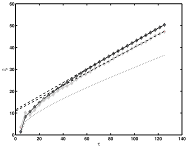
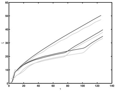
In Fig. 4, we plot both the Lagrangian measure result and the winding measure result (with no subscript since it is our default measure), which reveal a linear behaviour after an initial transient, consistent with the expected scaling. As pointed out in Ref. Bevis et al. (2007b), there is nothing fundamental about the value of and it is simply an artefact of the initial conditions. Indeed, this can be seen in Fig. 5, which shows additional results from two runs in which an artificial damping phase (similar to that used in Ref. Vincent et al. (1997b)) was employed for an extended time. As can be seen in the figure, when the damping is released, both these runs show rapidly reverting to approximately the same gradient as the undamped run. Reference Bevis et al. (2007b) also observed scaling with in the two-point correlation functions of the energy-momentum tensor, so there is no evidence from the simulations that this scaling is a transient. These energy-momentum correlators show that the network demonstrates scaling in a simulation over the conformal time range , which will be referred to as the scaling epoch.
IV Correlation Functions
IV.1 Tangent Vector Correlators
A 2-point correlation function from LAH simulation data is compared to analytic results which are reviewed in a manifest form with a view to introducing the variables and functions under discussion. For a thorough analysis refer to Polchinski and Rocha (2006); Dubath et al. (2008); Polchinski and Rocha (2007). The equations of motion are reformulated in terms of the left and right moving unit vectors p and q defined in terms of the position vector where is the string coordinate.
| (12) |
where dots are derivatives with respect to , primes with respect to and
| (13) |
thus giving the equations of motion in the transverse gauge Albrecht and Turok (1989)
| (14) | |||||
| (15) |
From the coordinate locations of the string extracted from LAH it is simple to compare the Euclidean distance between 2 points on the string and the separation along the string coordinate.
The longest string at a set of equally spaced times throughout the scaling epoch in the simulation is isolated for analysis in both the radiation and matter dominated eras. The comoving distance along the string along a string coordinate length is compared to the Euclidean distance, , between and . Along each loop of string, the mean square Euclidean distance is averaged over many starting points a few string segments apart around the loop, thus creating a 2-point function,
| (16) |
For consistency with notation used elsewhere Polchinski and Rocha (2006); Martins and Shellard (2006) and using in terms of the definitions of Eq. (12) we denote
Correlations for opposite moving modes will be subdominant to the build up of those moving in the same direction along the string . Identifying that , averaging over an ensemble of segments and many hubble times allows an approximation to first order of for small giving
The equations of motion can be rewritten in terms of the evolution of .
| (18) |
which integrates to the form
| (19) |
with defined as scale factor . The correlator must be a function of if it is to exhibit scaling. Given that , we need the time dependence of of (Eq. 13)
Hence
Given that Eq. (19) has a power law form
we find
| (20) |
The tangent vector correlator should also scale
| (21) | |||||
| (22) |
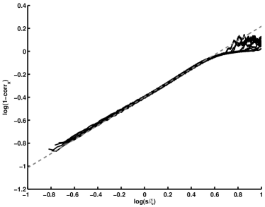
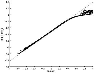
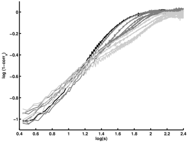
In order to test the prediction, the second derivative of the 2-point function is taken numerically to find a fit for the parameters in this analytic result. A least squares fit is used to optimise the parameters in the function for taking a nominal standard deviation equivalent to the length to weight smaller appropriately on the logarithmic scale. Noise is reduced by averaging the result over 20 simulations and additionally averaging over a block of and centring the mean value. It should be noted that the smoothing process was not found to alter the parameters or the shape of the function, notably at small , but allowed the least squares fit to converge more quickly. These functions are shown for the radiation era Fig. 6 and matter era Fig. 7 simulations. The correlations over long distances reflect smoothness on large scales and a clear power law demonstrated on smaller scales from a few times the correlation length down to string width scales. The average parameter values over 7 seven equally spaced times in the scaling epoch of the simulation have also been calculated for and as an investigation of transitions between eras. Results are given in Table 1.
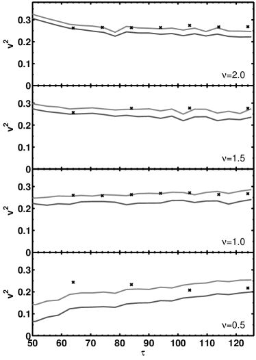
The parameter provides an estimate for the average network velocity squared via Eq. (20) and its value can be cross-checked with that calculated directly from the simulation Fig. 8. Two methods are used for estimating the average network velocity. One uses the electric and magnetic components from the field strength tensor and the other the canonical momentum and spatial gradients of the field, and . Denoting the estimators and , we have
| (23) |
and
| (24) |
where and are calculated using and respectively, and the subscript denotes a Lagrangian weighting of a field according to
We see that the measured velocities agree well with those inferred from the slope of the correlation function, strong evidence that the model of Polchinski and Rocha (2006) describes the dynamics of long string in the Abelian Higgs model well.
Finally we note that our root mean square (RMS) velocities are approximately in both the matter and radiation era. These are significantly lower than measured in Nambu-Goto simulations, about 0.66 in the radiation era and 0.61 in the matter era. This is likely to be a result of backreaction from massive radiation, not included in Nambu-Goto simulations. Our velocities are, however, in agreement with the uncorrected RMS velocities of Ref. Moore et al. (2002), which are measured in a field theory simulation using the positions of the zeros of the field.
IV.2 Initial Conditions and Relaxation to Scaling
It is important to test for any dependence of our results upon the initial conditions chosen and to fully explore the approach to scaling. To achieve these two goals we have performed additional simulations with an initial phase in which the Hubble damping term in Eqs. (8) and (9) is replaced by a constant, which we set to unity. This initial phase of artificial damping continues until a time when the Hubble damping would have been far smaller and hence string velocities are heavily reduced by the time we switch over to normal Hubble damping to complete the simulation. This gives us an alternative initial condition in which the string network is smooth and slowly moving while radiation is negligible.
The effects on the network length scale for simulations on lattices, seen in Fig. 5, shows the rate of growth of is heavily retarded during the initial phase with as expected for over-damped motion Martins and Shellard (1996a). Once the constant damping is switched to Hubble damping, the evolution of quickly transitions to the same growth rate seen in the primary simulations.
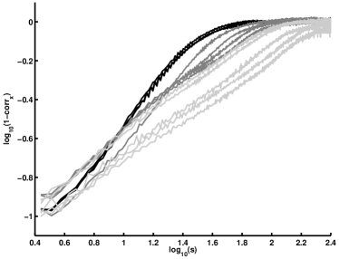
The effects on the correlation functions are shown in Figs. 9 and 10. For clarity, the log of is plotted against the log of the comoving length along the string , which separates the curves so the changes in gradient are more apparent. It is clear from the tangent vector correlations that when the evolution is artificially damped, the small scale structure is quite different. The initial slope for is close to unity, as expected for smooth strings, which is maintained for a short time. Then begins a transition towards a new exponent as scaling is attained for the new undamped (Hubble damping only) evolution. The power law changes first at small scales and moves up to larger scales as the evolution adjusts to the new conditions. Once the exponents have relaxed, the small scale structure behaves and scales just as in an undamped simulation with no recollection of the initial damping conditions.
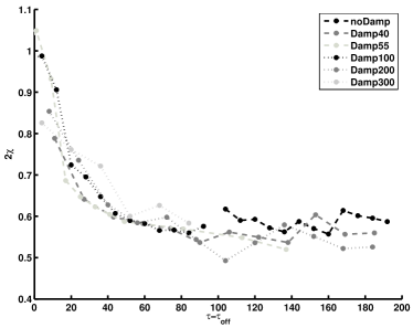
The exponents are found by setting as found for the radiation era simulations on a lattice which are also consistent with that found for a single simulation. So in this case only a 2 parameter fit is made for Eq. (22); and . is found to be constant and consistent in both a damped and undamped evolution so we discuss the relaxation time scale in terms of the time taken for the gradient parameter, , to transition back into scaling. There is little effect on the value of once the new scaling value is reached after damping and becomes approximately 0.6, the same as found during the scaling epoch for a completely undamped simulation. The profile of this relaxation is compared for different damped simulations and shown in Fig. 11.
Although not conclusive, there is evidence that the relaxation time, from the moment damping is turned off , is approximately . One can see the trend most clearly in the value of at . This is explicable if the transition is triggered by intercommutation and the generation of kinks, which would have the observed effect of reducing the correlation at small scales.
Figs. 9 and 10 show the correlators settling into a scaling regime behaving much as the evolution with Hubble damping only. We recall also that the network length scale returns to the expected linear behaviour, Fig. 5, over perhaps an even shorter time frame. We interpret these features as good evidence that calculations can be trusted to not depend on initial conditions.
IV.3 Comoving String Core Width
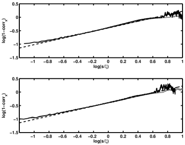
Simulations conducted in the radiation era are possible with the true equations of motion using in Eqs. (8)-(9) and correlation results for an average of simulations for the correlation function results are tested against results. Fig. 12 shows a comparison of the correlations at two different times in the simulation for both the and the cases. The difference in the results is surprisingly insignificant for this calculation and no correction is felt necessary.
IV.4 Testing Gaussianity
The 4-point correlation functions and are also calculated to test for gaussianity.
Denoting each spatial component of as , with some initial base point for the measurement, the fourth moments formula is written
| (25) | |||||
Then gaussianity would allow contraction on all pairs from Wick’s Theorem so that and the ratio of the 4 point functions should behave as
Fig. 13 shows for the radiation era that on all scales the ratio of the 4 point correlations is not constant and not . The 4-point correlators in the matter era (not plotted) behave in a similar way.
In the model for loop production proposed by Polchinski and collaborators Polchinski and Rocha (2006); Dubath et al. (2008); Polchinski and Rocha (2007), it is argued that non-gaussianity does not affect the power laws derived for the 2-point correlation function or the loop production function. We have confirmed that the 2-point correlation function is in accord with their model, but in the next section we will see that the loop production function is not. If we accept the arguments of Polchinski et al, which are based on scaling, another reason must be found to account for the difference.

V Loop Distributions
Loop production in cosmic string networks is still a subject of some debate despite a number of recent numerical investigations using the Nambu-Goto approximation Ringeval et al. (2007); Olum and Vanchurin (2007); Martins and Shellard (2006), taking advantage of improvements in computational facilities and algorithms, and focusing on small scale structure and loop production rates.
The crucial quantities in question are the loop (length) distribution function and the loop production function. Unfortunately, the different groups measure different quantities, and emphasise different features, so the results are difficult to compare.
Those that measure the loop production function Olum and Vanchurin (2007); Martins and Shellard (2006) find that it peaks at a small scale, with a power-law rise Olum and Vanchurin (2007), and a less prominent feature at about a tenth of the horizon length . The identity of the small scale is not clear, but on inspection of the data Martins and Shellard (2006); Olum and Vanchurin (2007), it appears to be related to (and at least no greater than) the initial comoving correlation length. Full scaling requires that the only scale in the distribution and production functions should be : the peak therefore does not scale. Furthermore, it is found that the amplitude of the power law does not scale either Olum and Vanchurin (2007).
Measurements of the loop distribution function on the other hand Ringeval et al. (2007), show a peak at the initial numerical cut-off, and scaling at intermediate scales. The peak is understandable as a transient from the initial evolution, but as the distribution function is essentially the time integral of the production function, the intermediate range scaling is a puzzle.
It has been suggested that the non-scaling of the loop production function is a transient effect Martins and Shellard (2006); Olum and Vanchurin (2007), and that the peak should eventually disappear altogether Olum and Vanchurin (2007) or start scaling if only a large enough simulation could be performed Martins and Shellard (2006). However, the evidence that a power-law with a small-scale cutoff is a real feature of Nambu-Goto string networks has been strengthened thanks to the agreement with Polchinski and collaborators’ model of loop production Polchinski and Rocha (2006, 2007); Dubath et al. (2008). There is also no evidence for scaling of the peak in the loop production function from visual inspection of the graphs in Refs. Martins and Shellard (2006); Olum and Vanchurin (2007).
Accepting the evidence of a power-law form for the loop production function, a small-scale cut-off is required to keep the total energy loss finite. The conventional string scenario demands full scaling, and invokes gravitational radiation reaction to change the loop production scale to a constant fraction of the horizon size, which is , according to Ref. Polchinski and Rocha (2007). However, there are no network simulations including gravitational radiation reaction so this is still a conjecture. It could equally well be that loop production really does not scale as the Nambu-Goto simulations suggest; this does not prevent the energy density of the long string network from scaling. Furthermore, if the small-scale cut-off is the string width Vincent et al. (1997a), it is necessary to perform field theory simulations in order to include the true small-scale physics.
Previous field theory simulations Vincent et al. (1998); Moore et al. (2002) have not studied the loop distributions in any detail, but it is already clear that their properties are very different from the Nambu-Goto versions. The number of loops in the simulation volume is substantially less, which prompted the suggestion Vincent et al. (1998) that the network could lose energy to classical radiation directly rather than via the production and eventual decay of loops. Arguing in favour of loop production, it was pointed out in Moore et al. (2002) that even if all the energy is lost to “core” or “proto”-loops (loops whose length is of order the string width) that the number density would be very low anyway, approximately . It was also conjectured that these core loops would eventually grow if a large enough simulation could be performed.
In the first part of this section we test the hypothesis that a substantial fraction of the energy loss from long strings is in the form of core loops. The impression given by visualisations such as Fig. 1 is that direct radiation appears to be very important, although it is very difficult to tell the difference between a large amplitude excursion by the Higgs field and a core loop. However, if energy loss into core loops is important we would expect to find core loops near long strings, and our first test is to look for these correlations.
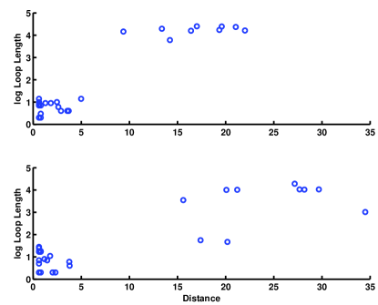
We define a core loop as a loop with the minimum number of lattice segments to create a closed loop (i.e. 4 linked segments, located as described in Sec. III.4). With , the core loop length is approximately the string width. We then measure the distance from core loops to the closest point on a neighbouring piece of string and the length of the string to which it is closest. The results are shown in Fig. 14. Interestingly, it is seen that core loops lie close to other very small loops and that these clusters or isolated core loops lie at distances of order half the correlation length from long string; between two long strings. As loops collapse they appear to fragment into clusters of very small loops but the lack of core loops close to long strings argues against small loop production being a significant source of energy loss from long strings.
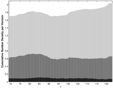
We can also check the hypothesis by looking at the number distribution of loops in field theory simulations, using a large number of runs. The length scales of interest are the string width (core loops) and the network correlation length, , defined as Eq. (11). Fig. 15 shows cumulatively the number densities of loops per horizon in the radiation era over the conformal time range when the network is scaling. The loops are divided into those of length 4 links (core loops), those up to length , and those beyond. Core loops are seen to occupy a constant small fraction of the number density. In each of these classes the number density of loops per horizon appears to be constant. The number of core loops per horizon is very small, of order .
We can estimate whether this is consistent with core loops being a significant channel of energy loss for long strings. If a network with comoving length scale decays into loops of size , then their lifetime should also be , given the shrinking mechanism outlined in Section II. The number of loops per horizon volume should then be . Given that , there are roughly 100 times too few core loops if they were to take a significant amount of energy away from long strings.
Our result seems to be in contradiction to Ref. Moore et al. (2002), who use a fit to the Velocity-dependent One-Scale model Martins and Shellard (1996b) to argue that loop production is significant in their field theory simulations. However, they do not give absolute values of the loop distribution function and so it is not possible to compare the results directly. One possible resolution, explored in more detail below, is that horizon-size loops with lifetime are carrying away an appreciable fraction of the energy.
To study the loop distribution and production functions in more detail, we must model both the production and shrinking of loops. We denote the loop distribution function in terms of the cosmic time and physical length as , where and is the comoving loop length, which is given in terms of the string variables and by . We denote the comoving loop distribution function in conformal time as . Then the number density of loops in physical length interval is related to the comoving number density of loops in interval by
| (26) |
The equation governing the loop distribution function is
| (27) |
where we introduce the loop production function in physical units . We also take into account energy loss from loops which we shall assume takes place at a constant rate such that . We estimate from the properties of the energy loss mechanism outlined in Sec. II333Gravitational radiation would give were it to be included. Using Eq. (26) we can relate the comoving number density distribution and the loop production function in comoving units
| (28) |
where .
Assuming scaling, the comoving loop production function and number density distribution behave as Vilenkin and Shellard (1994)
for functions and of the dimensionless ratio of loop length to horizon size . Rewriting Eq. (28) in terms of and one obtains (with ),
with solution
| (29) |
Numerical simulations suggest a power law for loop production, below . If radiative effects can be neglected (), and making the reasonable assumption that vanishes for , we have from Eq. (29)
| (30) |
For length scales where radiative effects are strong ()
| (31) |
To make our measurement we define the comoving loop number density in a length interval
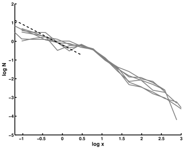
Figs. 16 and 17 show an estimate for
taken from the average of runs in radiation and matter eras respectively. The solid black line in Fig. 16 the the initial loop distribution function which shows good agreement with the expected power law of slope , Vachaspati and Vilenkin (1984).
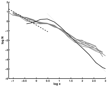
For a network that has reached scaling, the analytic model of Ref. Polchinski and Rocha (2006), further refined by Dubath et al in Dubath et al. (2008), proposes that loop density is dominated by recently produced loops. They derive a function for loop production which they extrapolate to loop number density distribution under the assumption that radiative effects can be ignored and obtain
| (32) |
with defined in Eq. (20). If radiative effects are considered the exponent for the number density distribution function will be higher by at small length scales by the arguments from Eqs. (29) and (31). This is also consistent with the analytic findings of Rocha in Ref. Rocha (2008) where the loop distribution model is enhanced by including of the effects of gravitational radiation. From the values of calculated from our simulation results and given in Table 1, this would give exponents of in the radiation era and in the matter era which are compared to our data in Figs. 16 and 17. The agreement remains less than convincing, particularly for the radiation era.
Olum et al Olum and Vanchurin (2007) calculate the loop production function from their Nambu-Goto simulations. The function drops from a small-scale peak with a power law consistent with the model proposed by Dubath et al Dubath et al. (2008): . The exponent is calculated using Eq. (20) with velocities taken from simulations of Ref. Moore et al. (2002); and . No fit values for the gradient of are quoted in Ref. Olum and Vanchurin (2007) but pictures showing average gradients of their loop production function in the matter and radiation era are used in Ref. Dubath et al. (2008) to demonstrate their model. Exponents are listed in Table 2.
Number densities can also be compared with Nambu-Goto simulations of Ref. Ringeval et al. (2007) who quote a length distribution,
| (33) |
They find a consistent power law over the whole range of their Nambu-Goto simulation with exponents for the radiation dominated era and in the matter era. Given that there is no decay mechanism in Nambu-Goto simulations we can infer slopes for the loop production function of and for radiation and matter eras respectively, in good agreement with the values predicted by the model Dubath et al. (2008) for Nambu-Goto strings. However, even if radiative effects are taken into consideration these results are steeper than those predicted for our Abelian Higgs strings, (see Table 2), which are already too steep to fit our data.
The flatter power law for loop distributions found in the field theory examination Figs. 16 and 17 can be better explained by invoking loop production and fragmentation at horizon scales combined with energy loss at small scales. From Ref. Scherrer and Press (1989) it is predicted that unusual power laws for the production of loops can be explained by loop fragmentation probabilities, , with . For small loops where radiative effects are strong, number density distribution functions will take the form . Then the steepest slope possible would be when the fragmentation probability is of order unity.
We also see evidence of loop production at the horizon scale in the small feature visible in the loop distribution function at , which has some similarity to the Nambu-Goto simulations of Olum and Vanchurin (2007). It is straightforward to check that the production of one such loop per horizon volume per Hubble time is sufficient to remove a significant fraction of the energy in long strings. Given that these loops are losing length at a rate of order 1 as well as fragmenting, this is consistent with our observation of order one loop per horizon volume at any time. The correlation of core loops with other small loops shown Fig. 14 can also be explained by loop fragmentation.
Finally, we note that the large behaviour in our number density analysis remains a puzzle, as it departs from the -2.5 slope expected outside the horizon. It maybe that the loop distribution at these much longer length scales is quite sensitive to the finite volume of the simulation Austin et al. (1994).
| Abelian Higgs Prediction | ||
| Nambu-Goto Prediction | ||
| Nambu-Goto Measurement |
VI Conclusions and Remarks
In this paper we have examined small scale structure, energy loss and loop production in cosmic strings found in the Abelian Higgs model (AH), using numerical simulations, and compared the results to those from Nambu-Goto (NG) simulations in the literature. We have also investigated the energy loss mechanism which causes Abelian Higgs strings to scale without gravitational radiation.
We first studied the two point tangent vector correlation function (Eq. IV.1), for which there is a clear prediction based on the NG equations by Polchinski and Rocha (PR) Polchinski and Rocha (2006). Their model predicts that the correlator scales, i.e. that it is a function of the ratio of distance to the horizon scale, and that this function has a power law form with an exponent determined by the mean square velocity of the string. The correlator is seen to scale very well, and good agreement with the power law is found right down to the string core width scale. The mean square velocity is about in both the radiation and matter eras, markedly lower than in NG simulations ( and and respectively Bennett and Bouchet (1990); Martins and Shellard (2006)). This is likely to be due to back-reaction from the massive radiation.
We test the sensitivity of the tangent vector correlator to the initial conditions by damping the strings for an initial interval of various duration. We see that the network regains its scaling form after a time of approximately . In this relaxation period we see evidence that the build up of small scale structure appears to move from small scales to large. It is plausible that the trigger for the production of small scale structure and the relaxation of scaling is intercommutation of long strings. The fact that the structure appears bottom-up argues against small-scale structure being due to residual power from the Brownian random walk at super-horizon scales, as argued in Polchinski and Rocha (2006).
The small scale structure seen in the tangent vector correlations can help to explain the scale separation problem described in Sec. II, which is to understand how massive radiation of frequency around about the string width is produced from fields which are apparently changing with a frequency of about the Hubble rate. The solution is that if strings are not smooth on small scales, the radius of curvature at these scales is much smaller and frequency of modes of oscillations of the string much higher than the Hubble rate.
The PR model also has key predictions for loop production Polchinski and Rocha (2006); Dubath et al. (2008), and shows how the small-scale structure accounts for the production of loops at the small-scale cutoff in Nambu-Goto (NG) simulations. We were therefore led to investigate loop distributions in AH simulations also, and to try to connect small scale structure and energy loss in our field theory simulations by looking for core (string width sized) loops.
We found that the model for loop production in Ref. Dubath et al. (2008) does not describe loop distributions in AH simulations, disagreeing with the observed power law. Furthermore, a lack of spatial correlation between core loops and long string, and a very low overall number density, roughly 0.1 per horizon volume, point towards there being no significant energy loss through direct production of core loops from long string.
Our results support the statement that significant energy is lost directly from AH strings. This can be seen in snapshots from field theory simulations (Fig. 1) with long string radiating energy directly into oscillations of the field as Higgs and gauge radiation. Our results also indicate that larger loops share this rapid energy-loss mechanism, which therefore needs to be added to the the standard model for loop distributions. We make a simple modification, that energy is radiated from loops at a constant rate. When coupled with an alternative model of loop production Scherrer and Press (1989), which proposes fragmentation of horizon-sized loops, we are able to explain our results for the loop distribution.
As an aside, a feature of the calculation for the loop distribution function in Ref. Dubath et al. (2008) is that the string correlators are assumed to be Gaussian, although it is argued that this is not crucial to the form of the result. The four point correlation in our simulations is explicitly non-Gaussian, but does scale.
So when gravity can be neglected a general picture for the evolution of cosmic string networks is developing. A dominant energy loss mechanism works at the small-scale cutoff, which is loop production in NG simulations and classical radiation in the field theory. Energy is transported from the horizon scale by small-scale structure. In both kinds of simulation loops are produced at the horizon scale, which then fragment with high probability. There is evidence of a population of non-intersecting loops remaining stable in NG Olum and Vanchurin (2007), but in AH, where massive radiation is available, loops radiate and shrink.
We note that the small loops in NG simulations behave like particles with mass , which have similar average energy-momentum properties to classical massive radiation. Thus the striking visual dissimilarity of NG and AH simulations is perhaps misleading: if one interprets the small loops as representing massive radiation and concentrates on the long string network, the differences are greatly reduced. It is interesting to speculate that the small loops might really be massive states for fundamental cosmic strings.
It remains a bit of a puzzle why AH strings have a highly suppressed production of small loops. The PR prediction, based on the NG equations of motion, is that small loop production should be dominated by the smallest physical scale, which for AH simulations is the string width, but few are observed. As the NG equations of motion break down at the string width scale, it is perhaps not surprising to see the break-down of a prediction based on those equations.
In the traditional cosmic string scenario it is assumed that gravitational radiation back reaction plays a vital role in smoothing long strings, disguising the small-scale physics of the strings, and setting the scale for loop production. In this scenario most of the energy ends up as long-wavelength gravitational radiation, as opposed to ultra-high energy particles Vincent et al. (1997a); Vincent et al. (1998).
It is by no means obvious that gravitational radiation reaction is strong enough to shut off the efficient and rapidly established energy loss mechanism afforded by massive radiation in a field theory. Our simulations show that it is not necessary to postulate gravitational radiation reaction to achieve scaling and a consistent picture of string network evolution. Nonetheless, it is still possible that gravitational radiation could operate as traditionally supposed. As a first step, we intend to test the impact of massless radiation on string network evolution with an investigation of small scale structure and loop distributions in field theories that have massless degrees of freedom, for instance global strings, and the Abelian Higgs model coupled to a dilaton.
Acknowledgements.
Simulations were performed using the COSMOS Altix 3700 supercomputer (supported by SGI/Intel, HEFCE, and STFC) and the University of Sussex HPC Archimedes cluster (supported by HEFCE). We acknowledge financial support from STFC. We thank Ed Copeland, Tom Kibble, Carlos Martins, Ken Olum, Christophe Ringeval, Mairi Sakellariadou and Tanmay Vaspachi for useful discussions.References
- Polchinski and Rocha (2006) J. Polchinski and J. V. Rocha, Phys. Rev. D74, 083504 (2006), eprint hep-ph/0606205.
- Dubath et al. (2008) F. Dubath, J. Polchinski, and J. V. Rocha, Phys. Rev. D77, 123528 (2008), eprint arXiv:0711.0994 [astro-ph].
- Scherrer and Press (1989) R. J. Scherrer and W. H. Press, Phys. Rev. D39, 371 (1989).
- Hindmarsh and Kibble (1995) M. B. Hindmarsh and T. W. B. Kibble, Reports on Progress in Physics 58, 477 (1995), URL http://stacks.iop.org/0034-4885/58/477.
- Vilenkin and Shellard (1994) A. Vilenkin and E. P. Shellard, Cosmic Strings and Other Topological Defects (Cambridge: Cambridge University Press, 1994).
- Sakellariadou (2007) M. Sakellariadou, Lect. Notes Phys. 718, 247 (2007), eprint hep-th/0602276.
- Kibble (1976) T. W. B. Kibble, J. Phys. A9, 1387 (1976).
- Copeland et al. (2004) E. J. Copeland, R. C. Myers, and J. Polchinski, JHEP 06, 013 (2004), eprint hep-th/0312067.
- Yokoyama (1989) J. Yokoyama, Phys. Rev. Lett. 63, 712 (1989).
- Kofman et al. (1994) L. Kofman, A. D. Linde, and A. A. Starobinsky, Phys. Rev. Lett. 73, 3195 (1994), eprint hep-th/9405187.
- Copeland et al. (1994) E. J. Copeland, A. R. Liddle, D. H. Lyth, E. D. Stewart, and D. Wands, Phys. Rev. D49, 6410 (1994), eprint astro-ph/9401011.
- Sarangi and Tye (2002) S. Sarangi and S. H. H. Tye, Phys. Lett. B536, 185 (2002), eprint hep-th/0204074.
- Dvali and Vilenkin (2004) G. Dvali and A. Vilenkin, JCAP 0403, 010 (2004), eprint hep-th/0312007.
- Battye et al. (2006) R. A. Battye, B. Garbrecht, and A. Moss, JCAP 0609, 007 (2006), eprint astro-ph/0607339.
- Bevis et al. (2008) N. Bevis, M. Hindmarsh, M. Kunz, and J. Urrestilla, Phys. Rev. Lett. 100, 021301 (2008), eprint astro-ph/0702223.
- Bevis et al. (2004) N. Bevis, M. Hindmarsh, and M. Kunz, Phys. Rev. D70, 043508 (2004), eprint astro-ph/0403029.
- Wyman et al. (2005) M. Wyman, L. Pogosian, and I. Wasserman, Phys. Rev. D72, 023513 (2005), eprint astro-ph/0503364.
- Fraisse (2007) A. A. Fraisse, JCAP 0703, 008 (2007), eprint astro-ph/0603589.
- Battye et al. (2008) R. A. Battye, B. Garbrecht, A. Moss, and H. Stoica, JCAP 0801, 020 (2008), eprint arXiv:0710.1541 [astro-ph].
- Urrestilla et al. (2008) J. Urrestilla, N. Bevis, M. Hindmarsh, M. Kunz, and A. R. Liddle, JCAP 0807, 010 (2008), eprint arXiv:0711.1842 [astro-ph].
- Fraisse et al. (2007) A. A. Fraisse, C. Ringeval, D. N. Spergel, and F. R. Bouchet (2007), eprint arXiv:0708.1162 [astro-ph].
- Pogosian et al. (2008) L. Pogosian, S. H. H. Tye, I. Wasserman, and M. Wyman (2008), eprint arXiv: 0804.0810 [astro-ph].
- Bevis et al. (2007a) N. Bevis, M. Hindmarsh, M. Kunz, and J. Urrestilla, Phys. Rev. D76, 043005 (2007a), eprint arXiv:0704.3800 [astro-ph].
- Pogosian and Wyman (2008) L. Pogosian and M. Wyman, Phys. Rev. D77, 083509 (2008), eprint arXiv:0711.0747 [astro-ph].
- Kibble (1980) T. W. B. Kibble, Phys. Rept. 67, 183 (1980).
- Vilenkin (1981) A. Vilenkin, Phys. Rev. D24, 2082 (1981).
- Albrecht and Turok (1989) A. Albrecht and N. Turok, Phys. Rev. D 40, 973 (1989).
- Bennett and Bouchet (1990) D. P. Bennett and F. R. Bouchet, Phys. Rev. D41, 2408 (1990).
- Allen and Shellard (1990) B. Allen and E. P. S. Shellard, Phys. Rev. Lett. 64, 119 (1990).
- Vincent et al. (1997a) G. R. Vincent, M. Hindmarsh, and M. Sakellariadou, Phys. Rev. D56, 637 (1997a), eprint astro-ph/9612135.
- Borsanyi and Hindmarsh (2008) S. Borsanyi and M. Hindmarsh, Phys. Rev. D77, 045022 (2008), eprint arXiv:0712.0300 [hep-ph].
- Vincent et al. (1998) G. Vincent, N. D. Antunes, and M. Hindmarsh, Phys. Rev. Lett. 80, 2277 (1998).
- Moore et al. (2002) J. N. Moore, E. P. S. Shellard, and C. J. A. P. Martins, Phys. Rev. D65, 023503 (2002), eprint hep-ph/0107171.
- Everett (1981) A. E. Everett, Phys. Rev. D24, 858 (1981).
- Olum and Blanco-Pillado (2000) K. D. Olum and J. J. Blanco-Pillado, Phys. Rev. Lett. 84, 4288 (2000).
- Bevis et al. (2007b) N. Bevis, M. Hindmarsh, M. Kunz, and J. Urrestilla, Phys. Rev. D75, 065015 (2007b), eprint astro-ph/0605018.
- Polchinski and Rocha (2007) J. Polchinski and J. V. Rocha, Phys. Rev. D75, 123503 (2007), eprint gr-qc/0702055.
- Hindmarsh (1990) M. Hindmarsh, Phys. Lett. B251, 28 (1990).
- Quashnock and Spergel (1990) J. M. Quashnock and D. N. Spergel, Phys. Rev. D42, 2505 (1990).
- Srednicki and Theisen (1987) M. Srednicki and S. Theisen, Phys. Rev. Lett. B 189 p. 379 (1987).
- Brandenberger (1987) R. Brandenberger, Nucl. Phys. B 84, 812 (1987).
- Blanco-Pillado and Olum (1999) J. J. Blanco-Pillado and K. D. Olum, Phys. Rev. D59, 063508 (1999), eprint gr-qc/9810005.
- Weinberg (1972) S. Weinberg, Gravitation and Cosmology (New York: Wiley, 1972).
- Vachaspati and Vilenkin (1985) T. Vachaspati and A. Vilenkin, Phys. Rev. D31, 3052 (1985).
- Damour and Vilenkin (2000) T. Damour and A. Vilenkin, Phys. Rev. Lett. 85, 3761 (2000), eprint gr-qc/0004075.
- Damour and Vilenkin (2001) T. Damour and A. Vilenkin, Phys. Rev. D64, 064008 (2001), eprint gr-qc/0104026.
- Siemens and Olum (2001) X. Siemens and K. D. Olum, Nucl. Phys. B611, 125 (2001), eprint gr-qc/0104085.
- Siemens and Olum (2003a) X. Siemens and K. D. Olum, Physical Review D (Particles, Fields, Gravitation, and Cosmology) 68, 085017 (pages 8) (2003a), URL http://link.aps.org/abstract/PRD/v68/e085017.
- Siemens and Olum (2003b) X. Siemens and K. D. Olum, Phys. Rev. D68, 085017 (2003b), eprint gr-qc/0307113.
- Ringeval et al. (2007) C. Ringeval, M. Sakellariadou, and F. Bouchet, JCAP 0702, 023 (2007), eprint astro-ph/0511646.
- Martins and Shellard (2006) C. J. A. P. Martins and E. P. S. Shellard, Physical Review D (Particles, Fields, Gravitation, and Cosmology) 73, 043515 (pages 6) (2006), URL http://link.aps.org/abstract/PRD/v73/e043515.
- Olum and Vanchurin (2007) K. D. Olum and V. Vanchurin, Phys. Rev. D75, 063521 (2007), eprint astro-ph/0610419.
- Nielsen and Olesen (1973) H. B. Nielsen and P. Olesen, Nucl. Phys. B61, 45 (1973).
- Moriarty et al. (1988) K. J. M. Moriarty, E. Myers, and C. Rebbi, Phys. Lett. B207, 411 (1988).
- Bogomol’nyi (1976) E. Bogomol’nyi, Sov. J. Nucl. Phys. 24, 449 (1976).
- (56) UK National Cosmology Supercomputer: SGI Altix 3700 containing 152 Intel Itanium II CPUs, URL www.damtp.cam.ac.uk/cosmos/.
- (57) N. Bevis and M. Hindmarsh, URL www.latfield.org.
- Kajantie et al. (1998) K. Kajantie, M. Karjalainen, M. Laine, J. Peisa, and A. Rajantie, Phys. Lett. B428, 334 (1998), eprint hep-ph/9803367.
- Bevis and Saffin (2008) N. Bevis and P. M. Saffin, Phys. Rev. D78, 023503 (2008), eprint arXiv: 0804.0200 [hep-th].
- Scherrer and Vilenkin (1998) R. J. Scherrer and A. Vilenkin, Phys. Rev. D58, 103501 (1998), eprint hep-ph/9709498.
- Vincent et al. (1997b) G. R. Vincent, M. Hindmarsh, and M. Sakellariadou, Phys. Rev. D 55, 573 (1997b).
- Martins and Shellard (1996a) C. J. A. P. Martins and E. P. S. Shellard, Phys. Rev. D53, 575 (1996a), eprint hep-ph/9507335.
- Martins and Shellard (1996b) C. J. A. P. Martins and E. P. S. Shellard, Phys. Rev. D 54, 2535 (1996b).
- Vachaspati and Vilenkin (1984) T. Vachaspati and A. Vilenkin, Phys. Rev. D30, 2036 (1984).
- Rocha (2008) J. V. Rocha, Phys. Rev. Lett. 100, 071601 (2008), eprint arXiv:0709.3284 [gr-qc].
- Austin et al. (1994) D. Austin, E. J. Copeland, and R. J. Rivers, Phys. Rev. D49, 4089 (1994).