Quantum quenches from integrability:
the fermionic pairing model

Abstract

Understanding the non-equilibrium dynamics of extended quantum systems after the trigger of a sudden, global perturbation (quench) represents a daunting challenge, especially in the presence of interactions. The main difficulties stem from both the vanishing time scale of the quench event, which can thus create arbitrarily high energy modes, and its non-local nature, which curtails the utility of local excitation bases. We here show that nonperturbative methods based on integrability can prove sufficiently powerful to completely characterize quantum quenches: we illustrate this using a model of fermions with pairing interactions (Richardson’s model). The effects of simple (and multiple) quenches on the dynamics of various important observables are discussed. Many of the features we find are expected to be universal to all kinds of quench situations in atomic physics and condensed matter.

The experimental realization exp of cold atomic systems with a high degree of tunability of Hamiltonian parameters, and the ability to evolve in time with negligible dissipation, has reignited the study of many-body quantum systems away from equilibrium. How Gibbs or any other relaxed states can ultimately result from unitary dynamics is a question that has received a lot of attention recently th-mix ; cc-06 ; gdlp-07 ; IS ; s08 , but which still lacks a general understanding.

Suppose an extended quantum system is prepared in one eigenstate $|\psi_{g_{0}}^{\mu}\rangle$ of some Hamiltonian $H_{g_{0}}$, where $g_{0}$ is a tunable, global parameter (interaction strength, external field, …). At a given time, say $t=0$, this parameter is suddenly changed to a different value $g$, and the system thus starts evolving unitarily according to the dynamics governed by a different Hamiltonian $H_{g}$. This is what is referred to as a quantum quench. The resulting time evolution is simply given by the solution of the Schrödinger equation $|\psi(t)\rangle=e^{-iH_{g}t}|\psi_{g_{0}}^{\mu}\rangle$. Since $|\psi_{g_{0}}^{\mu}\rangle$ is not an eigenstate of $H_{g}$, this can be extremely difficult to quantify. The most straightforward way to tackle the problem is therefore to write the initial state $|\psi_{g_{0}}^{\mu}\rangle$ as a sum over the complete set of eigenstates $|\psi_{g}^{\nu}\rangle$ (having energy $\omega_{g}^{\nu}$) of Hamiltonian $H_{g}$, leading to the time-dependent post-quench state

$$|\psi(t)\rangle=\sum_{\nu}e^{-i\omega_{g}^{\nu}t}\langle\psi_{g}^{\nu}|\psi_{g_{0}}^{\mu}\rangle|\psi_{g}^{\nu}\rangle\,.$$ (1)

The complexity of the problem is encoded first in the distribution of energies $\omega^{\nu}_{g}$, but most importantly in the matrix of overlaps of eigenstates pertaining to the two different Hamiltonians,

$$Q_{gg_{0}}^{\nu\mu}\equiv\left<\psi^{\nu}_{g}|\psi^{\mu}_{g_{0}}\right>\,,$$ (2)

which we call the quench matrix. This matrix is of dimension equal to that of the Hilbert space , but in practice we mainly need a single column expressing the initial eigenstate of $H_{g_{0}}$ in terms of the eigenstates of $H_{g}$. However, even in the very few cases when all eigenstates of a many-body Hamiltonian can be classified and written down, the calculation of the quench matrix coefficients is a severe challenge, whose computational complexity generally grows factorially with system size. Shortcuts can be found for systems having a representation in terms of free particles (like the 1D Ising chains IS ; s08 ) where Wick’s theorem suffices to calculate all the overlaps, but for truly interacting systems this remains a very ambitious programme. Most of the theoretical work on quantum quenches has up to now concentrated on the calculation of correlation functions in specific regimes th-mix ; cc-06 , with little reference to the post-quench state of the system.

Besides describing the state resulting from a quench of state $\mu$, it is also important to be able to characterize the time dependence of physical observables $O$ after the quench. Formally, we can write

$$\left<O(t)\right> \equiv \langle\Psi(t)|O|\Psi(t)\rangle$$ (3)

$$= \sum_{\nu,\xi}e^{i(\omega_{g}^{\nu}-\omega_{g}^{\xi})t}Q_{g_{0}g}^{\mu\nu}Q_{gg_{0}}^{\xi\mu}\left<\psi^{\nu}_{g}\right|O\left|\psi^{\xi}_{g}\right>\,,$$

where calculating the matrix elements $\left<\psi^{\nu}_{g}\right|O\left|\psi^{\xi}_{g}\right>$ represents an additional hurdle for interesting observables in nontrivially interacting models. Even if we are able to obtain these matrix elements, the leftover double sum over the full Hilbert space is enormous, and one can wonder whether this way of proceeding is of any practical use. New nonperturbative methods are clearly needed to obtain a proper description of the physics involved.

The purpose of the present paper is to introduce a new line of attack on quantum quench problems, sufficiently powerful to yield not only the quench matrix of specific interacting problems (and thus the ensuing nonequilibrium state), but also able to provide matrix elements of physical observables, and thus their time dependence after the quench. This approach is based on the exact solvability of certain many-body quantum problems known as integrable or Bethe Ansatz BetheZP71 solvable theories. Integrability came into prominence as a means of obtaining exact results for the equilibrium thermodynamics of one-dimensional systems (see KorepinBOOK ; TakahashiBOOK and references therein). More recently, a description of correlation functions at equilibrium has been achieved by exploiting results from the Algebraic Bethe Ansatz (ABA), which provides economical expressions for matrix elements of local operators in the basis of exact Bethe eigenstates. The existence of these expressions stems from two results: Slavnov’s formula s-89 for the overlap of a Bethe state with a generic state, and the solution of the so-called quantum inverse problem KitanineNPB554 , i.e. the mapping of physical operators to ABA operators. These matrix elements are of great utility in the computation of equilibrium correlation functions. One very important feature is that Bethe states typically offer a very optimized basis in which only a very small minority of eigenstates carry substantial correlation weight, allowing the summation over intermediate states to be drastically truncated without significantly affecting the results. This novel approach has been successfully applied to equilibrium correlations of quantum spin chains cm-05 and atomic Bose gases cc-06b . We here further extend the reach of integrability into the domain of non-equilibrium quench dynamics.

THE MODEL AND ITS SOLUTION

We consider a model of spin $1/2$ fermions in a shell of energy levels $\epsilon_{\alpha}$ with a Cooper pairing-like interaction

$$H=\sum_{\alpha}\sum_{\sigma}\frac{\epsilon_{\alpha}}{2}c^{\dagger}_{\alpha\sigma}c_{\alpha\sigma}-g\sum_{\alpha,\beta}c^{\dagger}_{\alpha+}c^{\dagger}_{\alpha-}c_{\beta-}c_{\beta+}\,,$$ (4)

which was introduced by Richardson rs-62 in the context of nuclear physics, and has found applications in the physics of ultrasmall metallic grains rev . It reduces to conventional Bardeen-Cooper-Schrieffer (BCS) theory bcs-57 in the thermodynamic (TD) limit. The model has a pseudo-spin representation with $S^{-}_{\alpha}=c_{\alpha\downarrow}c_{\alpha\uparrow}$ (see Methods) with $N$ spins. Central to our approach is the fact that this Hamiltonian can be diagonalized using the Bethe Ansatz rev ; zlmg-02 . The Hilbert space separates into sectors of fixed number of down spins $N_{r}$. The eigenstates of the model are given by Bethe wavefunctions, each individually characterized by a set of $N_{r}$ rapidities $\{w_{j}\}$ obeying a set of algebraic equations known as the Richardson equations

$$\frac{1}{g}=\sum_{\alpha=1}^{N}\frac{1}{w_{j}-\epsilon_{\alpha}}-\sum_{k\neq j}^{N_{r}}\frac{2}{w_{j}-w_{k}}\,\quad j=1,\dots,N_{r}\,,$$ (5)

and are obtained by repeated action of an operator $B(w_{j})$ on the fully polarized reference state $|0\rangle$:

$$|\{w_{j}\}\rangle=\prod_{j}B(w_{j})|0\rangle=\prod_{k=1}^{N_{r}}\sum_{\alpha=1}^{N}\frac{S_{\alpha}^{-}}{w_{k}-\epsilon_{\alpha}}|0\rangle.$$ (6)

The $\binom{N}{N_{r}}$ different solutions to (5) then allow to construct a full set of orthogonal eigenstates, providing us with a proper basis of the Hilbert space.

In Bethe Ansatz solvable models, Slavnov’s formula s-89 , gives the overlap of an eigenstate $|\{w\}\rangle$ with a general Bethe state $|\{v\}\rangle$ (see Methods). The main difference with other models solvable by Algebraic Bethe Ansatz (like the one-dimensional Bose gas or the XXZ chain) is that in the definition of the eigenstates (6), the coupling constant $g$ enters only implicitly through the solutions of the Richardson equation for $w_{j}$. Consequently, for this model, Slavnov’s formula is enough to calculate the overlaps between two generic states at any coupling. For other models, where $B(w_{j})$ depends explicitely on $g$, it can only be used between states defined by the same operators $B(w_{j})$ and therefore the same $g$, and a more general expression for the overlaps remains to be found.

We can then exploit the accessibility to the quench matrix for the Richardson model to show how useful integrability can be when studying quenches. However, before entering in the details of the quantum dynamics, it is important to remember that in the TD limit $N_{r},N\to\infty$ at fixed filling, the dynamics becomes classical bl-06 ; bcs because of suppression of quantum fluctuations. In this limit, the dynamics of the canonical order parameter can be obtained analytically by exploiting classical integrability bl-06 ; bcs . The framework we propose in this letter works in the mesoscopic regime (finite $N$), allowing to study the effects of quantum fluctuations. With this tool at hand, we can characterize in an exact manner the crossover taking place between microscopic and macroscopic physics, a task impossible to achieve with thermodynamical approaches.

We will argue in the following that, similarly to what is observed for equilibrium correlation functions, only a relatively small set of states contributes significantly to the decomposition of the initial state in the new eigenbasis. The natural approach is then to truncate in an optimal way the Hilbert space, so that a faithful representation of the initial state is obtained. The induced truncation error is easily evaluated looking at how close $\sum_{\mu}\left|\langle\psi_{g_{0}}^{0}|\psi_{g}^{\mu}\rangle\right|^{2}$ is to the desired value of $1$. Using the truncated Hilbert space we can then calculate any observable or correlation function by brute force summing the relevant contributions.

Compared to other numerical truncation methods, this approach has the great advantage that time enters only as a parameter. The explicit expression (1) for the wavefunction means that at any time, expectation values can be computed without knowing the previous history of the system (apart from the initial state) and there is therefore no accumulation of errors as time passes. On the other hand, compared to numerical exact diagonalization, matrix elements can be expressed using Slavnov’s formula as matrix determinants whose computational complexity is algebraic and not exponential in the system size and/or number of excitations, thereby allowing to reach large system sizes.

NUMERICAL RESULTS

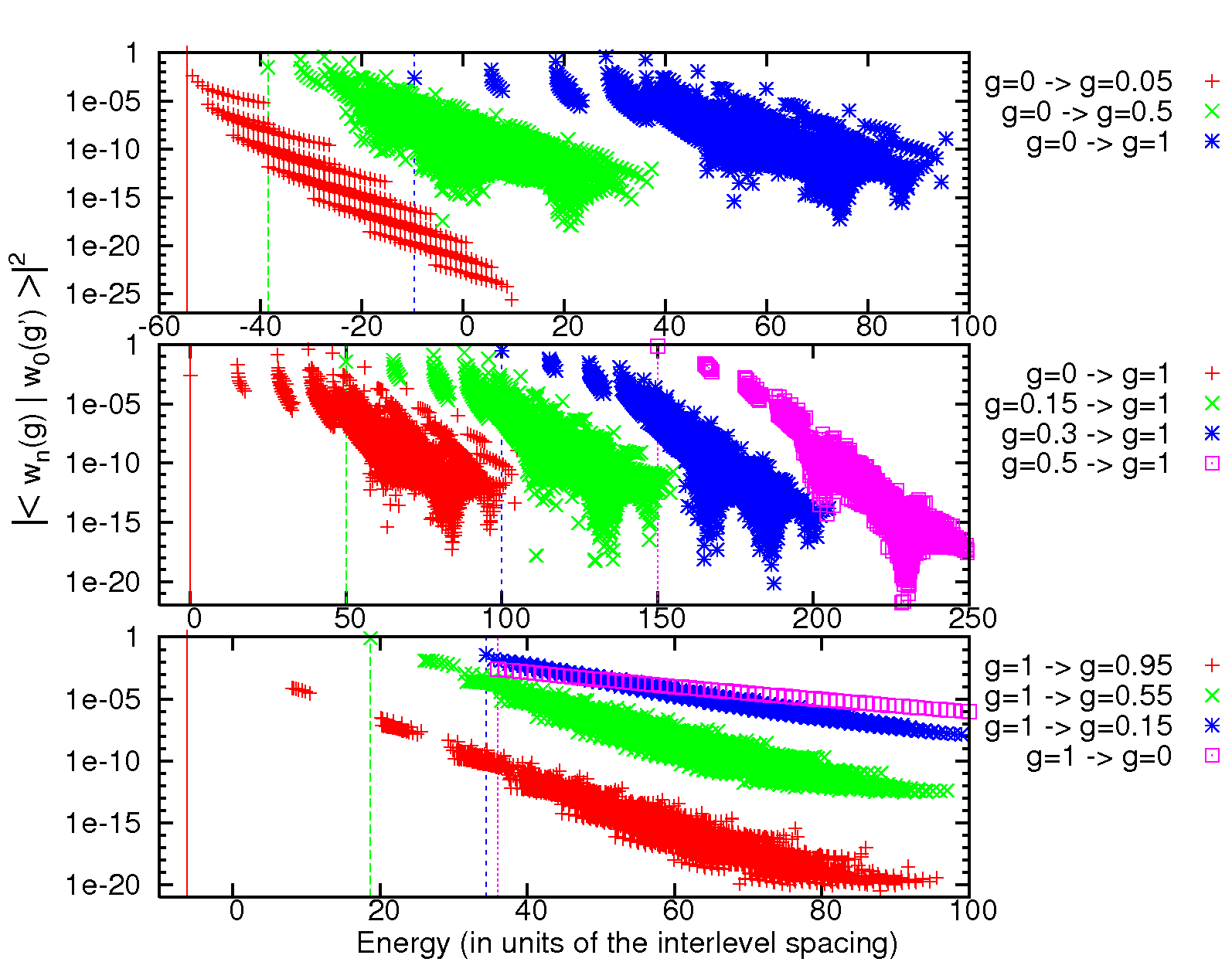
Figure 1: First column of the quench matrix (ground-state overlaps) for several quenches. In all plots $N=2N_{r}=16$ and the ground state energies (represented by vertical lines) have been shifted for clarity. Top: Decomposition of the $g=0$ ground-state with states at $g=0.05,0.5,0.95$. Center: Decomposition of several initial ground-state $g_{0}=0,0.15,0.3,0.5$ in terms of the states at $g=1$. Bottom: Decomposition of the $g_{0}=1$ ground-state in terms of $g=0.95,0.55,0.15,0$ states.

Let us now report explicit results starting with the quench matrix itself. We concentrate on the case of equally spaced levels $\epsilon_{\alpha}$ at half-filling, but the method is clearly not limited to this case. Let us start from $N=2N_{r}=16$, when the Hilbert space has a dimension of “only” 12870. We can then numerically compute the rapidities for every single state. We report in Fig. 1 the square of the overlaps for several quenches as obtained from Slavnov’s formula (see Methods). Starting from the non-interacting ($g=0$) ground state, the top inset shows the overlaps with all the states at three different finite couplings. This allows to understand some general features: having access to the complete quench matrix, one realizes that only a few of the eigenstates at coupling $g$ have a large contribution to $|\psi_{0}\rangle$. Therefore, getting a nearly exact description of the dynamics requires only a small subset of the states. The final state having the largest overlap with the initial ground state is always one of the states that at $g=0$ is built by flipping from up (down) to down (up) the $N_{p}$ spins right below (above) the Fermi level. We refer to these $N_{r}+1$ states as ‘single block states’. For the cases we studied here, quenching from a non-interacting initial state, these states always contribute more than $60\%$ of the total amplitude (see Fig. 2). The total contribution of single block states is non-monotonic in $g$ showing (after decline at small interaction) a rise as $g$ gets sufficiently large.

The ‘band-like’ structure of the overlaps in Fig. 1 makes it reasonable to assume that additional large contributions can be found for states built by slightly deforming the single block ones, e.g. by adding a single particle-hole excitation either above or below the Fermi level. The remaining most relevant states will then be those with two additional excitations. Following this assumption inductively, we add to the truncated Hilbert space multiple block states obtained by slightly deforming single block ones. This allows us to describe larger systems while retaining a tractable number of states. This procedure works extremely well, e.g. at $N=32$, for all the quenches from $g_{0}=0$ to $g\in(0,1]$, we were always able to find at minimum $97\%$ of the weight of the initial state by using only 7000 states, i.e. only $1/10^{5}$ of the full Hilbert space. Moreover, for a given final value of $g$, less than a 1000 of these states gives an actual important contribution.

$$\bullet\bullet\bullet\bullet\bullet\bullet|\circ\circ\circ\circ\circ\circ$$

$$\bullet\bullet\bullet\bullet\bullet\circ|\bullet\circ\circ\circ\circ\circ$$

$$\bullet\bullet\bullet\bullet\circ\circ|\bullet\bullet\circ\circ\circ\circ$$

$$\bullet\bullet\bullet\circ\circ\circ|\bullet\bullet\bullet\circ\circ\circ$$

$$\bullet\bullet\circ\circ\circ\circ|\bullet\bullet\bullet\bullet\circ\circ$$

$$\bullet\circ\circ\circ\circ\circ|\bullet\bullet\bullet\bullet\bullet\circ$$

$$\circ\circ\circ\circ\circ\circ|\bullet\bullet\bullet\bullet\bullet\bullet$$

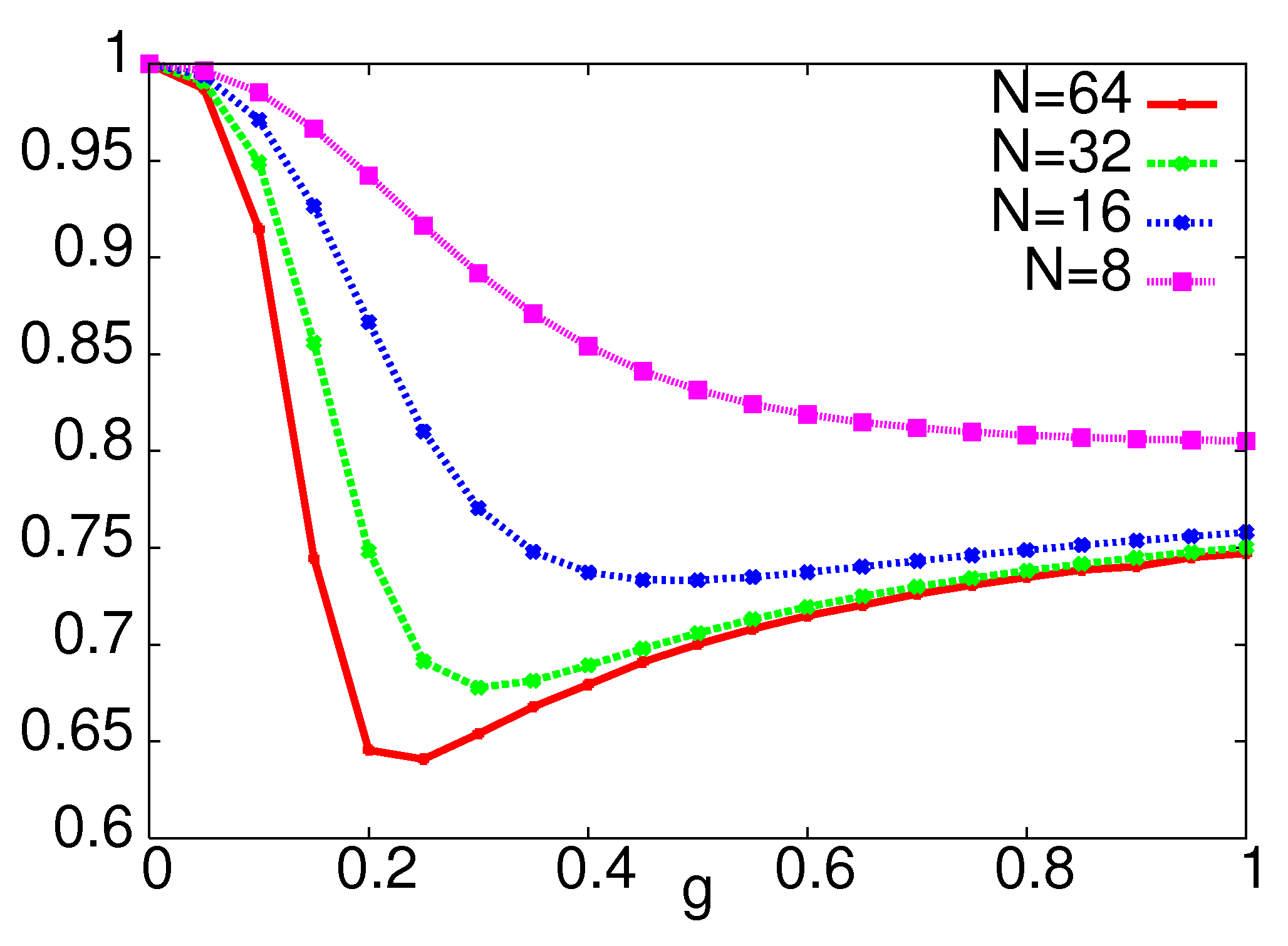
Figure 2: Left: Pictorial representation of single block states obtained by promoting contiguous blocks of $N_{p}\leq N_{r}$ rapidities from right below to right above the Fermi level. Right: Total contribution of these states to the amplitude of the initial state at $g_{0}=0$, as a function of interaction.

In the center of Fig. 1, we report the overlaps obtained by quenching from different initial values of $g_{0}$ to the same final $g=1$. We see that the same band-like structure is present as when starting from a non-interacting state, leading to no qualitative change of the dynamics. Vice-versa, the structure of the quench matrix for a reversed quench, i.e. from large to small $g$, reported in the bottom of Fig. 1 is different: the weight of the state goes down exponentially with the energy of the states (almost straight lines in the figure), and for large quenches the decay rate in energy is slow. An adequate representation of the initial state therefore requires that lots of states be taken into account. In this case, the optimal truncation procedure is still easily defined by simply keeping a sufficient number of low energy states.

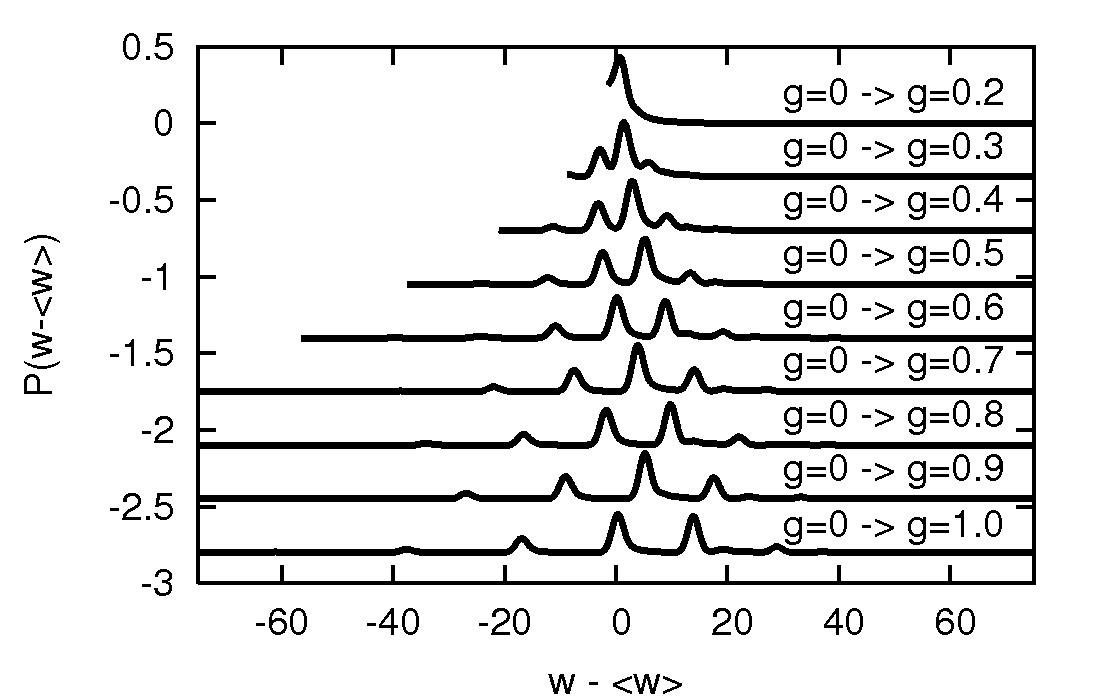
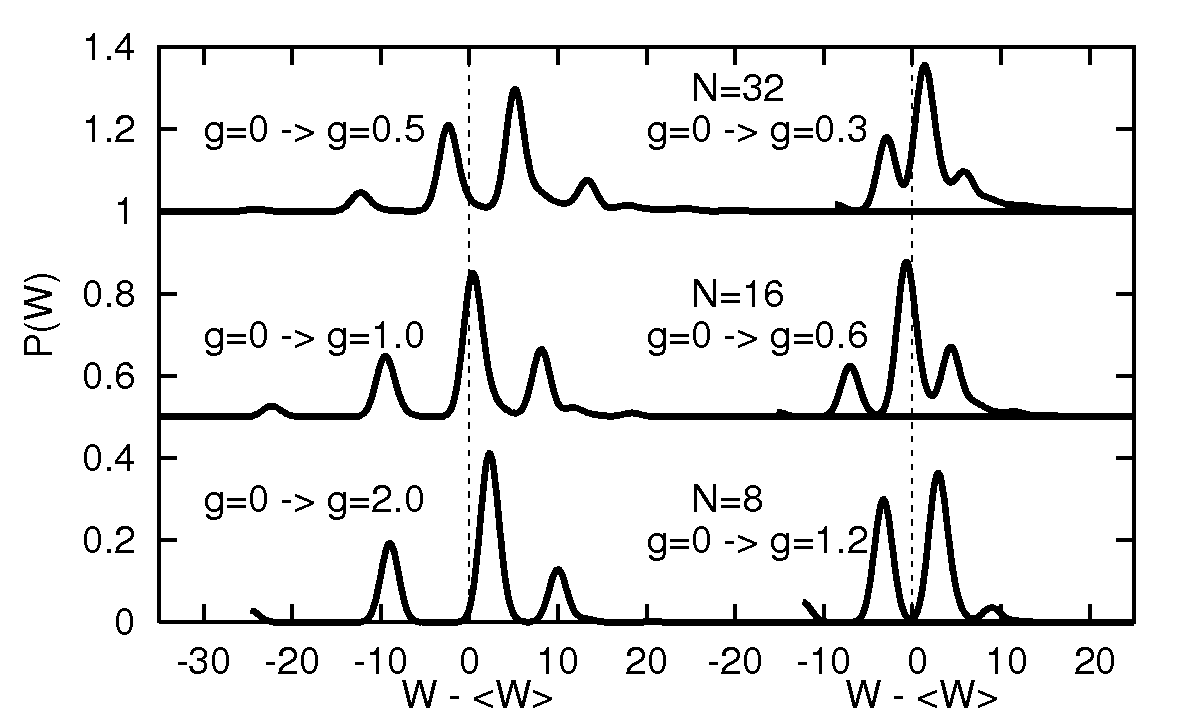
Figure 3: Distribution of work $P(W)$. Top: Different quenches at fixed $N=32$, showing the formation of multiple peaks for large quenches. Bottom: At different $N$ keeping fixed $gN$.

The first measurable quantity easy to derive from the knowledge of the quench matrix is the probability distribution of the ‘work’ s08

$$P(W)=\sum_{\mu}|\langle\psi_{g_{0}}^{0}|\psi_{g}^{\mu}\rangle|^{2}\delta(W-\omega_{g}^{\mu}+\omega_{g_{0}}^{0})\,,$$ (7)

reported for some quenches from $g_{0}=0$ in Fig. 3. These figures have been obtained by smoothing the $\delta$ function with a Gaussian of width proportional to the inter-level spacing. It is straightforward to derive the average and the width of this distribution

$$\langle W\rangle = \langle\psi_{g_{0}}^{0}|(H_{g}-H_{g_{0}})|\psi_{g_{0}}^{0}\rangle=(g_{0}-g)N_{r}\Psi_{OD}^{g_{0}}\,,$$ (8)

$$\langle W^{2}\rangle = \langle\psi_{g_{0}}^{0}|(H_{g}-H_{g_{0}})^{2}|\psi_{g_{0}}^{0}\rangle=(g_{0}-g)^{2}N_{r}^{2}\Psi_{2}^{g_{0}}\,,$$

where $\Psi_{OD}^{g_{0}}=\langle\psi_{g_{0}}^{0}|(\sum^{N}_{\alpha,\beta=1}S^{+}_{\alpha}S^{-}_{\beta})/N_{r}|\psi_{g_{0}}^{0}\rangle$ is the off-diagonal order-parameter in the initial state, and $\Psi_{2}^{g_{0}}=\langle\psi_{g_{0}}^{0}|(\sum^{N}_{\alpha,\beta=1}S^{+}_{\alpha}S^{-}_{\beta}/N_{r})^{2}|\psi_{g_{0}}^{0}\rangle$ is a four point correlator. Higher cumulants are similarly obtained and only depend on the initial state . From TD relations s08 , it is generically expected that the probability of work per spin $w=W/N$ becomes a delta function. For finite $N$, $P(W)$ is non-trivial: it shows a dominant peak close to $W=\langle W\rangle$, but with a structure dictated by the presence of the state with the right quantum numbers at the given energy. In the top panel we report several quenches at $N=32$, where the formation of subdominant peaks is explictly shown. In the bottom panel we show $P(W)$ at different $N$ keeping $gN$ fixed. It is evident that despite the fact that the structure changes drastically with $N$, the width of the distribution is constant, indicating that, when written in terms of $W/N$, it becomes a delta function.

ORDER PARAMETER EVOLUTION

We now present results for observables, concentrating on the off diagonal order parameter defined as

$$\Psi_{OD}(t)=\langle\psi(t)|\frac{1}{N_{r}}\sum^{N}_{\alpha,\beta=1}S^{+}_{\alpha}S^{-}_{\beta}|\psi(t)\rangle\,.$$ (9)

In the equilibrium canonical ensemble $\Psi_{OD}$ for $N\to\infty$ is related to the BCS gap and so it is a natural quantity to understand the superconducting tendency even out of equilibrium (on the same footing as the canonical order parameter used in bl-06 ). According to Eq. (3) we can write the time evolution once the form factors for $\sum^{N}_{\alpha,\beta=1}S^{+}_{\alpha}S^{-}_{\beta}$ are known. They have a representation in terms of a sum of $N_{r}$ determinants of $N_{r}\times N_{r}$ matrices depending on the rapidities (see Methods). In the bottom left part of Fig. 4 we present the resulting real-time evolution of $\Psi_{OD}(t)$ starting from $g_{0}=0$ and evolving with several different $g$ for $N=32$. The information contained here is better extracted from the Fourier transforms reported on the right of Fig. 4.

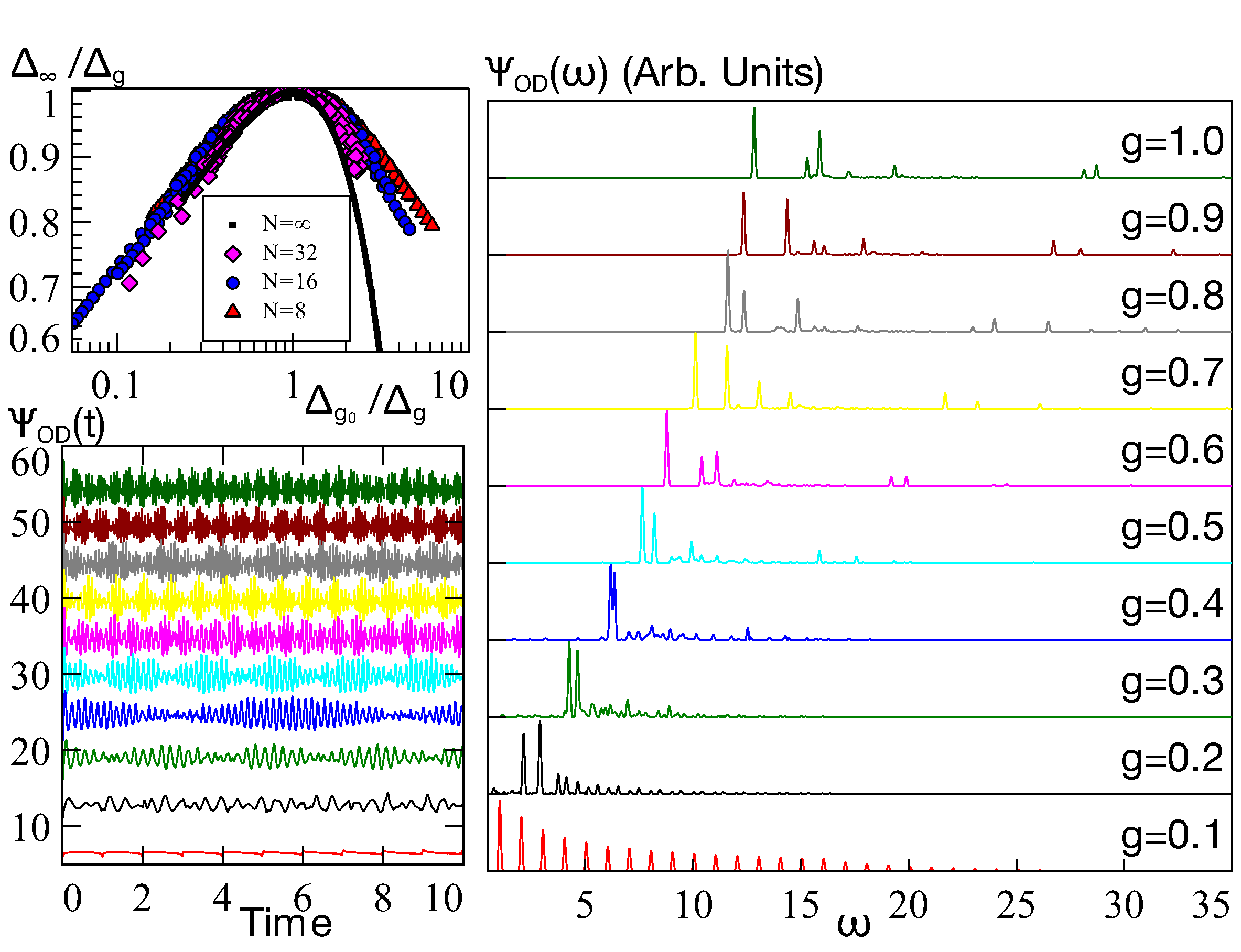
Figure 4: Bottom left: Off-diagonal order parameter evolution for $N=32$. Right: Fourier transform, the various plots are shifted on the vertical axis for clarity. Top Left: Non-equilibrium finite-size “phase diagram” resulting from the time-averaged canonical gap obtained from the off-diagonal order parameter, as explained in the text.

For small value of $g$, the various frequencies entering are very close to integers, as a result of the almost perfect equispacing of the levels. This regime could simply be described by perturbation theory and doesn’t show any striking features different from free fermions. With increasing $g$, the spectrum becomes very complicated since a large number of incommensurate frequencies contribute to the order parameter evolution. This is the realm of quantum fluctuations which makes the evolution highly irregular. Still increasing $g$, some regularity appears again. This can be understood in terms of results in the TD limit bl-06 . In fact, for $N\to\infty$, quenching from weak interaction to a much larger one, leads to an order parameter which shows persistent non-harmonic periodic evolution, i.e. a Fourier transform with equispaced peaks. Within the canonical description presented here, this feature will be reproduced when quenching to a large final value of $g$ since, as was shown in largeg , excited states in this regime form equispaced bands at energy $E\approx\Delta N_{G}+O(N^{0})$ ($N_{G}$ being the number of Gaudinos, i.e. the relevant excitations in this regime largeg ). As can be readily seen looking at the energy distribution of the points in Fig. 1, for finite large couplings, the low energy bands are already clearly formed, progressively collapsing into a single energy $E\approx\Delta N_{G}$. The slight remaining width of these bands would only result in additional low frequency corrections to the mean-field BCS result.

The static correlation functions studied in fcc-08 ; ao-02 depend mainly on low energy properties, and BCS-like behavior was always found when $g\gtrsim g^{*}=(2\ln N)^{-1}$, i.e. the criterion for the presence of superconductivity. In the problem at hand though, the quench matrix clearly shows that quantum quenches lead to an important occupation of the higher energy bands. These clearly differ from the BCS spectrum even for values of $g$ much larger than $g^{*}$ (that for $N=32$ is only $0.144\dots$). Quenches, since they probe high energy properties of the system, open up the possibility of probing interaction effects not captured by the mean-field treatment. Non mean-field features are manifest in non-equispaced dominant peaks in the frequency dependence of the order parameter. These accessible experimental quantities could thus be used as a spectroscopic tool (as proposed for other models in Ref. gdlp-07 ) to study quantum fluctuations.

We also considered the evolution of the canonical order parameter defined as $\Psi(t)=\sum_{\alpha=1}^{N}\sqrt{\frac{1}{4}-\left<S^{z}_{\alpha}(t)\right>^{2}}$, using the knowledge of the form factors for $S_{\alpha}^{z}$ (see Methods). It displays the same qualitative features as $\Psi_{OD}(t)$ and consequently will not be discussed here.

Let us conclude this section with a discussion of the long time asymptotic. It is difficult to extract any information about it from the highly irregular and oscillatory behavior reported in Fig. 4. Furthermore in finite system, (approximate) quantum recurrence will always spoil any signature of an eventual asymptotic state. However, if in the TD limit the asymptotic value of an observable exists, it must be equal to its time average, that is straightforwardly obtained with the tools at hand in finite systems. In fact, in Eq. (3) all the terms with $\nu\neq\xi$ average to zero and so $\overline{O}=\sum_{\nu}|Q^{0\nu}_{g_{0}g}|^{2}\langle\psi^{\nu}_{g}|O|\psi^{\nu}_{g}\rangle$, (the overline stands for the time average). $\overline{\Psi}_{OD}$ is obtained with little effort using the Hellmann-Feynman theorem $\langle\psi^{\nu}_{g}|\sum^{N}_{\alpha,\beta=1}S^{+}_{\alpha}S^{-}_{\beta}|\psi^{\nu}_{g}\rangle=-\frac{\partial\omega^{\nu}_{g}}{\partial g}$, thus without involving determinants. The non-equilibrium ‘phase diagram’ for $N\to\infty$ bl-06 shows that the final asymptotic value of the canonical gap $\Delta_{\infty}$ defines a universal curve when expressing $\Delta_{\infty}/\Delta_{g}$ vs $\Delta_{g_{0}}/\Delta_{g}$, where $\Delta_{g}$ is the equilibrium value at coupling $g$. In our normalization, $\Delta_{g}=g\Psi/N_{r}=g\sqrt{\Psi_{OD}/N_{r}-1}/N_{r}$ fcc-08 (the $-1$ cancels the first correction for large $N_{r}$). We take the last equation also off-equilibrium for the definition of the time averaged canonical gap in finite size. The resulting ‘finite-size phase diagram’ is reported in Fig. 4 (top left), where most of quenches from $g_{0}$ to $g$ both in $[0,1]$ are shown, for $N=8,16,32$ at half filling (we excluded the points with an equilibrium $\Psi_{OD}$ much different from BCS prediction, that are not expected to approach the asymptotic result). It is evident how increasing $N$ the curves tend to the Barankov-Levitov result shown as a full line .

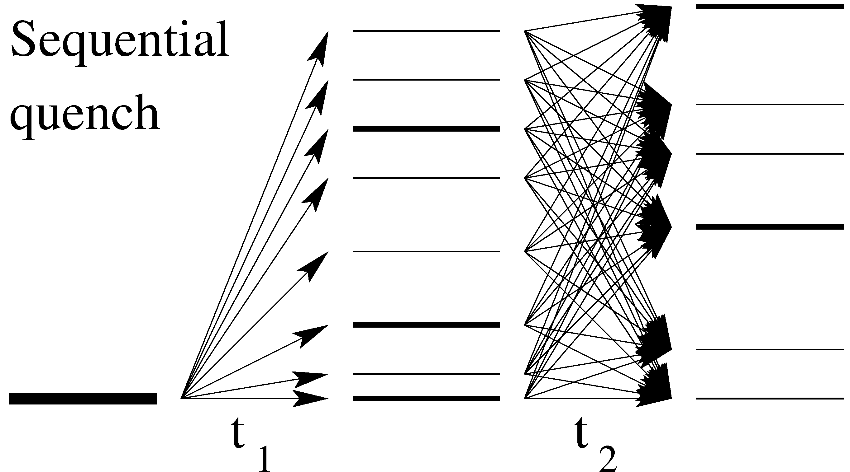
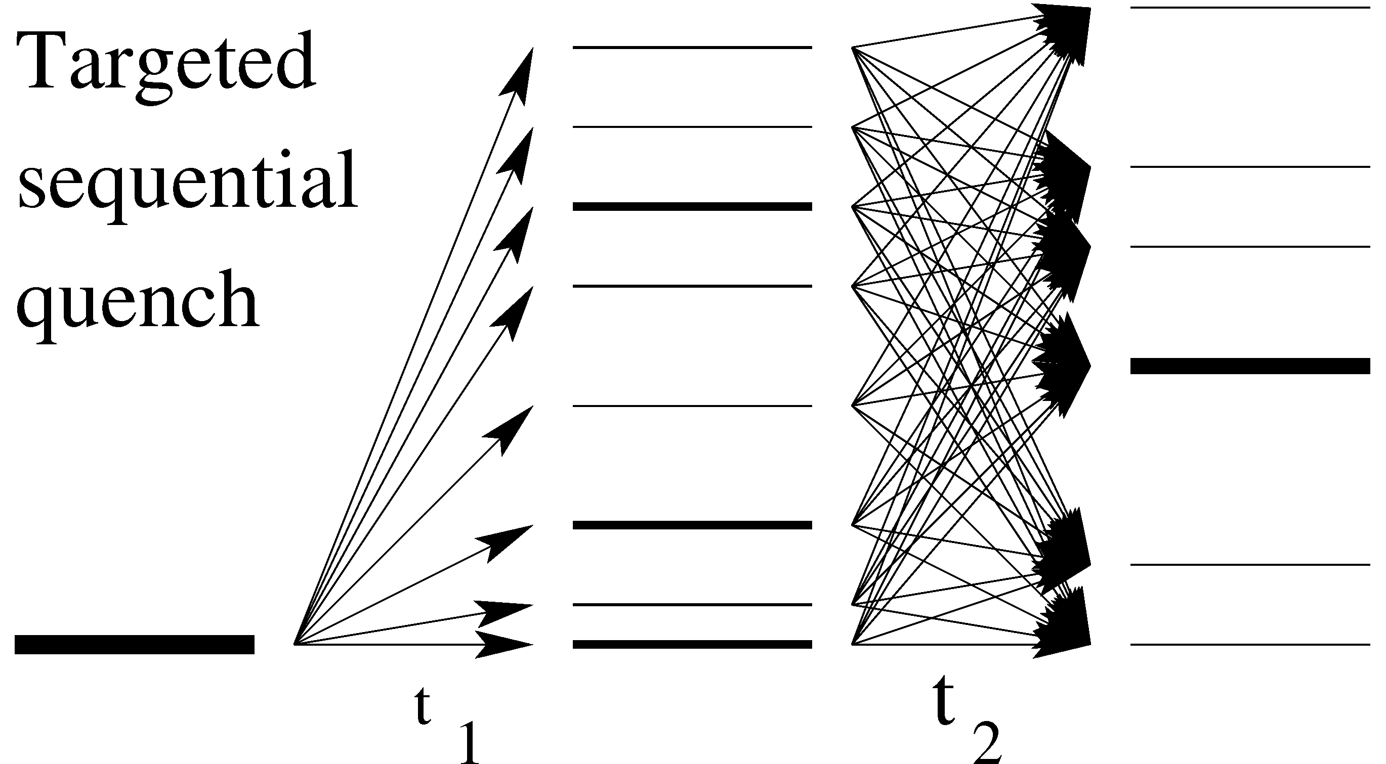
Figure 5: Left: A typical quench $g_{0}\to g$ populates all states according to the quench matrix. A general dequench $g\to g_{0}$ redistributes the weight among all states. Right: A targeted dequench after a chosen time can populate a targeted state.

THE DOUBLE QUENCH

We move now to address the very interesting dynamics that appear when we consider sequences of multiple quenches, $g_{i}\to g_{i+1}$ at times $t_{i}$. For brevity, we concentrate here on the problem of the double quench, or quench-dequench sequence, defined by $g=g_{0}$ for $t<0$, $g=g_{1}$ for $0\leq t<t_{q}$ and $g=g_{0}$ for $t\geq t_{q}$. Starting from a specific eigenstate of $H_{g_{0}}$, the quench at $t=0$ populates excited states of $H_{g_{1}}$ according to the quench matrix (2). Letting the system evolve up to time $t_{q}$ and then ‘dequenching’ back to $g_{0}$ results in a nontrivial amplitude of occupation for eigenstates of $H_{g_{0}}$, given by the quench propagator

$$P_{\beta\alpha}(t_{q})=\sum_{\gamma\in{\cal H}_{g_{1}}}Q_{g_{0}g_{1}}^{\beta\gamma}Q_{g_{1}g_{0}}^{\gamma\alpha}e^{-i\omega_{g_{1}}^{\gamma}t_{q}},$$ (10)

where $\alpha,\beta\in{\cal H}_{g_{0}}$ are respectively the labels for the pre- and post-quench states. For $t_{q}=0$, this propagator falls back onto the identity matrix. For finite duration $t_{q}>0$, interference effects lead to nontrivial states (see left panel of Fig. 5). For a specific initial state $\alpha$ and final state $\beta$, the quench propagator can be visualized as the sum of arrows of length $|Q_{g_{0}g_{1}}^{\beta\gamma}Q_{g_{1}g_{0}}^{\gamma\alpha}|$ rotating as a function of $t_{q}$ at frequency $\omega_{g_{1}}^{\gamma}$ from an initial phase $\mbox{arg}(Q_{g_{0}g_{1}}^{\beta\gamma}Q_{g_{1}g_{0}}^{\gamma\alpha})$. When arrows of non-negligible length align, constructive interference occurs, favoring the weight of the final state $\beta$ (see right panel of Fig. 5). Since all arrows rotate at different frequency, the occupation probability of state $\beta$ is a highly nontrivial function of the quench time, which is however completely characterized from the information we now have at hand.

We consider for definiteness a double quench starting from the ground state of Hamiltonian $H_{g_{0}}$. As a function of the quench duration $t_{q}$, the amplitudes of eigenstates $\alpha$ after the dequench will thus be given by $A_{\alpha}(t_{q})=P_{\alpha 0}(t_{q})$. We present in Fig. 6 the results of such double quench calculations. We specifically use a system of 16 spins, and trace over all intermediate states, allowing us to verify that the sum of square amplitudes remains equal to one (up to numerical accuracy of order $10^{-7}$) at all quench times. The top panel shows the ground state occupation, which is inevitably the dominant state for small $t_{q}$. However, we surprisingly find that its weight essentially vanishes (square amplitude below $0.005$), first around quench time $t_{q}=0.56$, and also repeatedly afterwards. The ground state is also periodically reconstructed to a large degree, showing that substantial sloshing of the occupation weight in the Hilbert space occurs as a function of the quench duration.

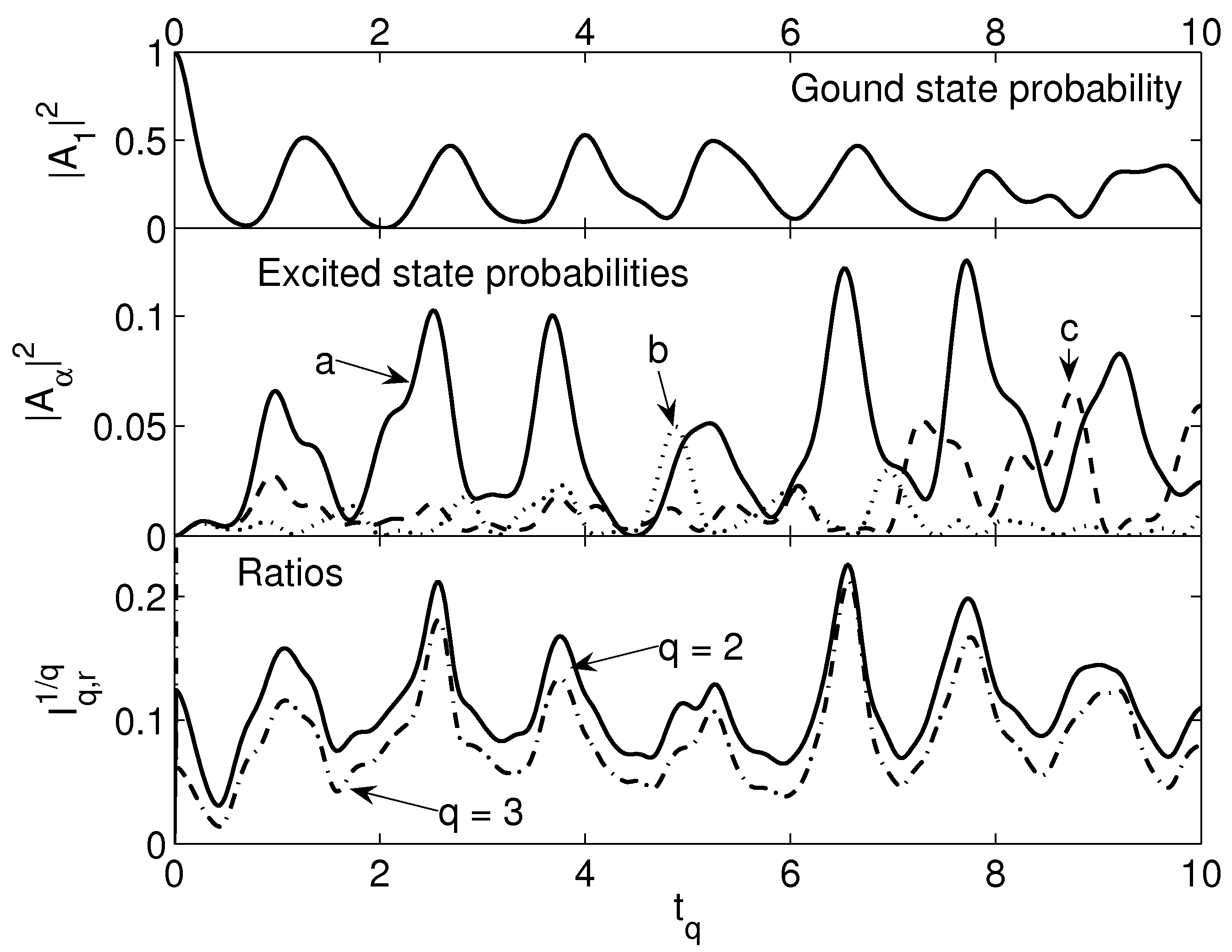
Figure 6: Occupation probabilities and moments after a double quench between $g=0$ and $0.5$, as a function of the quench duration $t_{q}$, for a system of 16 spins. The top plot gives the ground state occupation probability, clearly displaying vanishing and reconstruction effects. The middle plot gives the occupation probabilities for the three more relevant states. The lower graph shows the moments $I_{q}$, quantifying the degree of localization in Hilbert space after the double quench.

The occupation of individual excited states after the double quench also displays prominent time-dependent interference effects. Their amplitudes all begin at zero for $t_{q}=0$, but individual states can attain non-negligible amplitudes when the ‘arrows’ in their quench propagator add up constructively for particular quench durations. This is shown in the middle panel of Fig. 6, where we plot the occupation probability of three example states among the single block states. The times at which such alignments take place can be predicted using a simple algorithm based on what could be called a continuous sieve of Eratosthenes. Namely, for a given final state $\beta$, the double quench weights $|Q_{g_{0}g_{1}}^{\beta\gamma}Q_{g_{1}g_{0}}^{\gamma\alpha}|$ for all $\gamma$ are first ordered in decreasing value. The dominant mode (relabeled $0$) has a time-dependent phase $\phi^{0}(t_{q})=\omega_{g_{1}}^{0}t_{q}-\phi^{0}$ with $\phi^{0}\equiv{\rm arg}(Q_{g_{0}g_{1}}^{\beta\gamma^{0}}Q_{g_{1}g_{0}}^{\gamma^{0}\alpha})$, with similar defined phases for the subdominant modes $i>0$. Choosing an arbitrary phase alignment tolerance $\delta\theta$, the requirement that $|\phi^{i}(t_{q})-\phi^{0}(t_{q})|<\delta\theta$ for a given ‘arrow’ $i$ defines excluded time intervals on the quench timeline $t_{q}\in[0,\infty[$. Erasing all such intervals for all states up to a level $n$ leaves only the times at which all phases $\phi^{0}(t_{q}),...,\phi^{n}(t_{q})$ are aligned to the chosen tolerance, and for which a certain amount of constructive interference occurs. For example, in the middle panel of Fig. 6, the $b$ state peaks around $t_{q}\simeq 4.8$; it can be checked that this is a level $8$ alignment (with tolerance chosen as $\delta\theta=\pi/8$). Alignments of a given order $n$ and tolerance $\delta\theta$ occur more or less periodically. Increasing the order or reducing the tolerance $\delta\theta$ makes alignments of higher quality but quickly increasing rarity. In view of this sieve of Eratosthenes logic, an interesting question is whether the distribution of quench alignment times can be linked to that of e.g. prime numbers.

A study of the amplitudes $A_{\alpha}$ after a double quench for each individual final state is clearly prohibitive. Characterizing the distribution of amplitudes is more enlightening, and is best performed by exploiting tools common in the theory of localization in disordered systems, i.e. by considering the inverse participation ratios (IPRs) $I_{q}=\sum_{\alpha}|A_{\alpha}|^{2q}$, with $I_{1}=1$. In the bottom panel of Fig. 6, we plot the second and third IPRs for excited states (defined as $I_{q,r}=\sum_{\alpha>0}|A_{\alpha}|^{2q}/(\sum_{\alpha>0}|A_{\alpha}|^{2})^{q}$, i.e. summing over excited states only), which display the localization tendencies of the excited states’ amplitude weight in the Hilbert space after the double quench. Curves of $I_{2,r}$ and $I_{3,r}$ (always $\leq I_{2,r}$) approach one another when one excited state becomes dominant, and indicate smoother weight distribution otherwise.

Another interesting quantity to look at, which also has the advantage of being more directly accessible in experiments, is the work

$$W(t_{q})=\sum_{\alpha}(\omega_{g_{0}}^{\alpha}-\omega_{g_{0}}^{0})|A_{\alpha}(t_{q})|^{2}$$ (11)

or in other words the energy which is pumped into the system by a quench-dequench sequence of duration $t_{q}$. Starting from the ground state means that $W(t_{q})$ is strictly positive. Since the quench-dequench sequence populates excited states in a highly $t_{q}$ dependent way, this quantity will also display a rich frequency profile. In Fig. 7, we plot (inset) the work as a function of $t_{q}$, which displays nontrivial oscillatory behavior dominated by a frequency $\omega\simeq 4.62$ corresponding to the energy difference between the two dominant intermediate states during the quench. The Fourier transform $W(\omega_{q})$ is plotted in the main part of the figure, clearly displaying the above-mentioned peak but also the non-negligible contributions from a broad range of frequencies. The position of the peaks corresponds to excited energy level differences of the Hamiltonian during the quench, their height giving information on the size of the relevant quench matrix elements. The work can thus be used not only as a spectroscopic tool, but as a way to quantify eigenstate overlaps.

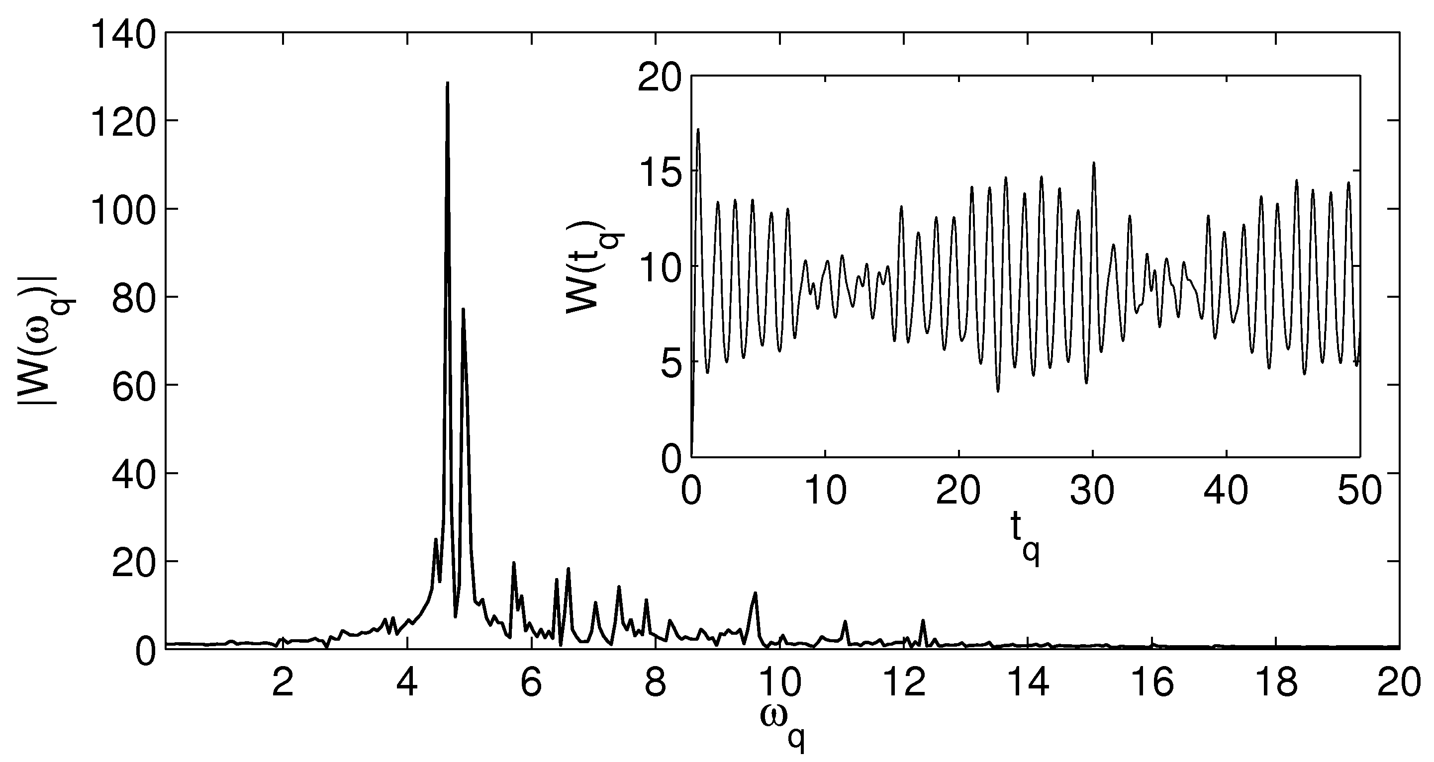
Figure 7: Total energy (work) pumped into the system by the quench-dequench sequence with $g_{0}=0$ and $g_{1}=0.5$ and $16$ spins, as a function of the quench duration $t_{q}$. Inset: work as a function of $t_{q}$ for the first oscillations of the envelope. These persist for much longer times, which are not plotted for clarity. Main plot: Fourier transform of the work, showing the main peak associated to the energy difference of the two dominant intermediate states.

DISCUSSIONS

In this work, we have proposed a novel method to tackle quantum quenches, based on integrability. We applied the method to the fermionic pairing model, showing the large amount of information that can be obtained on e.g. the work probability density, physical observables (and correlation functions) and their time evolution, and multiple quenches settings. Everything has been derived in an exact (or numerically exact) manner in the mesoscopic regime, where quantum fluctuations govern the dynamics. We gave evidence of how single and double quench dynamics can be effectively used to extract spectroscopic data from simple measurable quantities like the work done on the system.

To obtain these results we explored the peculiar property that the quench matrix of the pairing model can be obtained using Slavnov’s formula. This is not true in a general integrable model, and the generalization of the quench matrix representation is an open problem in the theory of integrable systems. When this representation will be available, the methods we propose here will allow exact calculations for a large variety of experimental relevant models, most importantly the one-dimensional Bose gas and Heisenberg spin chains.

Acknowledgments. We thank Boris L. Altshuler and Jan von Delft for useful discussions. This work was supported by the DFG through SFB631, SFB-TR12 and the Excellence Cluster ”Nanosystems Initiative Munich (NIM)”. All the authors are thankful for support from the Stichting voor Fundamenteel Onderzoek der Materie (FOM) in the Netherlands. PC benefited of a travel grant from ESF (INSTANS activity).

METHODS

Solving the Richardson equations

Because of the blocking effect excluding singly occupied levels from the dynamics rs-62 , Richardson’s model also has a pseudospin representation $S^{-}_{\alpha}=c_{\alpha\downarrow}c_{\alpha\uparrow}$, $S^{+}_{\alpha}=c^{\dagger}_{\alpha\uparrow}c^{\dagger}_{\alpha\downarrow}$, $S^{z}_{\alpha}=c^{\dagger}_{\alpha\uparrow}c^{\dagger}_{\alpha\downarrow}c_{\alpha\downarrow}c_{\alpha\uparrow}-1/2$. The Hamiltonian becomes

$$H=\sum^{N}_{\alpha=1}\epsilon_{\alpha}S^{z}_{\alpha}-g\sum^{N}_{\alpha,\beta=1}S^{+}_{\alpha}S^{-}_{\beta}\,$$ (12)

where $N$ is the number of unblocked levels.

At $g=0$ the $\binom{N}{N_{r}}$ solutions to the Richardson equations are trivial. They are given by Eq. (6) with the $N_{r}$ rapidities set to be strictly equal to one of the energies $\epsilon_{\alpha}$. Apart from a few particular cases with a small number of particles, the Richardson equations are not solvable analytically when $g\neq 0$, and one should solve them numerically. The solutions are such that every $w_{j}$ is either a real quantity or forms, with another parameter $w_{j^{\prime}}$, a complex conjugate pair (CCP), i.e. $w_{j^{\prime}}^{*}=w_{j}$. The mechanism for the CCPs formation is very easy: as interactions are turned on, all $w_{j}$ are real quantities for small enough $g$, but at a certain critical value of the coupling $g^{*}_{j}$ two rapidities will be exactly equal to one of the energy levels ($w_{j}=w_{j^{\prime}}=\epsilon_{\gamma}(j)$) and for $g>g^{*}_{j}$, the two parameters that collapsed will form a CCP at least for a finite interval in $g$. The situation is in fact rather intricate: the values $g^{*}_{j}$ are implicit functions of all other rapidities, and can only be read off a full solution of the Richardson equations for a specific choice of state. Moreover, CCPs can split back into real pairs, whose components can then re-pair with neighboring rapidities. Different choices of the parameters $\epsilon_{\alpha}$ and of their eventual degenerations specify different models. We specialize to the case of equally spaced levels. We make the choice to use $\epsilon_{\alpha}=\alpha$ which sets the zero of energy and implies that every energy will be given in units of the (pair) inter-level spacing. Furthermore we consider only half-filling of the energy levels $(N=2N_{r})$, when the number of rapidities $N_{r}$ equals the number of particles $N_{p}$, while in general in our notations $N_{r}+N_{p}=N$. At the precise value of $g$ at which a pair of rapidities $(w_{j},w_{j^{\prime}})$ collapse into a CCP $(w_{j}=w_{j^{\prime}}=\epsilon_{\gamma}(j))$, the Richardson equations (5) labelled $j$ and $j^{\prime}$ will include two diverging terms whose sum remains finite. In order to be able to treat these points numerically, one can define the real variables, $w_{1,j}\equiv w_{j}+w_{j^{\prime}}$ and $w_{2,j}\equiv(2\epsilon_{\gamma}(j)-w_{j}-w_{j^{\prime}})/(w_{j}-w_{j^{\prime}})^{2}$. As first discussed in r-66 , we need to know beforehand which rapidities will form a CCP and at which $\epsilon_{\gamma}(j)$ it will happen in order to use this type of change of variables. Here we find the various solutions to the Richardson equations numerically by increasing $g$ by small steps starting from the solution at $g=0$ and can therefore predict at every step, the upcoming formation of CCPs. As a consequence of this procedure, any given state at finite coupling can then be defined uniquely by the $g=0$ state from which it emerges (and the actual value of $g$).

Scalar products and Form factors

In Bethe Ansatz solvable models, Slavnov’s formula s-89 is an economical representation of the overlap of an eigenstate $|\{w\}\rangle$ with a general Bethe state $|\{v\}\rangle$ constructed using the same operators, but for which the set of rapidities $\{v\}$ does not fulfil the Bethe equations. This overlap is given as a determinant of an $N_{r}$ by $N_{r}$ matrix, which in the problem at hand reads zlmg-02 :

$$\langle\{w\}|\{v\}\rangle=\frac{{\rm det}_{N_{r}}J(\{v_{a}\},\{w_{b}\})\,\prod^{N_{r}}_{a\neq b}(v_{b}-w_{a})}{\prod_{b<a}(w_{b}-w_{a})\prod_{a<b}(v_{b}-v_{a})}\,,$$ (13)

with the matrix elements of $J$ given in Ref. zlmg-02 ; fcc-08 ,

$$J_{ab} = \frac{v_{b}-w_{b}}{v_{a}-w_{b}}\left[\sum^{N}_{\alpha=1}\frac{1}{(v_{a}-\epsilon_{\alpha})(w_{b}-\epsilon_{\alpha})}\right.$$ (14)

$$\left.-2\sum_{c\neq a}^{N_{r}}\frac{1}{(v_{a}-v_{c})(w_{b}-v_{c})}\right].$$

The solution to the inverse problem allows a determinant representation for the necessary form factors zlmg-02

$$\langle\{w\}|S^{z}_{\alpha}|\{v\}\rangle=\prod^{N_{r}}_{a=1}\frac{(w_{a}-\epsilon_{\alpha})}{(v_{a}-\epsilon_{\alpha})}\frac{{\rm det}_{N_{r}}\left(\frac{1}{2}{\cal T}-{\cal Q}(\alpha)\right)}{\displaystyle\prod_{b>a}(w_{b}-w_{a})\prod_{b<a}(v_{b}-v_{a})}\,,$$

with the matrix elements of ${\cal T},{\cal Q}$ given by

$${\cal T}_{ab}=\frac{2\displaystyle\prod^{N_{r}}_{{c\neq a}}(w_{c}-v_{b})}{w_{a}-v_{b}}\left[\sum_{c\neq b}\frac{1}{(v_{b}-v_{c})}-\sum_{c\neq a}\frac{1}{(v_{b}-w_{c})}\right],$$

$${\cal Q}_{ab}(\alpha)=\frac{\prod_{c\neq b}(v_{c}-v_{b})}{(w_{a}-\epsilon_{\alpha})^{2}}.$$ (15)

We explicitly used the fact that both states are solutions to the Richardson equations in order to write the matrix elements of ${\cal T}$ in a more compact form than in previous publications zlmg-02 ; fcc-08 .

The form factors for $S^{-}_{\alpha}S^{+}_{\beta}$ can be written as sum of $N_{r}$ determinants by generalizing the method of Ref. fcc-08 for $\{v\}=\{w\}$ starting from the double sums in Ref. zlmg-02 . For $\alpha\neq\beta$ we have

$$\langle\{v\}|S^{-}_{\alpha}S^{+}_{\beta}|\{w\}\rangle = \frac{\displaystyle\prod_{c}\left(\frac{v_{c}-\epsilon_{\alpha}}{w_{c}-\epsilon_{\alpha}}\right)\displaystyle\prod_{k\neq q}\left(w_{k}-w_{q}\right)}{\displaystyle\prod_{b>a}(v_{a}-v_{b})\prod_{a>b}(w_{a}-w_{b})}$$ (16)

$$\times \sum_{q=1}^{N_{r}}\frac{w_{q}-\epsilon_{\alpha}}{w_{q}-\epsilon_{\beta}}{\rm det}{\cal J}^{q}_{\alpha,\beta}\,,$$

where, defining $A_{ab}=J_{ab}\displaystyle\prod_{c\neq b}(v_{c}-w_{b})$, the matrix elements are given by

$${\cal J}_{ab} = A_{ab}-\frac{\prod_{k\neq b,q}(w_{k}-w_{b})}{\prod_{k\neq b+1,q}(w_{k}-w_{b+1})}$$

$$\times\frac{w_{b}-\epsilon_{\alpha}}{w_{b+1}-\epsilon_{\alpha}}A_{ab+1},\ \ b<q-1,$$

$${\cal J}_{aq-1} = A_{aq-1}+2\frac{(w_{q}-\epsilon_{\beta})(w_{q-1}-\epsilon_{\alpha})}{w_{q-1}-w_{q}}\prod_{c}\left(\frac{v_{c}-\epsilon_{\beta}}{w_{c}-\epsilon_{\beta}}\right)$$

$$\times\prod_{k\neq q-1}(w_{k}-w_{q-1})\frac{(2v_{a}-\epsilon_{\alpha}-\epsilon_{\beta})}{(v_{a}-\epsilon_{\alpha})^{2}(v_{a}-\epsilon_{\beta})^{2}},$$

$${\cal J}_{aq} = 1/(v_{a}-\epsilon_{\alpha})^{2},$$

$${\cal J}_{ab} = A_{ab},\ \ \ b>q\,.$$ (17)

For $\alpha=\beta$ they are calculated using Hellmann-Feynman theorem as explained in the main text.

References

-
(1)
M. Greiner, O. Mandel, T. W. Hänsch, & I. Bloch,
Collapse and revival of the matter wave field of a Bose-Einstein condensate,
Nature 419, 51 (2002);
T. Kinoshita , T. Wenger, & D. S. Weiss, A quantum Newton’s cradle, Nature 440, 900 (2006);
L.E. Sadler, J. M. Higbie, S. R. Leslie, M. Vengalattore, & D. M. Stamper-Kurn, Spontaneous symmetry breaking in a quenched ferromagnetic spinor Bose-Einstein condensate, Nature 443, 312 (2006);
S. Hofferberth, I. Lesanovsky, B. Fischer, T. Schumm, & J. Schmiedmayer, Non-equilibrium coherence dynamics in one-dimensional Bose gases, Nature 449, 324 (2007);
C. N. Weiler, T. W. Neely, D. R. Scherer, A. S. Bradley, M. J. Davis & B. P. Anderson, Spontaneous vortices in the formation of Bose-Einstein condensates, Nature 455, 948 (2008). -
(2)
M. Cramer, C.M. Dawson, J. Eisert, & T.J. Osborne,
Quenching, relaxation, and a central limit theorem for quantum lattice systems,
Phys. Rev. Lett. 100, 030602 (2008);
C. Kollath, A. Laeuchli, & E. Altman, Quench dynamics and non equilibrium phase diagram of the Bose-Hubbard model, Phys. Rev. Lett. 98, 180601 (2007);
S. R. Manmana, S. Wessel, R. M. Noack, & A. Muramatsu, Strongly correlated fermions after a quantum quench, Phys. Rev. Lett. 98, 210405 (2007);
M. Rigol, V. Dunjko, V. Yurovsky, & M. Olshanii, Relaxation in a completely integrable many-body quantum system: An ab initio study of the dynamics of the highly excited states of lattice hard-core bosons, Phys. Rev. Lett. 98, 050405 (2007);
T. Barthel T & U. Schollwock, Dephasing and the steady state in quantum many-particle systems Phys. Rev. Lett. 100, 100601 (2008);
M. Cramer, A. Flesch, I. P. McCulloch, U. Schollwoeck, & J. Eisert, Exploring local quantum many-body relaxation by atoms in optical superlattices, Phys. Rev. Lett. 101, 063001 (2008);
M. Rigol, V. Dunjko, & M. Olshanii, Thermalization and its mechanism for generic isolated quantum systems, Nature 452, 854 (2008);
A. Laeuchli & C. Kollath, Spreading of correlations and entanglement after a quench in the one-dimensional Bose-Hubbard model, J. Stat. Mech. (2008) P05018;
P. Barmettler, A. M. Rey, E. Demler, M. D. Lukin, I. Bloch, & V. Gritsev, Quantum many-body dynamics of coupled double-well superlattices, Phys. Rev. A 78, 012330 (2008);
A. Flesch, M. Cramer, I.P. McCulloch, U. Schollwoeck, & J. Eisert, Probing local relaxation of cold atoms in optical superlattices, Phys. Rev. A 78, 033608 (2008);
G. Roux, On quenches in non-integrable quantum many-body systems: the one-dimensional Bose-Hubbard model revisited, 0810.3720;
P. Barmettler, M. Punk, V. Gritsev, E. Demler & E. Altman, Relaxation of antiferromagnetic order in spin-1/2 chains following a quantum quench, 0810.4845;
S. R. Manmana, S. Wessel, R. M. Noack, & A. Muramatsu, Time evolution of correlations in strongly interacting fermions after a quantum quench, 0812.0561. -
(3)
P. Calabrese & J. Cardy,
Time-dependence of correlation functions following a quantum quench,
Phys. Rev. Lett. 96, 136801 (2006);
P. Calabrese & J. Cardy, Quantum quenches in extended systems, J. Stat. Mech. P06008 (2007). - (4) V. Gritsev, E. Demler, M. Lukin, & A. Polkovnikov, Spectroscopy of collective excitations in interacting low-dimensional many-body systems using quench dynamics, Phys. Rev. Lett. 99, 200404 (2007).
-
(5)
E. Barouch, B. McCoy, & M. Dresden,
Statistical mechanics of the XY model. I,
Phys. Rev. A 2, 1075 (1970);
E. Barouch & B. McCoy, Statistical mechanics of the XY model. III, Phys. Rev. A 3, 3127 (1971);
F. Igloi & H. Rieger, Long-Range correlations in the nonequilibrium quantum relaxation of a spin chain, Phys. Rev. Lett. 85, 3233 (2000);
K. Sengupta, S. Powell, & S. Sachdev, Quench dynamics across quantum critical points, Phys. Rev. A 69, 053616 (2004);
P. Calabrese & J. Cardy, Evolution of entanglement entropy in one dimensional systems, J. Stat. Mech. P04010 (2005);
R. W. Cherng & L. S. Levitov, Entropy and correlation functions of a driven quantum spin chain, Phys. Rev. A 73, 043614 (2006);
V. Mukherjee, U. Divakaran, A. Dutta, & D. Sen, Quenching dynamics of a quantum XY spin-1/2 chain in a transverse field, Phys. Rev. B 76, 174303 (2007);
V. Eisler & I. Peschel, Entanglement in a periodic quench, Ann. Phys. (Berlin) 17, 410 (2008);
M. Fagotti & P. Calabrese, Evolution of entanglement entropy following a quantum quench: Analytic results for the XY chain in a transverse magnetic field, Phys. Rev. A 78, 010306(R) (2008);
V. Mukherjee, A. Dutta, & D. Sen, Defect generation in a spin-1/2 transverse XY chain under repeated quenching of the transverse field, Phys. Rev. B 77, 214427 (2008);
D. Rossini, A. Silva, G. Mussardo & G. Santoro, Effective thermal dynamics following a quantum quench in a spin chain, 0810.5508. - (6) A. Silva, The statistics of the work done on a quantum critical system by quenching a control parameter, Phys. Rev. Lett. 101, 120603 (2008).
- (7) H. Bethe, Zur theorie der metalle, Z. Phys. 71, 205 (1931).
- (8) V. E. Korepin, N. M. Bogoliubov & A. G. Izergin A G, Quantum Inverse Scattering Method and Correlation Functions, Cambridge University Press (1993).
- (9) M. Takahashi, Thermodynamics of one-dimensional solvable models, Cambridge University Press (1999).
- (10) N. A. Slavnov, On scalar products in the algebraic Bethe ansatz, Teor. Mat. Fiz. 79, 232 (1989).
- (11) N. Kitanine, J. M. Maillet, & V. Terras, Correlation functions of the XXZ Heisenberg spin-1/2 chain in a magnetic field, Nucl. Phys. B 554, 647 (1999).
-
(12)
J.-S. Caux & J.-M. Maillet,
Computation of dynamical correlation functions of Heisenberg chains in a field,
Phys. Rev. Lett. 95, 077201 (2005);
J.-S. Caux, R. Hagemans & J.-M. Maillet, Computation of dynamical correlation functions of Heisenberg chains: the gapless anisotropic regime, J. Stat. Mech. P09003 (2005). -
(13)
J.-S. Caux & P. Calabrese,
Dynamical density-density correlations in the one-dimensional Bose gas,
Phys. Rev. A 74, 031605 (2006);
J.-S. Caux, P. Calabrese & N. A. Slavnov, One-particle dynamical correlations in the one-dimensional Bose gas, J. Stat. Mech. P01008 (2007). -
(14)
R. W. Richardson,
A restricted class of exact eigenstates of the pairing-force Hamiltonian,
Phys. Lett. 3, 277 (1963);
R. W. Richardson, Application to the exact theory of the pairing model to some even isotopes of lead, Phys. Lett. 5, 82 (1963);
R. W. Richardson & N. Sherman, Exact eigenstates of the pairing-force Hamiltonian, Nucl. Phys. 52, 221 (1964);
R. W. Richardson & N. Sherman, Pairing models of Pb206, Pb204 and Pb202, Nucl. Phys. 52, 253 (1964). -
(15)
J. von Delft & D. C. Ralph, Spectroscopy of discrete energy levels in
ultrasmall metallic grains,
Phys. Rep. 345, 61 (2001);
J. Dukelsky S. Pittel & G. Sierra, Exactly solvable Richardson-Gaudin models for many-body quantum systems, Rev. Mod. Phys. 76, 643 (2004). -
(16)
J. Bardeen, L. N. Cooper & J. R. Schrieffer,
Microscopic theory of superconductivity,
Phys. Rev. 106, 162 (1957);
J. Bardeen, L. N. Cooper & J. R. Schrieffer, Theory of superconductivity, Phys. Rev. 108, 1175 (1957). -
(17)
H.-Q. Zhou J. Links, R.H. McKenzie, & M.D. Gould,
Superconducting correlations in metallic nanoparticles: exact solution of the
BCS model by the algebraic Bethe ansatz,
Phys. Rev. B 65, 060502(R) (2002);
J. Links, H.-Q. Zhou, R.H. McKenzie, & M.D. Gould, Algebraic Bethe ansatz method for the exact calculation of energy spectra and form factors: applications to models of Bose-Einstein condensates and metallic nanograins, J. Phys. A 36, R63 (2003). - (18) A. Faribault, P. Calabrese, & J.-S. Caux, Exact mesoscopic correlation functions of the pairing model, Phys. Rev. B 77, 064503 (2008).
- (19) R. A. Barankov & L. S. Levitov, Synchronization in the BCS pairing dynamics as a critical phenomenon, Phys. Rev. Lett. 96, 230403 (2006).
-
(20)
E. A. Yuzbashyan, B. L. Altshuler, V. B. Kuznetsov, & V. Z. Enolskii,
Nonequilibrium Cooper pairing in the nonadiabatic regime,
Phys. Rev. B 72, 220503(R) (2005);
E. A. Yuzbashyan & M. Dzero, Dynamical vanishing of the order parameter in a fermionic condensate, Phys. Rev. Lett. 96, 230404 (2006);
E. A. Yuzbashyan, O. Tsyplyatyev, & B. L. Altshuler, Relaxation and persistent oscillations of the order parameter in the non-stationary BCS theory, Phys. Rev. Lett. 96, 097005 (2006);
M. Dzero, E. A. Yuzbashyan, B. L. Altshuler, & P. Coleman, Spectroscopic signatures of nonequilibrium pairing in atomic Fermi gases, Phys. Rev. Lett. 99, 160402 (2007);
R. A. Barankov & L. S. Levitov, Excitation of the dissipationless Higgs mode in a fermionic condensate, 0704.1292;
A. Tomadin, M. Polini, M. P. Tosi, & R. Fazio, Nonequilibrium pairing instability in ultracold Fermi gases with population imbalance, Phys. Rev. A 77, 033605 (2008). -
(21)
J. M. Roman, G. Sierra, & J. Dukelsky,
Elementary excitations of the BCS model in the canonical ensemble,
Phys. Rev. B 67, 064510 (2003);
E. A. Yuzbashyan, A. A. Baytin, & B. L. Altshuler, Strong coupling expansion for the pairing Hamiltonian, Phys. Rev. B 68, 214509 (2003). -
(22)
A. Mastellone, G. Falci, & R. Fazio,
A small superconducting grain in the canonical ensemble,
Phys. Rev. Lett. 80, 4542 (1998);
L. Amico & A. Osterloh, Exact correlation functions of the BCS model in the canonical ensemble, Phys. Rev. Lett. 88, 127003 (2002). - (23) R. W. Richardson, Numerical study of the 8-32-particle eigenstates of the pairing Hamiltonian, Phys. Rev. 141, 949 (1966).