Phase Diagram of spin 1/2 XXZ Model With Dzyaloshinskii-Moriya Interaction

Abstract

We have studied the phase diagram of the one dimensional XXZ model with Dzyaloshinskii-Moriya (DM) interaction. We have applied the quantum renormalization group (QRG) approach to get the stable fixed points, critical point and the scaling of coupling constants. This model has three phases, ferromagnetic, spin-fluid and Néel phases which are separated by a critical line which depends on the DM coupling constant. We have shown that the staggered magnetization is the order parameter of the system and investigated the influence of DM interaction on the chiral ordering as a helical magnetic order.

I Introduction

Quantum phase transition has been one of the most interesting topic in the area of strongly correlated systems in the last decade. It is a phase transition at zero temperature where the quantum fluctuations play the dominant role vojta . Suppression of the thermal fluctuations at zero temperature introduces the ground state as the representative of the system. The properties of the ground state may be changed drastically shown as a non-analytic behavior of a physical quantity by reaching the quantum critical point (QCP). This can be done by tuning a parameter in the Hamiltonian, for instance the magnetic field or the amount of disorder. The ground state of a typical quantum many body systems consist of a superposition of a huge number of product states. Understanding this structure is equivalent to establishing how subsystems are interrelated, which in turn is what determines many of the relevant properties of the system. In Mott insulators the Heisenberg interaction is in most cases the dominant source of coupling between local moments, and most theoretical investigations are based on modeling in which only this type of interaction is included. Recently some novel magnetic properties in antiferromagnetic (AF) systems were discovered in the variety of quasi-one dimensional materials that are known to belong to an antisymmetric interaction of the form $\overrightarrow{D}.(\overrightarrow{S_{i}}\times\overrightarrow{S_{j}})$ which is known as the Dzyaloshinskii-Moriya (DM)interaction. The relevance of antisymmetric superexchange interactions in spin Hamiltonian which leads to either a week ferromagnetic (F) or helical magnetic distortion in quantum AF systems, has been introduced phenomenologically by DzyaloshinskiiDzyaloshinskii . A microscopic model of antisymmetric exchange interaction was first proposed by MoriyaMoriya which showed that such interactions arise naturally in perturbation theory due to the spin-orbit coupling in magnetic systems with low symmetry and is essentially an extension of the Anderson superexchange mechanismAnderson that shows for spin-flip hopping of electrons. Since it (DM interaction) breaks the fundamental SU(2) symmetry of the Heisenberg interactions, it is at the origin of many deviations from pure heisenberg behavior such as cantingCoffey or small gapsDender1 ; Oshikawa1 ; Zhao ; Fouet ; Chernyshev . A number of AF systems expected to be described by DM interaction, such as $Cu(C_{6}D_{5}COO)_{2}3D_{2}O$Dender1 ; Dender2 , $Yb_{4}As_{3}$Kohgi ; Fulde ; Oshikawa2 , $BaCu_{2}Si_{2}O_{7}$Tsukada , $\alpha-Fe_{2}O_{3}$, $LaMnO_{3}$Grande and $K_{2}V_{3}O_{8}$Greven , which exhibit unusual and interesting magnetic properties in the presence of quantum fluctuations and/or applied magnetic fieldGrande ; Yildirim ; Katsumata . Also belonging to the class of DM antiferromagnets is $La_{2}CuO_{4}$, which is a parent compound of high-temperature superconductorsKastner . This has stimulated extensive investigation on the physical properties of the DM interaction. However, This interaction is rather difficult to Handel analytically, which has brought much uncertainty in the interpretation of experimental data and has limited our understanding of many interesting quantum phenomena of low-dimensional magnetic materials.

In the present paper, we have considered the one dimensional XXZ model with DM interaction by implementing the quantum renormalization group (QRG) method. In the next section the QRG approach will be explained and the renormalization of coupling constant are obtained. In section (III), we will obtain the phase diagram, fixed points, critical points and calculate the staggered magnetization as the order parameter of the underling quantum phase transition. We will also introduce the chiral order as an ordering which is produced by DM interaction. The exponent which shows the divergence of correlation function close to the critical point $(\nu)$, the dynamical exponent $(z)$ and the exponent which shows the vanishing of staggered magnetization near the critical point $(\beta)$ will also be calculated. In Sec (IV), discussion concludes the paper.

II Quantum renormalization group

The main idea of the RG method is the elimination or the thinning of the degrees of freedom caried out step by step in an iteration procedure. Here, we used the well known Kadanoff block method as it is both well suited to perform analytical calculations in the lattice models and is conceptually straight-forward to be extended to the higher dimensionsmiguel1 ; miguel-book ; Langari ; Jafari . In the Kadanoff’s method, the lattice is divided into blocks in which the Hamiltonian can be exactly diagonalized. Selecting a number of low-lying eigenstates of the blocks the full Hamiltonian is projected onto these eigenstates and an the effective (renormalized) Hamiltonian is obtained.

The Hamiltonian of XXZ model with DM interaction in the $z$ direction on a periodic chain of $N$ sites is

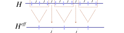
Figure 1: (color online)The decomposition of chain into three site blocks Hamiltonian ($H^{B}$) and inter-block Hamiltonian ($H^{BB}$).

$$H(J,\Delta)=\frac{J}{4}\sum_{i}^{N}\Big{[}\sigma_{i}^{x}\sigma_{i+1}^{x}+\sigma_{i}^{y}\sigma_{i+1}^{y}+\Delta\sigma_{i}^{z}\sigma_{i+1}^{z}$$ (1)

$$+D(\sigma_{i}^{x}\sigma_{i+1}^{y}-\sigma_{i}^{y}\sigma_{i+1}^{x})\Big{]},$$

where the $J$ is exchange constant, $D$ is the strength of $z$ component of DM interaction and the easy-axis anisotropy defined by $\Delta$ which can be positive and negative. The positive and negative $J$ corresponds to the antiferromagnetic and ferromagnetic (F) cases, respectively. $\sigma_{i}^{\alpha}$ refers to the $\alpha$-component of the Pauli matrix at site $i$. By implement $\pi$ rotation around $z$ axis on odd or even sites, the AF case of Hamiltonian ($J>0$) is mapped on the F case ($J<0$) with opposite sign of anisotropy,

$$H(J,\Delta)=\frac{J}{4}\sum_{i}^{N}\Big{[}\sigma_{i}^{x}\sigma_{i+1}^{x}+\sigma_{i}^{y}\sigma_{i+1}^{y}-\Delta\sigma_{i}^{z}\sigma_{i+1}^{z}$$ (2)

$$+D(\sigma_{i}^{x}\sigma_{i+1}^{y}-\sigma_{i}^{y}\sigma_{i+1}^{x})\Big{]},~{}~{}J>0.$$

So we can restrict ourselves to AF case ($J>0$) with $D>0$ and arbitrary anisotropy ($\Delta<0$ and $\Delta>0$) without loss of generality.

The effective Hamiltonian to the first order RG approximation is

$$H^{eff}=H^{eff}_{0}+H^{eff}_{1},~{}~{}~{}~{}~{}~{}~{}~{}~{}$$

$$H^{eff}_{0}=P_{0}H^{B}P_{0}~{}~{}~{},~{}~{}~{}H^{eff}_{1}=P_{0}H^{BB}P_{0}.$$

We consider a three-site block procedure defined in Fig.(1). The block Hamiltonian $(H_{B}=\sum h_{I}^{B})$, its eigenstates and eigenvalues are given in Appendix A. The three-site block Hamiltonian has four doubly degenerate eigenvalues (see Appendix A). $P_{0}$ is the projection operator of the ground state subspace defined by $\big{(}P_{0}=|\Uparrow\rangle\langle\psi_{0}|+|\Downarrow\rangle\langle\psi_{0}^{\prime}|\big{)}$, Where $|\psi_{0}\rangle$ and $|\psi_{0}^{\prime}\rangle$ are the doubly degenerate ground states, $|\Uparrow\rangle$ and $|\Downarrow\rangle$ are the renamed base kets in the effective Hilbert space. For each block we keep two states ($|\psi_{0}\rangle$ and $|\psi_{0}^{\prime}\rangle$) to define the effective (new) site. Thus, the effective site can be considered as having a spin 1/2. Due to the level crossing which occurs for the eigenstates of the block Hamiltonian, the projection operator ($P_{0}$) can be different depending on the coupling constants. Therefore, we must specify different regions with the corresponding ground states. As Fig.(5) shows there are two regions with different eigenstates which are separated by $\Delta<-\sqrt{1+D^{2}}$ where a level crossing occurs. In region (A) the ground state is the doubly-degenerate ferromagnetic state $|\psi_{3}\rangle$ and $|\psi_{3}^{\prime}\rangle$ while in region (B) $|\psi_{0}\rangle$ and $|\psi_{0}^{\prime}\rangle$ are the degenerate ground states. At the level crossing ($\Delta=-\sqrt{1+D^{2}}$) the ground state is 4-fold degenerate ($|\psi_{3}\rangle$, $|\psi_{3}^{\prime}\rangle$, $|\psi_{0}\rangle$, $|\psi_{0}^{\prime}\rangle$). A summary of this information is given in Fig.(5) of appendix A.

In the following, we will classify the RG equation of the regions where each of this states represent the ground state.

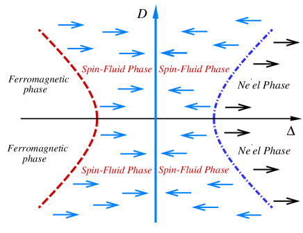
Figure 2: (color online) Phase diagram of the XXZ model with DM interaction. The long dashed line is the critical line which separates SF-Néel phases and is characterized by $\Delta_{c}=(1+D^{2})^{1/2}$. The dashed dot line shows the level crossing which separate SF-F phases is given by $\Delta=-(1+D^{2})^{1/2}$ . Arrows show the running of coupling constant under RG iteration.

II.1 Region (A): $e_{0}$ is the ground state.

In this region the effective Hamiltonian in the first order correction is similar to the initial one, i.e,

$$H^{eff}=\frac{J^{\prime}}{4}\sum_{i}^{N}\Big{[}\sigma_{i}^{x}\sigma_{i+1}^{x}+\sigma_{i}^{y}\sigma_{i+1}^{y}+{\Delta^{\prime}}\sigma_{i}^{z}\sigma_{i+1}^{z}$$

$$+D^{\prime}(\sigma_{i}^{x}\sigma_{i+1}^{y}-\sigma_{i}^{y}\sigma_{i+1}^{x})\Big{]}$$ (3)

where $J^{\prime}$, $\Delta^{\prime}$ and $D^{\prime}$ are the renormalized coupling constants. The new renormalized coupling constants are found to be functions of the original ones given by the following equations,

$$J^{\prime}=J(\frac{2}{q})^{2}(1+D^{2}),~{}~{}D^{\prime}=D$$ (4)

$$\Delta^{\prime}=\frac{\Delta}{1+D^{2}}(\frac{\Delta+q}{4})^{2}.$$

II.2 Region (B): $e_{3}$ is the ground state.

In this region the effective Hamiltonian to the first order corrections leads to the ferromagnetic Ising model

$$H^{eff}=\frac{1}{4}\left[\Delta^{\prime}\sum_{i}^{N/3}{\sigma}_{i}^{z}{\sigma}_{i+1}^{z}\right],$$

where

$$\Delta^{\prime} = J\Delta,~{}~{}J>0,~{}~{}\Delta<0.$$

III Phase Diagram

III.1 Region (A)

For simplicity we have separated this region into positive anisotropy and negative anisotropy sectors.

• $\Delta>0$

  In the positive anisotropy sector the RG equations show that the $J$ coupling, representing the energy scale, approaching zero by iterating RG procedure. Thus, at the zero temperature,the quantum phase transition is the result of competition between the anisotropy ($\Delta$) and the DM coupling constant ($D$). In the region of planar anisotropy $0<\Delta<1$, the symmetric interactions ($D=0$) is known not to support any kind of long range order and the ground state is the so called spin-fluid (SF) state. Increasing the amount of anisotropy is necessary to stabilize the spin alignment. For $\Delta>1$ the ground state is the Néel ordered state. In the case of $D\neq 0$, the anisotropy constant ($\Delta$) and antisymmetric (DM) coupling are in competition with each other. The latter thus destroys the ordering tendency of the former and defers creating of Néel order. Our RG equations show that the phase boundary between the SF and Néel phases which depends on the DM coupling is $\Delta_{c}=\sqrt{1+D^{2}}$ (see Fig.(2)) which agrees with the phase boundary reported in Ref.Alcaraz, . This critical line coincide with boundary line which obtained by classical approximation (see appendix C). The RG equations (Eq.(4)) express the DM coupling dose not flow under RG transformations, and the anisotropy coupling goes to zero ($\Delta\rightarrow 0$) in SF phase while it scales to infinity ($\Delta\rightarrow\infty$) in the Néel phase.

  We have linearized the RG flow at the critical line $\Delta_{c}=\sqrt{1+D^{2}}$ and found one relevant and one marginal directions. The eigenvalues of the matrix of linearized flow are $\lambda_{1}=\frac{5}{3}$, $\lambda_{2}=1$. The corresponding eigenvectors in the $|\Delta,D\rangle$ coordinates are $|\lambda_{1}\rangle=|1,0\rangle$, $|\lambda_{2}\rangle=|\frac{D}{\sqrt{1+D^{2}}},1\rangle$. The marginal direction corresponds to the tangent line of the critical line and the relevant direction shows the direction of anisotropy’s flow (Fig.(2)).

  

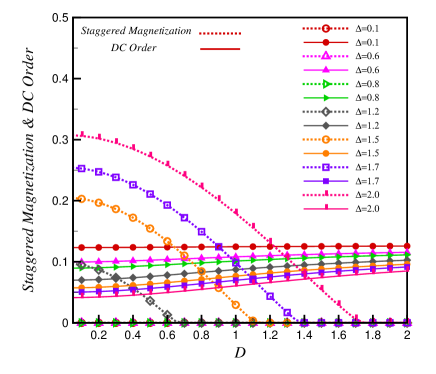
  Figure 3: (color online) DC order (solid lines) and Staggered Magnetization (dotted lines) versus D.

  

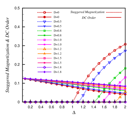
  Figure 4: (color online) DC order (solid lines) and Staggered Magnetization (dotted lines) versus $\Delta$.

  However we have found the boundary of the SF-Néel transition by calculating the staggered magnetization $S_{M}$ (see appendix B) in the $z$-direction as an order parameter (Fig.(3) and Fig.(4)),

  $$S_{M}=\frac{1}{N}\sum_{i=1}^{N}(\frac{(-1)^{i}}{2})\langle\sigma_{i}^{z}\rangle.$$ (5)

  $S_{M}$ is zero in the SF phase and has a nonzero value in the Néel phase. Thus the staggered magnetization is the proper order parameter to represent the SF-Néel transition. We have plotted $S_{M}$ versus $D$ and versus $\Delta$ in Fig.(3) and Fig.(4), respectively. In Fig.(3) it is obvious that the staggered magnetization goes to zero continuously at the critical value of $D_{c}$ which shows the destruction of Néel order. The critical value $D_{c}$ where the staggered magnetization vanishes above it, increases by increasing of anisotropy, this means SF-Néel transition point ($\Delta_{c}$) depends on the DM interaction. It is seen in Fig.(4) that the staggered magnetization is zero for $\Delta<\Delta_{c}$ (SF phase) and has a nonzero value for $\Delta>\Delta_{c}$ (Néel phase), while enhancing of DM coupling defer the creation of Néel order.

  Moreover, to study the influence of DM coupling we have calculated the chiral order Kawamura ; Kaburagi ($C_{h}$) in the $z$ direction as the helical magnetization in one dimensionJafari2 which is created by DM interaction.

  $$C_{h}=\frac{1}{N}\sum_{i=1}^{N}\frac{1}{4}\langle(\sigma_{i}^{x}\sigma_{i+1}^{y}-\sigma_{i}^{y}\sigma_{i+1}^{x})\rangle.$$

  Unfortunately the chiral order is not a self similar operator under RG transformations. In fact an $XX$ term of Hamiltonian ($\sigma_{i}^{x}\sigma_{i+1}^{x}+\sigma_{i}^{y}\sigma_{i+1}^{y}$) shows up in the renormalized chiral order under RG. Thus, we have to calculate the sum of chiral and $XX$ term which we have represented it by $DC$ in the following equation,

  $$DC=\frac{1}{N}\sum_{i=1}^{N}\frac{1}{4}\langle(\sigma_{i}^{x}\sigma_{i+1}^{x}+\sigma_{i}^{y}\sigma_{i+1}^{y})$$

  $$+D(\sigma_{i}^{x}\sigma_{i+1}^{y}-\sigma_{i}^{y}\sigma_{i+1}^{x})\rangle.$$ (6)

  In Fig.(3) and Fig.(4) the DC order has plotted versus $D$ and $\Delta$ respectively, for different values of $\Delta$ and $D$. The figures manifest that the $DC$ order enhances by increasing of DM coupling and reduces with increasing of anisotropy parameter.

  We have also calculated the critical exponents at the critical line $(\Delta_{c}=\sqrt{1+D^{2}})$. In this respect, we have obtained the dynamical exponent, the exponent of order parameter and the diverging exponent of the correlation length. This corresponds to reach the critical point from the Néel phase by approaching $\Delta\rightarrow\Delta_{c}$. The dynamical exponent is $z\simeq 0.73$, the staggered magnetization goes to zero like $S_{M}\sim|\Delta-\Delta_{c}|^{\beta}$ with $\beta\simeq 1.15$. The correlation length diverges $\xi\sim|\Delta-\Delta_{c}|^{-\nu}$ with exponent $\nu\simeq 2.15$. The remarkable result of these exponents is the independence of their values on the D value and equality of them with the correspondening ones in the $XXZ$ model. The detail of this calculation is similar to what is presented in Ref.Langari .

• $\Delta<0$

  In this sector, the effective Hamiltonian is similar to the positive anisotropy case with the same coupling constants. For $-\sqrt{1+D^{2}}<\Delta<0$ the ground state is the spin-fluid phase and decreasing the anisotropy causes the ground state of the three site Hamiltonian changes by level crossing at $\Delta=-\sqrt{1+D^{2}}$ where the RG equations should be reconstructed. However, the remarkable result is that the level crossing line which got by three site Hamiltonian coincides the critical line of this model in the thermodynamic systemAlcaraz . The RG equations express the DM coupling dose not flow under RG transformations, and the anisotropy coupling goes to zero ($\Delta\rightarrow 0$). Thus the $\Delta=0$ line is the position of stable fixed points where the RG flow is freezed.

III.2 Region (B)

As we pointed out in sec.II-B the original Hamiltonian is mapped to the ferromagnetic Ising model. Ising model remains unchanged under RG as the stable fixed point and its properties are well known. We call this region as the ferromagnetic Ising phase.

IV Summery and conclusions

We have applied the RG transformation to obtain the phase diagram, staggered magnetization and helical magnetization of $XXZ$ model with DM interaction. In the positive anisotropy region, tuning the anisotropy coupling makes the system to fall into different phases, i.e Néel phase with nonzero order parameter and spin-fluid one with vanishing order parameter as characterized by the staggered magnetization. The RG equations state that the system has fixed points at $\Delta=0$, $\Delta=\infty$ and $\Delta_{c}=\sqrt{1+D^{2}}$. The fixed points $\Delta=0$ and $\Delta=\infty$ are attractive and correspond to the Spin-Fluid and Néel phases, respectively. The fixed points at $\Delta_{c}=\sqrt{1+D^{2}}$ are repulsive and correspond to the critical points of this model, in the other word it is the critical line of this Hamiltonian. However, in the negative anisotropy region, the level crossing line $\Delta=-\sqrt{1+D^{2}}$ which is obtained by three site block Hamiltonian eigenvalues, is the critical line of infinite size system and separates the ferromagnetic and spin-fluid phases. Unfortunately we can not calculate the chiral order explicitly by RG method. To survey the influence of DM interaction and helical magnetization, the numerical Lanczos computation is in progress.

V Appendix

V.1 The block Hamiltonian of three sites, its eigenvectors and eigenvalues

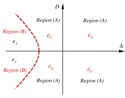
Figure 5: (color online) The ground state eigenvalues as a function of anisotropy and DM coupling. The thick long dashed line which shows the border line of region (A) and region (B) are given by $\Delta=-\sqrt{1+D^{2}}$.

We have considered the three-site block (Fig.(1)) with the following Hamiltonian

$$h_{I}^{B}=\frac{J}{4}\Big{[}(\sigma_{1,I}^{x}\sigma_{2,I}^{x}+\sigma_{2,I}^{x}\sigma_{3,I}^{x}+\sigma_{1,I}^{y}\sigma_{2,I}^{y}+\sigma_{2,I}^{y}\sigma_{3,I}^{y})$$

$$+\Delta(\sigma_{1,I}^{z}\sigma_{2,I}^{z}+\sigma_{2,I}^{z}\sigma_{3,I}^{z})~{}~{}~{}~{}~{}~{}~{}~{}~{}~{}~{}~{}~{}~{}~{}~{}~{}~{}~{}~{}~{}~{}~{}~{}~{}~{}~{}~{}~{}$$

$$+D(\sigma_{1,I}^{x}\sigma_{2,I}^{y}-\sigma_{1,I}^{y}\sigma_{2,I}^{x}+\sigma_{2,I}^{x}\sigma_{3,I}^{y}-\sigma_{2,I}^{y}\sigma_{3,I}^{x})\Big{]}$$

The inter-block ($H^{BB})$ and intra-block ($H^{B}$) Hamiltonian for the three sites decomposition are

$$H^{BB}=\frac{J}{4}\sum_{I}^{N/3}\left[(\sigma_{3,I}^{x}\sigma_{1,I+1}^{x}+\sigma_{3,I}^{y}\sigma_{1,I+1}^{y}+\Delta\sigma_{3,I}^{z}\sigma_{1,I+1}^{z})\right.$$

$$\left.+D(\sigma_{3,I}^{x}\sigma_{1,I+1}^{y}-\sigma_{3,I}^{y}\sigma_{1,I+1}^{x})\right]$$

$$,H^{B}=\frac{J}{4}\sum_{I}^{N/3}\left[(\sigma_{1,I}^{x}\sigma_{2,I}^{x}+\sigma_{2,I}^{x}\sigma_{3,I}^{x}+\sigma_{1,I}^{y}\sigma_{2,I}^{y}+\sigma_{2,I}^{y}\sigma_{3,I}^{y})\right.$$

$$\left.+\Delta(\sigma_{1,I}^{z}\sigma_{2,I}^{z}+\sigma_{2,I}^{z}\sigma_{3,I}^{z})\right.~{}~{}~{}~{}~{}~{}~{}~{}~{}~{}~{}~{}~{}~{}~{}~{}~{}~{}~{}~{}~{}~{}~{}~{}~{}~{}~{}~{}~{}$$

$$\left.+D(\sigma_{1,I}^{x}\sigma_{2,I}^{y}-\sigma_{1,I}^{y}\sigma_{2,I}^{x}+\sigma_{2,I}^{x}\sigma_{3,I}^{y}-\sigma_{2,I}^{y}\sigma_{3,I}^{x})\right].$$

where $\sigma_{j,I}^{\alpha}$ refers to the $\alpha$-component of the Pauli matrix at site $j$ of the block labeled by $I$. The exact treatment of this Hamiltonian leads to four distinct eigenvalues which are doubly degenerate. The ground, first, second and third excited state energies have the following expressions in terms of the coupling constants.

$$|\psi_{0}\rangle=\frac{1}{\sqrt{2q(q+\Delta)(1+D^{2})}}\Big{[}2(D^{2}+1)|\downarrow\downarrow\uparrow\rangle-(1-iD)(\Delta+q)|\downarrow\uparrow\downarrow\rangle-2[2iD+(D^{2}-1)]|\uparrow\downarrow\downarrow\rangle\Big{]},$$ (7)

$$|\psi_{0}^{\prime}\rangle=\frac{1}{\sqrt{2q(q+\Delta)(1+D^{2})}}\Big{[}2(D^{2}+1)|\downarrow\uparrow\uparrow\rangle-(1-iD)(\Delta+q)|\uparrow\downarrow\uparrow\rangle-2[2iD+(D^{2}-1)]|\uparrow\uparrow\downarrow\rangle)\Big{]},$$

$$e_{0}=-\frac{J}{4}(\Delta+q),~{}~{}~{}~{}~{}~{}~{}~{}~{}~{}~{}~{}~{}~{}~{}~{}~{}~{}~{}~{}~{}~{}~{}~{}~{}~{}~{}~{}~{}~{}~{}~{}~{}~{}~{}~{}~{}~{}~{}~{}~{}~{}~{}~{}~{}~{}~{}$$ (8)

$$|\psi_{1}\rangle=\frac{1}{\sqrt{2q(q-\Delta)(1+D^{2})}}\Big{[}2(D^{2}+1)|\downarrow\downarrow\uparrow\rangle-(1-iD)(\Delta-q)|\downarrow\uparrow\downarrow\rangle-2[2iD+(D^{2}-1)]|\uparrow\downarrow\downarrow\rangle\Big{]},$$

$$|\psi_{1}^{\prime}\rangle=\frac{1}{\sqrt{2q(q-\Delta)(1+D^{2})}}\Big{[}2(D^{2}+1)|\downarrow\uparrow\uparrow\rangle-(1-iD)(\Delta-q)|\uparrow\downarrow\uparrow\rangle-2[2iD+(D^{2}-1)]|\uparrow\uparrow\downarrow\rangle)\Big{]},$$

$$e_{0}=-\frac{J}{4}(\Delta-q),~{}~{}~{}~{}~{}~{}~{}~{}~{}~{}~{}~{}~{}~{}~{}~{}~{}~{}~{}~{}~{}~{}~{}~{}~{}~{}~{}~{}~{}~{}~{}~{}~{}~{}~{}~{}~{}~{}~{}~{}~{}~{}~{}~{}~{}~{}~{}$$

$$|\psi_{2}\rangle=\frac{1}{\sqrt{2}(1+D^{2})}\Big{[}[2iD+(D^{2}-1)]|\uparrow\downarrow\downarrow\rangle+(D^{2}-1)|\downarrow\downarrow\uparrow\rangle\Big{]},~{}~{}~{}~{}~{}~{}~{}~{}~{}~{}~{}~{}~{}~{}~{}~{}~{}~{}~{}~{}~{}~{}~{}~{}$$

$$|\psi_{2}^{\prime}\rangle=\frac{1}{\sqrt{2}(1+D^{2})}\Big{[}[2iD+(D^{2}-1)]|\uparrow\uparrow\downarrow\rangle+(D^{2}-1)|\downarrow\uparrow\uparrow\rangle\Big{]},~{}~{}~{}~{}~{}~{}~{}~{}~{}~{}~{}~{}~{}~{}~{}~{}~{}~{}~{}~{}~{}~{}~{}~{}$$

$$e_{2}=0,~{}~{}~{}~{}~{}~{}~{}~{}~{}~{}~{}~{}~{}~{}~{}~{}~{}~{}~{}~{}~{}~{}~{}~{}~{}~{}~{}~{}~{}~{}~{}~{}~{}~{}~{}~{}~{}~{}~{}~{}~{}~{}~{}~{}~{}~{}~{}~{}~{}~{}~{}~{}~{}~{}~{}$$ (9)

$$|\psi_{3}\rangle=|\uparrow\uparrow\uparrow\rangle~{}~{}~{},~{}~{}~{}|\psi_{3}^{\prime}\rangle=|\downarrow\downarrow\downarrow\rangle,~{}~{}~{}~{}~{}~{}~{}~{}~{}~{}~{}~{}~{}~{}~{}~{}~{}~{}~{}~{}~{}~{}~{}~{}~{}~{}~{}~{}~{}~{}~{}~{}~{}~{}~{}~{}~{}~{}~{}~{}~{}~{}~{}~{}$$

$$e_{3}=\frac{J}{2}(\Delta),~{}~{}~{}~{}~{}~{}~{}~{}~{}~{}~{}~{}~{}~{}~{}~{}~{}~{}~{}~{}~{}~{}~{}~{}~{}~{}~{}~{}~{}~{}~{}~{}~{}~{}~{}~{}~{}~{}~{}~{}~{}~{}~{}~{}~{}~{}~{}~{}~{}~{}~{}~{}~{}~{}~{}~{}$$

where $q$ is $q=\sqrt{\Delta^{2}+8(1+D^{2})}$.

$|\uparrow\rangle$ and $|\downarrow\rangle$ are the eigenstates of $\sigma^{z}$. In Fig.(5) we have presented the different regions where the specified state is the ground state of the block Hamiltonian. In the region (A) the projection operator is

$$P_{0}=|\Uparrow\rangle\langle\psi_{0}|+|\Downarrow\rangle\langle\psi_{0}^{\prime}|.$$

The Pauli matrices in the effective Hilbert space have the following transformations

$$P_{0}^{I}\sigma_{1,I}^{x}P_{0}^{I}=-\frac{2}{q}({\sigma^{\prime}}_{I}^{x}+D{\sigma^{\prime}}_{I}^{y})~{}~{}~{},~{}~{}~{}P_{0}^{I}\sigma_{2,I}^{x}P_{0}^{I}=\frac{4(D^{2}+1)}{q(\Delta+q)}{\sigma^{\prime}}_{I}^{x}~{}~{}~{},~{}~{}~{}P_{0}^{I}\sigma_{3,I}^{x}P_{0}^{I}=-\frac{2}{q}({\sigma^{\prime}}_{I}^{x}-D{\sigma^{\prime}}_{I}^{y})$$

$$P_{0}^{I}\sigma_{1,I}^{y}P_{0}^{I}=-\frac{2}{q}(D{\sigma^{\prime}}_{I}^{x}-{\sigma^{\prime}}_{I}^{y})~{}~{}~{},~{}~{}~{}P_{0}^{I}\sigma_{2,I}^{y}P_{0}^{I}=-\frac{4(D^{2}+1)}{q(\Delta+q)}{\sigma^{\prime}}_{I}^{y}~{}~{}~{},~{}~{}~{}P_{0}^{I}\sigma_{3,I}^{y}P_{0}^{I}=\frac{2}{q}(D{\sigma^{\prime}}_{I}^{x}+{\sigma^{\prime}}_{I}^{y})$$

$$P_{0}^{I}\sigma_{1,I}^{z}P_{0}^{I}=P_{0}^{I}\sigma_{3,I}^{z}P_{0}^{I}=-\frac{\Delta+q}{2q}{\sigma^{\prime}}_{I}^{z}~{}~{}~{},~{}~{}~{}P_{0}^{I}\sigma_{2,I}^{z}P_{0}^{I}=\frac{\Delta}{q}{\sigma^{\prime}}_{I}^{z}~{}~{}~{}~{}~{}~{}~{}~{}~{}~{}~{}~{}~{}~{}~{}~{}~{}~{}~{}~{}~{}~{}~{}$$

In the region (B) ($\Delta<-\sqrt{1+D_{2}}$) the projection operator is

$$P_{0}=|\Uparrow\rangle\langle\psi_{3}|+|\Downarrow\rangle\langle\psi_{3}^{\prime}|.$$

and the Pauli matrices in the effective Hilbert space have the following transformations

$$P_{0}^{I}\sigma_{1,I}^{x}P_{0}^{I}=0~{}~{}~{},~{}~{}~{}P_{0}^{I}\sigma_{2,I}^{x}P_{0}^{I}=0~{}~{}~{},~{}~{}~{}P_{0}^{I}\sigma_{3,I}^{x}P_{0}^{I}=0$$

$$P_{0}^{I}\sigma_{1,I}^{y}P_{0}^{I}=0~{}~{}~{},~{}~{}~{}P_{0}^{I}\sigma_{2,I}^{y}P_{0}^{I}=0~{}~{}~{},~{}~{}~{}P_{0}^{I}\sigma_{3,I}^{y}P_{0}^{I}=0$$

$$P_{0}^{I}\sigma_{1,I}^{z}P_{0}^{I}=P_{0}^{I}\sigma_{3,I}^{z}P_{0}^{I}=P_{0}^{I}\sigma_{2,I}^{z}P_{0}^{I}={\sigma^{\prime}}_{I}^{z}.$$

V.2 Order Parameter and Chiral Order

V.2.1 Staggered magnetization

Generally, any correlation function can be calculated in the QRG scheme. In this approach, the correlation function at each iteration of RG is connected to its value after an RG iteration. This will be continued to reach a controllable fixed point where we can obtain the value of the correlation function. The staggered magnetization in $\alpha$ direction can be written

$$S_{M}=\frac{1}{N}\sum_{i}^{N}\langle O|\frac{(-1)^{i}}{2}\sigma_{i}^{\alpha}|O\rangle,$$ (10)

where $\sigma_{i}^{\alpha}$ is the Pauli matrix in the $i$th site and $|O\rangle$ is the ground state of chain. The ground state of the renormalized chain is related to the ground state of the original one by the transformation, $P_{0}|O^{\prime}\rangle=|O\rangle$.

$$S_{M}=\frac{1}{N}\sum_{i}^{N}\langle O^{\prime}|P_{0}(\frac{(-1)^{i}}{2}\sigma_{i}^{\alpha})P_{0}|O^{\prime}\rangle.$$

This leads to the staggered configuration in the renormalized chain. The staggered magnetization in $z$ direction is obtained

$$S_{M}^{0} = \frac{1}{N}\sum_{i=1}^{N}\langle 0|\frac{(-1)^{i}}{2}\sigma_{i}^{z}|0\rangle$$ (11)

$$= \frac{1}{6}\frac{1}{\frac{N}{3}}\sum_{I=1}^{N/3}\Big{[}\langle 0^{\prime}|P_{0}^{I}(-\sigma_{1,I}^{z}+\sigma_{2,I}^{z}-\sigma_{3,I}^{z})P_{0}^{I}|0^{\prime}\rangle$$

$$- \langle 0^{\prime}|P_{0}^{I+1}(-\sigma_{1,I+1}^{z}+\sigma_{2,I+1}^{z}-\sigma_{3,I+1}^{z})P_{0}^{I+1}|0^{\prime}\rangle\Big{]}$$

$$= -\frac{2\Delta+q}{3q}\frac{1}{\frac{N}{3}}\sum_{I=1}^{N/3}\langle 0^{\prime}|\frac{(-1)^{i}}{2}\sigma_{I}^{z}|0^{\prime}\rangle=-\frac{\gamma^{0}}{3}S_{M}^{1},$$

where $S_{M}^{(n)}$ is the staggered magnetization at the $n$th step of QRG and $\gamma^{(0)}$ is defined by $\gamma^{0}=(2\Delta+q)/q$.

This process will be iterated many times by replacing $\gamma^{(0)}$ with $\gamma^{(n)}$. The expression for $\gamma^{(n)}$ is similar to $\gamma^{(0)}$ where the coupling constants should be replaced by the renormalized ones at the corresponding RG iteration ($n$). The result of this calculation has been presented in Fig.(3) and Fig.(4).

V.2.2 Chiral Order

The chiral order which is the proper function to detect the helical magnetization in the systems can be written

$$C_{h}=\frac{1}{N}\sum_{i=1}^{N}\frac{1}{4}\langle(\sigma_{i}^{x}\sigma_{i+1}^{y}-\sigma_{i}^{y}\sigma_{i+1}^{x})\rangle.$$ (12)

As we mentioned in the section III, the $XX$ term of the Hamiltonian shows up to the chiral order under RG. The $XX$ term order is written

$$D_{XX}=\frac{1}{N}\sum_{i=1}^{N}\frac{1}{4}\langle(\sigma_{i}^{x}\sigma_{i+1}^{x}+\sigma_{i}^{y}\sigma_{i+1}^{y})\rangle.$$ (13)

In this case the calculating of the chiral order being elaborate, because of the unknown effect of the $XX$ term on the ground state of system at fixed point ($\Delta=\infty$). To simplification of the calculation, we transform the $XXZ$ with DM interaction Hamiltonian (Eq.(1)) to the Ising model with DM interactionJafari2 (IDM) by implement a non-local transformation which shows a $n\varphi$ rotation about the $z$ axis at site $n$ where $\varphi=\arctan(-\frac{1}{D})$. We have calculated the chiral order (Eq.(12)) of IDM in Ref.[Jafari2 ]. By implement the inverse of transformation, the chiral order in IDM model transforms to the DC order where introduced in Eq.(6). The DC order has been plotted in Fig.(3) and Fig.(4) versus $D$ and $\Delta$.

V.3 Classical Approximation

In the classical approximation the spins are considered as classical vectors which form the spiral structure with a pitch angle $\varphi$ between neighboring spins and canted angle $\theta$

$$\sigma^{x}_{n}=\cos(n\varphi)\sin\theta~{}~{},\sigma^{y}_{n}=\sin(n\varphi)\sin\theta~{}~{},\sigma^{z}_{n}=\cos\theta,$$

The classical energy per site for the $XXZ$ with DM interaction Hamiltonian (Eq.(1)) is

$$\frac{E_{cl}}{N}=\frac{J}{4}[(\cos\varphi+D\sin\varphi)\sin^{2}\theta+\Delta\cos^{2}\theta].$$

The minimization of classical energy with respect to the angles $\varphi$ and $\theta$ shows that there are two different regions. (I) $\Delta>\sqrt{1+D^{2}}$, the minimum of energy is obtained by arbitrary $\theta$ and $\varphi=\arctan(D)$ which show the spins projection on $z$ axis is nonzero and spins have the helical structure (see Fig.6) in the $xy$ plain. In this region the minimum classical energy is

$$\frac{E_{cl}^{I}}{N}=\frac{J}{4}(\sqrt{1+D^{2}}\sin^{2}\theta+\Delta\cos^{2}\theta).$$ (14)

(II) $\Delta<\sqrt{1+D^{2}}$, the energy is minimized by $\Delta=\cos\varphi+D\sin\varphi$ and arbitrary $\theta$ or arbitrary $\varphi$ and $\theta=\frac{\pi}{2}$, which correspond respectively to the configurations with nonzero value of spins projection on $z$-axis with helical structure of spins projection in the $xy$-plain and disorder configuration. In this region the minimum classical energy is

$$\frac{E_{cl}^{II}}{N}=\frac{J}{4}(\cos\varphi+D\sin\varphi)=\frac{J}{4}\Delta.$$ (15)

One can see from Eq.(14) and Eq.(15) that the transition between phase (I) and (II) takes place at $\Delta=\sqrt{1+D^{2}}$.

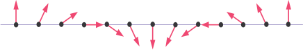
Figure 6: (color online) A classical picture of spin orientation in the $xy$ plain where the angle between neibouring spins depend on the D value.

VI Canonical Transformation

The Hamiltonian of $XXZ$ model with DM interaction (Eq.(1)) has the global $U(1)\times Z_{2}$ symmetry. This Hamiltonian is mapped to the well known $XXZ$ chain via a canonical transformationAristov ; Alcaraz ,

$$U=\sum_{j=1}^{N}\alpha_{j}\sigma_{j}^{z}~{}~{}~{} ~{}~{}~{}\alpha_{j}=\sum^{j-1}_{m=1}m\tan^{-1}(D),$$ ,

$$\tilde{\sigma}^{\pm}_{j}=e^{-iU}\sigma^{\pm}_{j}e^{iU} ~{}~{}~{}~{}~{}\tilde{\sigma}^{z}_{j}=\sigma^{z},$$ ,

$$\tilde{H} = e^{-iU}He^{iU},$$ (16)

which gives

$$\tilde{H}=\frac{J\sqrt{1+D^{2}}}{4}\Big{[}\sum_{i}\tilde{\sigma}^{x}_{i}\tilde{\sigma}^{x}_{i+1}+\tilde{\sigma}^{y}_{i}\tilde{\sigma}^{y}_{i+1}+(\frac{\Delta}{\sqrt{1+D^{2}}})\tilde{\sigma}^{z}_{i}\tilde{\sigma}^{z}_{i+1}\Big{]}.$$ (17)

The $U(1)\times Z_{2}$ symmetry of initial Hamiltonian survive in the transformed Hamiltonian too, but at $\Delta_{c}=\pm\sqrt{1+D^{2}}$ the $U(1)\times Z_{2}$ symmetry breaks to the local $SU(2)$ symmetry.

References

References

(1)
M. Vojta, Rep. Prof. Phys. 66, 2069 (2003) and references
therein.
(2)
I. Dzyaloshinskii, J. Phys. Chem. Solids 4, 241 (1958).
(3)
T. Moriya, Phys. Rev 120, 91 (1960).
(4)
P. W. Anderson, Phys. Rev 115, 2 (1959).
(5)
D. Coffey, K. S. Trugman, Phys. Rev. B. 42, 6509 (1990).
(6)
D. C. Dender, P. R. Hammar,D. H. Reich, C. Broholm , and G. Aeppli
Phys. Rev. Lett 79, 1750 (1997).
(7)
M. Oshikawa, I. Affleck, Phys. Rev. Lett 79, 2883 (1997).
(8)
J. Z. Zhao, X. Q. Wang, T. Xiang, Z. B. Su, L. Yu, Phys. Rev. Lett
90, 20204 (2003).
(9)
J.-B. Fouet, O. Tchernyshyov, F. Mila, Phys. Rev. B. 70,
174427 (2004); J.-B. Fouet, F. Mila, D. Clarke, H. Youk, O.
Tchernyshyov. P.Fendley, R. M. Noack, Phys. Rev. B. 73,
214405 (2006).
(10)
A. L. Chernyshev, Phys. Rev. B. 72, 174414 (2005).
(11)
D. C. Dender, D. Dvidovic, D. H. Reich, C. Broholm , and G. Aeppli
Phys. Rev. B 53, 2583 (1996).
(12)
M. Kohgi, K. Iwasa, J. Mignot, B. Fak, P. Gegenwart, M. Lang, A.
Ochiai, H. Aoki, and T. Suzuki, Phys. Rev. Lett 86, 2439
(2000).
(13)
P. Fulde B. Schmidt, and P. Thalmeier, Europhys. Lett 31,
323 (1995).
(14)
M. Oshikawa, K. Ueda, H. Aoki, A. Ochiai and M. Kohgi, J. Phys. Soc.
Jpn 68, 3181 (1999); H. Shiba, K. Udea, and O. Sakai, J.
Phys. Soc. Jpn 69, 1493 (2000)
(15)
I. Tsukada, J. T. Takeya, T. Masuda and K. Uchinokura, Phys. Rev.
Lett 87, 127203 (2001)
(16)
b. Grande and Hk. Mller-Buschbaum, Z. Anorg. Allg. Chem
417, 68 (1975).
(17)
M. Greven, R. J. Birgeneau, Y. Endoh, M. A. Kastner, M. Matsuda, and
G. Shirane, Z. Phys. B 96, 465 (1995).
(18)
A. B. Harris, A. Aharony and O. E. Wohlman, Phys. Rev. B.
52, 10239 (1995).
(19)
K. Katsumata, M. Hagiwara,Z. Honda, J. Satooka, A. Aharoy, R. J.
Birgeneau, F. C. Chou, O. E. Wohlman, A. B. Harris,M. A. Kastner, Y.
J. Kim, and Y. S. Lee, Europhys. Rev. Lett 54, 508(2001).
(20)
M. A. Kastner, R. J. Birgeneau, G. Shirane and Y. Endoh, Rev. Mod.
Phys 70, 897 (1998).
(21)
M. A. Martin-Delgado and G. Sierra, Int. J. Mod, Phys. A
11, 3145 (1996).
(22)
G. Sierra and M. A. Martin Delgado, in Strongly Correlated
Magnetic and Superconducting Systems, Lecture Notes in Physics Vo1.
478 (springer, Berlin, 1997).
(23)
A. Langari, Phys. Rev. B 58, 14467 (1998); it ibid 69,
100402(R) (2004).
(24)
R. Jafari, A. Langari, Phys. Rev. B 76, 014412 (2007);
R. Jafari, A. Langari, Physica A 364, 213 (2006).
(25)
F. C. Alcaraz and W. F. Wreszinski, J. Stat. Phys. 58, 45
(1990).
(26)
H. Kawamura, Phys. Rev. B 38, 4916 (1988).
(27)
M. Kaburagi, and H. Kawamura, T. Hikihara, J. Phys. Soc. Jpn.
68, 3185 (1999);T. Hikihara, M. Kaburagi, and H.
Kawamura, arXiv:cond-mat/0007095v2; T. Hikihara, M. Kaburagi, and
H. Kawamura, arXiv:cond-mat/0010283v1.
(28)
R. Jafari, M. Kargarian, A. Langari, and M. Siahatgar, Phys. Rev.
B , (2008).
(29)
D. N. Aristov, S. V. Maleyev, Phys. Rev. B 62, R751