UNAVERAGED THREE-DIMENISONAL MODELLING OF THE FEL

Abstract

A new three-dimensional model of the FEL is presented. A system of scaled, coupled Maxwell–Lorentz equations are derived in the paraxial limit. A minimal number of limiting assumptions are made and the equations are not averaged in the longitudinal direction of common radiation/electron beam propagation, allowing the effects of coherent spontaneous emission and non-localised electron propagation to be modelled. The equations are solved numerically using a parallel Fourier split-step method.

1 INTRODUCTION

A three-dimensional model of a helical wiggler Free Electron Laser (FEL) is presented that minimises the assumptions made. This model does not average the Maxwell–Lorentz equations describing the interaction between the electrons, wiggler and radiation fields. Furthermore, no relativistic approximations in the equations governing electron motion are made and transverse motion of the electrons is self-consistently driven by both the wiggler and radiation fields. Current 3D codes perform averaging over a radiation wavelength of the radiation and others also over the the electron trajectories. Thus no study of the effects of coherent spontaneous emission (CSE) or self amplified coherent spontaneous emission (SACSE) is possible. Furthermore, these codes cannot model large energy losses by the electrons as the electrons are confined locally to a wavelength. In this model no such averaging is done and so sub-period radiation evolution is included and electron migration over distances greater than a wavelength, for example due to locally high radiation powers, may be described.

2 3D MODEL

Following the method of previous studies for the one-dimensional FEL [1, 3, 2] the physics of the FEL may be described in three dimensions by the coupled Maxwell–Lorentz equations

$$\left(\nabla^{2}-\frac{1}{c^{2}}\frac{\partial^{2}}{\partial t^{2}}\right)\mathbf{E}(\mathbf{r},t)=\mu_{0}\frac{\partial\mathbf{J}_{\perp}(\mathbf{r},t)}{\partial t}$$ (1)

$$\frac{d\mathbf{p}_{j}}{dt}=-e\left(\mathbf{E}(\mathbf{r}_{j},t)+\frac{\mathbf{p}_{j}}{\gamma_{j}m}\times\mathbf{B}(\mathbf{r}_{j},t)\right)$$ (2)

where $j=1\ldots N$, the total number of electrons, and the transverse current density may be written

$$\mathbf{J}_{\perp}(\mathbf{r},t)=-\frac{e}{m}\sum_{j=1}^{N}\frac{\bar{p}_{\perp j}}{\gamma_{j}}\delta(\mathbf{\bar{r}}-\mathbf{\bar{r}}_{j}(t)),$$ (3)

where $m$ is the electron rest mass. The helical wiggler and radiation electric field are assumed to be

$${\bf B}_{w}(\mathbf{r}) = \frac{B_{w}}{\sqrt{2}}(\hat{\bf{e}}\,e^{-ik_{w}z}+c.c.)$$

$$+\frac{B_{w}k_{w}}{2}[ix(e^{-ik_{w}z}-c.c.)+y(e^{ik_{w}z}+c.c.)]\hat{\bf{z}}$$

$${\bf E}(\mathbf{r},t) = \frac{1}{\sqrt{2}}(\hat{\bf{e}}\;\xi_{0}({\bf r},t)e^{i(kz-\omega t)}+c.c.)$$ (5)

where $\hat{\bf{e}}=(\hat{\bf{x}}+i\hat{\bf{y}})/\sqrt{2}$, $\xi_{0}$ is a slowly varying complex field envelope and $B_{w}$ is the wiggler magnetic field strength of period $\lambda_{w}=2\pi/k_{w}$. The magnetic component of the radiation field $\mathbf{B}(\mathbf{r},t)$ is required in the Lorentz equation and may be calculated from Maxwell’s equations to give:

$$\mathbf{B}(\mathbf{r},t)=-\frac{i}{\sqrt{2}}\left(\frac{\xi_{0}({\bf r},t)}{c}\;\hat{\bf{e}}\,e^{i(kz-\omega t)}-c.c.\right)$$ (6)

where it has been assumed that any radiation that is counter-propagating the electron beam may be neglected. The following scaling notation is now introduced:

$$\varepsilon Q_{j} = \frac{1-\beta_{z_{j}}}{\beta_{z_{j}}},\varepsilon=\frac{1-\bar{\beta}_{z}}{\bar{\beta}_{z}},\alpha=\left(\frac{2\rho\gamma_{r}}{a_{w}}\right)^{2},$$

$$\bar{p}_{\perp} = \frac{p_{x}-ip_{y}}{mc},A=\frac{e\xi_{0}}{mc\omega_{p}\sqrt{\gamma_{r}\rho}},$$

$$\bar{z} = 2k_{w}\rho z,\ \bar{z}_{2}=2k_{w}\rho\frac{\bar{\beta}_{z}}{1-\bar{\beta}_{z}}(ct-z),$$

$$\bar{x} = \frac{x}{\sqrt{l_{g}l_{c}}},\ \bar{y}=\frac{y}{\sqrt{l_{g}l_{c}}}$$

where $\bar{\beta}_{z}=v_{z0}/c$ is the mean electron velocity on entering the interaction region, $\gamma_{r}$ is the resonant electron energy and $\rho$ is the fundamental FEL parameter, defined as

$$\rho=\frac{1}{\gamma_{r}}\left(\frac{a_{w}\omega_{p}}{4ck_{w}}\right)^{2/3}.$$

Here $\omega_{p}=\sqrt{e^{2}n_{p}/(\varepsilon_{0}m)}$ is the plasma frequency for the peak electron number density of the electron pulse $n_{p}$, and $a_{w}=eB_{w}/(mck_{w})$ is the wiggler deflection parameter. The scaled electron density is defined as $\bar{n}_{p}=n_{p}l_{g}l_{c}^{2}$, where $l_{g}$ is the gain length and $l_{c}$ the cooperation length. Note the scaling in the transverse plane is with respect to the physically relevant gain and cooperation lengths. This allows the equations above describing the FEL interaction to be written as

$$-i\rho\left(\frac{\partial^{2}A}{\partial\bar{x}^{2}}+\frac{\partial^{2}A}{\partial\bar{y}^{2}}\right)+\frac{\partial A}{\partial\bar{z}}+2i\rho\frac{\partial^{2}A}{\partial\bar{z}\partial\bar{z}_{2}}=$$

$$\frac{\gamma_{r}}{a_{w}}\frac{1}{\bar{n}_{p}}\sum_{j=1}^{N}\frac{\bar{p}_{\perp j}(\varepsilon Q_{j}(\varepsilon Q_{j}+2))^{1/2}}{(1+|\bar{p}_{\perp j}|^{2})^{1/2}}\delta(\mathbf{\bar{r}}-\mathbf{\bar{r}_{j}})e^{i\frac{\bar{z}_{2j}}{2\rho}}$$

$$\frac{d\bar{p}_{\perp j}}{d\bar{z}} = \frac{a_{w}}{2\rho}\left[ie^{-i\frac{\bar{z}}{2\rho}}-\alpha\varepsilon Q_{j}Ae^{-i\frac{\bar{z}_{2j}}{2\rho}}\right]-$$

$$\mbox{}\frac{a_{w}^{2}\varepsilon}{8\rho^{2}}\sqrt{\frac{Q_{j}(2+\varepsilon Q_{j})}{(1+|\bar{p}_{\perp j}|^{2})}}\frac{(\bar{x}_{j}-i\bar{y}_{j})}{(1+\varepsilon Q_{j})^{2}}$$

$$\frac{dQ_{j}}{d\bar{z}} = \frac{a_{w}}{4\rho}\frac{Q_{j}(\varepsilon Q_{j}+2)}{1+|\bar{p}_{\perp j}|^{2}}\times$$ (9)

$$\left[i(\varepsilon Q_{j}+1)(\bar{p}_{\perp j}^{*}e^{-i\frac{\bar{z}}{2\rho}}-c.c.)+\right.$$

$$\left.\alpha\varepsilon Q_{j}(\bar{p}_{\perp j}^{*}Ae^{-i\frac{\bar{z}_{2j}}{2\rho}}+c.c.)\right]$$

$$\frac{d\bar{z}_{2j}}{d\bar{z}} = Q_{j}$$ (10)

$$\frac{d\bar{x}_{j}}{d\bar{z}} = \Re(\bar{p}_{\perp j})\sqrt{\frac{Q_{j}(2+\varepsilon Q_{j})}{1+|\bar{p}_{\perp j}|^{2}}}$$ (11)

$$\frac{d\bar{y}_{j}}{d\bar{z}} = -\Im(\bar{p}_{\perp j})\sqrt{\frac{Q_{j}(2+\varepsilon Q_{j})}{1+|\bar{p}_{\perp j}|^{2}}}$$ (12)

In deriving the equations the only approximations made are the neglect of space charge and the paraxial approximation. There are no restrictions on the electron energy allowing large changes to be modelled.

In the scaled variables used here, the normalised beam emittance is given by

$$\epsilon_{n}=\sqrt{l_{g}l_{c}}\sigma_{\bar{x}}\sigma_{\bar{p}_{x}}.$$ (13)

For an electron beam matched to a focussing channel the radius of the electron beam envelope is given by

$$r_{b}=\left(\frac{\epsilon_{n}\beta}{\gamma_{r}}\right)^{1/2}.$$ (14)

The electrons experience a natural focussing force due to the magnetic field of the helical wiggler [4] resulting in a beta-function of $\beta=\gamma_{r}/a_{w}k_{w}$. This restoring force is approximated by the final linear term in (2) and may be simply modified in magnitude to approximate other, e.g. FODO, focussing channels.

The scaled Rayleigh range (in units of $\bar{z}$) can be shown to be $\bar{z}_{R}=\sigma_{\bar{r}}^{2}/2\rho$, where $\sigma_{\bar{r}}$ is the radius of the beam in scaled units of $\bar{x},\bar{y}$.

It can be shown that the above equations satisfy energy conservation, written in the form:

$$\underbrace{\int\int\int}_{allspace}|A|^{2}d\bar{x}\;d\bar{y}\;d\bar{z}_{2}+\frac{1}{\gamma_{r}\rho}\sum_{k=1}^{N_{p}}\bar{\chi}_{k}\gamma_{k}=0$$ (15)

$$\mbox{ where }\gamma_{k}=\sqrt{\frac{(1+|\bar{p}_{\perp k}|^{2})(1+\varepsilon Q_{k})^{2}}{\varepsilon Q_{k}(\varepsilon Q_{k}+2)}}$$

which may be used as a check in the numerical solution.

In the relativistic Compton limit $\epsilon,\rho\ll 1$ the above equations can be shown to reduce to those of [1].

3 NUMERICAL SOLUTION

The field evolution of the scaled equations (2)–(12) are solved by applying a modified parallel Fourier split-step method [5] in conjunction with a finite element method [6]. This allows the effects of coherent spontaneous emission (CSE), self-amplified spontaneous emission (SASE) and diffraction to be modelled numerically. The parallel code was developed using the Numerical Algorithms Group (NAG) parallel routines to control the parallel processing. The Fourier split-step method involves solving the wave equation in two steps. The first step considers the field diffracting in the transverse direction and propagating in the $\bar{z}$ direction freely without the electron source term:

$$-i\rho\left(\frac{\partial^{2}A}{\partial\bar{x}^{2}}+\frac{\partial^{2}A}{\partial\bar{y}^{2}}\right)+\frac{\partial A}{\partial\bar{z}}+2i\rho\frac{\partial^{2}A}{\partial\bar{z}\partial\bar{z}_{2}}=0.$$ (16)

This equation can be solved by taking the Fourier transforms in $\bar{x}$, $\bar{y}$ and $\bar{z}_{2}$ resulting in an ordinary differential equation in the Fourier transformed field $\tilde{A}$, with the following analytic solution:

$$\tilde{A}(\bar{z}+\Delta\bar{z})=\tilde{A}(\bar{z})\exp\left[\frac{-i\rho k_{\perp}^{2}}{(1-2\rho k_{\bar{z}_{2}})}\Delta\bar{z}\right],$$ (17)

where the transverse Fourier transform variable pairs are given by $(\bar{x},k_{\bar{x}})$, $(\bar{y},k_{\bar{y}})$, $(\bar{z}_{2},k_{\bar{z}_{2}})$ and $k_{\perp}^{2}=k_{\bar{x}}^{2}+k_{\bar{y}}^{2}$. The inverse numerical Fourier transform is then applied giving solution $A(\bar{x},\bar{y},\bar{z}_{2},\bar{z}+\Delta\bar{z})$ which is then used as the initial field for the second part of the split-step method where the diffraction terms are neglected and the source term acts alone:

$$\frac{\partial A}{\partial\bar{z}}+2i\rho\frac{\partial^{2}A}{\partial\bar{z}\partial\bar{z}_{2}}=$$ (18)

$$\frac{\gamma_{r}}{a_{w}}\frac{1}{\bar{n}_{p}}\sum_{j=1}^{N}\frac{\bar{p}_{\perp j}(\varepsilon Q_{j}(\varepsilon Q_{j}+2))^{1/2}}{(1+|\bar{p}_{\perp}|^{2})_{j}^{1/2}}\delta(\mathbf{\bar{r}}-\mathbf{\bar{r}_{j}})e^{i\frac{\bar{z}_{2j}}{2\rho}}.$$

The finite element method is then used to solve the wave equations (18) and (2)–(12) along with a fourth order Runge-Kutta method for electron variables to give the final solution.

Before applying the finite element method to the wave equation, the summation over the real electrons has to be changed to a summation over a group of macroparticles, each of which represents many real electrons. This reduces the computational memory load and operation:

$$\frac{1}{\bar{n}_{p}}\sum_{j=1}^{N}(\cdots)_{j}=\frac{1}{\bar{n}_{p}}\sum_{k=1}^{N_{p}}N_{k}(\cdots)_{k}$$ (19)

where subscripts $j$ and $k$ indicate evaluation at the particle position, $N_{p}$ is the total number of macroparticles and $N_{k}$ is the charge weight of the macroparticle in units of the electron charge.

The Galerkin method of the finite elements is used. The field is described by a set of 8-node hexahedral elements with linear basis functions $\Lambda_{m}(\bar{x},\bar{y},\bar{z}_{2})$ and nodal values $a_{m}(\bar{z})$:

$$A(\bar{x},\bar{y},\bar{z},\bar{z}_{2})=\sum_{m}a_{m}(\bar{z})\Lambda_{m}(\bar{x},\bar{y},\bar{z}_{2}).$$ (20)

where $m$ is the global node index of the 3D system. Note that $\Lambda_{m}(\bar{x},\bar{y},\bar{z}_{2})\equiv 0$ outwith the elements to which it belongs. The wave equation (18) then reduces to a matrix equation for the nodal points:

$${\bf K}\frac{\partial a_{m}(\bar{z})}{\partial\bar{z}}=\frac{\gamma_{r}}{a_{w}}\sum_{k=1}^{N_{p}} \frac{\bar{\chi}_{k}}{V_{e}}\frac{\bar{p}_{\perp k}(\varepsilon Q_{k}(\varepsilon Q_{k}+2))^{1/2}}{(1+|\bar{p}_{\perp}|^{2})^{1/2}}\times$$

$$\Lambda_{m}(\bar{x}_{k},\bar{y}_{k},\bar{z}_{2k})e^{i\frac{\bar{z}_{2k}}{2\rho}}$$

where $\bf K$ is the stiffness matrix constructed from the elemental equations [6], $\bar{\chi}$ is a macroparticle weighting function and $V_{e}$ is the scaled volume of an element of the system, $V_{e}=\Delta\bar{x}\Delta\bar{y}\Delta\bar{z}_{2}$.

4 A SIMULATION IN THE 1D LIMIT

To test the 3D model a comparison with the 1D results of [1, 2] was made. In these one-dimensional models the wave equation was integrated analytically over the common electron/radiation transverse area before numerical solutions were obtained.

Here, one element is used in the transverse plane approximating the radiation field to a plane wave and allowing integration over the transverse area and comparison with the 1D results. The electron beam radius was set greater than the electron orbital radius ensuring the electron beam does not move significantly in the transverse plane of the element. A gaussian distribution for the electrons in the transverse plane was used with a range of six times the standard deviation. The results of [1] Fig. 2 showing self-amplified coherent spontaneous emission (SACSE) for a top-hat pulse current are reproduced in Fig. 1. (Note that there is a scale reversal as [1] plots the power as a function of $\bar{z}_{1}$ while here it is plotted as a function of $\bar{z}_{2}$.)

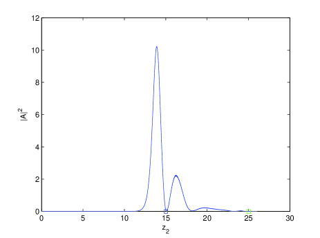
Figure 1: The scaled radiation power $|A|^{2}$ as a function of $\bar{z}_{2}$ demonstrating good agreement with the 1D model of  [1] Fig. 2

The coherent spontaneous emission, including the effects of shot noise, from both square and gaussian shaped pulses of [2] were also reproduced. In Fig. 2 the top hat case of [2] Fig. 4 is plotted.

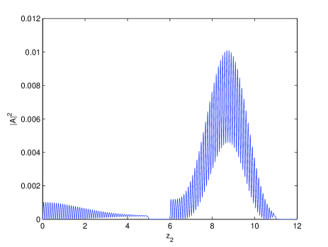
Figure 2: The scaled radiation power $|A|^{2}$ as a function of $\bar{z}_{2}$ demonstrating good agreement with the 1D model of [2] Fig. 4

Good agreement between the 1D models of [1, 2] and the 1D limit of the 3D model of this paper are observed.

5 A SIMULATION IN 3D

An example of the code operating in 3D is now presented. The parameters used are not intended to model any specific system, but rather to demonstrate the functioning of the code and its associated post-processing and plotting routines. A relatively simple system was chosen with a short electron pulse so that coherent spontaneous effects can be observed and large computational effort is not required.

The energy spread and the emittance of the beam were set to zero, the emittance by setting $\sigma_{\bar{p}_{x,y}}=0$ for all electrons. Focussing was therefore not required for this simulation. The code was run using 16-processors of a parallel computer with parameters shown in Table 1.

Electron beam parameters
Energy  E	$250$ MeV
Bunch Charge  Q	$100$ pC
Peak Intensity  $I_{pk}$	$\sim 9394$A
Distribution in $\bar{x}\ \&\ \bar{y}$	Gaussian
Sigma in $\bar{x},\bar{y}$  $\sigma_{\bar{x},\bar{y}}$	$\sim 0.228$
Distribution in $\bar{z}_{2}$	Top-hat
Length of pulse in $\bar{z}_{2}$	$1.5$
Emittance and energy spread	0
Undulator parameters
Undulator Type	Helical
Pierce parameter  $\rho$	$\sim 1.5$e$-2$
Wiggler deflection parameter  $a_{w}$	$1.5$
Propagation distance  $\bar{z}$	$5.00$
Radiation parameters
Initial seed field over pulse  $A_{0}$	0.01
Seed distribution in $\bar{x}\ \&\ \bar{y}$	Gaussian
Sigma in $\bar{x},\bar{y}$  $\sigma_{\bar{x},\bar{y}}$	$\sim 0.228$
Rayleigh length  $\bar{z}_{R}$	1.74
Distribution of seed in $\bar{z}_{2}$	Top-hat
Length of seed in $\bar{z}_{2}$	$1.5$

Table 1: 3D parameters

Fig. 3 plots the scaled intensity $|A|^{2}$ across a transverse slice at the head of the electron pulse, just as the radiation escapes to propagate into vacuum. In Fig. 4 the scaled power ($|A|^{2}$ integrated across the transverse plane) is plotted as a function of $\bar{z}_{2}$ following a FEL interaction to $\bar{z}=5$. Both plots demonstrate the main features of FEL interaction with Coherent Spontaneous Emission and the energy conservation relation of (15) is confirmed to within 0.5%.

Further testing of the code is being carried out and will be reported upon in a future publication.

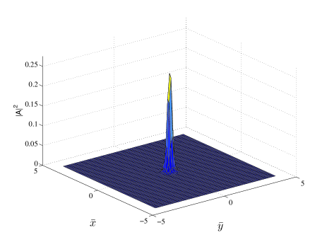
Figure 3: The scaled radiation intensity $|A|^{2}$ in the transverse $(\bar{x},\bar{y})$ plane at $\bar{z}=5$. The transverse slice is taken at the ‘head’ of the electron pulse at $\bar{z}_{2}=5$.

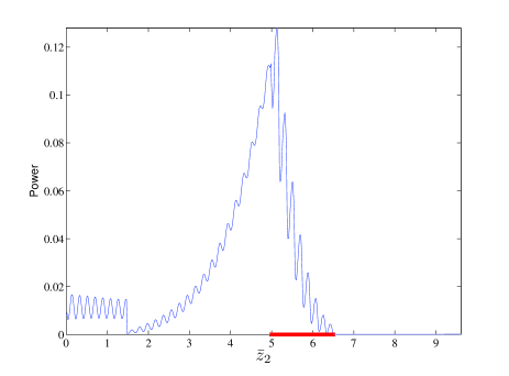
Figure 4: The scaled radiation power at $\bar{z}=5$ as a function of $\bar{z}_{2}$. The electron pulse is shown on the $\bar{z}_{2}$ axis lying between $5<\bar{z}_{2}<6.5$. In this frame the electron pulse propagates along $\bar{z}_{2}$ with increasing $\bar{z}$.

6 CONCLUSION

A new parallel code has been developed which models the FEL amplifier by solving a system of scaled equations describing the FEL interaction in three spatial and the time dimension. The aim has been to introduce as few approximations into the model as possible, the main assumptions being the neglect of space charge and any backward propagating radiation fields. This allows the effects of coherent spontaneous emission, diffraction and full electron transport throughout the region of integration to be modelled. Furthermore, the sub-wavelength discretisation of the model allows a significantly wider range of radiation frequencies to be modelled than is possible with most other codes that use a minimum discretisation interval of a radiation wavelength. A 1D limit of the computational model was identified and simulation results in this limit show agreement with previous 1D numerical and analytical models. A further example simulation has been presented which demonstrates the code operating successfully using an electron pulse in three dimensions. Further optimisation of the code is ongoing. While the code is undoubtedly slower to operate than other 3D averaged codes, the extended physics that it can model may be expected to yield interesting new phenomena in FEL physics.

References

- [1] B.W.J. McNeil, G.R.M. Robb and D.A. Jaroszynski, Opt. Commun.165 (1999) 65
- [2] B.W.J. McNeil, M.W. Poole and G.R.M. Robb, Phys. Rev. ST Accel. Beams , 070701 (2003)
- [3] B.W.J. McNeil, G.R.M. Robb and M.W. Poole, Proceedings of the 2003 Particle Accelerator Conference, p953 Vol.2
- [4] E.T. Scharlemann, ’Selected Topics in FELs’, High Gain, High Power Free Electron Laser, R. Bonifacio, L.De Salvo and C. Pellegrini (editors) (1989) 95
- [5] R. H. Hardin and F.D. Tappert, Applications of the split-step Fourier method to the numerical solution of nonlinear and variable coefficient wave equations, SIAM Review, 15, 423 (1973)
- [6] K.H.Huebner, E.A. Thornton and T.G. Byrom, The Finite Element Method for Engineers, Wiley (1995)
- [7] R. Bonifacio, B.W.J. McNeil, A.C.J. Paes, L. de Salvo and R.M.O. Galvao, A Far Infrared Super Radiant FEL, International Journal of Infrared and Millimeter Waves, 28, 9, (2007)