Gas Properties and Implications for Galactic Star Formation in Numerical Models of the Turbulent, Multiphase ISM

Abstract

Using numerical simulations of galactic disks that resolve scales from $\sim 1$ to several hundred pc, we investigate dynamical properties of the multiphase interstellar medium in which turbulence is driven by feedback from star formation. We focus on effects of HII regions by implementing a recipe for intense heating confined within dense, self-gravitating regions. Our models are two-dimensional, representing radial-vertical slices through the disk, and include sheared background rotation of the gas, vertical stratification, heating and cooling to yield temperatures $T\sim 10-10^{4}{\rm K}$, and conduction that resolves thermal instabilities on our numerical grid. Each simulation evolves to reach a quasi-steady state, for which we analyze the time-averaged properties of the gas. In our suite of models, three parameters (the gas surface density $\Sigma$, the stellar volume density $\rho_{*}$, and the local angular rotation rate $\Omega$) are separately controlled in order to explore environmental dependencies. Among other statistical measures, we evaluate turbulent amplitudes, virial ratios, Toomre $Q$ parameters including turbulence, and the mass fractions at different densities. We find that the dense gas ($n>100\ {\rm cm}^{-3}$) has turbulence levels similar to those observed in giant molecular clouds and virial ratios $\sim 1-2$. Our models show that the Toomre $Q$ parameter in the dense gas evolves to values near unity; this demonstrates self-regulation via turbulent feedback. We also test how the star formation rate $\Sigma_{\rm SFR}$ depends on $\Sigma$, $\rho_{*}$, and $\Omega$. Under the assumption that the star formation rate is proportional to the amount of gas at densities above a threshold $n_{\rm th}$ divided by the free-fall time at that threshold, we find that $\Sigma_{\rm SFR}\propto\Sigma^{1+p}$ with $1+p\sim 1.2-1.4$ when $n_{\rm th}=10^{2}$ or $10^{3}{\rm cm}^{-3}$, consistent with observed Kennicutt-Schmidt relations. Estimates of star formation rates based on large-scale properties (the orbital time, the Jeans time, or the free-fall time at the mean density within a scale height), however, depart from rates computed using the measured amount of dense gas, indicating that resolving the ISM structure in galactic disks is necessary to obtain accurate predictions of the star formation rate.

1 Introduction

The interstellar medium (ISM) is commonly envisioned as a self-regulating system in statistical quasi-equilibrium. Multiple components of gas with varying densities and temperatures coexist (Field et al., 1969; Cox & Smith, 1974; McKee & Ostriker, 1977), animated by turbulence that pervades the whole volume (Elmegreen & Scalo, 2004). Different components of gas play different roles in the ISM ecosystem, with the coldest and densest portions responsible for star formation. Massive stars, when they are born, energize the ISM through the HII regions and supernova blasts they create (Spitzer, 1978); this energy input is important in replenishing continual losses through turbulent dissipation. UV radiation from young massive stars is also crucial in heating the gas. The rate of star formation is determined by the available supply of dense gas, which in turn is regulated by the interplay between dynamics and thermodynamics in the ISM, and is affected by the galactic environment in which the ISM is contained (Mac Low & Klessen, 2004; McKee & Ostriker, 2007). While this overall framework is generally accepted and is supported by existing theory and observations, much work remains on both fronts to quantify the dependence of statistical properties on the global system parameters, and to establish when and how self-regulated quasi-steady states are achieved.

Given the importance of time-dependent processes and interdependencies in the ISM, complex theoretical models are needed in order to address even rather basic questions. For example, what sets the relative proportions of the different gas components? In an idealized classical picture such as that of Field et al. (1969) for the atomic medium, given a pressure and a mean density $\bar{n}$, thermal equilibrium defines a density for each of two stable phases, $n_{\rm warm}$ and $n_{\rm cold}$, and the ratio of cold to warm gas is given by a simple algebraic relation: $M_{\rm cold}/M_{\rm warm}=(n_{\rm warm}^{-1}-\bar{n}^{-1})/(\bar{n}^{-1}-n_{\rm cold}^{-1})$. In the real ISM, however, which is a time-dependent system, thermal equilibrium only holds to the extent that the radiative times are short compared to dynamical times for compressions and rarefactions. Furthermore, the value of the mean density $\bar{n}$ and pressure (averaged over large scales) are not even known a priori for a given ISM surface density, since the vertical distribution of gas is sensitive to its dynamical state. This dynamical state itself depends on the (unknown) dense gas fraction, since more dense gas produces more feedback from star formation, and hence more turbulence that inflates the disk vertically to reduce $\bar{n}$ (and also produces local variations in density and pressure through compressions and rarefactions). Multidimensional effects (the ISM is not simply stratified perpendicular to the galactic plane, but is composed of filamentary clouds) and self-gravity additionally complicate the situation.

In recent years, a number of groups have begun developing models of the turbulent, multiphase ISM using time-dependent computational hydrodynamics simulations that include feedback from star formation (e.g., Korpi et al., 1999; de Avillez & Breitschwerdt, 2004, 2005, 2007; Mac Low et al., 2005; Joung & Mac Low, 2006; Dib et al., 2006), self-gravity of the gas (e.g., Wada & Norman, 1999; Wada et al., 2002), and both of these effects (e.g., Wada & Norman, 2001, 2007; Slyz et al., 2005; Tasker & Bryan, 2006, 2008; Robertson & Kravtsov, 2008). The treatment of feedback in these simulations is to inject thermal energy in regions identified as sites of star formation; most models focus on the energy input from supernovae. In very large scale simulations that have minimum resolution of only 50-100 pc, feedback implemented via thermal energy deposition is not in practice very effective, because the input energy is easily radiated away. With finer numerical resolution, feedback regions expand adiabatically at first to make hot diffuse bubbles, driving shocks that sweep up surrounding gas and ultimately generate turbulence throughout the computational domain. A number of different issues have been addressed by these recent simulations, including investigating departures from thermal equilibrium in density and temperature PDFs, measuring the relative velocity dispersions of various gas components, and testing whether relationships between star formation and gas surface density emerge that are similar to empirical Kennicutt-Schmidt laws.

Even before the advent of supernovae, massive stars photoionize their surroundings, creating HII regions within molecular clouds that are highly overpressured and expand. HII regions may in fact be the most important dynamical agents affecting the properties of dense gas in giant molecular clouds (GMCs), since the original turbulence inherited from the diffuse ISM is believed to dissipate within a flow crossing time over the cloud (Stone et al., 1998; Mac Low et al., 1998), while GMCs are thought to live for at least a few crossing times (Blitz et al., 2007). Analytic and semi-analytic treatments find that GMCs with realistic sizes, masses, and star formation rates can indeed be maintained by the energy input from HII regions for a few crossing times, ultimately being destroyed through a combination of photoevaporation and kinetic energy inputs that unbind the remaining mass (Whitworth, 1979; Franco et al., 1994; Williams & McKee, 1997; Matzner, 2002; Krumholz et al., 2006). Recent three-dimensional numerical studies have begun to address this process in detail (e.g. Mellema et al., 2006; Mac Low et al., 2007; Krumholz et al., 2007), focusing on regions within GMCs.

In the present work, we consider how the large-scale dynamical state of the ISM is affected by star formation feedback in the form of expanding HII regions. Our main interests are in exploring how the turbulence driven by HII regions affects the properties of dense gas (we measure statistics of density, temperature, and velocity), in testing ideas of global self-regulation by feedback (we evaluate Toomre $Q$ parameters and virial ratios), and in exploring how galactic environment systematically affects the character of the ISM, including its ability to form stars. Complete ISM models should of course include feedback from supernovae as well as those from HII regions, and it is our intention to do this in future work. However, we consider it useful to adopt a sequential approach, independently testing the effects of HII region feedback to provide a baseline for more comprehensive simulations. In addition to developing a physical understanding of the ways in which feedback affects the ISM, another goal of our work is to investigate the sensitivity of numerical results to prescriptions that are a necessary – but not always fully tested – aspect of galactic-scale studies of star formation. In particular, we examine how the choice of density threshold in commonly-adopted recipes for star formation affects the resulting dependence of the star formation rate on ISM surface density.

Our approach to exploring the effects of galactic environment is to conduct a large suite of local simulations that cover a range of values for three basic parameters: the total surface density of gas in the disk ($\Sigma$), the local midplane stellar density ($\rho_{*}$), and the local rate of galactic rotation ($\Omega$). The parameter range covers a factor of six in gas surface density and galactic angular rotation rate, and a factor of 30 in stellar density. Our suite is divided into four series, each of which has one independent parameter that is systematically varied. We also include comparisons with hydrostatic models that are identical in terms of their input parameters to the fully-dynamic models, but do not include feedback and hence are not turbulent. For this first set of pilot studies, we have not implemented full radiative transfer to evaluate the extent of HII regions (we intend to do so in the future), but instead introduce a simple prescription in which the boundaries of HII regions are determined by the gravitational potential. Using this approach (rather than, for example, adopting a single fixed outer radius) has the advantage that the volume of the heated region expands as the density surrounding the source drops. Since our treatment of HII regions does not attempt to be exact, we do not consider our specific results for e.g. velocity dispersions to be more than approximate (although in fact we find similar values for velocity dispersions in dense gas to those that are observed in GMCs). Instead, we shall emphasize the general properties of a multiphase ISM system in which turbulence is driven from within the dense phase.

This paper is organized as follows: In §2 we describe our numerical methods, and in particular the recipe for star formation feedback. The control parameters for our disk models, and the properties of each model series, are presented in §3. Section 4 gives an overview of evolution based on our fiducial model. In §5 we present the statistical properties of the gas in each model, and test environmental influences by intercomparing the model series. The implications of our results for star formation, both in real galaxies and in numerical simulations, is analyzed in §6. We conclude with a summary and discussion in §7.

2 Numerical Methods

2.1 Basic Equations

We study the evolution of rotating, self-gravitating, galactic gas disks, including local heating and cooling terms. We solve the hydrodynamic equations in a local Cartesian reference frame whose center lies at a galactocentric radius $R_{0}$ and orbits the galaxy with a fixed angular velocity $\Omega_{0}=\Omega(R_{0})$. In this local frame, radial, azimuthal, and vertical coordinates are represented by $x\equiv R-R_{0}$, $y\equiv R_{0}(\phi-\Omega_{0}t)$, and $z$, respectively, and terms associated with coordinate curvature are neglected (Goldreich & Lynden-Bell, 1965b; Julian & Toomre, 1966). The local-frame equilibrium background velocity relative to the center of the box at $x=y=z=0$ is given by ${\bf v}_{0}=-q\Omega_{0}x\hat{y}$, where

$$q=-\left.\frac{d\ln\Omega}{d\ln R}\right|_{R_{0}}$$ (1)

is the local dimensionless shear rate. In terms of $q$, the local epicyclic frequency $\kappa$ is given by

$$\kappa^{2}\equiv\frac{1}{R^{3}}\frac{d}{dR}(R^{4}\Omega^{2})=(4-2q)\Omega^{2}.$$ (2)

We shall choose $q=1$ for all models, representing a flat background rotation curve $V_{c}=\Omega R=const.$ for the unperturbed motion.

In addition to the tidal gravity and Coriolis terms from the “shearing sheet” local formulation, we also include terms for the vertical gravity of the stellar disk, gas self-gravity, radiative heating and cooling, and thermal conduction. The resulting equations (see e.g., Hawley et al., 1995; Piontek & Ostriker, 2004) are:

$$\frac{\partial\rho}{\partial t}+\nabla\cdot(\rho{\bf v}) = 0,$$ (3)

$$\frac{\partial{\bf v}}{\partial t}+{\bf v}\cdot\nabla{\bf v} = -\frac{1}{\rho}\nabla P+2q\Omega x\hat{\bf x}-2{\bf\Omega}\times{\bf v}-\nabla\Phi+{\bf g}_{\ast},$$ (4)

$$\frac{\partial e}{\partial t}+\nabla\cdot(e{\bf v}) = -P\nabla\cdot{\bf v}+n\left[\Gamma(t,{\bf x})-n\Lambda(T)\right]+K\nabla^{2}T,$$ (5)

where $P=fnk_{\rm B}T$ and $n=\rho/\mu$. With $n$ the number of hydrogen nuclei per unit volume, $f$ varies from 0.6 to 1.1 depending on whether the gas is predominantly molecular or atomic; we simply adopt $f=1.1$. We adopt $\mu=1.4m_{p}$ to include the contribution of helium to the mass density. Here $e=P/(\gamma-1)$ is the internal energy per unit volume (we adopt $\gamma=5/3$), $K$ is the thermal conductivity, $\Phi$ is the self-gravitational potential due to gas, and the vertical gravitational force due to stellar disk is

$${\bf g}_{\ast}=-4\pi G\rho_{\ast}z\hat{\bf z},$$ (6)

where $\rho_{\ast}$ is the stellar density and $z$ is the vertical coordinate relative to the midplane. In the above expressions and elsewhere in the remainder of the text, we have dropped the “0” subscript on $\Omega$; $\kappa$ also refers to the value evaluated at the center of the domain. Computation of the gas self-gravity is discussed below.

In this paper, we present results of two-dimensional simulations of the above set of equations. The two independent spatial coordinates in our models are $x$ and $z$; thus, we follow evolution in radial-vertical slices through a galactic disk. Although the azimuthal ($y$) direction is not an independent spatial variable for the current set of models, we do include azimuthal velocities, and their variation with $x$ and $z$. Inclusion of $v_{y}$ is important because angular momentum can strongly affect the ability of self-gravitating perturbations to grow. Radial motions that are required for gas to become concentrated are coupled to azimuthal motions through the Coriolis force; perturbations in the azimuthal velocity with respect to the mean background shear correspondingly lead to radial motions via the Coriolis force. Although our two-dimensional models do capture some of the effects of galactic rotation (i.e. epicyclic oscillations), they miss some of the effects associated with shear. In three dimensions (or in the height-integrated $R-\phi$ plane), azimuthal shear can make it more difficult for self-gravitating concentrations to grow. Of course, in three dimensions, self-gravity also increases more rapidly as the density increases, which enhances the ability of dense concentrations to grow. Although it will be important to revisit the present models with fully three-dimensional simulations, we do not anticipate large changes based on dimensionality. Previous three-dimensional simulations of shearing, rotating disks have found similar (within a factor 2) nonlinear instability thresholds for self-gravitating cloud formation to reduced-dimensional models (see e.g. Kim et al. 2002, 2003; Kim & Ostriker 2007, and references therein). Thermal instability also develops similarly in the two-dimensional and three-dimensional case to create a cold cloud/warm intercloud structure (e.g. Piontek & Ostriker 2004, 2005).

2.2 Hydrodynamic Code and Boundary Conditions

The numerical solutions to the two-dimensional dynamical equations are obtained using a temporally and spatially second order finite volume method which includes TVD Runge-Kutta integration in time (Shu & Osher, 1988), with a directionally unsplit flux update and piecewise linear reconstruction with slope limiter (see, e.g., Hirsch, 2007). We use Roe’s approximate Riemann solver with an entropy fix (Roe, 1981). The heating and cooling terms in the energy equation are separated out in an operator-split fashion and updated using implicit time integration (see §2.4), because the cooling times are frequently much shorter than the other timescales. The code is parallelized using MPI.

For the hydrodynamic update, the time step is set to $\Delta t={\rm min}(t_{\rm HD},t_{\rm cond},t_{\rm cool},t_{\rm heat})$ where

$$t_{\rm HD} = C_{\rm CFL}\,{\rm min}\left(\frac{1}{\frac{c_{s}+|v_{x}|}{\Delta x}+\frac{c_{s}+|v_{z}|}{\Delta z}}\right)_{\rm all\ zones},$$ (7)

$$t_{\rm cond} = C_{K}\,{\rm min}\left(\frac{nk_{\rm B}(\Delta x)^{2}}{4K(\gamma-1)}\right)_{\rm all\ zones},$$ (8)

$$t_{\rm cool} = C_{T}\,{\rm min}\left(\frac{k_{\rm B}T}{(\gamma-1)n\Lambda(T)}\right)_{\rm all\ zones},$$ (9)

$$t_{\rm heat} = C_{T}\,{\rm min}\left(\frac{k_{\rm B}T}{(\gamma-1)\Gamma({\bf x})}\right)_{\rm all\ zones},$$ (10)

and we adopt $C_{\rm CFL}=0.8$, $C_{K}=0.5$ and $C_{T}=50$. Here, $c_{s}=(\gamma kT/\mu)^{1/2}$ is the sound speed in any zone. With a large value of $C_{T}$, the explicit hydrodynamic timestep is not strongly limited by the cooling time in dense gas. The adopted $C_{T}$ is chosen such that the solution agrees with tests of individual expanding “HII regions” (for our feedback model) that have $C_{T}\sim 1$ (equivalent to explicit cooling); if a much larger value of $C_{T}$ is allowed, this expansion is not accurately reproduced.

At the $x$ (radial) boundaries, we implement shearing-periodic boundary conditions (Hawley et al., 1995), in which the azimuthal (angular) velocity term $v_{y}\equiv R_{0}(\dot{\phi}-\Omega_{0})=(R_{0}/R)v_{\phi}-V_{c}$ is incremented or decremented by $\pm L_{x}\Omega_{0}$ in mapping from the right$\rightarrow$ left or left$\rightarrow$ right boundary, consistent with the equilibrium velocity field. In the $z$-direction, we adopt periodic boundary conditions for the hydrodynamic variables, such that the total mass in the domain is conserved. The gravitational potential solver applies open (i.e. vacuum) boundary conditions in $z$, as we next discuss.

2.3 Poisson Solver

We have developed a new method for obtaining the gravitational potential of a disk in Cartesian geometry using Fast Fourier Transforms (FFTs). Since the discrete Fourier Transformation allows only periodic functions, a special approach is needed to solve for a disk potential with vacuum boundary conditions outside the simulation domain.

Let us consider a simple case, consisting of an a uniform, isolated gas sheet in the $z=0$ plane which has density $\rho(z)=\sigma\delta(z)$. The corresponding gravitational potential $\Phi(z)=2\pi G\sigma|z|$ is obtained by solving the Poisson equation,

$$\nabla^{2}\Phi=4\pi G\rho,$$ (11)

with vacuum boundary conditions. If we have a finite domain of size $L_{z}$ and suppose that the gas sheet lies somewhere within the domain, then we only would require values of the potential at locations within $\pm L_{z}$ of the sheet. Thus, we may find the potential within $z=(-L_{z},L_{z})$ in terms of discrete Fourier components as

$$\hat{\Phi}_{\ell} = 2\pi G\sigma C_{\ell},$$ (12)

$$C_{\ell} = \int_{-L_{z}}^{L_{z}}|z|e^{2\pi i\ell\left(\frac{z}{2L_{z}}\right)}dz=-\frac{2(1-e^{\pm i\pi\ell})}{\left(\frac{\pi\ell}{L_{z}}\right)^{2}}.$$ (13)

In Fourier space, the Poisson equation for one independent variable is

$$-k^{2}\hat{\Phi}_{k}=4\pi G\hat{\rho}_{k}.$$ (14)

Thus, in terms of discrete Fourier components with $k_{\ell}=\ell(2\pi/2L_{z})$, we have

$$\hat{\Phi}_{\ell}=-\frac{4\pi G\hat{\rho}_{\ell}}{\left(\frac{\pi\ell}{L_{z}}\right)^{2}}.$$ (15)

Equating the right-hand sides of equations (12) and (15) and inserting the expression from equation (13), this implies $\hat{\rho}_{\ell}=\sigma(1-e^{\pm i\pi\ell})$ for the isolated sheet, so that the density in real space is obtained by taking an inverse transform:

$$\rho(z) = \frac{1}{2N_{z}}\sum_{\ell=0}^{2N_{z}-1}e^{-2\pi i\ell\frac{z}{2L_{z}}}\hat{\rho}_{\ell},$$ (16)

$$= \frac{1}{2N_{z}}\sum_{\ell=0}^{2N_{z}-1}e^{-2\pi i\ell\frac{z}{2L_{z}}}\sigma(1-e^{\pm i\pi\ell}),$$ (17)

$$= \frac{\sigma}{2N_{z}}\sum_{\ell=0}^{2N_{z}-1}e^{-2\pi i\ell\frac{z}{L_{z}}}-\frac{\sigma}{2N_{z}}\sum_{\ell=0}^{2N_{z}-1}e^{-2\pi i\ell\frac{z\mp L_{z}}{2L_{z}}},$$ (18)

$$= \sigma\delta(z)-\sigma\delta(z\mp L_{z}).$$ (19)

We see that the first term corresponds to the original density. However, a second term has appeared as an image density with the opposite sign from the real (physical) density, located a domain length away. This means that to obtain the correct solution for $\Phi$ on the original domain $z=(-L_{z}/2,L_{z}/2)$, we need to prepare twice as large a box in the vertical direction, and implement the required image density within the augmented domain, at a distance $\pm L_{z}$ from the physical slab. Thus, a density slab at $0\leq z\leq L_{z}/2$ would require an image slab at $z_{\rm image}=z-L_{z}$ in $(-L_{z},-L_{z}/2)$, and a density slab at $-L_{z}/2\leq z\leq 0$ would require an image slab at $z_{\rm image}=z+L_{z}$ in $(L_{z}/2,L_{z})$. Using a similar procedure, we have extended this idea to the three dimensional case with an arbitrary density distribution $\rho(x,y,z)$. The details are described in the Appendix. We note that the numerical solution agrees with the solution obtained via Green functions (Miyama et al., 1987), and is much faster to compute because only FFTs (no direct sums) are needed.

2.4 Cooling Function

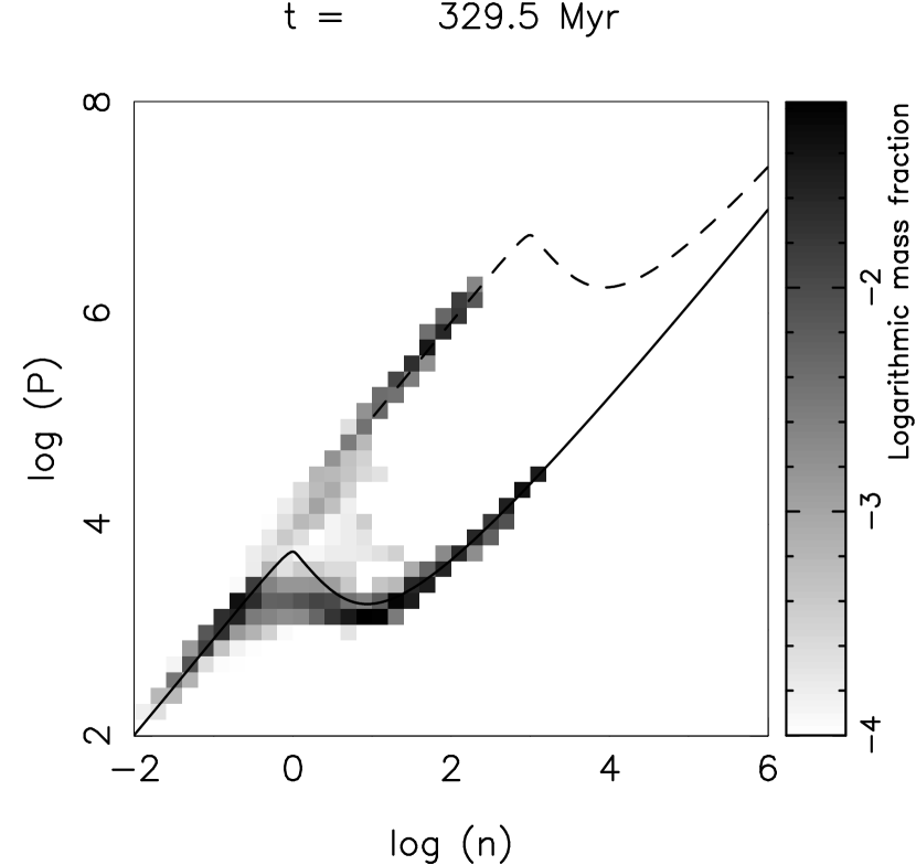
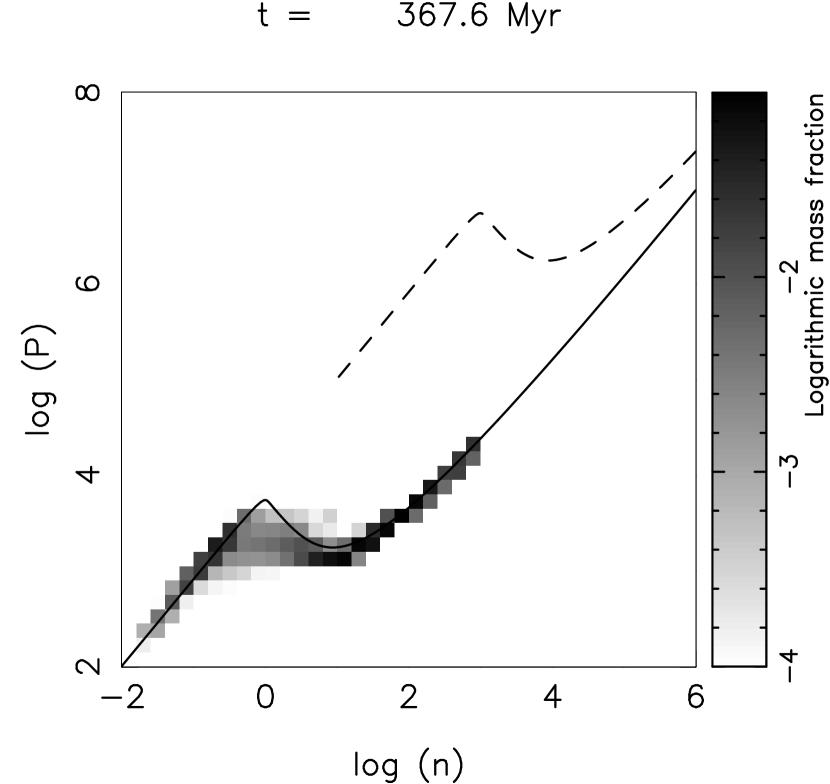
Figure 3: Phase diagram for Model Q11 snapshots shown in Figures 1 and 2. The gray scale shows the relative fraction of the total mass at each point in the phase plane. The solid line denotes the thermal equilibrium curve at the background heating rate ($G_{\rm FUV}=1$); the dashed curve shows thermal equilibrium in HII regions ($G_{\rm FUV}=10^{3}$). The snapshot from Figure 1 is taken while an HII region is very young, and there is considerable gas on the hot, high-density branch; there is very little gas on the HII region branch from the second snapshot. Overall, gas is preferentially – but not exclusively – found near the thermal equilibrium curves.

To allow for multiphase interstellar gas components, we must solve a thermal energy equation that allows a wide range of conditions. We use a cooling function for the diffuse ISM derived by Koyama & Inutsuka (2002), which includes atomic gas cooling for the warm and cold neutral medium (WNM, CNM), as well as cold molecular-phase cooling (H₂, CO, and dust cooling). We include a constant volumetric heating rate to represent photoelectric heating by diffuse FUV. This yields a standard (cf. Field et al. 1969; Wolfire et al. 1995) thermal equilibrium curve in which there is a maximum density and pressure for the warm phase given by $1.0~{}{\rm cm}^{-3}$ and $5.5\times 10^{3}~{}k_{\rm B}~{}{\rm cm}^{-3}{\rm K}$, and a minimum density and pressure for the cold phase given by $8.7~{}{\rm cm}^{-3}$ and $1.75\times 10^{3}~{}k_{\rm B}~{}{\rm cm}^{-3}{\rm K}$ (see Fig. 3).

HII regions in the real ISM include photoionization of atoms and dissociation of molecules, and radiative cooling of photoionized gas and warm molecular gas. These effects depend on chemical fractions, as well as dust evaporation. For this work, we are interested primarily in dynamics of the neutral media, rather than the details of photoionized gas – including the complexities of ionization front propagation at sub-parsec scales. The main requirement for capturing the large-scale dynamical effects of feedback is thus to incorporate photoheating of gas in star-forming regions. The simple but expedient approach we have chosen is to expose gas in targeted regions to enhanced heating, while simply applying the same cooling function we use for neutral gas. The enhanced heating we apply yields thermal equilibrium for the “photoheated” gas at $\approx 10,000$K (see below), which is consistent with the temperatures that would be attained if we had implemented realistic (but much more computationally complex and expensive) photoprocesses.

Cooling and heating timescales often become much shorter than the hydrodynamic time step (i.e. the flow or sound crossing time of a grid zone), especially in HII regions, which have a high heating rate. For efficiency, we adopt implicit time integration for the heating and cooling operators. In a given zone, the integral from the (j) to the (j+1) time step is formally expressed as

$$\int_{T_{j}}^{T_{j+1}}\frac{C_{v}dT}{\Gamma_{j}-n\Lambda(T)}=\Delta t_{j},$$ (20)

where $C_{v}=k_{\rm B}/(\gamma-1)$ is the heat capacity per particle. This is a nonlinear equation with respect to $T_{j+1}$, with $T_{j}$ and $\Delta t_{j}$ treated as parameters. For this integral, we adopt Simpson’s rule and solve using the Newton-Raphson method.

2.5 Thermal Conduction

Thermal conduction determines the thickness of interfaces between phases in the ISM, and proper incorporation of conduction is essential in numerical simulations of a multiphase medium which is subject to thermal instability (Piontek & Ostriker, 2004; Koyama & Inutsuka, 2004; Kim et al., 2008). The characteristic length scale set by conduction is the Field length,

$$\lambda_{\rm F}=2\pi\sqrt{\frac{KT}{n^{2}\Lambda(T)}},$$ (21)

(Field, 1965; Begelman & McKee, 1990), which corresponds to the critical wavelength of thermal instability. For realistic values of the conductivity at $T\ {\raise-2.15277pt\hbox{$\buildrel<\over{\sim}$}}\ 10^{4}{\rm K}$, $K=2.5\times 10^{3}\sqrt{T}$ erg cm^-1 s^-1 K^-1 (Parker, 1953), the Field length of 0.19 pc (at density $1~{}{\rm cm}^{-3}$ and temperature 1,000 K) is much smaller than the size of interstellar clouds ($\sim$ 1 – 10 pc) and we would need extremely high spatial resolution to resolve it – and a correspondingly high computational cost. Instead, we adopt an approach somewhat analogous to the use of artificial viscosity (far exceeding the true physical viscosity in magnitude) in resolving shocks on a numerical grid. Namely, we adopt a sufficiently large numerical conduction coefficient to resolve the Field length on our chosen grid. We choose $K$ such that for any simulation with resolution $\Delta x$, the Field number $N_{\rm F}\equiv\lambda_{\rm F}/\Delta x$ is equal to 1.7 at density and temperature typical of thermally unstable gas (we use $n=1\ {\rm cm}^{-3}$, $T=1,000$ K). For example, the fiducial model Q11 has $\Delta x=1.5$ pc and the artificial conductivity gives $\lambda_{\rm F}=2.57$ pc for thermally unstable gas.

For low density gas, given our typical values of $K$ the thermal conduction term can become greater than cooling/heating terms. In order to limit the conduction in these regions, we adopt

$$\tilde{K} = \frac{K}{1+n_{\rm crit}/n},$$ (22)

with $n_{\rm crit}=0.05~{}{\rm cm}^{-3}$.

2.6 Stellar Feedback Activity

The primary focus of this work is to explore the dynamical effects of strong, localized heating by OB stars in dense regions of the ISM. Since this heating produces $T\sim 10^{4}$ K gas that is initially overpressured by a factor $\sim 100$ or more compared to its surroundings, HII regions expand rapidly. This process is believed to be an important source of turbulence both within self-gravitating GMCs and in the surrounding diffuse ISM. To study this process, ideally one would implement (a) formation of OB stars from dense gas, distributed throughout the space-time domain of the simulation; (b) radiative transfer of ionizing photons from the OB stars through the surrounding gas, with potentially multiple ionization sources throughout the domain; (c) detailed ionization and heating of the gas within HII regions.

In this first exploration, rather than attempting to model all of these processes in an exact fashion, we instead adopt an idealized approach, with the goal of gaining physical understanding. First, we apply certain criteria to determine when and where “star zones” on the grid will be turned on. Then, we apply strong heating to the gas in the vicinity of each “star zone” for the duration of its lifetime. All “star zones” have the same lifetime, $t_{\rm ms}$, which is set to $3.7\times 10^{6}$ yr, the typical lifetime of OB associations in clouds whose mass is $10^{5}{\rm M}_{\odot}\$ (McKee & Williams, 1997). Within HII regions, we assume a constant gas heating rate, set via a control parameter $G_{\rm HII}$. Each “star zone” is therefore essentially a control flag for whether or not strong photoheating is locally applied near that zone (which does not move). Rather than solving a radiative transfer problem, we use a simple criterion based on the gravitational potential to determine whether gas is subject to strong heating. Because our goal is to identify gas localized around star-forming regions, it is necessary to subtract out the background gravitational potential and retain just the potential component due to an individual self-gravitating cloud.

The background potential is the potential averaged over horizontal planes. In terms of Fourier components, the relative gravitational potential $\Phi^{(1)}=\Phi-\Phi_{\rm background}$ is defined as

$$\Phi^{(1)}({\bf x})=\sum_{k_{z}\neq 0}\hat{\Phi}_{k}\hat{f}_{\bf k}\exp(-i{\bf k\cdot x}).$$ (23)

Here, $\hat{f}_{\bf k}$ is the Fourier component of a smoothing window function,

$$f({\bf x})=\frac{3}{4\pi r_{0}^{3}}\frac{1}{1+\exp\left[\frac{10}{\Delta x}(\sqrt{x^{2}+z^{2}}-r_{0})\right]},$$ (24)

where $r_{0}$ is a smoothing length. This window function smooths the HII region within a radius $\approx r_{0}$. Convolution of the relative potential with a smoothing function (or, equivalently, multiplication in Fourier space as above) is desirable so that any heating that is applied is resolved on the grid. We have adopted $r_{0}=3\Delta x$ as providing adequate resolution.

HII photoheated regions are identified as regions where the relative potential, $\Phi^{(1)}$, falls below some specified level: $\Phi^{(1)}<\Phi_{\rm HII}$. We also employ the relative potential $\Phi^{(1)}$ for setting one of the criteria for turning on feedback: $\Phi^{(1)}<\Phi_{\rm SF}$ and $\rho>\rho_{\rm SF}$ must both be met in a given zone for a “star zone” to be created at that location. Thus, our recipe ensures that feedback will only occur in dense and self-gravitating regions, consistent with the fact that OB stars are observed to form only under these conditions.

For the feedback prescription we have adopted, there are five control parameters: $\rho_{\rm SF}$, $\Phi_{\rm SF}$, $t_{\rm ms}$, $\Phi_{\rm HII}$, $G_{\rm HII}$. The detailed estimation of those parameters is described in the remainder of this section.

2.6.1 OB Star Formation Criterion

We choose a density threshold for star formation as

$$\rho_{\rm SF} = 10^{3}\mu\,{\rm cm}^{-3}.$$ (25)

This density is comparable to that of clumps of gas within GMCs. The free fall time at this density, 1.4 Myr, is sufficiently small compared to the orbital time that structures satisfying this threshold evolve independently of the global environment. Note that the local Jeans length

$$\lambda_{\rm J}=\left(\frac{\pi c_{s}^{2}}{G\rho_{\rm SF}}\right)^{1/2}=4.1\,{\rm pc}\left(\frac{c_{s}}{0.9~{}{\rm km\ s^{-1}}}\right)$$ (26)

must be resolved by a few zones in order to prevent fragmentation occurring as a consequence of numerical artifacts (Truelove et al., 1997).

To obtain an estimate for the potential threshold for star formation, we consider a cloud with uniform number density $\bar{n}$ and radius $R_{\rm cl}$. For a spherical cloud, the radius is related to the cloud mass using

$$R_{\rm cl} = \left(\frac{3M_{\rm cl}}{4\pi\bar{\rho}}\right)^{1/3}=19~{}{\rm pc}\times\bar{n}_{2}^{-1/3}M_{\rm cl,5}^{2/3},$$ (27)

where the fiducial value of $\bar{n}_{2}\equiv\bar{n}/(10^{2}~{}{\rm cm}^{-3})$ is chosen using a typical mean density within GMCs, and $M_{\rm cl,5}\equiv M_{\rm cl}/(10^{5}~{}{\rm M}_{\odot}\ )$.

Since our grid is two-dimensional, the control parameter $\Phi_{\rm SF}$ must be based on a cylindrical regions of a given density. For a cylinder of radius $R_{\rm cl}$, the potential difference between the center and a distance $r$ ($>R_{\rm cl}$) is $\Phi(0)=\Phi(r)-2\pi G\bar{\rho}R_{\rm cl}^{2}[\ln(r/R_{\rm cl})+1/2]$. The logarithmic term corresponds to the potential difference between $r$ and $R_{\rm cl}$, and the $1/2$ is the contribution between the cloud’s surface and its center. If the cloud is created out of all of the mass originally within a disk of surface density $\Sigma$ within a range $2r\equiv L_{\rm eqv}$ of the cloud center, then $\pi R_{\rm cl}^{2}\bar{\rho}=\Sigma L_{\rm eqv}$, and a fiducial distance for defining the effective zero of the potential is

$$L_{\rm eqv} = \frac{\pi\bar{\rho}R_{\rm cl}^{2}}{\Sigma},$$ (28)

$$= 393~{}{\rm pc}\times\bar{n}_{2}M_{\rm cl,5}^{2/3}\left(\frac{\Sigma}{10{\rm M}_{\odot}\ {\rm pc}^{-2}}\right)^{-1}.$$ (29)

Here, the radius is expressed in terms of that of an equivalent spherical cloud with a given mass. If we set the potential at $r=L_{\rm eqv}/2$ to zero, then the potential at the center of the cloud will be

$$\Phi(0)=-\Phi_{\rm SF}\equiv-2\pi G\bar{\rho}R_{\rm cl}^{2}\left[\ln\left(\frac{L_{\rm eqv}}{2R_{\rm cl}}\right)+\frac{1}{2}\right].$$ (30)

For $\bar{n}=100~{}{\rm cm}^{-3}$ and $R_{\rm cl}=19$ pc, the value of $\Phi(0)$ is $3.4\times 10^{11}{\rm cm}^{2}~{}{\rm s}^{-2}$ times an order-unity factor that varies only logarithmically in the ratio of cloud surface density to mean ISM surface density. We choose to adopt a potential threshold for star formation $\Phi_{\rm SF}=3.4\times 10^{11}{\rm cm}^{2}~{}{\rm s}^{-2}=(5.8{\rm km}~{}{\rm s}^{-1})^{2}$; we have tested sensitivity to the value of $\Phi_{\rm SF}$, and found that results are insensitive to the exact choice, except as described below.

2.6.2 Definition of Photoheated Regions

First, consider an HII region centered on the origin of a uniform cloud with spherical crossection. If we assume the radius of the HII region is $R_{\rm HII}$ ($<R_{\rm cl}$), then if the center of the cloud has potential $\Phi(0)$, the potential at the ionization front for a cylindrical cloud with uniform density is $\Phi_{\rm HII}=\Phi(0)+\pi G\bar{\rho}R_{\rm HII}^{2}$. (For a spherical cloud, the second term is smaller by a factor $2/3$.) Taking the difference with $\Phi(L_{\rm eqv}/2)$ in order to represent a relative potential, using equation (30), and substituting $\Phi(0)\rightarrow-\Phi_{\rm SF}$ (since the criterion for star formation must be satisfied if feedback has turned on) this implies that the relative potential at the location of the HII region would be

$$\Phi_{\rm HII}=-\Phi_{\rm SF}\left[1-\frac{\frac{1}{2}}{\ln\left(\frac{L_{\rm eqv}}{2R_{\rm cl}}\right)+\frac{1}{2}}\left(\frac{R_{\rm HII}}{R_{\rm cl}}\right)^{2}\right].$$ (31)

$R_{\rm HII}$ is given, for example, by the Strömgren radius in a uniform medium:

$$R_{\rm HII} = \left(\frac{3S}{4\pi\bar{n}^{2}\alpha^{(2)}}\right)^{1/3}=2.97~{}{\rm pc}~{}\bar{n}_{2}^{-2/3}S_{49}^{1/3},$$ (32)

where $S$ is the number ionizing photons per unit time and $S_{49}\equiv S/(10^{49}{\rm s}^{-1})$, and $\alpha^{(2)}=3.09\times 10^{-13}~{}{\rm cm}^{3}{\rm s}^{-1}$ is the case B hydrogen recombination coefficient at $T=8,000$ K (Spitzer, 1978). $S_{49}$ is equal to unity for the ionizing luminosity in a typical $10^{5}{\rm M}_{\odot}\$ GMC (McKee & Williams, 1997). From equation (31), when the density is comparable to the mean density within a GMC, $R_{\rm HII}/R_{\rm cl}\ll 1$, and the HII region is buried deep within the GMC at $||\Phi_{\rm HII}|-\Phi_{\rm SF}|/\Phi_{\rm SF}\ll 1$.

HII regions are initially highly overpressured, however, and will expand rapidly until breaking out of the surrounding GMC, creating a blister HII region. For the purposes of considering the momentum input to the system, the $R_{\rm HII}\rightarrow R_{\rm cl}$ limit is most appropriate for defining the photoheated region. Thus, we suppose that the HII region has expanded, leaving a very low density interior and a shell of radius $R_{\rm HII}<R_{\rm cl}$ in which most of the mass has piled up. The potential in the interior of the shell is then given by

$$\Phi_{\rm HII}=-\Phi_{\rm SF}\left[1-\frac{\frac{R_{\rm HII}^{2}}{R_{\rm cl}^{2}-R_{\rm HII}^{2}}\ln(\frac{R_{\rm cl}}{R_{\rm HII}})}{\ln\left(\frac{L_{\rm eqv}}{2R_{\rm cl}}\right)+\frac{1}{2}}\right].$$ (33)

When $R_{\rm HII}\rightarrow R_{\rm cl}$, this expression is of course the same as if we had taken $R_{\rm HII}/R_{\rm cl}\rightarrow 1$ in equation (31), that is, the potential near the surface of the initially-uniform cloud. For convenience, we introduce a dimensionless parameter $\epsilon$:

$$\Phi_{\rm HII}\equiv-\Phi_{\rm SF}(1-\epsilon),$$ (34)

where $\epsilon=(1/2)[\ln\left(\frac{L_{\rm eqv}}{2R_{\rm cl}}\right)+\frac{1}{2}]^{-1}$ when $R_{\rm HII}\rightarrow R_{\rm cl}$. For the fiducial parameter values discussed above, $\epsilon$ is equal to 0.18. We therefore adopt $\epsilon=0.2$ as our “standard” value, although we have tested how the results differ for much smaller values.

2.6.3 Heating Rate in HII Regions

During the period that “star zones” are alive, UV photons enhance the heating rate within HII regions, defined as described above. For the heating rate in any zone due to UV photons, we adopt the on-the-spot approximation given by:

$$\Gamma = 2.16\times 10^{-26}G_{\rm FUV}~{}{\rm erg}~{}{\rm cm}^{-3}{\rm s}^{-1},$$ (35)

$$G_{\rm FUV} = \left\{\begin{array}[]{ll}G_{\rm HII}&\mbox{($\Phi^{(1)}<\Phi_{\rm HII}$)},\\ G_{0}&\mbox{(otherwise)},\\ \end{array}\right.$$ (38)

where $G_{0}=1.0$ is the background FUV field in the Galaxy.

We choose $G_{\rm HII}=10^{3}$ throughout this paper, although we have also tested results with lower and higher $G_{\rm HII}$. In practice, the exact value of $G_{\rm HII}$ is not important, since the purpose of this added heating is simply to increase the maximum density at which a warm phase is present. From our Fig. 3 (see also e.g. Fig. 7 of Wolfire et al. 1995), a value of $G_{\rm HII}=10^{3}$ boosts this to $n\sim 10^{3}~{}{\rm cm}^{-3}$.

3 Model Parameters

The models in this paper are characterized by three main parameters: the total gas surface density $\Sigma$, the orbital angular velocity $\Omega$ in the center of the domain, and the stellar density at the midplane $\rho_{\ast}$. The first parameter defines the amount of raw material available for distribution between the dense and diffuse ISM phases, while the second two parameters define the galactic environment in which the gas evolves in response to the galactic tidal, rotational, and shear stresses. The effectiveness of self-gravity in forming massive clouds depends on all of these parameters, as well as on the turbulent state that develops as a consequence of star formation feedback.

The simulation domain we model is a radial-vertical slice through a disk. For the vertical direction, we require a domain $L_{z}$ that encloses most of the mass of the ISM, which is confined by a combination of stellar gravity and gas self-gravity. The largest scale height (excluding the hot ISM, absent in these models) is that of the WNM, and an upper limit is obtained by neglecting self-gravity, which yields a Gaussian distribution with scale height:

$$H_{w} = \frac{c_{w}}{\sqrt{4\pi G\rho_{\ast}}}=95~{}{\rm pc}\left(\frac{c_{w}}{7~{}{\rm km\ s^{-1}}}\right)\left(\frac{\rho_{\ast}}{0.1~{}{\rm M}_{\odot}\ {\rm pc}^{-3}}\right)^{-1/2}.$$ (39)

Here, $c_{w}=(kT_{w}/\mu)^{1/2}$ is the thermal speed of the warm medium, which typically has $T_{w}=8,000-10,000$ K. We require $L_{z}>2H_{w}$ for our numerical models.

If the ISM consisted only of WNM, then with $n_{w,0}=\rho_{w,0}/\mu$ the central volume density, the total surface density would be

$$\Sigma_{w}=\sqrt{2\pi}\rho_{w,0}H_{w}=1.6~{}{\rm M}_{\odot}\ {\rm pc}^{-2}\left(\frac{n_{w}}{0.2~{}{\rm cm}^{-3}}\right)\left(\frac{c_{w}}{7~{}{\rm km\ s^{-1}}}\right)\left(\frac{\rho_{\ast}}{0.1~{}{\rm M}_{\odot}\ {\rm pc}^{-3}}\right)^{-1/2}.$$ (40)

The maximum density for which the warm phase is possible (when $G_{0}=1$) is $n_{w,{\rm max}}=P_{w,{\rm max}}/(\mu c_{w}^{2})\approx 1~{}{\rm cm}^{-3}$; this implies a maximum possible total surface density of warm gas $\Sigma_{w,{\rm max}}=(2G\rho_{\ast})^{-1/2}P_{w,{\rm max}}/c_{w}$. In practice, the midplane density of the warm medium is closer to the value $0.23~{}{\rm cm}^{-3}$, which represents the warm medium density that is in pressure equilibrium with cold gas at $P_{c,{\rm min}}/k_{\rm B}=1.75\times 10^{3}{\rm cm}^{-3}{\rm K}$. We are interested in multiphase disks similar to those observed in the Solar neighborhood and at smaller radii in normal spirals; hence we choose surface density of at least several ${\rm M}_{\odot}\ {\rm pc}^{-2}$ such that the pressure is high enough to permit a cold phase to form, i.e. $\Sigma>(2G\rho_{\ast})^{-1/2}P_{c,{\rm min}}/c_{w}$.

The radial domain should be sufficient to capture the largest-scale gravitational instabilities, which in a disk galaxy are limited by angular momentum. The Toomre length (Toomre, 1964) is the maximum scale for axisymmetric modes in a thin, cold disk;

$$\lambda_{T} = \frac{4\pi^{2}G\Sigma}{\kappa^{2}}=\frac{4\pi^{2}G\Sigma}{(4-2q)\Omega^{2}},$$ (41)

$$= 1.36~{}{\rm kpc}\left(\frac{\Omega}{25~{}{{\rm km\ s^{-1}}~{}{\rm kpc}^{-1}}}\right)^{-2}\left(\frac{\Sigma}{10~{}{\rm M}_{\odot}\ /{\rm pc}^{2}}\right).$$ (42)

We require $L_{x}>\lambda_{T}$ for our numerical models, typically by a factor 1.3.

The parameters of our models are summarized in Table 1. In order to cover the three-dimensional parameter space and explore environmental dependences systematically, we consider four series of models: Q, K, S, and R. For each Series, we hold two quantities fixed and vary a third quantity, as follows:

• Series Q: $\kappa/\Sigma$ and $\sqrt{\rho_{\ast}}/\Sigma$ are constant while $\Sigma$ varies;

• Series K: $\kappa$ and $\sqrt{\rho_{\ast}}/\Sigma$ are constant while $\Sigma$ varies;

• Series R: $\kappa/\Sigma$ and $\rho_{\ast}$ are constant while $\Sigma$ varies;

• Series S: $\Sigma$ and $\rho_{\ast}$ are constant while $\kappa$ (and $\Omega$) varies.

The value of the Toomre $Q$ parameter for the gas component, for a radial velocity dispersion $\sigma_{R}$, is defined as

$$Q \equiv \frac{\kappa\sigma_{R}}{\pi G\Sigma}$$ (43)

$$= 1.82\left(\frac{\Omega}{25{\rm km~{}s^{-1}~{}kpc^{-1}}}\right)\left(\frac{\sigma_{R}}{7\,{\rm km~{}s^{-1}}}\right)\left(\frac{\Sigma}{10{\rm M}_{\odot}\ {\rm pc}^{-2}}\right)^{-1}.$$ (44)

Since Toomre’s parameter is proportional to $\kappa/\Sigma$, Series Q and R would have constant thermal $Q=\kappa c_{s}/(\pi G\Sigma)$ for the gas if the sound speed $c_{s}$ were constant (which is true for warm gas). The Q and R series correspond to values of $Q=2.1(\sigma_{R}/7~{}{\rm km\ s^{-1}})$. Assuming a constant stellar velocity dispersion, $\Sigma_{\ast}\propto\sqrt{\rho_{\ast}}$, so the stellar Toomre parameter ($Q_{\ast}\propto\kappa/\Sigma_{\ast}$) would also have the same value for all members of Series Q. As a fiducial model, we choose $\Sigma=10.6~{}{\rm M}_{\odot}\ /{\rm pc}^{2}$, $\Omega=31.2~{}{\rm km\ s^{-1}}~{}{\rm kpc}^{-1}$, and $\rho_{\ast}=0.07~{}{\rm M}_{\odot}\ /{\rm pc}^{3}$, similar to conditions in the Solar neighborhood; this is denoted as the Q11 model in Table 1.

Relative to conditions similar to those in the Solar neighborhood, we may think of the members of Series Q as representing conditions ranging from slightly larger radii down to radii of a few kpc, for a disk that has constant $Q$ and $Q_{\ast}$ – i.e. larger gas and stellar densities at small radii. We may think of Series R as models spanning a similar range of radii, except for a disk that has stellar density (and the corresponding vertical gravity) independent of radius, while the gas surface density increases inward (such that the gas self-gravity can become dominant). We may think of Series S as relocation of the Solar neighborhood conditions of gas and stellar density to either further in or further out in the galaxy’s potential well, where rotation and shear are stronger or weaker, respectively. We may think of Series K as choosing a fixed location in the galactic potential well (dominated by dark matter), and then varying the gas and stellar surface densities in tandem.

To initialize our models, we set the density to a uniform value (given by $\bar{n}$ in Table 1) throughout the domain, and set the pressure to $P/k_{\rm B}=4,860~{}{\rm cm}^{-3}{\rm K}$ which is in the thermally unstable regime. The value of the initial pressure in fact does not matter, since the gas rapidly separates into WNM and CNM due to thermal instability. We also impose on the initial conditions isobaric density perturbations (with a flat spectrum at wavenumbers smaller than $kL_{z}/2\pi=32$, and 10 % total amplitude). The results are also not sensitive to the amplitude or power spectrum of the initial perturbation spectrum; this is simply a convenience to seed the initial evolution into thermal instability and then Jeans fragmentation of cold gas. In order to reach a quasi-steady state with repeated feedback cycles, we run our models for two orbital periods in Series Q, R and K and up to $t_{\rm final}=5.57\times 10^{8}$ year for Series S.

3.1 Hydrostatic Models

Because an important focus of this work is to assess the effects of turbulence, it is important to ascertain how our dynamical models differ from the situation in which there are no motions other than background sheared rotation. For these comparison models, we calculate the one-dimensional hydrostatic equilibria in the vertical direction. These models include heating and cooling, but no feedback from star formation. We consider two series, HSP and HSC which have stellar volume density $\rho_{*}$ either proportional (P) to the square of the gas surface density $\Sigma$ or constant (C), respectively. Note that Series HSP corresponds to the dynamical Series Q and K, while Series HSC corresponds to the dynamical Series R. Details of these model parameters are listed in Table 2. Uniform 1024 grids are used for all hydrostatic models. Note that the hydrostatic models only allow one-dimensional vertical structure, and require higher spatial resolution than the dynamic models because the scale height in the cold layer near the midplane becomes very small when there is no feedback.

4 Evolution of the Fiducial Model

This section describes the overall evolution of the fiducial model. After the initial thermal instability, the cold gas collapses into the midplane, due to the vertical gravitational field. The cold, high-density midplane gas then fragments rapidly, due to self-gravity. The time scale for this fragmentation is characterized by the Jeans time for a thin disk, $t_{\rm J}=c_{s}/G\Sigma\approx 6~{}{\rm Myr}(c_{s}/0.3~{}{\rm km~{}s^{-1}})$. The dense fragments collapse, with some of them coagulating, until the feedback criteria are met, and heating is turned on to create local HII regions. These HII regions expand, causing the dense gas to be swept outward, forming shells that then break up into filaments. New overdense regions continue to form, collapse, and be dispersed by feedback.

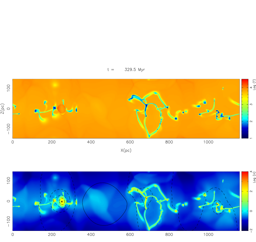
Figure 1: A snapshot of Model Q11, with $\Sigma=10.6{\rm M}_{\odot}\ {\rm pc}^{-2}$: Upper panel shows temperature, and Lower panel shows density; both have logarithmic color scales as shown. Contours in the lower panel are loci of constant $\Phi^{(1)}$, the relative potential, with solid and dashed curves for $\Phi^{(1)}>0$ and $\Phi^{(1)}<0$, respectively. The black asterisk at the potential minimum in the left part of the panel indicates the location of a “star zone” feedback center. The cold, dense gas is highly clumpy and filamentary, and is concentrated toward the midplane by self- and external gravity.

Figure 1 shows a snapshot from the fiducial model (Model Q11) at a point after the system has reached a quasi-steady state, in terms of the statistical distributions of density, temperature, and velocity. The two panels show the temperature and density throughout the domain. The contours in the lower panel denote relative potential $\Phi^{(1)}$: solid and dashed lines show positive and negative values, respectively. At the time of this snapshot, there are three large clouds consisting of collections of dense filaments that create minima in the gravitational potential (dashed lines in the lower panel). Most of the dense filaments and clumps in the lower panel correspond to cold gas in the upper panel. In the upper panel, the orange circle associated with the cloud near $x=250$ pc shows an active HII region, in which the gas is both warm and dense and hence is expanding rapidly. Expansion of shells slows at later times (after the pressure drops to ambient values and the enhanced heating turns off). Since most of the time for any given shell is spent near the maximum expansion, the widely-expanded structure of the middle cloud is typical, in terms of the time-averaged state.

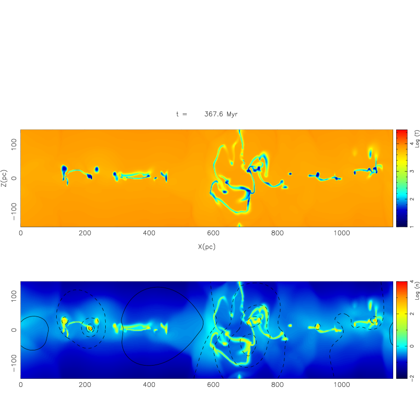
Figure 2: A later-time ($\Delta t$= 38 Myr) snapshot of temperature (top) and density (bottom) from Model Q11, showing that individual structures have dynamically evolved. See Figure 1 legend for details.

Figure 2 shows a snapshot of the density and temperature in the same model Q11 at a time 38 Myr later. Overall, the structure is qualitatively similar, although details change because the state is highly dynamic. There are still three main collections of filaments; the middle cloud has a large shell while the left- and right-side clouds have contracted onto the midplane and have nearly reached the point at which new HII regions will be born.

Three large “clouds” within the 1.16 kpc horizontal length of the domain corresponds to mean separations of 390 pc. One might expect the number of cloud entities to be related to the properties of star formation feedback, and for our adopted prescription to the parameter $\epsilon$, which effectively determines the maximum volume of an HII region: large $\epsilon$ corresponds to large HII regions, whereas small $\epsilon$ corresponds to HII regions only in the immediate vicinity of a potential minimum defined by a high-density clump of gas. In a situation with multiple local minima in the gravitational potential, if $\epsilon$ is large then a single HII region could engulf what would be multiple HII regions in the case of small $\epsilon$. Expansion and shell collision of many small HII regions would produce more (but smaller) clouds than expansion and collision of a few large HII regions. In fact, when we run the same model but set $\epsilon=0.02$, we find that there are typically 4-5 clouds in the same domain. We conclude that the number of large clouds is not very sensitive to $\epsilon$, but since this control parameter can only approximately model the effects of real HII regions, the current study cannot provide an exact prediction for the size or mass of GMCs. We note that the typical separation is, however, in the same range as the two-dimensional Jeans length at the typical velocity dispersion, $\lambda_{\rm J,2D}\equiv\sigma^{2}/(G\Sigma)=340{\rm pc}(\sigma/4~{}{\rm km~{}s^{-1}})^{2}$ for this model.

Figure 3 shows the phase diagram ($\rho-P$ plane) for the same snapshot in Figure 1 and 2. The gray scale is proportional to the fraction of the total mass in the domain that is found at a given point in the phase plane. We overlay the thermal equilibrium curves for both the cases of “normal” heating (solid curve) and the enhanced heating in HII regions (dashed curve). Clearly, most of the gas resides near thermal equilibrium, due to the short cooling times compared to the longer hydrodynamical times.

The range of properties of the gas can also be seen in the Figure 4, which shows the probability distribution functions (PDFs) of gas density. Solid and dashed lines show mass and volume weighted probabilities, respectively. The volume PDF shows that the volume is mainly occupied by warm and diffuse gas (WNM) at densities of a few $\times 0.1~{}{\rm cm}^{-3}$. In terms of the mass PDF, there are two peaks: one corresponds to the WNM, and the other to a cold component at density above $10~{}{\rm cm}^{-3}$.

Figure 5 shows the time evolution of thermal, kinetic and potential energies averaged over the domain, for Model Q11. For the potential energy, the background disk potential is subtracted out; i.e. we use $\Phi^{(1)}$ (see eq. 23). There are many sharp spikes in both thermal and kinetic energies, which correspond to times when new HII regions are born and then rapidly expand. The number of spikes corresponds to the number of stellar generations in the model; note that this number must be proportional to the domain size. In the second rotational period (i.e., $1\leq t\leq 2$ rotation), there are 18 generations per 1.16 kpc, or 6 generations per massive cloud per rotation period (i.e. an interval of $3.3\times 10^{7}$ yr) if the mean number of clouds is 3 in this fiducial model.

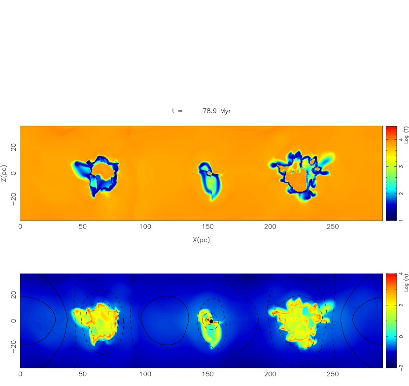
Figure 6: A snapshot of temperature (top) and density (bottom) in high surface density Model Q42. See Figure 1 legend for details.

Other models show similar overall behavior in terms of the evolution of physical structure (consisting of clumps and filaments that disperse and re-collect), as well as the distribution of mass in the phase plane. As environmental parameters vary along a sequence, however, there are some characteristic changes in structure. The most notable difference is that for high gaseous surface density cases, clouds are often more physically concentrated (i.e., more compact and dense) because of the higher stellar and gaseous gravity. For example, Figure 6 shows a snapshot from Model Q42, which has $\Sigma$ and $\rho_{\ast}$ four and 16 times larger, respectively, than the values in the fiducial model Q11. The three clouds that are seen in the figure are more compact than in the lower-$\rho_{\ast}$ case. For a given $\Phi_{\rm SF}$ and $\epsilon$, increasing the mass of a cloud implies that HII region cannot break out as easily.

5 Parameter Dependence of Statistical Properties

All of our models show a turbulent, multiphase ISM with several generations of feedback from photoheating. In this section, we analyze how the statistical properties of those models depend on the environmental parameters, both along a given series and from one series to another. The statistical properties that we study are based on averages of the fluid variables over space and time. First we describe how these averages are defined in general, and then we turn to the particular statistics.

5.1 Space and Time Averaging Procedure

For a variable of $A$ that is averaged over both space and time, we use mass-weighted averages defined by:

$$\langle A(a)\rangle \equiv \frac{\int_{a}A\,dm}{M(a)},$$ (45)

$$M(a) \equiv \int_{a}\,dm,$$ (46)

where the argument ‘$a$’ denotes a given phase or component of the gas (such as WNM). The time averaging is then defined via:

$$\overline{\langle A(a)\rangle} \equiv \int_{t_{1}}^{t_{2}}\langle A(a)\rangle\,dt\Big{/}S,$$ (47)

$$S \equiv \int_{t_{1}}^{t_{2}}\theta(M(a))dt,$$ (48)

where the step function $\theta$ gives $1$ if $M(a)>0$ and $\theta=0$ otherwise, so that only intervals in which the component is present are included in the averaging. Note that $S=t_{2}-t_{1}$ if the component ‘$a$’ is present somewhere in the domain at every interval during the simulation. Thus, we denote spatial and temporal averages using angle brackets and overlines, respectively. To avoid the initial transients at the beginning of the simulation, we adopt the interval between $t_{1}=t_{\rm final}/2$ and $t_{2}=t_{\rm final}$ for our time average. For the purpose of averaging, our sampling rate is $\Delta t=0.1t_{\rm ms}$, where $t_{\rm ms}=3.7\times 10^{6}$ yr is the adopted lifetime of “star zone” flags that control photoheating feedback.

5.2 Mass Fractions

The models of this paper focus on dynamics rather than chemistry, so rather than dividing the gas into distinct phases, we simply bin it according to density. The neutral gas (i.e. the gas that is not within the limits defining HII regions) is separated into four bins. The first bin ($n<1~{}{\rm cm}^{-3}$) corresponds approximately to the WNM, with densities below the maximum for which a warm phase is possible in thermal equilibrium. The second bin ($1~{}{\rm cm}^{-3}<n\leq 100~{}{\rm cm}^{-3}$) extends up to the maximum density that is in pressure equilibrium with WNM gas, and corresponds approximately to the CNM (phase diagrams show that the thermally-unstable regime is not highly populated for our models; see e.g. Figs 3 and 4). The dense medium (hereafter DM) is all the gas at $n\geq 100~{}{\rm cm}^{-3}$, which in thermal equilibrium is above the maximum pressure for the warm phase and therefore only exists in regions that are internally stratified due to gravity. The DM gas corresponds approximately to the molecular component of the ISM; we divide it into two bins, DM2 ($100<n\leq 10^{3}$) and DM3 ($10^{3}<n$). Gas that is within the limits defined for enhanced heating is labeled as ionized gas (hereafter HII). So that the mass fractions $f(a)$ of all components add to unity, $\sum_{a}f(a)=1$, we use a slightly different definition from that of equation (47). The mass fraction of each component $a$ in (WNM, CNM, DM2, DM3 or HII) is defined as

$$f(a)=\frac{\displaystyle\int_{t_{1}}^{t_{2}}\frac{M(a)}{M_{\rm tot}}\,dt}{t_{2}-t_{1}}.$$ (49)

Figure 7 shows the mass fraction of the various components either as a function of surface density (Series Q, R and K) or angular velocity (Series S). For Series Q and R (which most closely correspond to the radial variations found within normal spiral galaxies), at low $\Sigma$ the diffuse (WNM+CNM) components dominate, while at high $\Sigma$ the dense (gravitationally-confined) components (DM2+DM3) dominate. The behavior is somewhat different in Series K, which is highly gravitationally unstable and thus extremely active when $\Sigma$ is large (since $\kappa$ is constant), leading to larger HII and CNM mass fractions at high $\Sigma$. At low $\Sigma$, the behavior in Series K is similar to that in Series Q and R. For all series, the HII mass fraction increases at higher $\Sigma$ or lower $\Omega$, corresponding to lower Toomre $Q$ (see Figure 11) and hence higher rates of stellar feedback activity. The mass fraction of the WNM component secularly declines with increasing $\Sigma$ in model series Q, K, and R. Even though the models of Series S are most gravitationally unstable at low $\Omega$, they remain dominated by diffuse gas (CNM) rather than dense gas, because the total surface density is relatively modest for this series ($\Sigma=15~{}{\rm M}_{\odot}\ {\rm pc}^{-2}$).

5.3 Surface Density

The simulation domain for our two-dimensional models represents a radial-vertical ($x-z$) slice through a galactic disk, such that if we viewed the corresponding galaxy face-on, the surface density as a function of radius would be given by $\Sigma(x)=\int dz\rho(x,z)$. The area-weighted mean surface density in any model is equal to $\langle\Sigma\rangle_{A}\equiv\int dxdz\,\rho/L_{x}$; this is a conserved quantity for any simulation, and is one of the basic model parameters (see column 2 of Table 1; in general we omit the angle brackets and “A” subscript). The value of the surface density weighted by mass rather than by area better represents the “typical” surface density of clouds found in the disk. This is defined as

$$\Sigma_{\rm cloud}=\frac{\int\Sigma(x)^{2}\,dx}{\int\Sigma(x)\,dx}.$$ (50)

Figure 8 shows $\Sigma_{\rm cloud}$ as a function of $\Sigma$ for all model series. Interestingly, we find that $\Sigma_{\rm cloud}$ does not strongly depend on parameters (either $\Sigma$ or $\Omega$) throughout the four model series. The largest value of $\Sigma_{\rm cloud}$ is $300{\rm M}_{\odot}\ {\rm pc}^{-2}$ and the smallest is $50{\rm M}_{\odot}\ {\rm pc}^{-2}$, although for most cases the range is even smaller: $\Sigma_{\rm cloud}=70-150{\rm M}_{\odot}\ {\rm pc}^{-2}$. This factor-of-two range for $\Sigma_{\rm cloud}$ is significantly smaller than the factor-of-six range of mean surface densities, $\Sigma=7.5-42{\rm M}_{\odot}\ {\rm pc}^{-2}$. The range of $\Sigma_{\rm cloud}$ is also similar to the typical observed surface densities of giant molecular clouds (see discussion in §7).

This weak variation of $\Sigma_{\rm cloud}$ among the various series suggests that it is star formation feedback, rather than the feedback-independent parameters, that determines the typical surface density of clouds. In particular, other tests we have performed suggest that it is the gravitational potential threshold for star formation $\Phi_{\rm SF}$ that most influences $\Sigma_{\rm cloud}$. A model in which $\Phi_{\rm SF}\to 0$ (with any $\epsilon$) would have photoheating events independent of the local ISM properties; the consequent expansion of HII regions would thoroughly mix gas so that $\Sigma_{\rm cloud}\to\Sigma$. This is indeed what we find when we run models with $|\Phi_{\rm SF}|$ a factor 10 below our adopted value. On the other hand, larger values of $|\Phi_{\rm SF}|$ require more massive and compact clouds in order to have star formation, which would raise $\Sigma_{\rm cloud}$. Tests with $|\Phi_{\rm SF}|$ a factor 10 above our adopted value indeed result in larger $\Sigma_{\rm cloud}$ (although only by a factor $\sim 2$). The dependence on $\epsilon$ is much weaker than the dependence on $\Phi_{\rm SF}$; reducing $\epsilon$ by a factor 10 changes $\Sigma_{\rm cloud}$ by only tens of percent, at our standard $\Phi_{\rm SF}$.

The comparison between Series Q and Series R is also interesting, in this regard. The difference between these two series is that the stellar density $\rho_{\ast}$ increases with $\Sigma$ in Series Q, while $\rho_{\ast}$ is constant throughout Series R. Based on the larger $\Sigma_{\rm cloud}$ value for the largest $\Sigma$ in Series Q compared to Series R, when the stellar density is increased, the surface density required in order to form clouds also increases.

5.4 Temperatures

Figure 9 shows the space-time averages of temperature for the components we have defined via density bins, $\overline{\langle T(a)\rangle}$, where the argument ‘$a$’ denotes WNM, CNM, DM2, DM3 and HII. Throughout the model series, the temperatures for the most dense and most diffuse components are fairly constant; we find $T=6,000-7,000$ K for WNM, $T=20-40$ K for DM2, and $T=10-20$ K for DM3. For the CNM component (which in fact includes thermally-unstable gas when it exists), the range is somewhat larger, $T=100-400$ K, reflecting the larger range of conditions for this gas. The gas which is subject to enhanced heating has mean temperatures for most models of 4,000 – 8,000 K.

The link between density and temperature in our models implies that the components we have defined via density bins also approximately correspond to natural ISM phases. This is because much of the gas mass is close to thermal equilibrium (see Figure 3), and we have chosen the bin edges so as to match up to points in the phase plane with physical significance. Temperature PDFs that we have constructed show a bimodal distribution, as is expected based on the cooling function.

5.5 Turbulent Velocities

Expansion of HII regions feeds kinetic energy into the ISM. This kinetic energy is not imparted solely to expanding HII bubbles and shells surrounding them, but is shared throughout the ISM as turbulence. Our models provide a first look at the results of this form of turbulent driving. It is interesting to examine how the turbulent amplitudes vary from one component to another in a given model, and how the overall levels vary between models with different feedback rates as a consequence of different system parameters.

Figure 10 shows the turbulent velocity dispersions for all series, defined for each component as:

$$v(a) \equiv \sqrt{\overline{\langle v_{x}(a)^{2}+\tilde{v}_{y}(a)^{2}+v_{z}(a)^{2}\rangle}},$$ (51)

where the argument ‘$a$’ denotes WNM, CNM, DM2, DM3 and HII, and $\tilde{v}_{y}=v_{y}+\Omega x$ in order to subtract out the velocity of unperturbed (sheared) rotation about the galactic center. The azimuthal velocities are excited by Coriolis forces so that the relation for epicyclic motions

$$\frac{{\tilde{v}}_{y}}{{v}_{x}}\simeq\frac{\kappa}{2\Omega}=\frac{1}{\sqrt{2}}$$ (52)

should apply (Binney & Tremaine, 1987), and we have checked that this is in fact satisfied. We note that the velocity dispersion for each component is computed by summing over the whole domain. Thus, the measured velocity dispersions are larger than they would be within smaller-scale clouds in the system. However, we have found that there are not large contributions to the velocity dispersion from velocity differences of widely-separated regions; this is because turbulence is driven by the expanding HII regions, such that the maximum correlation scale is comparable to the effective thickness of the disk. For example, if we divide the domain in Fig. 1 horizontally into eight equal parts, the mean velocity dispersion of all gas within these sub-domains is $\sim 98\%$ of that of the domain as a whole. Considering just the dense gas, the velocity dispersion for subdomains is $\sim 75\%$ of that in dense gas for the whole domain. For the three large clouds seen in Fig. 6, the mean internal velocity dispersions are an order of magnitude larger than the dispersion in mean velocities.

In general, the densest component (DM3) has the lowest velocity dispersion, with the next-densest (DM2) the next-lowest. The value of the velocity dispersions for the dense components are highly supersonic, and are similar to (or slightly below) those that are observed within real GMCs (see §7). The CNM component in our models typically has higher turbulence levels than the WNM component, because the former is in closer (space-time) contact with energy sources. Because turbulent motions in our models are driven by the pressure of photoheated gas, $P=\rho c_{s}^{2}\sim\rho v^{2}$, the turbulent velocities have an upper limit of the sound speed in gas heated to 8,000 K, $c_{\rm HII}\sim 7~{}{\rm km\ s^{-1}}$. Since the driving is intermittent, this upper limit is not usually reached; mean values for the diffuse gas are closer to $\sim 5~{}{\rm km\ s^{-1}}$. The diffuse-gas velocity dispersions in our models are lower by about 50% compared to observed levels, indicating (consistent with expectations) that other turbulence sources are important in the real diffuse ISM.

The model series Q and R, which have $\Sigma\propto\Omega$ (and thus effectively constant gaseous Toomre $Q$ if the velocity dispersion is constant) show velocity dispersions that are insensitive to the value of $\Sigma$. Series K, on the other hand, has much higher turbulence levels for large $\Sigma$. This is because, with constant $\Omega$ ($=\kappa/\sqrt{2}$) the high-$\Sigma$ models are quite susceptible to gravitational instability (in terms of $Q$); this leads to very active feedback which then raises the velocity dispersion. A similar physical effect is seen in Series S: the velocity dispersion is highest at low $\Omega$, since these are the most gravitationally-susceptible models among the series. We discuss measurements of the effective Toomre $Q$ values that account for turbulence, in the next subsection.

5.6 Effective Toomre $Q$ Parameters

For a rotating disk that contains only thermal pressure, susceptibility to growth of self-gravitating perturbations depends on the Toomre $Q$ parameter, defined by setting $\sigma_{R}$ equal to the thermal sound speed in equation (44). An infinitesimally-thin gas disk is unstable to axisymmetric perturbations if the value of this thermal $Q$-parameter is $<1$ (Toomre, 1964). Nonaxisymmetry, magnetic fields, and the presence of active stars enhance gravitational instability (Goldreich & Lynden-Bell, 1965b; Jog & Solomon, 1984; Rafikov, 2001; Kim & Ostriker, 2001; Kim et al., 2002, 2003; Kim & Ostriker, 2007; Li et al., 2005) allowing growth at higher $Q$, while nonzero disk thickness suppresses gravitational instability (Goldreich & Lynden-Bell, 1965a; Kim et al., 2002; Kim & Ostriker, 2007), lowering the the critical $Q$ value. Allowing for all of these effects, threshold levels measured from simulations are $Q\approx 1.5$.

Turbulence at scales below the wavelength of gravitational instability can also help to suppress the growth of large-scale density perturbations, by contributing to the effective pressure. Since the original Toomre parameter is arrived at based on effects of radial pressure gradients, only the radial component of the velocity dispersion should be added to the thermal velocity dispersion in defining an effective $Q$ (see eq. 44). It is natural to expect galactic disks to self-regulate the values of the effective $Q$: growth of self-gravitating instabilities subsequently leads to star formation and energetic stellar feedback, which drives turbulence, raises $Q$, and tends to suppress further GMC formation. Indeed, the suggestion that galactic star formation is self-regulated through turbulent feedback dates back to the earliest work on large-scale instabilities in galactic gas disks (Goldreich & Lynden-Bell, 1965b), with Quirk (1972) making the related suggestion that galaxies deplete their gas until they reach marginal stability. The self-regulation processes are complex, but they have begun to be studied in recent numerical simulations (e.g.Wada et al. 2002; Tasker & Bryan 2008).

We use the results of our models to measure the values of the effective Toomre parameter in the saturated state. We compare four different measurements of $Q$ in each model. The first is closest to Toomre’s original definition for a gaseous medium in that it is based on thermal velocity dispersion; since our medium has components at differing temperatures, we use a mass-weighted thermal velocity dispersion:

$$Q_{T}({\rm total})=\frac{\kappa}{\pi G\Sigma}\sqrt{\frac{\gamma k_{\rm B}}{\mu}\overline{\langle T\rangle}}.$$ (53)

The second measurement incorporates turbulence, again including all gas and weighting by mass:

$$Q({\rm total})=\frac{\kappa}{\pi G\Sigma}\sqrt{\frac{\gamma k_{\rm B}}{\mu}\overline{\langle T\rangle}+\overline{\langle v_{R}^{2}\rangle}}.$$ (54)

For the third and fourth measurements, we consider only the dense gas for both the numerator and denominator:

$$Q_{T}(n>100)=\frac{\kappa}{\pi G\Sigma}\frac{\sqrt{\frac{\gamma k_{\rm B}}{\mu}\overline{\langle T(n>100)\rangle}}}{f(n>100)}.$$ (55)

and

$$Q(n>100)=\frac{\kappa}{\pi G\Sigma}\frac{\sqrt{\frac{\gamma k_{\rm B}}{\mu}\overline{\langle T(n>100)\rangle}+\overline{\langle v_{R}^{2}(n>100)\rangle}}}{f(n>100)}.$$ (56)

Here, the mass fraction of dense gas $f(n>100)$ is given in eqn (49). The turbulent velocities dominate the dense gas when they are included, since the thermal sound speed is $<0.5~{}{\rm km\ s^{-1}}$ whereas turbulent velocities are several times larger; see Fig. 10. Note that $\kappa$ and $\Sigma$ are constant in time for any simulation.

Figure 11 shows the measured value of these four quantities $Q_{T}({\rm total})$, $Q({\rm total})$, $Q_{T}(n>100)$, and $Q(n>100)$, for all of our models. In general, we find that the saturated-state values when turbulence is included are near unity. The only significantly larger values are for the low-$\Sigma$ models in Series K, which have large $\kappa$ and hence the thermal value $Q_{T}({\rm total})$ is large; when turbulence is included this is raised even more. Since Series Q and R have $\kappa/\Sigma$ constant, the value of $Q_{T}({\rm total})$ is simply proportional to the mass-weighted thermal velocity dispersion. The increased fraction of cold gas at high $\Sigma$ leads to a corresponding decrease in $Q_{T}({\rm total})$. Since the thermal and turbulent velocity dispersions of the dense gas are small compared to those of the diffuse components, the dense components contribute to $Q_{T}({\rm total})$ and $Q({\rm total})$ mostly by lowering the mass fraction of the diffuse components, in the numerator. Because turbulent contributions are positive-definite, $Q({\rm total})\geq Q_{T}({\rm total})$.

The strongest evidence of self-regulation by feedback-driven turbulence is seen in the saturated-state results for $Q(n>100)$. With the low values of the temperature in the dense component, the thermal-only values for the dense gas are mostly $Q_{T}(n>100)<0.5$. When turbulence is included, however, the saturated-state value of $Q(n>100)$ is between 1 and 2 for almost all models. This is consistent with expectations for marginal instability. We note in particular that velocity dispersions in Series K (see Fig. 10) vary strongly with $\Sigma$ (by a factor $\sim 5$), while $Q(n>100)$ varies weakly with $\Sigma$ (by a factor $<2$); feedback evidently self-adjusts in these models so as to maintain a state of marginal gravitational instability.

5.7 Virial Ratios

In a self-gravitating system that approaches a statistical steady state, the Virial Theorem predicts that the specific kinetic and gravitational energies $E$ and $W$ will be related by $2E+W=0$; this is modified when magnetic terms are present (Chandrasekhar & Fermi, 1953; Mestel & Spitzer, 1956; McKee & Zweibel, 1992). Classically, the Virial Theorem has often been assumed to hold within individual GMCs in order to obtain estimates of their masses, and indeed this yields values that are consistent (within a factor $\sim 2$) with other measures of the mass (e.g. Solomon et al. 1987). If individual GMCs are short-lived, however, they may not satisfy the Virial Theorem because the moment of inertia tensor is changing rapidly enough, and/or surface terms are large enough, to be comparable to the kinetic and gravitational energy integrated over the cloud volume (Ballesteros-Paredes et al., 1999; McKee & Ostriker, 2007; Dib et al., 2007). When averaged over an ensemble of clouds, there will be (partial) cancellation of surface and time-dependent terms, as they appear with opposite signs for forming and dispersing clouds. An added complication is that self-gravitating GMCs form out of diffuse gas, and when they are destroyed (whether after a short or long time) they return to diffuse gas; thus the different terms in the Virial Theorem may be observed in different tracers depending on whether diffuse gas is primarily atomic or molecular.

Here, we consider virial ratios

$${\cal R}\equiv\frac{2E}{|W|}$$ (57)

separately for each component of the gas in our models. The term $E$ includes both thermal and bulk kinetic energy, computed via a space-time average as:

$$E=\frac{1}{2}\overline{\langle v_{x}^{2}+\tilde{v}_{y}^{2}+v_{z}^{2}\rangle}+\frac{1}{\gamma-1}\overline{\langle P/\rho\rangle},$$ (58)

and for $W$ only the perturbed gravitational potential is used in computing the space-time averaged value of the energy:

$$W=\frac{1}{2}\overline{\langle\Phi^{(1)}\rangle}.$$ (59)

As for the other statistical properties we have considered, we measure $\cal R$ separately for each component (separated into density bins) of the system. Figure 12 shows the virial ratio of each component, for all models in all series. Note that ${\cal R}<2$ and ${\cal R}>2$ imply gravitationally bound and unbound states, respectively for any component. As we do not separate the contributions to the potential from the different density ranges, a given component may be bound within a potential well that is created by more than one component. Strictly speaking, the factor 1/2 in equation (59) applies only for self-potentials.

As expected, the lowest-density WNM component ($n<1~{}{\rm cm}^{-3}$) has $\cal R$ very large (above 100), and the intermediate-density CNM component ($1~{}{\rm cm}^{-3}<n<100~{}{\rm cm}^{-3}$) also is non-self-gravitating, with ${\cal R}$ in the range $\sim 5-10$. The HII (photoheated) component generally has values of ${\cal R}\sim 10$, similar to that of the CNM component. Although it has very large thermal energy (much greater than the CNM), the photoheated gas by definition resides within deep parts of the gravitational potential well. The two dense components, DM2 ($10^{2}~{}{\rm cm}^{-3}<n<10^{3}~{}{\rm cm}^{-3}$) and DM3 ($10^{3}~{}{\rm cm}^{-3}<n$), on the other hand, are consistent with being marginally or strongly gravitationally bound, with ${\cal R}\ {\raise-2.15277pt\hbox{$\buildrel<\over{\sim}$}}\ 2$ and ${\cal R}\ {\raise-2.15277pt\hbox{$\buildrel<\over{\sim}$}}\ 1$, respectively. For the majority of models, the value of ${\cal R}$ for the densest component, DM3, is quite near unity, indicating consistency with virial equilibrium for the component as a whole. For a few models, ${\cal R}$ is as low as 0.3 for the DM3 component; this indicates that the dense gas is transient, with dense regions being rapidly dispersed into lower-density gas by the feedback process. Overall, we find no significant differences in the trends for ${\cal R}$ between different series or different models within any series. There is a weak correlation between $Q$ and ${\cal R}$, with lower-$Q$ (more unstable) models having slightly higher virial ratios.

5.8 Vertically-Averaged Density and Free-Fall Time

Although the ISM consists of many phases at different densities, all of this gas resides within a common potential well which tends to confine material near the galactic midplane. The scale height of each phase depends on the support provided by thermal and kinetic pressure (plus support by magnetic stresses and cosmic rays, although these may be less significant). In Koyama & Ostriker (2008) we consider in detail the vertical distribution of gas within our models, and show that vertical equilibrium is a good approximation for the system as a whole, provided that appropriate accounting is made for the differing velocity dispersions of different components. We also discuss dependence of the mean scale height on model parameters.

For the purpose of assessing gravitational timescales of the overall ISM system, it is useful to measure the density when averaged over large scales (i.e. a volume at least comparable to the scale height). To evaluate this volume average in our models, we first compute the vertical scale height, defined using the following averaging:

$$H_{\rm ave}=\sqrt{\frac{\sum_{\rm all\ zones}\rho z^{2}}{\sum_{\rm all\ zones}\rho}}$$ (60)

where $z$ is the vertical coordinate relative to the midplane. We further average the values of $H_{\rm ave}$ over time. For a Gaussian density profile, $\rho(z)=\rho_{0}\exp(-z^{2}/2H^{2})$, the midplane density is related to the surface density and scale height by $\rho_{0}=\Sigma/(\sqrt{2\pi}H)$, and the mass-weighted mean value of the average density is given by $\rho_{0}/\sqrt{2}$. We therefore define an average density in our models as:

$$\rho_{\rm ave}\equiv\frac{\Sigma}{2\sqrt{\pi}H_{\rm ave}}$$ (61)

(see also Appendix in Koyama & Ostriker (2008)).

Figure 13 shows the vertically-averaged density for all models in all series. In general, we find that the average density increases with the total surface density of gas in the disk. A slightly shallower increase of $\rho_{\rm ave}$ with $\Sigma$ is obtained in Series K compared to Series Q, which can be attributed to the large velocity dispersions in strongly unstable (small $Q$) disk models. Series R also has a shallower slope than in Series Q, because the stellar gravity does not increase at large $\Sigma$ in the former. For reference, we also plot in Figure 13 the values of the vertically-averaged density from our comparison hydrostatic model series. The slope of Series HSC (lower-left panel) is shallower than that in Series HSP (top panels), again because the stellar density does not increasingly compress the gas at large $\Sigma$ in Series HSC. The volume-averaged densities of the dynamic models are lower than those of the hydrostatic models by up to an order of magnitude; the difference increases at large surface density where turbulence plays an increasingly important role (see also Koyama & Ostriker (2008)).

Using the mean density and the definition of the free-fall time,

$$t_{\rm ff}(\rho) = \left(\frac{3\pi}{32G\rho}\right)^{1/2},$$ (62)

we can calculate the free-fall time for the system as a whole, $t_{\rm ff}(\rho_{\rm ave})$. Since $\rho_{\rm ave}$ increases with $\Sigma$ in our models, $t_{\rm ff}(\rho_{\rm ave})$ will decrease with increasing $\Sigma$. Because star formation requires gas to become self-gravitating, a widespread notion is that the star formation timescale, when averaged over large scales in a galaxy, will be proportional to the large-scale average of $t_{\rm ff}$, i.e. $t_{\rm ff}(\rho_{\rm ave})$. Since star formation takes place within GMCs that have much higher density than the mean value in the ISM, the conditions that control star formation where it actually takes place are not those of the large-scale ISM. Thus, implicit in the notion that star formation times should be related to the large-scale mean $t_{\rm ff}(\rho_{\rm ave})$ is the idea that the formation of GMCs (on timescales closer to $t_{\rm ff}(\rho_{\rm ave})$) is the principal means of regulating star formation. If the star formation efficiency per GMC is constant, then the GMC formation rate would control the star formation rate. Alternatively, the star formation rate might be related to the large-scale $t_{\rm ff}(\rho_{\rm ave})$ if the densities within GMCs are proportional to the large-scale mean densities of the ISM, $\langle\rho_{\rm GMC}\rangle\propto\rho_{\rm ave}$.

Another important dynamical timescale in disk galaxies is the orbital time, $t_{\rm orb}=2\pi/\Omega$. Growth of large-scale self-gravitating perturbations in disks in fact occurs at timescales longer than $t_{\rm ff}(\rho_{\rm ave})$ (provided pressure limits small-scale collapse), and more comparable to $t_{\rm orb}=2\pi/\Omega$. Observations (Kennicutt, 1998b) show that empirically-measured star formation timescales in disk galaxies tend to be correlated with the orbital time, with $\sim 10\%$ of gas being converted to stars per galactic orbit. It is useful to compare $t_{\rm ff}(\rho_{\rm ave})$ with $t_{\rm orb}$ in our models. Figure 14 shows the ratio of $t_{\rm ff}(\rho_{\rm ave})/t_{\rm orb}$ for all hydrodynamic and hydrostatic series. For the hydrodynamic series, the typical ratio is $0.06-0.2$; for the hydrostatic models, the densities are much higher at large $\Sigma$ so that $t_{\rm ff}(\rho_{\rm ave})/t_{\rm orb}\sim 0.02-0.2$. For series Q and R, the ratio $t_{\rm ff}(\rho_{\rm ave})/t_{\rm orb}$ varies relatively weakly with $\Sigma$, and lies in the range $0.1-0.2$. The comparison hydrostatic models for these series also show $t_{\rm ff}(\rho_{\rm ave})/t_{\rm orb}$ varying only modestly with $\Sigma$. For these series, $t_{\rm orb}\propto 1/\Sigma$. Since turbulent velocity dispersions do not depend strongly on $\Sigma$ for Series Q and R, $\rho_{\rm ave}$ does not strongly depart from a scaling $\propto\Sigma^{2}$, yielding behavior similar to $t_{\rm ff}\propto\Sigma\propto t_{\rm orb}$. Interestingly, the K series, which has constant $t_{\rm orb}$, shows a smaller range of $\rho_{\rm ave}$ than the Q series. This is indicative of self-regulation: high feedback activity in the highest-$\Sigma$ models of series K yield high turbulent amplitudes, which lead to lower values of $\rho_{\rm ave}$. As a consequence, the ratios of $t_{\rm ff}/t_{\rm orb}$ are more modulated in the hydrodynamic models for Series K than in the corresponding hydrostatic series.

6 Implications for Star Formation

In the present work, we do not explicitly follow star formation. Nevertheless, it is interesting to explore the consequences of our statistical results, within the context of recipes that are commonly adopted for star formation in numerical models. We compare estimates of the implied star formation timescale both to observations and to various fiducial dynamical times.

6.1 Star Formation Rates and Timescales

A common practice in numerical simulations of galactic evolution is to assume that the star formation rate per unit volume (in a computational region) is proportional to the gas density per unit volume divided by the free-fall time at that density. When a minimum density threshold for star formation is imposed, the total star formation rate (SFR, in mass of new stars per unit time) takes the form

$$\dot{M}_{\ast}\equiv\frac{\epsilon_{\rm ff}(\rho_{\rm th})M(\rho>\rho_{\rm th})}{t_{\rm ff}(\rho_{\rm th})}$$ (63)

provided that the density PDF decreases above the threshold, so that most of the star forming activity is in gas near $\rho_{\rm th}$. Here, the star formation efficiency per free-fall time, $\epsilon_{\rm ff}(\rho_{\rm th})$, is an arbitrary constant parameter that is adopted, generally by comparing to observations. In practice, the parameter $\epsilon_{\rm ff}(\rho_{\rm th})$ in this sort of recipe enfolds many different effects that limit star formation compared to the fastest possible rate. Within GMCs, turbulence and magnetic fields limit the rate of core formation and collapse, and feedback from star formation limits GMC lifetimes; at larger scales, dynamical processes in the diffuse ISM limit GMC formation. Depending on the value of the threshold density, either more (low $\rho_{\rm th}$) or fewer (high $\rho_{\rm th}$) processes are implicitly packaged in the single efficiency parameter $\epsilon_{\rm ff}(\rho_{\rm th})$.

For a given star formation rate, the star formation timescale is defined by dividing the total gas mass by the total SFR, $\dot{M}_{\ast}$:

$$t_{\rm SF} \equiv \frac{M_{\rm tot}}{\dot{M}_{\ast}}=\frac{M_{\rm tot}}{M(\rho>\rho_{\rm th})}\frac{t_{\rm ff}(\rho_{\rm th})}{\epsilon_{\rm ff}(\rho_{\rm th})},$$ (64)

$$= \frac{1}{f(\rho>\rho_{\rm th})}\frac{t_{\rm ff}(\rho_{\rm th})}{\epsilon_{\rm ff}(\rho_{\rm th})}\equiv\frac{\tau_{\rm SF}}{\epsilon_{\rm ff}(\rho_{\rm th})}.$$ (65)

The latter expression uses the mass fraction $f$ as defined in equation (49); $M_{\rm tot}$ is the total gas mass. Because $f$ and $\epsilon_{\rm ff}$ are, by definition, less than 1, the star formation time always exceeds the free-fall time at the threshold density. Since the efficiency per free-fall time is arbitrary (from the point of view of simulations), it is convenient to introduce $\tau_{\rm SF}\equiv\epsilon_{\rm ff}(\rho_{\rm th})t_{\rm SF}$ such that $\tau_{\rm SF}=t_{\rm ff}(\rho_{\rm th})/f(\rho>\rho_{\rm th})$. This scaled star formation time then depends only on the choice of density threshold and the fraction of the total gas mass above this threshold.

In numerical simulations, the density threshold for star formation is an arbitrary parameter; what difference does the choice of this value make to the resulting SFR? To address this question, we first compare values of $\tau_{\rm SF}$ using two different thresholds, $n=10^{2}~{}{\rm cm}^{3}$ and $n=10^{3}~{}{\rm cm}^{3}$. Both threshold values are large enough that the gas at these densities is in gravitationally-bound structures, based on the results shown in Fig. 12. Figure 15 shows the values of the scaled star formation time, $\tau_{\rm SF}$, for all models. For our chosen density thresholds, $\tau_{\rm SF}$ is in the range $3\times 10^{6}-10^{7}$ yr for all models. The true star formation time, $t_{\rm SF}$, exceeds $\tau_{\rm SF}$ by a factor $\epsilon_{\rm ff}^{-1}$; the value of $\epsilon_{\rm ff}(\rho_{\rm th})$ must then be quite small ($<0.01$) for $t_{\rm SF}$ to be $>10^{9}$ yr. Also, since $\tau_{\rm SF}$ is larger for the threshold choice $n=10^{2}~{}{\rm cm}^{3}$ than $n=10^{3}~{}{\rm cm}^{3}$, the value of $\epsilon_{\rm ff}(\rho_{\rm th})$ would have to be smaller for the higher density threshold, in order to yield the same value of $t_{\rm SF}$ at a given $\Sigma$. Note, however, that while the thresholds differ by a factor 10, the values of $\tau_{\rm SF}$ (and hence required $\epsilon_{\rm ff}(\rho_{\rm th})$) differ by less than a factor 2. This reflects the fact that $f$ decreases with increasing $n$; between $n=10^{2}~{}{\rm cm}^{3}$ and $n=10^{3}~{}{\rm cm}^{3}$, our results imply a dependence $f(>n)\propto n^{-s}$ with the range of $s=0.2-0.5$. Alternatively, we can think of our results requiring a choice for $\epsilon_{\rm ff}(\rho_{\rm th})\propto\rho_{\rm th}^{-r}$ with the range of $r=0-0.3$ in order for the SFR to be independent of the choice of threshold at high densities.

Other aspects of the results shown in Figure 15 are also interesting. First, it is evident that $\tau_{\rm SF}$ depends only weakly on both surface density (Series Q, K, R) and angular velocity (Series S). For Series Q and S, $\tau_{\rm SF}$ decreases with increasing $\Sigma$. Interestingly, the hydrostatic models show a similar range of $\tau_{\rm SF}$ to the dynamic, turbulent models. The fact that $\tau_{\rm SF}$ is not strongly sensitive to environmental conditions (total available gas content, local shear rate, level of turbulence, etc.) may help to explain why empirical SFRs show such a regular character in observed galaxies, in spite of widely-varying local conditions. Conversely, the insensitivity of $\tau_{\rm SF}$ to conditions within a model has implications for evaluating theoretical results: successfully reproducing levels of star formation similar to observations is not a critical discriminant of how well a simulated galaxy resembles a real system. Our hydrostatic models bear minimal resemblance to real galaxies, yet for a choice of $\epsilon_{\rm ff}(\rho_{\rm th})\sim 0.01$ consistent with observed efficiencies in CO-emitting gas in GMCs (which have densities in the range $n=10^{2}-10^{3}~{}{\rm cm}^{3}$), the resulting star formation times are $\sim 4\times 10^{8}-10^{9}$ yr, similar to the observed range of $t_{\rm SF}$ for $\Sigma$ comparable to the range in our models.

To connect more directly to the way observed SFRs are normally presented, in Figure 16 we show results for scaled surface density of star formation as a function of surface density of gas (Series Q, K, R) and angular velocity (Series S). The scaled SFR per unit area is defined as $\Sigma_{\rm SFR}/\epsilon_{\rm ff}(\rho_{\rm th})=\Sigma_{\rm tot}/\tau_{\rm SF}$, where the SFR is taken to follow

$$\Sigma_{\rm SFR}\equiv\frac{\Sigma_{\rm tot}}{t_{\rm SF}}=\frac{\epsilon_{\rm ff}(\rho_{\rm th})\Sigma_{\rm tot}f(\rho>\rho_{\rm th})}{t_{\rm ff}(\rho_{\rm th})}.$$ (66)

As before, we compare results based on two different threshold density choices, and also show the results from hydrostatic models. Observations are typically fitted to power laws of the form $\Sigma_{\rm SFR}\propto\Sigma^{1+p}$. For reference, we show slopes with $1+p=1$ and $1.5$. For each model series and each value of $\rho_{\rm th}$, we fit a power-law index. We find $1+p$ equal to 1.32, 1.43 (Series Q for $n=10^{2},\,10^{3}~{}{\rm cm}^{3}$), 0.94 (Series K for $n=10^{2}~{}{\rm cm}^{3}$), and 1.24, 1.19 (Series R for $n=10^{2},\,10^{3}~{}{\rm cm}^{3}$). For the hydrostatic cases, the indices are 1.38 (Series HSP) and 1.39 (Series HSC) at $n=10^{2}~{}{\rm cm}^{3}$. As we shall discuss further in §7, these results are similar to the observed ranges of power-law indices that have been reported. We note that Series Q and R show more regular behavior than Series K. This reflects the different environmental parameters that are inputs to the models: in Series K, the epicyclic frequency is held constant, while in series Q and R we adopt a scaling $\Omega\propto\Sigma$. For $\epsilon_{\rm ff}\sim 0.001-0.01$, both the magnitude and scaling of the $\Sigma_{\rm SFR}$ vs. $\Sigma$ results in Series Q and R are similar to observations.

6.2 Comparison of Timescales

In §6.1, we investigated the relationship between the mean large-scale surface density $\Sigma$ and the star formation time based on the amount of high-density gas (at $n>10^{2}~{}{\rm cm}^{-3}$ within a zone). This gas may be considered immediately eligible for star formation, since it is cold and found in self-gravitating systems. As noted in §5.8, if formation of massive, cold, gravitationally bound systems is the principal throttle for star formation, then star formation times would also be expected to vary with the timescales for GMC formation.

GMC formation is a complex process, and to date no simple formula has been obtained for the formation rate. Instead, several different “large-scale” dynamical times are commonly invoked to obtain estimates of the GMC formation time. These include the free-fall time at the large-scale mean density, $t_{\rm ff}(\rho_{\rm ave})$, the Jeans time based on the surface density and the gas velocity dispersion, $t_{\rm J}$, and the orbital time $t_{\rm orb}$, which is generally related to the epicyclic and shear times. It is interesting to explore how our measurement of $\tau_{\rm SF}$ compares to each of these times, as a function of the independent parameter in each series.

We begin with the orbital time, $t_{\rm orb}=2\pi/\Omega$. Figure 17 shows the ratio between $\tau_{\rm SF}=\epsilon_{\rm ff}(\rho_{\rm th})t_{\rm SF}$ (for the two different density thresholds $\rho_{\rm th}$) and the orbital time. In Series K, $\Sigma$ is the independent parameter, but $t_{\rm orb}$ is independent of $\Sigma$; thus the ratio is simply a rescaled version of $\tau_{\rm SF}$ shown in Fig. 15. In Series Q and R, the independent parameter is $\Sigma$, and $t_{\rm orb}\propto\Sigma^{-1}$, so $\tau_{\rm SF}/t_{\rm orb}\propto\tau_{\rm SF}\Sigma$. In Series S, $t_{\rm orb}$ is the independent parameter. Although the variation with the independent parameter is moderate in all the series, the ratio is not constant, and for some series shows secular trends. Namely, for Series Q and R, which showed a trend of decreasing $\tau_{\rm SF}$ at increasing $\Sigma$, $\tau_{\rm SF}/t_{\rm orb}$ increases at larger $\Sigma$. Thus, assuming that the star formation time is $\propto t_{\rm orb}$ would increasingly overestimate the true star formation rate (presumed to depend on the amount of dense gas) as $\Sigma$ increases.

We next consider the Jeans time for a disk, $t_{\rm J}\equiv\sigma/(G\Sigma)$, where $\sigma$ is either the thermal or the total (radial) turbulent velocity dispersion, $c_{s}$ or $\sqrt{c_{s}^{2}+v_{R}^{2}}$. We note that the ratio $t_{\rm J}/t_{\rm orb}$ is given by $Q/(2\sqrt{2})$, where the Toomre parameter $Q$ is either based on mean sound speed or the total velocity dispersion (see §5.6). Figure 18 shows the ratio between $\tau_{\rm SF}$ and the Jeans time, using the total velocity dispersion. Again, strong secular trends with $\Sigma$ are evident; $t_{J}$ is not a good predictor of the star formation time.

Finally, in Figure 19 we show the ratio between $\tau_{\rm SF}$ and and the free fall time at the vertically-averaged large-scale mean density (§5.8; see Fig. 14). Although the values of this ratio are closer to unity than $\tau_{\rm SF}/t_{\rm orb}$ and $\tau_{\rm SF}/t_{\rm J}$, we still see that $\tau_{\rm SF}/t_{\rm ff}(\rho_{\rm ave})$ is not constant as a function of $\Sigma$. When we compare $\Sigma/t_{\rm ff}(\rho_{\rm ave})$ to the scaled star formation rates based on high density gas shown in Fig. (16), we find a steeper rise with $\Sigma$, close to $\propto\Sigma^{2}$ in Series Q and R and slightly shallower in Series K.

If star formation is regulated by the collection of diffuse gas into self-gravitating regions, then strictly speaking one would expect specific star formation rates to vary proportional to the fraction of diffuse gas divided by the GMC formation time (estimated just including the diffuse gas). The above comparisons between $\tau_{\rm SF}$ and timescale estimates based on mean large-scale properties can be corrected to account for this, yielding the ratios $\tau_{\rm SF}(1-f_{\rm dense})/t_{\rm orb}$, $\tau_{\rm SF}(1-f_{\rm dense})^{3/2}/t_{\rm ff}(\rho_{\rm ave})$, and $\tau_{\rm SF}(1-f_{\rm dense})^{2}/t_{\rm J}$. We find, however, that these ratios also are non-constant in any series, although the correction factor does tend to flatten out the secular rise with increasing $\Sigma$ in the comparison to the free-fall time.

Taking all of our results together, we conclude that several commonly-used estimates for galactic star formation timescales based on large-scale mean galactic properties may have only limited utility for making detailed predictions of star formation rates. That is, the orbital time, the Jeans time, and the free-fall time based on the vertically-averaged density are not proportional to the star formation time based on the amount of dense, gravitationally bound gas that is present. Simulations with insufficient resolution or limited physics may therefore not be able to provide accurate predictions of star formation rates, if they do not capture processes at small enough scales to represent dense, gravitationally-bound structures.

7 Summary and Discussion

We have developed a numerical hydrodynamic code to study the life-cycle of multiphase, turbulent interstellar gas in disk galaxies; our model includes gas self-gravity, the vertical gravity associated with a fixed stellar disk, radiative cooling and heating in the temperature range of $10~{}\mbox{K}\leq T\leq 10,000~{}\mbox{K}$, sheared rotation in the background galactic potential (we adopt a flat galactic rotation curve), and a prescription for feedback in the form of HII regions that originate within massive, dense clouds. Our simulation domains represent slices in the radial-vertical plane of a galactic disk. We focus on scales large enough to include vertical stratification ($L_{z}$ up to 410 pc) and significant shear of the disk angular velocity ($L_{x}$ up to 1.6 kpc), but small enough to resolve sub-structure within dense, self-gravitating clouds that form (typical zone resolution is $\sim 1$pc). Our models are 2.5-dimensional, in the sense that all three components of the velocity are time-dependent functions. For feedback to occur, we impose thresholds on both the local volume density and on the gravitational potential, so that HII regions only occur within massive clouds (consistent with observations). The expansion of HII regions drives turbulence in all the components of the gas. We have performed a large suite of simulations, covering a factor of six in gas surface density $\Sigma$. In order to explore the dependence of ISM properties on galactic environment (in particular, the stellar vertical gravity and the angular momentum content of the gas), we have considered four different model series. In Series Q, we vary $\Sigma$, stellar volume density $\rho_{*}$, and the disk rotation rate $\Omega$ in tandem. In Series K, we vary $\Sigma$ and $\rho_{*}$ together while holding $\Omega$ fixed. In Series R, we vary $\Sigma$ and $\Omega$ together while holding $\rho_{*}$ fixed. Finally, in Series S the values of $\Sigma$ and $\rho_{*}$ are held constant while $\Omega$ is varied.

Our main conclusions, and their relation to other recent work, are as follows:

1. Density, temperature, and pressure distributions

We find that in spite of time-dependent effects, the density and temperature distributions of the gas retain bimodal profiles reminiscent of the classical Field et al. (1969) two-phase model of the ISM. Although large-amplitude turbulence heats and cools via $PdV$ work and entropy production in shocks, most of the gas (by mass) remains near the curve in the pressure-density phase plane that is defined by radiative equilibrium: $n^{2}\Lambda-n\Gamma=0$. This is possible because the cooling time is generally shorter than the turbulent dynamical times, for our models. If turbulent compressions or expansions were more extreme in magnitude and also rapid in time compared to radiative times, then these adiabatic changes would lead to density-temperature pairs that more strongly departed from thermal equilibrium (see e.g. Sánchez-Salcedo et al. (2002); Audit & Hennebelle (2005); Heitsch et al. (2008) for a discussion of the dependence on various physical timescales involved). Audit & Hennebelle (2005), Piontek & Ostriker (2005), and Piontek & Ostriker (2007) similarly found that even with large-amplitude turbulence – and no direct heating of the gas – mass-weighted density and temperature PDFs have two (broadened) peaks, although for very high amplitude turbulence the trough tends to fill in (e.g. Hennebelle & Audit 2007). Kim et al. (2008) have emphasized the importance of maintaining sufficient numerical resolution, as numerical diffusion associated with flow across the grid broadens warm/cold interfaces, populating the thermally-unstable regime in the phase diagram. We note that bimodal character is most easily seen in mass-weighted rather than volume-weighted PDFs, although many of the results in the literature show only volume-weighted PDFs. Our results on the bimodal thermal distribution of gas are consistent with observations of atomic HI in the midplane of the Milky Way (Heiles & Troland, 2003), which at the same time show interesting evidence of out-of-equilibrium gas, particularly at high latitudes.

2. Turbulence

We find that appreciable turbulence can be excited in all components of the gas. The values of the velocity dispersion in dense gas ($n>10^{2}{\rm cm}^{-3}$) of $\sim 2-4\ {\rm km\ s^{-1}}$ are similar to, though slightly lower than, those observed in Milky Way and other local-group GMCs (e.g. Solomon et al. 1987; Sheth et al. 2008; Bolatto et al. 2008; Heyer et al. 2008). For lower-density gas in our models, velocity dispersions are slightly higher, but still lower by a factor two compared to observed velocity dispersions of $\sim 7-10~{}{\rm km\ s^{-1}}$ of Solar-neighborhood warm and cold HI seen in 21 cm emission and absorption (e.g., Heiles & Troland, 2003; Mohan et al., 2004).

It is not surprising that the turbulence levels in our simulations are only moderate, given that we have included only one of the many sources of turbulence that is present in the ISM. Turbulent driving in the ISM has been reviewed by e.g. Mac Low & Klessen (2004); Elmegreen & Scalo (2004). Supernova are widely-believed to be the most important source of turbulence for diffuse gas, and this has been demonstrated by numerical simulations (e.g., Korpi et al., 1999; de Avillez & Breitschwerdt, 2005). In the outer galaxy where star formation rates are low, driving by the magnetorotational instability may, however, dominate (Sellwood & Balbus, 1999; Piontek & Ostriker, 2005, 2007). Spiral shocks are also effective in driving turbulence in the warm ISM, especially at high latitudes (Kim et al., 2008). The interaction between large-scale self-gravity, rotation, and shear can drive near-sonic turbulence at large scales (Wada et al., 2002; Kim & Ostriker, 2007), although the amplitude of this at scales less than the disk scale height may be modest. It is not known how effective these other mechanisms are for driving turbulence within GMCs, however, which are very dense and therefore present a small effective crossection to the diffuse ISM.

3. Feedback and the Toomre $Q$ parameter

We have measured the Toomre parameter for each of our models, considering both the entire medium and just the dense gas, and comparing “thermal-only” with “turbulent+thermal” values. For all models, we find that the “turbulent+thermal” $Q$-value for dense gas is in the range $1-2$, and is much greater than the thermal-only value. A further interesting point is that the turbulence level evidently adjusts with surface density in order to reach a marginally-stable state. In Series Q and R, which have $\Omega/\Sigma=const.$, the velocity dispersions are relatively independent of $\Sigma$, yielding marginally-stable $Q$ in the cold, dense gas. In Series K, which has constant $\Omega$ and therefore is highly unstable at large $\Sigma$ in the absence of turbulence, the velocity dispersions strongly increase with $\Sigma$, as a consequence of much higher levels of feedback activity. These higher velocity dispersions lift $Q$ to near unity. Thus, our simulations give direct evidence of feedback leading to a self-regulated quasi-steady state. We note that $Q$ values vary for different components; Wada et al. (2002) similarly found a large range of $Q$ when measured in local patches within their disk simulations.

Depending on what exactly is included in a model, the threshold for gravitational instability in previous non-turbulent simulations is measured to be at $Q\sim 1.5$ (see McKee & Ostriker 2007), which is similar to the values we find here when turbulence is included in $Q$. In the actively-star-forming regions of galaxies, measured values of the Toomre parameter are not constant, but show a limited range (Martin & Kennicutt, 2001). Evidence for star formation thresholds tied to $Q$ are more mixed (Martin & Kennicutt, 2001; Boissier et al., 2003; Boissier et al., 2007), possibly because star formation in outer disks primarily takes place in spiral arms (Ferguson et al., 1998; Thilker et al., 2007; Bush et al., 2008) which strongly compress the gas above ambient densities.

4. The virial ratio

We measure the virial ratio $\cal R$ (eq. 57) for all our models, separating into different density regimes. We find that dense gas ($n>100\ {\rm cm}^{-3}$) generally has $\cal R$ between $1-2$, whereas lower-density gas has large values of $\cal R$. $\cal R$ does not vary strongly with $\Sigma$ in any of the series. In particular, we note that in spite of the large range of velocity dispersions in the dense gas in Series K at different $\Sigma$, $\cal R$ varies only weakly with $\Sigma$. This indicates that feedback can effectively regulate the dynamics within massive, dense clouds, independent of the larger-scale galactic environment. This is consistent with both older studies based on ¹²CO observations (Solomon et al., 1987), and recent studies based on ¹³CO observations (Heyer et al., 2008), both of which find $\cal R$ near $1-2$ for Milky Way GMCs. Although masses based on CO are less certain in external galaxies, virial ratios also likely near unity for GMCs observed in the Local Group (Bolatto et al., 2008)

5. Cloud surface densities

We estimate the surface density of typical clouds by measuring the mass-weighted vertically-integrated column of gas; we define this as $\Sigma_{\rm cloud}$. For the values of the feedback threshold that we adopt, we find that $\Sigma_{\rm cloud}$ is in the range $70-150~{}{\rm M}_{\odot}\ {\rm pc}^{-2}$ for most models. This is comparable to the typical GMC surface densities that are observed in the Milky Way and in Local Group galaxies (Solomon et al., 1987; Sheth et al., 2008; Bolatto et al., 2008; Heyer et al., 2008). Whether observational selection effects or physical processes impose a limited range of column densities for GMCs is an open question. For example, magnetic fields may impose a minimum surface density for formation of gravitationally-bound structures in the ISM, at a value $\Sigma=B/(2\pi\sqrt{G})=30~{}{\rm M}_{\odot}\ {\rm pc}^{2}(B/10\mu{\rm G})$ (McKee & Ostriker, 2007). Here, we find that altering the volume heated in our HII region prescription does not appreciably change $\Sigma_{\rm cloud}$, but changing the gravitational potential threshold for star formation feedback does: when potential thresholds are low, $\Sigma_{\rm cloud}$ is also low. Comparison of cloud properties with observations may turn out to be a much more critical test of whether an ISM model is realistic than some other measures, such as the star formation rate.

6. Dependence of $\Sigma_{\rm SFR}$ on $\Sigma$

We obtain estimates of the dependence of surface star formation rate $\Sigma_{\rm SFR}$ on gas surface density $\Sigma$ in our models by assuming that the timescale for star formation is proportional to the free-fall time in gas above some density threshold $n_{\rm th}=\rho_{\rm th}/\mu$. We compare results for two different threshold densities, $n_{\rm th}=100\ {\rm cm}^{-3}$ and $n_{\rm th}=10^{3}\ {\rm cm}^{-3}$. For Series Q and R (which most resemble real galaxies), we find (for either choice of threshold) relations that are well-described by power laws: $\Sigma_{\rm SFR}\propto\Sigma^{1+p}$ with $1+p=1.2-1.4$. In Series K, a power law is a less-good fit; the slope is also shallower (closer to unity).

These results are consistent with empirical Kennicutt-Schmidt laws (Schmidt, 1959, 1963; Kennicutt, 1998a), which show similar values of $1+p$ when all the gas is included in $\Sigma$ (e.g. Kennicutt 1989, 1998b; Wong & Blitz 2002; Schuster et al. 2007; Kennicutt et al. 2007). Recent work has suggested that $1+p$ is close to unity if just CO-emitting molecular gas is included (Bigiel et al. 2008, in preparation, ) ; this implies all CO-emitting gas (most of which is at $n=10^{2}-10^{3}{\rm cm}^{-3}$) has the same star formation rate independent of galactic environment. Our prescription that the star formation rate per unit mass of dense gas is constant is equivalent to empirically finding $1+p=1$ if only molecular gas is included.

It is encouraging that the results we find for Kennicutt-Schmidt relations in our disk models with feedback are compatible with observations. We also find, however, that star formation rates predicted from hydrostatic models are in fact similar to those predicted from the hydrodynamic models, with similar slopes at large $\Sigma$. This is true even though the hydrostatic models are not at all like real galaxies. Thus, one must be cautious in considering a numerical model successful if it yields reasonable star formation rates, since this can simply be a consequence of choosing reasonable initial conditions in a simulation. Indeed, a number of recent numerical studies have found results similar to observed Kennicutt-Schmidt laws, regardless of the detailed physics that they included in the models (e.g. Li et al. 2006; Tasker & Bryan 2006, 2008; Robertson & Kravtsov 2008). Schaye & Dalla Vecchia (2008) have also recently emphasized that reproducing empirical star formation scaling laws is not by itself a critical test of an ISM model.

7. Density-dependence of star formation efficiency

The star formation efficiency per free-fall time can be defined locally as a function of threshold density by $\epsilon_{\rm ff}(\rho_{\rm th})=t_{\rm ff}(\rho_{\rm th})\Sigma_{\rm SFR}/\Sigma(\rho>\rho_{\rm th})$; corresponding global measures can also be obtained. For a given true star formation rate, $\epsilon_{\rm ff}(\rho_{\rm th})\propto\tau_{\rm SF}$ where the scaled star formation time $\tau_{\rm SF}$ is shown for two different threshold densities in Fig. 15. We find that $\tau_{\rm SF}$ (or $\epsilon_{\rm ff}(\rho_{\rm th})$) decreases with increasing $\rho_{\rm th}$. This is not a strong effect, however: it is less than a factor 2 for an order of magnitude difference in $\rho_{\rm th}$. In Series Q and R, the ratio of efficiencies at different threshold densities are also independent of $\Sigma$ (although this is not true for Series K).

Krumholz & Tan (2007) recently compiled a range of observations of $\epsilon_{\rm ff}$ (which they refer to as SFR_ff). They point out that for threshold densities above $\sim 100{\rm cm}^{-3}$, the value of $\epsilon_{\rm ff}$ does not vary strongly with density. They also find a smaller value for gas traced by HCN than for gas traced by CO, which since HCN has a higher critical density than CO is consistent with our finding that $\epsilon_{\rm ff}$ decreases with increasing $\rho_{\rm th}$.

Even though scaled star formation times at high density vary together independent of $\Sigma$, the free-fall time at the vertically-averaged density is not proportional to $\tau_{\rm SF}$. Instead, we find that $\tau_{\rm SF}/t_{\rm ff}(\rho_{\rm ave})$ increases at increasing $\Sigma$. This implies that a prescription for star formation based on the mean density within one “average” scale height in a disk (or from a simulation that does not resolve high-density gas) would increasingly overestimate the star formation rate at high $\Sigma$. The same is true for the orbital time and the Jeans time: an assumption that the star formation rate varies $\propto\Sigma/t_{\rm orb}$ or $\propto\Sigma/t_{\rm J}$ would increasingly overestimate $\Sigma_{\rm SFR}$ at high $\Sigma$ compared to the value obtained from measuring the mass of gas in dense, gravitationally-bound regions. Thus, ISM models must resolve self-gravitating structures at scales less than the disk thickness in order to make accurate predictions of the star formation rate.

Appendix A Cartesian Disk Potential via Fourier Transforms

In this section, we provide details for our method of solving Poisson’s equation in Cartesian disk geometry. We generalize to the three-dimensional case. Thus, the solution is applicable to problems in which periodic boundary conditions in the horizontal (x-y) directions are assumed, and vacuum boundary conditions are required in the vertical (z) direction. Following Binney & Tremaine (1987) and Miyama et al. (1987), the gravitational potential at the location $(x_{a},x_{b},x_{c})$ on a regular Cartesian grid with dimensions $(N_{x},N_{y},N_{z})$ for integer indices $(a,b,c)$ can be written as

$$\Phi(x_{a},y_{b},z_{c})=-\frac{4\pi G}{N_{x}N_{y}}\sum_{m=0}^{N_{x}-1}\sum_{n=0}^{N_{y}-1}\sum_{j=0}^{N_{z}-1}e^{\displaystyle-2\pi i\left(\frac{am}{N_{x}}+\frac{bn}{N_{y}}\right)}\hat{\rho}_{m,n}(z_{j})G_{m,n}(z_{c},z_{j}).$$ (A1)

Here $G_{m,n}$ is the Green function of the Poisson equation for a horizontal sheet sinusoidal source charge and is written as

$$G_{m,n}(z,z^{\prime}) = \frac{L_{z}}{N_{z}}\left\{\begin{array}[]{ll}\displaystyle\frac{1}{2k_{m,n}}\exp(-k_{m,n}|z-z^{\prime}|)&(k_{m,n}\neq 0),\\ \displaystyle-\frac{1}{2}|z-z^{\prime}|&(k_{m,n}=0),\end{array}\right.$$ (A4)

where

$$k_{m,n} = \left[\left(\frac{2\pi m}{L_{x}}\right)^{2}+\left(\frac{2\pi n}{L_{y}}\right)^{2}\right]^{1/2}.$$ (A5)

Note that up to a constant, the $k_{m,n}=0$ solution is equal to the limit of the general solution for $k_{m,n}\to 0$. The coefficients $\hat{\rho}_{m,n}(z_{j})$ are given by the discrete Fourier transforms of the density in the horizontal plane $z=z_{j}$, i.e.,

$$\hat{\rho}_{m,n}(z_{j})=\sum_{a=0}^{N_{x}-1}\sum_{b=0}^{N_{y}-1}e^{\displaystyle 2\pi i\left(\frac{am}{N_{x}}+\frac{bn}{N_{y}}\right)}\rho(x_{a},y_{b},z_{j}).$$ (A6)

Since $z-z^{\prime}$ in the Green function takes on values between $-L_{z}$ and $L_{z}$, we can apply Fourier transforms on the domain $(-L_{z},L_{z})$ to obtain

$$G_{m,n}(z_{c},z_{j})=\frac{1}{2N_{z}}\sum_{\ell=0}^{2N_{z}-1}e^{\displaystyle-2\pi i\frac{(c-j)\ell}{2N_{z}}}\hat{G}_{m,n,\ell}$$ (A7)

where

$$\hat{G}_{m,n,\ell}\equiv\sum_{p=0}^{2N_{z}-1}e^{\displaystyle 2\pi i\frac{(p-N_{z})\ell}{2N_{z}}}G_{m,n}\left(z-z^{\prime}=\frac{(p-N_{z})L_{z}}{N_{z}}\right)$$ (A8)

Substitution of equation (A4) and evaluation of the sum shows that

$$\hat{G}_{m,n,\ell}=\frac{1-\exp\left(\pm i\ell\pi-k_{m,n}L_{z}\right)}{k_{m,n}^{2}+\left(\frac{\pi\ell}{L_{z}}\right)^{2}}.$$ (A9)

If we now substitute into the original expression for $\Phi$, we obtain

$$\Phi(x_{a},x_{b},x_{c})=-\frac{4\pi G}{N_{x}N_{y}(2N_{z})}\sum_{m=0}^{N_{x}-1}\sum_{n=0}^{N_{y}-1}\sum_{\ell=0}^{2N_{z}-1}\frac{e^{\displaystyle-2\pi i\left(\frac{am}{N_{x}}+\frac{bn}{N_{y}}+\frac{c\ell}{2N_{z}}\right)}}{k_{m,n,\ell}^{2}}\hat{\rho}_{m,n,\ell}^{\rm corr}$$ (A10)

where

$$k_{m,n,\ell}^{2}=\left(\frac{2\pi m}{L_{x}}\right)^{2}+\left(\frac{2\pi n}{L_{y}}\right)^{2}+\left(\frac{2\pi\ell}{2L_{z}}\right)^{2}$$ (A11)

and

$$\hat{\rho}_{m,n,\ell}^{\rm corr}\equiv\sum_{j=0}^{2N_{z}-1}e^{\displaystyle 2\pi i\frac{j\ell}{2N_{z}}}\hat{\rho}_{m,n}^{\rm corr}(z_{j}).$$ (A12)

Here,

$$\hat{\rho}_{m,n}^{\rm corr}\equiv\left\{\begin{array}[]{ll}\hat{\rho}_{m,n}(z_{j})&\mbox{for ~{} $j=0,N_{z}-1$}\\ -\hat{\rho}_{m,n}(z_{j-N_{z}})e^{-k_{m,n}L_{z}}&\mbox{for ~{} $j=N_{z},2N_{z}-1$}\end{array}\right.$$ (A15)

That is, in addition to using the horizontal Fourier components of the original domain, we must define an image density in the augmented domain, based on the $\hat{\rho}_{m,n}$ values a distance $L_{z}$ away. After the corrected density is defined, a Fourier transform in $z$ is taken in the usual way.

The complete procedure for obtaining the gravitational potential is therefore as follows: First compute two-dimensional ($x-y$) Fourier components for each horizontal layer in $z$. Next define $\hat{\rho}_{m,n}^{\rm corr}(z_{j})$ and take the Fourier transform in $z$ to obtain $\hat{\rho}_{m,n,\ell}^{\rm corr}$. Finally, multiply by the Poisson kernel $-4\pi G/k_{m,n,\ell}^{2}$, and take the three-dimensional inverse transform. We note that even and odd terms in the sum on $\ell$ may also be combined, such that the forward and inverse transforms are both three dimensional; the Poisson kernel then is adapted to incorporate terms from the image charge.

Since we use FFTs (via the Package FFTW) for all transforms the computational expense scales as $O(N\log N)$, which is superior to the Green function method using direct summation.

Table 1: Dynamical Model Parameters

model		$\Sigma$	$\Omega$	$t_{\rm orb}$	$t_{\rm final}$	$\rho_{\ast}$	$L_{z}$	$\bar{n}$	$K/K_{0}$	$\Delta z$	$\epsilon$	resolution
		[a]	[b]	[c]	[d]	[e]	[f]	[g]	[h]	[i]	[j]	$N_{x}\times N_{z}$
QQQ8	$\cdots$	7.50	22.1	2.79	5.57	0.035	410	0.525	0.1	1.07	0.2	$1536\times 384$
Q8	$\cdots$	$\vdots$	$\vdots$	$\vdots$	$\vdots$	$\vdots$	$\vdots$	$\vdots$	0.4	2.13	0.2	$768\times 192$
Q8e0.02	$\cdots$	$\vdots$	$\vdots$	$\vdots$	$\vdots$	$\vdots$	$\vdots$	$\vdots$	$\vdots$	$\vdots$	0.02	$\vdots$
QQQ11	$\cdots$	10.60	31.2	1.97	3.94	0.07	290	1.05	0.056	0.75	0.2	$1536\times 384$
Q11	$\cdots$	$\vdots$	$\vdots$	$\vdots$	$\vdots$	$\vdots$	$\vdots$	$\vdots$	0.2	1.51	0.2	$768\times 192$
Q11e0.02	$\cdots$	$\vdots$	$\vdots$	$\vdots$	$\vdots$	$\vdots$	$\vdots$	$\vdots$	$\vdots$	$\vdots$	0.02	$\vdots$
QQQ15	$\cdots$	15.00	44.12	1.39	2.79	0.14	205	2.1	0.025	0.53	0.2	$1536\times 384$
Q15	$\cdots$	$\vdots$	$\vdots$	$\vdots$	$\vdots$	$\vdots$	$\vdots$	$\vdots$	0.1	1.07	0.2	$768\times 192$
Q15e0.02	$\cdots$	$\vdots$	$\vdots$	$\vdots$	$\vdots$	$\vdots$	$\vdots$	$\vdots$	$\vdots$	$\vdots$	0.02	$\vdots$
Q21	$\cdots$	21.20	62.40	0.99	1.97	0.28	145	4.2	0.05	0.75	0.2	$\vdots$
Q21e0.02	$\cdots$	$\vdots$	$\vdots$	$\vdots$	$\vdots$	$\vdots$	$\vdots$	$\vdots$	$\vdots$	$\vdots$	0.02	$\vdots$
Q42	$\cdots$	42.40	124.80	0.49	0.99	1.12	72.5	16.8	0.0125	0.38	0.2	$\vdots$
Q42e0.02	$\cdots$	$\vdots$	$\vdots$	$\vdots$	$\vdots$	$\vdots$	$\vdots$	$\vdots$	$\vdots$	$\vdots$	0.02	$\vdots$
KKKK8	$\cdots$	7.50	44.12	1.39	2.79	0.035	410	0.525	0.056	0.80	0.2	$2048\times 512$
KKK11	$\cdots$	10.60	$\vdots$	$\vdots$	$\vdots$	0.07	290	1.05	0.05	0.75	$\vdots$	$1536\times 384$
K21	$\cdots$	21.20	$\vdots$	$\vdots$	$\vdots$	0.28	145	4.2	0.05	0.75	$\vdots$	$768\times 192$
K42	$\cdots$	42.40	$\vdots$	$\vdots$	$\vdots$	1.12	72.5	16.8	0.0125	0.38	$\vdots$	$\vdots$
RR8	$\cdots$	7.50	22.1	2.79	5.57	0.14	205	1.05	0.056	0.79	0.2	$1024\times 256$
RR11	$\cdots$	10.60	31.2	1.97	3.94	$\vdots$	$\vdots$	1.49	$\vdots$	$\vdots$	$\vdots$	$\vdots$
R21	$\cdots$	21.20	62.40	0.99	1.97	$\vdots$	$\vdots$	2.98	0.1	1.07	$\vdots$	$768\times 192$
R42	$\cdots$	42.40	124.80	0.49	0.99	$\vdots$	$\vdots$	5.97	$\vdots$	$\vdots$	$\vdots$	$\vdots$
SS22	$\cdots$	15.00	22.1	2.79	5.57	0.14	205	2.1	0.056	0.79	0.2	$1024\times 256$
SS31	$\cdots$	$\vdots$	31.2	2.30	$\vdots$	$\vdots$	$\vdots$	$\vdots$	$\vdots$	$\vdots$	$\vdots$	$\vdots$
S44	$\cdots$	$\vdots$	44.12	1.18	$\vdots$	$\vdots$	$\vdots$	$\vdots$	0.1	1.07	$\vdots$	$768\times 192$

Table 2: Hydrostatic Model Parameters

model		$\Sigma$	$\rho_{\ast}$	$L_{z}$	$\bar{n}$	$K/K_{0}$	$\Delta z$
HSP8	$\cdots$	7.50	0.035	410	0.525	0.4	0.40
HSP11	$\cdots$	10.60	0.07	290	1.05	0.2	0.28
HSP15	$\cdots$	15.00	0.14	205	2.1	0.1	0.20
HSP21	$\cdots$	21.20	0.28	145	4.2	0.05	0.14
HSP42	$\cdots$	42.40	1.12	72.5	16.8	0.0125	0.070
HSC8	$\cdots$	7.50	0.14	353	1.05	0.1	0.20
HSC11	$\cdots$	10.60	$\vdots$	$\vdots$	1.48	$\vdots$	$\vdots$
HSC21	$\cdots$	21.20	$\vdots$	$\vdots$	2.97	$\vdots$	$\vdots$
HSC42	$\cdots$	42.40	$\vdots$	$\vdots$	5.93	$\vdots$	$\vdots$

Figure 4: Density distributions for Model Q11 snapshot shown in Figure 1. Solid and dashed lines denote mass- and volume- weighted density PDFs. The bimodal distribution of mass is characteristic of the modified two-phase warm/cold medium that develops for a bistable cooling function with a range of pressures (due to vertical stratification, self-gravity, and turbulent dynamics).

Figure 5: Time evolution of component energies in Model Q11: Solid, Long-dashed, and Short-dashed lines denote the thermal, kinetic, and potential energies, respectively, integrated over the domain. For the potential energy, we use the relative potential $\Phi^{(1)}$ (see eqn. 23).

Figure 7: Mass fractions of gas components in all model series, as a function of surface density (Series Q, K, R) or angular velocity (Series S). Open symbols denote neutral gas at densities in the primarily-atomic regime; filled symbols denote neutral gas at densities in the primarily-molecular regime; asterisks denote photoheated gas corresponding to HII regions.

Figure 8: The mass-weighted surface density of gas ($\Sigma_{\rm cloud}$; see eq. 50) as a function of area-weighted surface density $\Sigma$. Values of $\Sigma_{\rm cloud}$ are similar to observed GMC surface densities, and relatively independent of environmental conditions.

Figure 9: Mean temperature in varying density ranges. Diffuse (WNM: open circles, CNM: open squares), dense (DM2: filled triangles, DM3: filled circles), and photoheated (HII: asterisks) components are defined as in Fig. 7.

Figure 10: Mean turbulent velocity dispersion in each gas component. Turbulence levels are relatively independent of $\Sigma$ in Series Q and R which have $\kappa$ and $\Omega\propto\Sigma$, but turbulence increases with $\Sigma$ in Series K, which has $\kappa$ and $\Omega$ constant for all models and is therefore highly unstable at large $\Sigma$. Turbulence levels decrease with increasing $\Omega$ in series S, because angular momentum stabilizes against gravitational collapse and subsequent feedback.

Figure 11: Values of the Toomre $Q$ parameter. We separately compute $Q$ in four different ways: including all gas and either using the thermal (subscript “T”) or thermal+turbulent velocity dispersion to obtain $Q_{T}$(total) and $Q$(total), respectively; and including just the (cold) high-density gas to obtain (thermal) $Q_{T}(n>100)$ and (thermal+turbulent) $Q(n>100)$. Feedback drives turbulence and regulates the thermal+turbulent Toomre parameter to reach levels near unity, especially for cold, dense gas. See text for details.

Figure 12: Virial ratio ${\cal R}\equiv 2E/|W|$ (see text), measured separately for each gas component. High density gas ($n>100\,{\rm cm}^{-3}$) is strongly gravitationally bound; low density gas is not.

Figure 13: Vertically-averaged density for all dynamic (open squares) and hydrostatic model series. Filled squares and circles denote hydrostatic series HSP and HSC, respectively. Turbulence reduces the mean density (averaged over the disk scale height) relative to the hydrostatic case. Mean density increases with $\Sigma$ more rapidly in Series Q compared to Series R because the latter adopts the same stellar vertical gravity value for all models.

Figure 14: Ratio of mean free-fall to orbital time. Open squares denote hydrodynamic models, and filled squares denote the hydrostatic series (HSP and HSC).

Figure 15: Scaled star formation time, $\tau_{\rm SF}=t_{\rm SF}\,\epsilon_{\rm ff}(\rho_{\rm th})\equiv t_{\rm ff}(\rho_{\rm th})\Sigma/\Sigma(\rho>\rho_{\rm th})$, computed using two different density thresholds $n_{\rm th}=\rho_{\rm th}/\mu$. Results for dynamical models are shown with open triangles and circles; results for hydrostatic models are shown with filled triangles. For Series Q and R (which are most similar to real galaxies at varying radius), the two choices of threshold would yield consistent values of the star formation time $t_{\rm SF}$ provided that the adopted efficiency decreases slightly with density, $\epsilon_{\rm ff}(n_{\rm th}=100)\sim(1.5-2)\epsilon_{\rm ff}(n_{\rm th}=10^{3})$.

Figure 16: Scaled star formation rates per unit area, $\Sigma_{\rm SFR}/\epsilon_{\rm ff}(\rho_{\rm th})\equiv\Sigma(\rho>\rho_{\rm th})/t_{\rm ff}(\rho_{\rm th})$. Open triangles and circles are based on threshold density of $n_{\rm th}=10^{2}~{}{\rm cm}^{-3}$ and $n_{\rm th}=10^{3}~{}{\rm cm}^{-3}$, respectively. Filled triangles show the results for hydrostatic models. The wedge-shape marks indicate reference slopes of 1.0 and 1.5. Series Q and R show Kennicutt-Schmidt indices similar to observations. Efficiency parameters $\epsilon_{\rm ff}\sim 0.001-0.01$ for $n_{\rm th}=10^{2}-10^{3}~{}{\rm cm}^{-3}$ would be required to match the observed range of $\Sigma_{\rm SFR}$ in this range of gas surface density $\Sigma$.

Figure 17: Ratio of scaled star formation time to orbital time, indicating that the ratio is not a constant independent of gas surface density $\Sigma$.

Figure 18: Ratio of scaled star formation time to Jeans time; the Jeans time is evidently not a good predictor of the star formation timescale.

Figure 19: Ratio of scaled star formation time to free fall time at large-scale mean density averaged over a disk scale height, $t_{\rm ff}(\rho_{\rm ave})$. An estimated star formation timescale proportional to the free-fall time at the vertically-averaged density (i.e. the “vertically-unresolved” limit) would increasingly underpredict the true star formation time at high $\Sigma$.

References

- Audit & Hennebelle (2005) Audit, E. & Hennebelle, P. 2005, A&A, 433, 1
- Ballesteros-Paredes et al. (1999) Ballesteros-Paredes, J., Vázquez-Semadeni, E., & Scalo, J. 1999, ApJ, 515, 286
- Begelman & McKee (1990) Begelman, M. C. & McKee, C. F. 1990, ApJ, 358, 375
- Binney & Tremaine (1987) Binney, J. & Tremaine, S. 1987, Galactic dynamics (Princeton, NJ, Princeton University Press, 1987, 747 p.)
- (5) Bigiel et al. 2008, in preparation
- Blitz et al. (2007) Blitz, L., Fukui, Y., Kawamura, A., Leroy, A., Mizuno, N., & Rosolowsky, E. 2007, Protostars and Planets V, 81
- Boissier et al. (2003) Boissier, S., Prantzos, N., Boselli, A., & Gavazzi, G. 2003, MNRAS, 346, 1215
- Boissier et al. (2007) Boissier, S., et al. 2007, ApJS, 173, 524
- Bolatto et al. (2008) Bolatto, A. D., Leroy, A. K., Rosolowsky, E., Walter, F., & Blitz, L. 2008, ArXiv:807.0009
- Bush et al. (2008) Bush, S. J., Cox, T. J., Hernquist, L., Thilker, D., & Younger, J. D. 2008, ApJ, 683, L13
- Chandrasekhar & Fermi (1953) Chandrasekhar, S. & Fermi, E. 1953, ApJ, 118, 116
- Cox & Smith (1974) Cox, D. P., & Smith, B. W. 1974, ApJ, 189, L105
- de Avillez & Breitschwerdt (2004) de Avillez, M. A., & Breitschwerdt, D. 2004, A&A, 425, 899
- de Avillez & Breitschwerdt (2005) —. 2005, A&A, 436, 585
- de Avillez & Breitschwerdt (2007) —. 2007, ApJ, 665, L35
- Dib et al. (2006) Dib, S., Bell, E., & Burkert, A. 2006, ApJ, 638, 797
- Dib et al. (2007) Dib, S., Kim, J., Vázquez-Semadeni, E., Burkert, A., & Shadmehri, M. 2007, ApJ, 661, 262
- Elmegreen & Scalo (2004) Elmegreen, B. G. & Scalo, J. 2004, ARA&A, 42, 211
- Ferguson et al. (1998) Ferguson, A. M. N., Wyse, R. F. G., Gallagher, J. S., & Hunter, D. A. 1998, ApJ, 506, L19
- Field (1965) Field, G. B. 1965, ApJ, 142, 531
- Field et al. (1969) Field, G. B., Goldsmith, D. W., & Habing, H. J. 1969, ApJ, 155, L149
- Franco et al. (1994) Franco, J., Shore, S. N., & Tenorio-Tagle, G. 1994, ApJ, 436, 795
- Goldreich & Lynden-Bell (1965a) Goldreich, P. & Lynden-Bell, D. 1965a, MNRAS, 130, 97
- Goldreich & Lynden-Bell (1965b) —. 1965b, MNRAS, 130, 125
- Hawley et al. (1995) Hawley, J. F., Gammie, C. F., & Balbus, S. A. 1995, ApJ, 440, 742
- Heiles & Troland (2003) Heiles, C. & Troland, T. H. 2003, ApJ, 586, 1067
- Heitsch et al. (2008) Heitsch, F., Hartmann, L. W., & Burkert, A. 2008, ApJ, 683, 786
- Hennebelle & Audit (2007) Hennebelle, P., & Audit, E. 2007, A&A, 465, 431
- Heyer et al. (2008) Heyer, M., Krawczyk, C., Duval, J., & Jackson, J. M. 2008, arXiv:0809.1397
- Hirsch (2007) Hirsch, C. 2007, Numerical Computation of Internal and External Flows, 2nd edn. (A Wiley - Interscience Publications)
- Jog & Solomon (1984) Jog, C. J. & Solomon, P. M. 1984, ApJ, 276, 114
- Joung & Mac Low (2006) Joung, M. K. R., & Mac Low, M.-M. 2006, ApJ, 653, 1266
- Julian & Toomre (1966) Julian, W. H. & Toomre, A. 1966, ApJ, 146, 810
- Kennicutt (1989) Kennicutt, R. C., Jr. 1989, ApJ, 344, 685
- Kennicutt (1998a) —. 1998a, ARA&A, 36, 189
- Kennicutt (1998b) —. 1998b, ApJ, 498, 541
- Kennicutt et al. (2007) Kennicutt, R. C., Jr., et al. 2007, ApJ, 671, 333
- Kim et al. (2008) Kim, C.-G., Kim, W.-T., & Ostriker, E. C. 2008, ApJ, 681, 1148
- Kim & Ostriker (2001) Kim, W.-T. & Ostriker, E. C. 2001, ApJ, 559, 70
- Kim & Ostriker (2007) —. 2007, ApJ, 660, 1232
- Kim et al. (2002) Kim, W.-T., Ostriker, E. C., & Stone, J. M. 2002, ApJ, 581, 1080
- Kim et al. (2003) —. 2003, ApJ, 599, 1157
- Korpi et al. (1999) Korpi, M. J., Brandenburg, A., Shukurov, A., Tuominen, I., & Nordlund, Å. 1999, ApJ, 514, L99
- Koyama & Inutsuka (2002) Koyama, H. & Inutsuka, S. 2002, ApJ, 564, L97
- Koyama & Inutsuka (2004) —. 2004, ApJ, 602, L25
- Koyama & Ostriker (2008) Koyama, H. & Ostriker, E. C. 2008, ApJ, submitted
- Krumholz et al. (2006) Krumholz, M. R., Matzner, C. D., & McKee, C. F. 2006, ApJ, 653, 361
- Krumholz & McKee (2005) Krumholz, M. R. & McKee, C. F. 2005, ApJ, 630, 250
- Krumholz et al. (2007) Krumholz, M. R., Stone, J. M., & Gardiner, T. A. 2007, ApJ, 671, 518
- Krumholz & Tan (2007) Krumholz, M. R. & Tan, J. C. 2007, ApJ, 654, 304
- Li et al. (2005) Li, Y., Mac Low, M.-M., & Klessen, R. S. 2005, ApJ, 620, L19
- Li et al. (2006) —. 2006, ApJ, 639, 879
- Mac Low et al. (2005) Mac Low, M.-M., Balsara, D. S., Kim, J., & de Avillez, M. A. 2005, ApJ, 626, 864
- Mac Low & Klessen (2004) Mac Low, M.-M. & Klessen, R. S. 2004, Reviews of Modern Physics, 76, 125
- Mac Low et al. (1998) Mac Low, M.-M., Klessen, R. S., Burkert, A., & Smith, M. D. 1998, Physical Review Letters, 80, 2754
- Mac Low et al. (2007) Mac Low, M.-M., Toraskar, J., Oishi, J. S., & Abel, T. 2007, ApJ, 668, 980
- Martin & Kennicutt (2001) Martin, C. L. & Kennicutt, Jr., R. C. 2001, ApJ, 555, 301
- Matzner (2002) Matzner, C. D. 2002, ApJ, 566, 302
- McKee & Ostriker (2007) McKee, C. F. & Ostriker, E. C. 2007, ARA&A, 45, 565
- McKee & Ostriker (1977) McKee, C. F., & Ostriker, J. P. 1977, ApJ, 218, 148
- McKee & Williams (1997) McKee, C. F. & Williams, J. P. 1997, ApJ, 476, 144
- McKee & Zweibel (1992) McKee, C. F. & Zweibel, E. G. 1992, ApJ, 399, 551
- Mellema et al. (2006) Mellema, G., Arthur, S. J., Henney, W. J., Iliev, I. T., & Shapiro, P. R. 2006, ApJ, 647, 397
- Mestel & Spitzer (1956) Mestel, L. & Spitzer, Jr., L. 1956, MNRAS, 116, 503
- Miyama et al. (1987) Miyama, S. M., Narita, S., & Hayashi, C. 1987, Progress of Theoretical Physics, 78, 1273
- Mohan et al. (2004) Mohan, R., Dwarakanath, K. S., & Srinivasan, G. 2004, Journal of Astrophysics and Astronomy, 25, 185
- Parker (1953) Parker, E. N. 1953, ApJ, 117, 431
- Piontek & Ostriker (2004) Piontek, R. A. & Ostriker, E. C. 2004, ApJ, 601, 905
- Piontek & Ostriker (2005) —. 2005, ApJ, 629, 849
- Piontek & Ostriker (2007) —. 2007, ApJ, 663, 183
- Quirk (1972) Quirk, W. J. 1972, ApJ, 176, L9
- Rafikov (2001) Rafikov, R. R. 2001, MNRAS, 323, 445
- Robertson & Kravtsov (2008) Robertson, B. E., & Kravtsov, A. V. 2008, ApJ, 680, 1083
- Roe (1981) Roe, P. L. 1981, Journal of Computational Physics, 43, 357
- Sánchez-Salcedo et al. (2002) Sánchez-Salcedo, F. J., Vázquez-Semadeni, E., & Gazol, A. 2002, ApJ, 577, 768
- Schaye & Dalla Vecchia (2008) Schaye, J., & Dalla Vecchia, C. 2008, MNRAS, 383, 1210
- Schmidt (1959) Schmidt, M. 1959, ApJ, 129, 243
- Schmidt (1963) —. 1963, ApJ, 137, 758
- Schuster et al. (2007) Schuster, K. F., Kramer, C., Hitschfeld, M., Garcia-Burillo, S., & Mookerjea, B. 2007, A&A, 461, 143
- Sellwood & Balbus (1999) Sellwood, J. A., & Balbus, S. A. 1999, ApJ, 511, 660
- Sheth et al. (2008) Sheth, K., Vogel, S. N., Wilson, C. D., & Dame, T. M. 2008, ApJ, 675, 330
- Shu & Osher (1988) Shu, C.-W. & Osher, S. J. 1988, Journal of Computational Physics, 77, 439
- Slyz et al. (2005) Slyz, A. D., Devriendt, J. E. G., Bryan, G., & Silk, J. 2005, MNRAS, 356, 737
- Solomon et al. (1987) Solomon, P. M., Rivolo, A. R., Barrett, J., & Yahil, A. 1987, ApJ, 319, 730
- Spitzer (1978) Spitzer, L. 1978, Physical processes in the interstellar medium (New York Wiley-Interscience, 1978. 333 p.)
- Stone et al. (1998) Stone, J. M., Ostriker, E. C., & Gammie, C. F. 1998, ApJ, 508, L99
- Tasker & Bryan (2006) Tasker, E. J. & Bryan, G. L. 2006, ApJ, 641, 878
- Tasker & Bryan (2008) —. 2008, ApJ, 673, 810
- Thilker et al. (2007) Thilker, D. A., et al. 2007, ApJS, 173, 538
- Toomre (1964) Toomre, A. 1964, ApJ, 139, 1217
- Truelove et al. (1997) Truelove, J. K., Klein, R. I., McKee, C. F., Holliman, II, J. H., Howell, L. H., & Greenough, J. A. 1997, ApJ, 489, L179
- Wada et al. (2002) Wada, K., Meurer, G., & Norman, C. A. 2002, ApJ, 577, 197
- Wada & Norman (1999) Wada, K., & Norman, C. A. 1999, ApJ, 516, L13
- Wada & Norman (2001) —. 2001, ApJ, 547, 172
- Wada & Norman (2002) —. 2002, ApJ, 566, L21
- Wada & Norman (2007) —. 2007, ApJ, 660, 276
- Whitworth (1979) Whitworth, A. 1979, MNRAS, 186, 59
- Williams & McKee (1997) Williams, J. P. & McKee, C. F. 1997, ApJ, 476, 166
- Wolfire et al. (1995) Wolfire, M. G., Hollenbach, D., McKee, C. F., Tielens, A. G. G. M., & Bakes, E. L. O. 1995, ApJ, 443, 152
- Wong & Blitz (2002) Wong, T. & Blitz, L. 2002, ApJ, 569, 157